Universal quantum computation with symmetric qubit clusters coupled to an environment
Abstract
One of the most challenging problems for the realization of a scalable quantum computer is to design a physical device that keeps the error rate for each quantum processing operation low. These errors can originate from the accuracy of quantum manipulation, such as the sweeping of a gate voltage in solid state qubits or the duration of a laser pulse in optical schemes. Errors also result from decoherence, which is often regarded as more crucial in the sense that it is inherent to the quantum system, being fundamentally a consequence of the coupling to the external environment.
Grouping small collections of qubits into clusters with symmetries may serve to protect parts of the calculation from decoherence. In this work, we use 4-level cores with a straightforward generalization of discrete rotational symmetry, called -rotation invariance, to encode pairs of coupled qubits and universal 2-qubit logical gates. We include quantum errors as a main source of decoherence, and show that symmetry makes logical operations particularly resilient to untimely anisotropic qubit rotations. We propose a scalable scheme for universal quantum computation where cores play the role of quantum-computational transistors, or quansistors for short.
Initialization and readout are achieved by tunnel-coupling the quansistor to leads. The external leads are explicitly considered and are assumed to be the other main source of decoherence. We show that quansistors can be dynamically decoupled from the leads by tuning their internal parameters, giving them the versatility required to act as controllable quantum memory units. With this dynamical decoupling, logical operations within quansistors are also symmetry-protected from unbiased noise in their parameters. We identify technologies that could implement -rotation invariance. Many of our results can be generalized to higher-level -rotation-invariant systems, or adapted to clusters with other symmetries.
I Introduction
Quantum information theory has become a mature field of research over the last three decades, equipped with its own objectives towards quantum computation and communication Nielsen and Chuang 2010, as well as quantum simulation Altman et al. 2021, while at the same time allowing entirely novel perspectives on other established fields, in particular an algorithmic approach to quantum systems, a structure-of-entanglement characterization of large classes of many-body quantum states (matrix product states, tensor networks) Zeng et al. 2015, and quantum-enhanced measurements reaching the Heisenberg precision limit (quantum metrology) Giovannetti et al. 2004.
Quantum information processing departed from its classical counterpart with the proof that two-qubit gates Reck et al. 1994; DiVincenzo 1995; Barenco 1995 can simulate arbitrary unitary matrices, followed by the identification of ‘simple’ quantum universal sets like single-qubit gates with Barenco et al. 1995, and finite quantum universal sets like Toffoli with Hadamard and -gate Kitaev 1997, or with almost any two-qubit gate Deutsch et al. 1995; Lloyd 1995. The deep theorem of Solovay and Kitaev showed that it is possible to translate between strictly universal sets with at most polylogarithmic overhead Kitaev 1997. Alongside strict universality, encoded universality Bacon et al. 2001; Kempe et al. 2001 and computational universality Aharonov 2003 allow even more systems to qualify as universal quantum computers.
Circumstantial evidence suggests that quantum computers might achieve superpolynomial speedups over probabilistic classical ones. Lloyd’s universal quantum simulator and Shor’s algorithms for integer factorization and for discrete logarithms are prominent examples of efficient quantum solutions for problems suspected to be not computable in polynomial time classically Shor 1997; Lloyd 1996. Quantum communication protocols are provably exponentially faster than classical-probabilistic ones for specific communication complexity problems Raz 1999; Gavinsky et al. 2007, and there exist problems that space-bounded quantum algorithms can solve using exponentially less work space than any classical algorithm Le Gall 2006. Nonetheless, large classes of quantum tasks involving highly entangled states are efficiently simulatable classically. Quantum teleportation, superdense coding and computation using only Hadamard, , and measurements fall into this category according to the Gottesman-Knill theorem Gottesman 1997; Nielsen and Chuang 2010. Fermionic linear optics with measurements, and more generally matchgate computation, are also known to be classically simulatable in polynomial time Valiant 2001; Terhal and DiVincenzo 2001; Knill 2001. (This is in contrast to universal bosonic linear optics with measurements Knill et al. 2001 and universal fermionic nonlinear optics with measurements Bravyi and Kitaev 2000. The computational difference between particle-number-preserving fermions and bosons arises as a result of the easy task of computing a (Slater) determinant in the case of fermions versus the hard task (-complete) of computing a permanent Valiant 1979 in the case of bosons.)
The physical realization of quantum computers and quantum communication channels is a major endeavor. Most building blocks of quantum computers are based on qubits, which are quantum two-level systems. They form the unit cells that allow us to exploit the potential of quantum information processing, when many of these qubits are coherently coupled and manipulated so as to perform various coherent quantum operations. While many different types of qubits have been developed, such as semiconductor technologies in quantum dots Loss and DiVincenzo 1998, including silicon Zwanenburg et al. 2013; Watson et al. 2018, or GaAs Li et al. 2018, in superconducting technologies Nakamura et al. 1999; Devoret and Schoelkopf 2013, in all-optical technologies O’Brien et al. 2003, and in hybrid technologies such as ion traps Blatt and Wineland 2008, cold atoms and nitrogen-vacancy centers in diamond Yao et al. 2012 that require quantum systems and a laser for control. Topological technologies can also form the basis of qubits Nayak et al. 2008, though their experimental realization is much harder. These technologies all share the same basic principle of operating as a quantum two-level system.
In this work we explore a quantum processing unit based on a four-level system. While there have been some earlier works on such higher-level systems, including multilevel superconducting circuits as single qudits and two-qubit gates Kiktenko et al. 2015a; Kiktenko et al. 2015b, here we consider a special four-level system with -rotation invariance, defined and discussed below, that we will compare to a pair of qubits in order to address one of the major challenges in quantum information processing, namely the fidelity of two-qubit operations against environment-induced effects Yan et al. 2018.
Indeed, one of the biggest obstructions for a competitive quantum computation is to keep the error rate low for each quantum operation Gottesman 1998. These errors can stem from the precision of the quantum manipulation, like the sweeping of a gate voltage in solid state qubits or the duration of a laser pulse in optical schemes Sanders et al. 2015. In addition, there are errors due to decoherence Shor 1995. These are often considered more fundamental in the sense that they don’t depend on the precision of the instrumentation but are intrinsic to the quantum system considered. They are a reflection of the coupling to the outside environment. Sources of decoherence can be leads, nuclear spins, optical absorption, phonons, and non-linearities. Most of these environments fall into the category of fermionic or bosonic baths Palma et al. 1996; Ischi et al. 2005.
In our basic quantum information unit, based on a four-level system, untimely single-qubit and double-qubit unitaries will correspond to environment-induced logical errors. We will also consider the effect of external leads as the other main source of decoherence. Indeed, in solid-state-based qubits electric leads are often the main source of decoherence, particularly in superconducting qubits and semiconductor quantum dots Martinis et al. 2003. While our model is not limited to a particular implementation, we will use the coupled quantum dot geometry as an illustration of our quantum processor unit.
We will restrict ourselves to examining the fidelity and robustness of two double-qubit gates in the presence of a selected error set, and observe what appears to be an improvement in the results arising due to symmetry. Our results are of immediate relevance to the study of noisy intermediate-scale quantum (NISQ) devices, which could realize useful versions of quantum supremacy in the very-near futur, long before fully operational fault-tolerant architectures become available Preskill 2018. Here, we do not discuss logical error decay under the consumption of a resource, nor do we discuss fault tolerance beyond a few remarks in the Outlook.
II Preliminaries
Let us consider first a physical system formed by a core of four coupled quantum dots with on-site energies . Each quantum dot interacts with all the other dots via complex couplings (we will discuss in section III.6 how it is possible to realize complex couplings physically). The corresponding isolated Hamiltonian is
| (1) |
Each dot is now made to interact with a semi-infinite chain consisting of a semi-infinite hopping Hamiltonian with hopping parameter set to unity (thus setting the scale for all energies). The leads have scattering eigenstates with energies . Tunnel couplings between dot and chain are initially all identical and are chosen real, positive and small (). As in the case of double- and triple-dots, the Feshbach projector method shows that the effect of each lead is to modify the self-energies of the dots. In this work, we will study a similar core system formed by 4 sites (though not necessarily quantum dots) tunnel-coupled to semi-infinite leads, but with a crucial additional core symmetry.
Specifically, we will consider the single-particle sector of a class of tunable systems possessing a simple geometric symmetry, dubbed -rotation invariance, to be defined in the next section. A diagram of the model used throughout the paper is displayed in Fig. 1.

It consists of a completely connected 4-site core system tunnel-coupled to four identical semi-infinite leads (a simple physical example being four quantum dots tunnel-coupled to semi-infinite leads). The Hamiltonian is
| (2) | ||||
restricted to the single-particle sector of Hilbert space. The core couplings are chosen to satisfy relationships ensuring -rotation invariance (see Section III). The coupling between site and lead is , which can be taken real and positive without loss of generality. The Hamiltonian has been normalized such that the hopping parameter within the semi-infinite chains is unity. The operators and are annihilation operators, acting respectively on site of the core system, and on site of the -th lead. Since we work in the single-particle sector, these operators could be fermionic or bosonic. (An example of each would be a single electron and a Cooper pair, respectively. Cold atoms can realize either choice.) Our choice of a 4-level core is motivated by our desire to describe two coupled qubits. The four semi-infinite leads simulate individual contact with the environment and enable us to reveal selective protection from decoherence. Most of our results can be generalized to an arbitrary number of sites in the core system with corresponding identical leads. The required modifications will be discussed briefly in the Outlook and in the Appendices.
II.1 Outline of the paper
In Section III we focus on the core system. We define -rotation invariance as an obvious generalization of discrete rotation invariance, and show that the tunable parameters of an -rotation-invariant system give full control over its eigenenergies while the energy eigenstates remain fixed. Independent control over the energy levels will be used frequently and is the main motivation for implementing -rotation invariance. Systems with this symmetry could be realized by applying the technique of synthetic gauge fields on a tight-binding Hamiltonian Aidelsburger et al. 2018. Selecting a representative from two distinct -classes and following the scheme of Deutsch et al. Deutsch et al. 1995, we show that our 4-level core system is strictly universal for quantum computation. We then consider one possible two-qubit logical basis and discuss single-pulse logical gates as well as symmetry protection against errors, and qubit initialization and readout.
In Section IV we consider the effect of the four identical leads on the core. The effective Hamiltonian of the core will in general be non-Hermitian but will remain -rotation-invariant, and as a consequence will still allow independent energy tuning. Our ability to fully control the (potentially complex) eigenenergies will result in the possibility of transmitting an eigenstate through the leads or else of protecting it from decoherence, independently of the other eigenstates. In that sense, the 4-level core may be used as a two-qubit quantum memory unit.
Finally, in Section V we propose a scalable scheme for universal quantum computation based on 4-level cores as the elementary computational units. The number of cores required scales linearly in the number of qubits. Because cores play a role similar to that of transistors in classical computation, we propose to call them quantum-computational transistors, or more succinctly quansistors.
Rotation-invariant (circulant) Hamiltonians have recently been advocated Vitanov 2020 as a way to implement the adiabatic Fourier transform on two qubits, with gate fidelities and entanglement benefitting from a symmetry that protects against decoherence. The proposal includes a possible physical implementation of circulant symmetry by tuning spin-spin interactions in ion traps. Although our work also utilizes (generalized) circulant symmetry for protection against decoherence, the aim and scope of the present article are somewhat different. We put forward a blueprint for scalable universal quantum computation based on symmetry-protected qubit clusters, with -rotation invariance standing out as the prototype of a symmetry which is provably universal, and realistically implementable physically on a variety of platforms.
III Core system
For a matrix, we make a slight generalization of the notion of discrete rotational invariance (which can also be viewed as cyclic permutation of the sites) to -rotation invariance: is -rotation-invariant if
| (3) |
with a modified shift matrix
| (4) |
Rotational invariance obviously corresponds to the case . The matrices and , and their higher dimensional versions, have been discussed in discrete quantum mechanics under the name of Weyl’s and matrices, and in quantum information under the name of generalized Pauli and matrices (see Appendix A). In the case we have
| (5) | ||||
(Note that the matrix is sometimes called in the literature.) Just as rotation-invariant matrices are precisely circulant matrices, -rotation-invariant matrices correspond to -circulant matrices, which we will write:
| (6) |
with . The terms ‘-rotation-invariant’ and ‘-circulant’ will be used interchangeably. For Hermitian -circulant matrices the number of independent real parameters is reduced to four. Such matrices constitute what we propose to call a flat class : mutually commuting matrices with common eigenbasis independent of , and real eigenvalues in one-to-one correspondence with the values of the parameters . Each fourth root of unity corresponds to a flat class. (See Appendix A for details.)
We consider 4-level cores with the ability to take a nonsymmetric form (the off mode), and a symmetric form (the computational mode). In the off mode, the Hamiltonian is almost diagonal in the single-particle position eigenbasis:
| (7) |
where large energy offsets effectively suppress spontaneous transitions. The logical states are naturally chosen to coincide with the position basis eigenstates . We will come back to this mode later.
In the computational mode, the core system is -rotation-invariant in the position basis for all values of its parameters. The matrix of core couplings in (2) will thus form a class of Hermitian -circulant Hamiltonian matrices
| (8) |
with , , and . (Recall that the complex coefficients are constrained by Hermiticity , leaving only four real independent parameters .) For each the class is flat and diagonalized by a modified quantum Fourier transform , where is the regular quantum Fourier transform
| (9) |
and
| (10) |
The eigenstates are
| (11) |
for . Note that the first index of a matrix corresponds to a dual vector component, whereas the second index corresponds to a vector component :
| (12) |
For the purpose of universal quantum computation, two classes of -circulant Hamiltonians are necessary and sufficient: for instance, the class of circulant Hamiltonians (), and the class of -circulant Hamiltonians (). In Section III.3 we will build a universal set comprising only one Hamiltonian from each class. We will now consider each of these classes in turn.
III.1 Symmetry class ()
Class is rotation-invariant in the position eigenbasis:
| (13) |
The most general form of the Hamiltonian matrix is
| (14) |
with and giving the four real parameters embodied in . For any value of the normalized eigenstates of are
| (15) |
for , with eigenenergies
| (16) |
or
| (17) |
These can be inverted, giving
| (18) |
Any path in the manifold of eigenenergies of the class corresponds to a unique path in the manifold of parameters , giving full control over the energy levels of the class.
III.2 Symmetry class ()
Class is -rotation-invariant in the position eigenbasis:
| (19) |
The most general form of the Hamiltonian is
| (20) |
where the parameters and are chosen to have exactly the same form as those of (14). The entries in class and are seen to differ by at most a prefactor. For any value of the normalized eigenstates of are
| (21) |
for , where the coefficients are given in Eq. (10). The eigenenergies are
| (22) |
which can be inverted, giving
| (23) |
Again, any path in the manifold of eigenenergies of the class corresponds to a unique path in parameter space , giving full control over the energy levels of the class.
Independent control over the energy levels will be used later and is a prime motivation for using -rotation invariance, but we stress that this choice of symmetry is not unique. (See Section A for details.) We can now distinguish four ‘natural’ bases for the system, namely the position basis , the energy bases and , and the logical basis , defined by identification with the position eigenstates . Throughout, we will mostly consider the binary-code-ordered logical basis, but at times it will be convenient to consider also the Gray-code-ordered logical basis. Both bases are illustrated in Table 1. Our choice of these bases is motivated by simplicity, and also by the proposal for quansistor interaction, to be discussed later.
| Position | Binary-coded | Gray-coded |
|---|---|---|
The universality result discussed in the next section is independent of this choice. However, we should point out that the choice of basis is not immaterial. Indeed, the Solovay-Kitaev theorem teaches us that simulating one universal set with another will produce, at worst, polylogarithmic overhead. And while this is considered an acceptable cost in a fault-tolerant setting, such is not the case in a NISQ setting, where the number of qubits is a severe constraint and even constant factor overheads are typically important. The four working bases , and their relationships defined in (15),(21), Tab. 1, are summarized in the commutative diagram of Fig. 2. The diagram actually uses dual bases, where an arrow like means . Composition of arrows agrees with conventional matrix composition 11 1 To agree with conventional matrix composition, from right to left, the arrow corresponding to should be , which is somewhat counterintuitive..
III.3 Strict universality on two qubits
The system of (8), with equal to either 1 or , generates a strictly universal set of 2-qubit gates. In fact we prove the stronger result that the finite set is strictly universal, where the unitaries and , defined below, belong to classes and , respectively. (A word about notation: Sans-serif symbols, like and , will always denote logical gates, other more common examples being the -phase shift , the qubit flip or , the Hadamard gate , the swapping gate , and the controlled-not .) We use the scheme of Ref. Deutsch et al. 1995 to prove our claim. We construct sixteen Hermitian matrices whose evolution unitaries are all within our repertoire, meaning that those unitaries can be approximated with arbitrary accuracy by repeatedly applying the gates and . The set is linearly independent over so it spans the 16-dimensional -space of Hermitian matrices, which are evolved to generate all unitaries. Our repertoire therefore coincides with , or in other words, is strictly universal on two qubits.
We first define
| (24) | ||||
and the unitary , both of class . We also define
| (25) |
and the unitary , both of class . All unitaries of the form for are in our repertoire, because integers mod can be found arbitrarily close to . The repertoire also comprises , and more generally for , which are generated by the Hamiltonian
| (26) |
(Note that whether or not can be obtained from the system’s Hamiltonian is irrelevant. It is sufficient that the unitary be in the repertoire for any .) We finally define
| (27) | ||||
Any unitary generated by , for , is in the repertoire because of the identity
| (28) |
which ultimately boils down to a sequence of ’s and ’s. Unitaries generated by real linear combinations of the ’s are in the repertoire as well because of the following identity for non-commuting matrices:
| (29) |
To show that is linearly independent over we consider the matrices as 16-component vectors (obtained by stacking the columns of the matrix one on top of the next from left to right), and compute the determinant of the matrix whose columns are made of these 16-component vectors. We find , where is a polynomial of high order with nontranscendental coefficients (specifically, coefficients in , that is to say, linear combinations of and with rational coefficients). Since is transcendental we conclude that — actually — so spans the space of Hermitian matrices, as required. We have thus proven that the repertoire of is all of .
We conclude with a few comments about the Hamiltonians chosen to generate the gates in the above construction. Firstly, these Hamiltonians were chosen to produce a sequence of matrices with coefficients in , a property used in the proof of linear independence of the ’s. This condition is by no means necessary for linear independence, and many sets of gates other than would qualify as universal. Secondly, the Hamiltonians were also chosen to be nondegenerate, with spectra and , respectively, a property also shared with the off mode, Eq. (7). Nondegeneracy plays no role in the above argument, but is desirable in any physical implementation in order to avoid spurious transitions due to coupling with external degrees of freedom.
III.4 Symmetry-protected logical operations
Now let us consider how robust our proposal is against errors. We first mention a somewhat obvious fact about parameter noise. When a quansistor is in its symmetric form, performing a logical operation in either -class, its eigenstates are independent of the (real) parameters in the Hamiltonian. As a consequence, when these parameters evolve,
| (30) |
the corresponding logical gate unitary is a function of the parameters’ time averages only
| (31) |
with . This is easily seen by recognizing that is diagonalized by a common unitary for all values of the parameters:
| (32) |
Thus
| (33) | ||||
From (17) and (22) we get immediately that . Accordingly, any parameter noise without bias, , will leave the unitary evolution operator unaffected:
| (34) |
If the quansistor interacts with the environment in such a way that the dominant effect of the latter on the quansistor is unbiased noise in the parameters, then logical operations internal to the quansistor are protected from those influences by symmetry. And if the bias has a nonzero but known value, it is easily compensated for. The argument is valid for any flat class (see Appendix A), i.e., generalizing from four states to , any class of Hamiltonians of the form for some unitary , and functions with . Of course, the symmetry itself, being the key ingredient here, must be enforced.
On a more interesting level, we now consider the robustness of our logical gates against genuine quantum errors. We empirically find that the universal set , defined in the previous section, is particularly resilient to small single-qubit - and -rotations, i.e. errors of the form
| (35) |
and
| (36) |
for small . For particular values , , the unitaries produce single-qubit flips, while generate phase shifts,
| (37) | ||||||
As a first figure of merit, we have numerically evaluated the average fidelity of computational sequences belonging to the set , when affected at each computational step by an error randomly chosen among , for a small fixed value of . (In certain situations, static imperfections are known to dominate random fluctuation errors Frahm et al. 2004, to be considered next.) For comparison, we have repeated the same steps with two other computational sequences belonging respectively to two other strictly universal sets, namely the Kitaev set Kitaev 1997, and the set . Here, is the first-qubit Hadamard gate, and is the controlled -phase gate
| (38) |
The gate is a variant of the gate, and is part of a class of unitaries known to be strictly universal individually (in combination with the gate) for many values of the parameters Sleator and Weinfurter 1995; Barenco 1995; Deutsch et al. 1995. Specifically, the gate is
| (39) |
Let us describe the method more precisely. For each universal set considered, and for integers , , we generate the sequence of gates picked randomly from (with equal probabilities). We call the computational length. We also generate sequences of errors picked randomly (with equal probabilities) from , with . The ideal computations are then
| (40) |
while the noisy computations are
| (41) |
(The symbol “” indicates composition from right to left.) As an illustration, a noisy computation of length from our universal set could be, say, . The average fidelity of the th computation being
| (42) |
we finally average over all computations
| (43) |
While the simplest comparison of the three gate sets would be to plot average fidelity as a function of computational length , this is not necessarily a fair comparison since the Kitaev set, consisting of three rather than two gates, can presumably approximate a given unitary operator to the desired precision in fewer gates by a factor . Accordingly, we define a scaled computational length which is for and , and for Kitaev. A plot of as a function of the scaled computational length is given in Fig. 3 for each universal set considered, , , and . The region shown lies within the stage of polynomial decay, and does not show the decaying exponential behavior of the saturation stage, less relevant from the point of view of quantum-coherent computation. The power-law best fit gives
| (44) |
Manifestly, the set fares much better than the other two against this type of error, with an almost-linear decay of fidelity (depending on the degree of error anisotropy). When equiprobable -, -, and -rotation errors are considered, with coupling and variable coupling , we find that the advantage of over the Kitaev set narrows down with increasing , vanishing at around (not shown). And still outperforms the set when (not shown). This hard--axis, easy--axes anisotropy is a non-trivial property of the set . (Additional numerical results point to the special role of the gate.) It is worth emphasizing that, while being more sensitive to -rotations, the set outperforms the other two universal sets with respect to both - and -rotations.
Let us also mention that the selected type of noise is by no means exhaustive, and was primarily chosen for ease of comparison with more common, qubit-based universal sets. It could nevertheless be realistic in certain implementations. For example, in a square of charge quantum dots with Gray-code logical basis (see Fig. 4), a thermal photon could stimulate tunnelling events along the sides of the square parallel to polarization, increasing the likeliness of the corresponding -rotation, of which and are particular instances. In the same setup, the presence of a resonator near one side of the square (as discussed in Sec.V.2) could modify the effective self-energies of the two closest dots. In a first-order treatment, the corresponding logical states would be affected by an identical phase factor, resulting in the dephasing of parallel sides of the square, i.e. a -rotation, of which and are particular instances.
We should add that, through the technique of circuit randomization, coherent Markovian noise can be tailored into effective stochastic Pauli noise with the same error rate Wallman and Emerson 2016; Ware et al. 2021; Hashim et al. 2021. Coherent error rate, although not explicitly considered here, is well quantified by gate fidelity against stochastic Pauli errors. The technique was also experimentally observed to largely suppress signatures of non-Markovian errors Ware et al. 2021.
As a second figure of merit, let us consider fidelity against a fluctuating noise corresponding to the larger error set
| (45) | ||||
for , and normally distributed couplings . The 15 corresponding generators constitute, along with the identity, a basis for all Hamiltonians. For now, these 15 errors are picked with equal probability to generate the noisy computations of Eq. (41), and the average fidelity
| (46) |
is evaluated as a function of computational length . Here, enumerates 30 random generations of times 30 random noisy sequences for each generation. In Fig. 5 , we plot as a function of the scaled computational length , defined below Eqn. (43). If the interactions with the environment are such as to produce a stronger bias on - and -rotations, then the set is at an advantage. This is seen in Fig. 5 where and have average , while has average one order smaller, . All standard deviations are equal to . The power-law best fit gives
| (47) |
For this degree of error anisotropy, the set presents an almost-linear decay of fidelity.
As our third and last figure of merit, we once more consider fidelity against a fluctuating noise corresponding to the error set (45), but we now assume that interactions with the environment are such as to make the system more prone to - and -rotations. For definiteness, the 8 errors , for , are picked randomly with probability , while the 7 remaining errors, each containing at least one -rotation, are picked with probability . The couplings are now identically distributed without bias, , and with standard deviation . The average fidelity is
| (48) |
where enumerates 50 random generations of times 50 random noisy sequences for each generation. In Fig. 6, we plot as a function of the scaled computational length , defined below Eqn. (43). The power-law best fit gives
| (49) |
In spite of the fact that the Kitaev set has a smaller exponent than , we find that is at an advantage, up to , in the presence of a hard--axis anisotropy. Evaluating the performance of on a larger error-set, generated by linear combinations of Pauli tensors, is the object of a future work. The use of fractional and operations is also likely to help reducing errors in variational algorithms, where small-angle rotations typically abound. Error-divisible gates implement these small-angle operations directly, without using long, noisy sequences of full rotations Perez et al. 2021.
Although we have been concerned with the short- stage of polynomial decay, it should be mentioned that for larger , some of the curves plotted in Figs. 3, 5, 6 present fidelity revivals (“echoes” in the Loschmidt echo Peres 1984; Cucchietti et al. 2005; Goussev et al. 2012, not shown) before reaching the large- saturation stage.
For implementation purposes in realistic, non-ideal platforms, it is important to understand the effect of slightly breaking the -invariance symmetry of the set . For simplicity’s sake, we consider once more four quantum dots arranged in a square, and perform fidelity simulations in the presence of a systematic asymmetry in the Hamiltonians. Specifically, -invariant Hamiltonians are replaced with for on-site energy asymmetry,
| (50) |
and asymmetry in nearest-neighbor coupling strengths, and in second-nearest-neighbor coupling strengths, respectively
| (51) |
For each asymmetry type, average fidelity against single-qubit - and -rotations is plotted as a function of in Fig. 7. We detect no singular effect of the asymmetries, with fluctuations well within , and a minor dependence on .
III.5 Gauge potentials for -classes
We now provide a “lattice gauge field” description of -rotation invariance. In Fig. 8 the core is displayed so that it can be visualized as either planar (as shown) or tetrahedral (by raising the central point ). The complex hopping parameters linking the sites (the link variables) have the form . In the lattice picture, vertices stand for the matter field, and the phases on the links correspond to a gauge potential . Paths around elementary triangular plaquettes yield gauge-invariant plaquette fluxes,
| (52) |
which may be written . A Hermitian Hamiltonian has , and it is straightforward to check directly that the field is divergence-free in the tetrahedron,
| (53) |
As a consequence, only three plaquette fluxes are linearly independent, and the planar and tetrahedral models are completely equivalent. (The 4-level quansistor is essentially 2-dimensional. This is in contrast to higher-level quansistors, which are intrinsically higher-dimensional, as explained in the Outlook.) Of the six gauge phases , , three are independent and generate a manifold of Hamiltonians for each given flux structure. It is convenient to distinguish -circulant Hamiltonians by their flux structure or “magnetic” field, whether fundamental or synthetic. Hamiltonians with different flux structures belong to gauge-inequivalent classes, and are measurably different. Fig. 8 displays (a) transition amplitudes, and (b) gauge phases. As before, the parameters are , , and .
The corresponding flux structures (modulo ) are represented in Figs. 9 and 10. For any Hamiltonian of class , the flux structure is as in the left diagram of Fig. 9. Therefore, the topological flux structure observed in the right diagram of Fig. 9, characteristic of Hamiltonians , cannot be realized by any Hamiltonian of class . Symbolically, . Similarly, the topological flux structure observed in Fig. 10 cannot be realized by Hamiltonians of class , hence . On the other hand, by combining the diagrams of Figs. 9 and 10 we see that . Indeed, a matrix of class with coefficient is gauge-equivalent to a matrix of class with coefficient if and only if mod . In particular, the Hamiltonians and from the universality proof, Eqs. 24 and 25, belong to inequivalent flux structures (although it can be shown that this inequivalence is not generic).
III.6 Physical implementation
In the previous section, we have argued that Hamiltonians from different -classes may have different flux structures, with three linearly independent plaquette fluxes. They could therefore be realized by applying magnetic fields onto 2-dimensional or 3-dimensional charged systems with initial Hamiltonians in the form of the off-mode Hamiltonian, Eq. (7). The topological (rightmost) flux structure from Fig. 9, for instance, could be produced from a very long and thin solenoid penetrating a tetrahedron through one face, and isotropically releasing a flux of at the center of the tetrahedron. This flux structure properly belongs to class , and cannot be realized in class .
In this section we sketch how the classes and could be implemented in a wide range of physical systems, comprised of either charged or neutral levels, using the techniques of synthetic gauge fields. The appearance of gauge structures in systems with parameter-dependent Hamiltonians Berry 1984; Simon 1983 or time-periodic Hamiltonians Sørensen et al. 2005 is well known. In the former case, and when the adiabatic approximation holds, the dynamics of an adiabatically evolving particle can be projected onto the subspace spanned by the th eigenstate . The resulting effective Schrödinger equation for involves a Berry connection playing the role of a gauge potential, through the substitution in the effective Hamiltonian, or equivalently, as a geometric phase acquired by over the displacement. This has been shown to occur in mechanical systems Wilczek and Zee 1984, molecular systems Mead 1992, and condensed matter systems Xiao et al. 2010. Similarly, for systems driven by fast time-periodic modulations (Floquet engineering), one may consider the evolution at stroboscopic times , where is the driving period Grifoni and Hänggi 1998; Aidelsburger et al. 2018. Here again, the resulting effective dynamics has been shown to yield non-trivial gauge structures in different platforms such as condensed matter systems Dunlap and Kenkre 1986; Castro Neto et al. 2007, photonics Hafezi 2013; Ozawa et al. 2019, ultracold atoms in optical lattices Anderson et al. 2011; Struck et al. 2012; Hauke et al. 2012; Aidelsburger et al. 2013; Galitski and Spielman 2013; Galitski et al. 2019, and ions in micro-fabricated traps Bermudez et al. 2011; Bermudez et al. 2012. In a lattice with coordination number , nearest-neighbor hopping terms act on wavefunctions as
| (54) |
where naturally is the momentum operator and is a vector of unit norm in . In the presence of an effective gauge potential , the Peierls substitution amounts to the complexification of real hopping parameters
| (55) |
The Peierls phases may also depend on internal degrees of freedom (pseudospin) and can then be thought of as resulting from an artificial or synthetic non-abelian gauge field Aidelsburger et al. 2018. For the implementation of the classes and , we need to realize the gauge-invariant flux structures described in Section III.5, whether fundamental or artificial. One possibility is to Floquet engineer Peierls phases as in the Hamiltonians (14) and (20). In the former, we have Peierls phases , and all others zero. In the latter, we have instead and , and all others zero.
In Hauke et al. 2012, for instance, lattice shaking is used to prompt a fast periodic modulation of the on-site energies of a tight-binding Hamiltonian analogous to our off-mode Hamiltonian, Eq. (7):
| (56) |
where , , and . Using Floquet analysis, the resulting effective time-independent Hamiltonian proves to be of the form
| (57) |
with complex tunneling amplitudes
| (58) |
where . As long as the driving functions break certain symmetries, the Peierls phases can be varied smoothly to any value between 0 and . Producing non-trivial Peierls phases that cannot be gauged away may require additional static structure, like large energy offsets Hauke et al. 2012. In our setup, these large energy offsets are already present in the off-mode Hamiltonian to effectively suppress spontaneous transitions between logical states (position eigenstates).
IV Coupling to leads
We now consider the effect of the semi-infinite leads on the core system. As indicated in the Hamiltonian (2) and in Fig. 1, each site (for example, a quantum dot) is tunnel-coupled to its own lead (which could be, for example, a semi-infinite spin chain) but the parameters and coupling constants of the four leads are chosen to be identical. The transition amplitudes in the leads are set to unity, and the lead-to-site coupling can be chosen real and positive with no loss of generality. Coupling the core to the leads may serve to model the core’s immersion in its immediate environment, and that is the point of view adopted in Section IV.1. Alternatively, the leads may represent designed transmission wires between the core and distant devices. This perspective is explored in Section IV.2.
It is shown in Appendix B that the effect of the leads on the core Hamiltonian (8) can be summarized in an effective, energy-dependent diagonal offset:
| (59) |
where is the surface Green’s function of a semi-infinite lead:
| (60) |
It follows that -circulation is preserved. For instance, when (class ) we have the circulant effective Hamiltonian
| (61) |
with effective self-energies
| (62) | ||||
Because -rotation invariance is preserved, the eigenstates are energy-independent, and still given by (15). The corresponding effective eigenvalues are obtained from the isolated levels , (16), by the replacement :
| (63) | ||||
for . But these are not effective eigenenergies as can be seen from the Green’s function:
| (64) |
the effective energy levels of the core-with-leads are fixed points . (From now on the symbol “” will always indicate an effective energy due to the presence of the leads.) From (62), and the convention used for the definition of the complex square root,
| (65) | ||||
Since each -mode is decoupled from the others, we have chosen with no loss of generality. Eq. (65) and the corresponding expression for negative is obtained in Appendix C by analytically solving the core-with-leads Schrödinger equation. Because the effective eigenstates do not depend on the scattering energy, it is easy to define a first-order effective core Hamiltonian which is energy-independent
| (66) |
In the ordered eigenbasis we have . All the results from Section III can now be modified by the replacement . Note that is real if and only if . (More precisely, , as shown in the Appendix. See (133),(134).) Since any path in -space corresponds to a unique path in parameter space , each can be made real or complex independently of the other three. Thus, each eigenstate can be made to evolve unitarily or not by adjusting the internal parameters of the core, permitting exquisite control over (partial) decoherence Aharony et al. 2012.
For class (i.e. ), expressions identical to (65),(66) hold with the replacements (21) and (22). Again, full control over the core energies allows to make each real or complex independently of the other three.
The same is true, with a caveat, when the core is in the nonsymmetric off mode,
| (67) |
where large energy offsets effectively suppress spontaneous transitions, so that position is almost a good quantum number. Then again with . This time care must be taken to maintain the large-offset condition when lowering the ’s below the escape threshold, in order to prevent spurious logical transitions.
IV.1 Leakage-free logical operations
In this section we show that, even in the presence of leads, all logical gates can be realized without leakage, and are still symmetry-protected from unbiased parameter noise. It is sufficient to consider single-pulse, -circulant gates, since they are universal for quantum computation. We could use only the gates from Section III.3, for instance, which are especially resilient against - and -rotation errors. Let a single pulse producing the gate be given in the time interval by the path in the manifold of eigenenergies of the bare core. With a lead coupled to each site, eigenenergies are modified to possibly complex effective eigenenergies . We must make sure that at all times to keep real and prevent escape through the leads. If not, rescaling the energies by and the time by leaves unchanged the unitary . Avoiding the energy band of the leads is therefore not an issue. Moreover, for these values of , the function increases monotonically, and hence is one-to-one. As an immediate consequence, there is a (unique) path lying entirely outside the band of the leads such that
| (68) |
We thus obtain
| (69) |
Having reproduced the ideal gate in the presence of the leads, and recalling that identical leads preserve -rotation invariance, we conclude that the effective gate is symmetry-protected from unbiased noise in the effective parameters . And since the functions are very nearly linear outside the band, unbiased noise in is equivalent to unbiased noise in the bare parameters. This completes our claim that, even in the presence of leads, logical gates can be realized without leakage and are still protected against unbiased noise in the parameters (whether bare or effective).
IV.2 Core as quantum memory
Within each -class the effective eigenenergies can be chosen real or complex independently of one another, and as a consequence each energy eigenstate can independently be made to dissipate in the leads or remain stationary. (The off mode offers comparatively less flexibility because of the condition , although crossing levels is ill-advised in any mode.) The dissipation of the -th eigenstate is characterized by the tunable dynamical rate
| (70) |
which is found from (65) to be a continuous function of the (fully controllable) energy , with values in the interval . The ability to prevent the eigenstates from escaping to the leads allows us to consider the core as a versatile quantum memory unit that can protect a state for a long time, and then release it entirely or partially at a later time. (In what follows will stand for an eigenstate of either class or , unless specified otherwise.) This is the perspective that we adopt in this section, and to do so it is convenient to go beyond the first-order Green’s function analysis that we have employed so far, which loses track of effective core eigenstates as they escape, with no possibility of ever coming back. We emphasize that our proposal assumes nothing other than the existence of a flat symmetry class in the physical support of information, an aspect which to the best of our knowledge has not been exploited in quantum memory technologies Nilsson et al. 2006; Aharon et al. 2016; Heshami et al. 2015; Saglamyurek et al. 2018; Koong et al. 2020.
We consider the following finite system: it consists of two -circulant 4-level cores standing face to face, and connected by four identical leads, each comprised of sites. One may think of it as a square prism of height , with the cores as top and bottom faces. The cores act as memory storage units. We will identify when and why a state localized on one core will scatter within characteristic time , eventually reaching the other core. Alternatively, we discuss how the localized state can be protected from scattering over a timescale . The index stands for bound states, whose presence or absence determines the dissipation regime.
In Appendix C we show that the -circulant system decouples into four identical modes, each in the form of two sites of self-energies connected by a finite lead of sites. The single-particle Hamiltonian of one mode is
| (71) |
(The argument generalizes in a straightforward manner if the 4-level cores are replaced by -level cores.) The corresponding Schrödinger equation is easily solved, yielding eigenenergies in implicit form
| (72) |
where
| (73) |
and is a Chebyshev polynomial of the second kind. The solutions of (72) are the system’s eigenenergies. Unsurprisingly, this equation cannot be solved analytically; a graphical solution is displayed in Fig. 11. Note that the RHS (blue curves) is independent of the couplings to the cores and pertains to the spectrum of the leads whereas the LHS (yellow curves) is independent of the lead parameters and pertains to the coupling. solutions always belong to the energy band , and form the (perturbed) continuous spectrum of the leads. The two remaining solutions may lie outside the band (bound states) or within the band (hybridized scattering states). We now discuss these cases in turn.
Let us write single-particle states as
| (74) |
where is the state with one particle on site . The coefficients of bound states, with energies , are given by
| (75) |
for . Here , and is a normalization factor. These states are localized around both endpoints, decaying exponentially over the characteristic length scale from the endpoints.
Throughout this section, all calculations will be done using and . The bound states for are displayed in Fig. 12 a,b.
We see that there is a symmetric state and an antisymmetric state , a consequence of the Schrödinger equation symmetry resulting from (see Appendix C). When , the limiting expression for describes a bound state localized at the left endpoint and decaying exponentially with distance. Similarly, the limiting expression for describes a state localized at the right endpoint. In that limit, the eigenvalue equation (72) is equivalent to the fixed-point relations and for the states localized on the left and right, respectively. In the Green’s function treatment of the core with semi-infinite leads (see Appendix B), the same fixed-point relation appears as the effective self-energy of the core once the leads are traced out. In the finite- case, states localized around a single end of the lead will only be approximately stationary. If the system evolves for a long time, the state localized on one end will eventually tunnel through the lead.
All other single-particle solutions, Eq. (74), fall within the band of the leads, , with coefficients given by
| (76) |
where . For any finite , there are scattering states from the (perturbed) continuous spectrum of the leads. A generic feature of these states is their small amplitude at the endpoints. Two continuum states for are displayed in Fig. 12 c,d.
When bound states are not present, in addition to the continuum states there will be two hybridized scattering states: one symmetric and one antisymmetric . A generic feature of these states is their relatively large amplitude at the endpoints. Such states are displayed in Fig. 13 a,b for ; for this same case example scattering states with are displayed in Fig. 13 c,d.
Decay rates in the presence of bound states and are compared with decay rates in the presence of hybridized states and . Let the state be
| (77) |
where is a state from the continuous spectrum, and is bound or hybridized. Then
| (78) |
Let and assume where . In the continuous limit,
| (79) |
where is the inverse Fourier transform of , and
| (80) | ||||
If has support of width (in ), its inverse Fourier transform will decay within time . A small decay rate implies that has overlap almost zero with most states of the continuous spectrum. This is possible for a localized only if bound states and are available, e.g., if . An example is , which is well localized around the left-hand dot. Then
| (81) |
With the canonical parameter values , this goes slowly to zero with rate (and oscillates back and forth unless is infinite).
If bound states are not available (e.g., if ), then a localized state necessarily has an with large support , and will decay within time to the oscillating steady-state
| (82) |
With the same canonical parameter values, this oscillates with rate . With these values, the characteristic escape time of localized states is reduced by a factor of when effective eigenenergies become complex and bound states are no longer available. The overall rate of decay, , can be as large as . The above analysis shows that the core in either -class has the ability to receive and release states over the timescale or shorter, and to store a state over the much larger timescale . Switching between these two coupling regimes is performed by tuning the internal parameters of the core. The same procedure is also possible in the nonsymmetric off mode, with somewhat less flexibility due to the large-offset condition.
IV.3 Qubit initialization and readout
Initializations and measurements are naturally performed through position measurements or energy measurements of either -class. Position eigenstates correspond to binary-code logical states, as given in Table 1, whereas energy eigenstates of classes and correspond to columns of and , respectively:
| (83) |
Define, for instance, the POVM with elements the joint-position projectors
| (84) | ||||
These operators correspond to the measurement/initialization of the first qubit only:
| (85) | ||||
Similarly, the POVM with elements
| (86) | ||||
corresponds to the measurement/initialization of the second qubit:
| (87) | ||||
Note that Gray code produces the same output.
V Scalability
We now propose a scalable technology for universal quantum computation. The idea is strongly reminiscent of classical computer architecture, in which operations are decomposed into elementary two-bit steps to be performed on large arrays of transistors. Here we use the fact that any unitary on qubits can be approximated to arbitrary accuracy by finite products of elementary two-qubit unitaries, i.e., operations of the form , where is a unitary DiVincenzo 1995. For any there exists a finite sequence of such two-qubit unitaries achieving
| (88) |
where is any normalized -qubit state. We thus consider the possibility of realizing quantum computation on scalable grids of 4-level cores. By analogy with the role played by transistors in classical computation, we may consider the cores to be quantum-computational transistors, or more succinctly, quansistors.
V.1 Quansistors
The core, or quansistor, is a four-level tight-binding system with the ability to become -rotation-invariant for (classes ). Until now we have mostly considered the quansistor in its symmetric form, performing computation on its double qubit. From the universality proof of Section III.3, we know that the set of gates , constructed from the Hamiltonians (24),(25), is universal on two qubits. This set contains one representative from each class, and , and these representatives realize inequivalent flux structures. The next step is to allow interactions between quansistors. We choose the most basic two-quansistor interaction, involving one qubit from each quansistor. To that end, we need to materialize the tensor product structure inherent to the quansistor logical basis . Thus far, these qubit states merely label the states of the quansistor, and need to be factored into pairs of spatially separable qubits before they can be shared with distinct target quansistors. Let us devote some attention to the nonsymmetric form of the quansistor, which is also the off mode for computation. Note that the off-mode Hamiltonian cannot be the -circulant matrix , because the degenerate eigenstates of the latter are unstable to perturbations.
In the off mode, the Hamiltonian is simply
| (89) |
where , and large energy offsets effectively suppress spontaneous transitions, so that position is almost a good quantum number in the off mode. (As before, the symbol “” indicates an effective energy due to the presence of the leads.) Logical states coincide with position eigenstates , respectively. Section III.6 illustrates how the system can be switched from (89) to -circulant Hamiltonians of class or and back using electrically charged levels and magnetic fields on the one hand, and neutral levels and synthetic gauge fields on the other. Notice that
| (90) | ||||
(see Fig. 14). Similarly,
| (91) | ||||
(see Fig. 15). We now demand that the off-mode on-site energies satisfy
| (92) | |||||
| (93) |
Eqs. (90) and (92) imply that setting the quansistor into resonance at frequency prompts the onset of 1st-qubit oscillations with frequency . By the same token, Eqs. (91) and (93) imply that quansistor resonance at frequency corresponds to 2nd-qubit oscillations at frequency . For this reason, the frequencies and may be called qubit splitting, and will be used to exchange single qubits between distant quansistors. When coupled to a single-mode resonator, the quansistor resonating at one of these frequencies will effectively look like a single qubit coupled to the oscillator as described by the Jaynes-Cummings Hamiltonian
| (94) |
where . The frequencies , on the other hand, are not qubit splitting, and correspond to the oscillations and , respectively. The same results can be obtained in Gray code with minor modifications.
V.2 Scalable architecture
Interactions between quansistors are to be performed by bringning their qubit-splitting frequencies into resonance. It seems desirable to mediate the coupling with single-mode resonators, allowing distributed circuit elements, and to work in the dispersive regime where two quansistors are mutually resonant, but far-detuned from the resonator:
| (95) |
The interaction then proceeds through virtual photon exchange, as opposed to real photons in the resonant regime, alleviating the major drawback of the latter, namely the resonator-induced decay due to energy exchange with the resonator (Purcell effect) Blais et al. 2020. In the rotating wave approximation, the Hamiltonian in the absence of direct coupling between the quansistors is
| (96) |
where is the common frequency of and . We use the Baker-Campbell-Hausdorff formula to perform the unitary transformation , with detuning . To first order in we get
| (97) |
where . The qubit-cavity interaction terms cancel out exactly, leaving only an effective qubit-qubit interaction with coupling . This term, when evolved for a time , generates the gate, which is entangling and equivalent to the gate Loss and DiVincenzo 1998; Blais et al. 2020, up to single-qubit operations already available within the quansistors. The dispersive regime thus allows for the possibility of long-distance entangling interactions between quansistors.
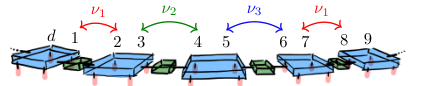
One possible architecture for universal computation on qubits consists in a closed linear array of quansistors coupled through resonators. Each quansistor represents a pair of qubits, and every qubit is represented exactly once (see Fig. 16). Additional qubit-splitting frequencies may be added to prevent untimely higher-order, th-nearest-neighbor couplings. To cut down space and running time costs, a physical implementation of the array would likely be folded, and a resonator would couple every adjacent pair of quansistors, thus reducing considerably the need for qubit-shuffling operations. Fig. 17 schematically depicts a planar-grid computer. Each quansistor would be coupled to four identical leads (not shown in the figure) for initialization and readout.
VI Outlook
Error-correcting codes are a promising avenue to make quantum computation fault-tolerant. In our technology, quansistors are the support of the physical qubits, whose states and interactions are symmetry-protected, to some extent, against external influences. Once we identify the dominant errors affecting them, we can find -qubit states (typically ) that are invariant under those errors. These would be encoded logical qubits. (In the standard Hamming notation, we get a code of type using physical qubits, and having logical codewords Steane 1996.) Having physical universality at hand gives the freedom to encode qubits and operations yielding encoded universality. Because our technology is scalable ( quansistors making qubits), the encoding uses identical ‘processors’ instead of one.
Crucially, we must determine whether the dominant errors are constrained by the symmetry of the quansistors. We have already observed a significant robustness of the universal set against single-qubit and double-qubit - and -rotation errors. As a second source of decoherence, we considered the coupling to semi-infinite leads, and have omitted other factors such as the effect of a heat bath on the system, the types of errors that it would produce, and the extent to which it would destroy symmetry.
Throughout, we have used -rotation invariance as the prototype of a symmetry of flat classes, universal for quantum computation, and realistically implementable physically. Other flat classes would perform equally well at protecting information and operations, as long as leads (or any other immediate environment of the clusters) do not break the corresponding symmetry. Universal sets of gates originating from nondegenerate Hamiltonians are symmetry-specific, but should not be too difficult to find given the relative scarcity of non-universal sets and the completeness of flat classes. The possibilities of physical implementation, on the other hand, will strongly depend on the chosen symmetry and would have to be found on a case-by-case basis.
There might be additional value to using larger qubit clusters, i.e. -qubit quansistors realized as sites with symmetries, for . All observations from the previous point regarding protection, universality, and implementation, apply here as well. Larger clusters and symmetry classes would offer protection to -qubit operations. It could also allow the encoding of a logical qubit within a single -qubit quansistor. Encodings with (8 sites) can already correct some single-qubit errors, while some encodings with (32 sites) can correct any single-qubit error Nielsen and Chuang 2010.
There is provable surplus value to using higher alphabets (ququarts, specifically), instead of qubit pairs, in encrypted communications Bechmann-Pasquinucci and Tittel 2000. Since -circulant 4-level quansistors are universal in , i.e. universal for single-ququart operations, and have the ability to dynamically decouple from the leads, a quansistor-with-leads could be a versatile memory unit for ququarts, and become an essential component of quantum-secure communications. Generalizations to -level quansistors (qudits), with , is also conceivable, as argued in the previous point. Error-correcting codes, notably, have been developed for qudits, that use Weyl matrices (or equivalently the version of our matrices and ) Gottesman 1999; Gottesman et al. 2001. Note, however, that the diagram of transition amplitudes of the general qudit ( in graph theory terminology) is non-planar for Rosen 2002, in contrast to the essentially planar diagram of the 4-level system, Fig. 8. A gauge potential implementation of -rotation invariant qudits, in the spirit of Sections III.5 and III.6, might then be essentially three-dimensional.
For the purpose of reconstructing the final state of an -qubit system, a symmetry based on Pauli tensors of dimension is better suited than -rotation invariance (based on Weyl matrices) as it allows for the maximal number () of mutually unbiased bases, and complete state characterization via state tomography Bandyopadhyay et al. 2001; Lawrence et al. 2001. By contrast, the 4-level quansistor () based on -rotation invariance has only three unbiased bases: , , , the respective eigenbases of . As for reconstructing the final state of an -qupit system (where is an odd prime), the Weyl-based scheme of dimension allows for the maximal number () of mutually unbiased bases, and complete state characterization via quantum tomography Bandyopadhyay et al. 2001; Durt et al. 2010. This could be of value for encrypted communication using a higher (prime) alphabet (see previous point), and could be based on -site quansistors with -rotation invariance.
To perform inter-quansistor interactions, we have used the simplest possible scenario involving a single qubit from each quansistor. It would be worth investigating whether a combined use of resonators and symmetry could make possible the implementation of robust 3- and 4-qubit gates, or even interactions soliciting three quansistors or more. However, this is beyond the scope of this work.
VII Conclusion
In this work, we have put forward a blueprint for scalable universal quantum computation based on 2-qubit clusters (quansistors) protected by symmetry (-rotation invariance). We find a significant robustness of the proposed universal set against single-qubit and double-qubit - and -rotation errors. Embedding in the environment, initialization and readout are achieved by tunnel-coupling each quansistor to four identical semi-infinite leads. We show that quansistors can be dynamically decoupled from the leads by tuning their internal parameters, giving them the versatility required to act as controllable quantum memory units. With this dynamical decoupling, universal 2-qubit logical operations within quansistors are also symmetry-protected against unbiased noise in their parameters. Two-quansistor entangling operations are achieved by resonator-coupling their qubit-splitting frequencies to effectively carry out the gate, with one qubit coming from each quansistor. We have also identified a variety of platforms that could implement -rotation invariance.
The complete tunability of -circulant quansistors can be exploited to build highly expressive and trainable parameterized quantum circuits, to be used as the noisy intermediate-scale quantum (NISQ) component of a quantum-classical hybrid machine learning model Benedetti et al. 2019; Sim et al. 2019; Holmes et al. 2022. These ideas will be explored in detail in a future publication.
VIII Acknowledgements
This work was supported in part by the Natural Science and Engineering Research Council of Canada and by the Fonds de Recherche Nature et Technologies du Québec via the INTRIQ strategic cluster grant. C.B. thanks the Department of National Defence of Canada for financial support to facilitate the completion of his PhD.
IX Appendices
Appendix A Mathematical framework
This section describes some mathematical aspects of -rotation invariance. Although this paper has focused on a four-level system, many of the results are easily generalized. Here we consider the more general case of an -level system. For multiple reasons it may be desirable to have full control over the eigenenergies of the system. In what follows we consider what we propose to call flat classes of Hamiltonians: classes of Hermitian matrices with a common eigenbasis, and real eigenenergies in one-to-one linear correspondence with the values of the parameters, that is with . (The term flat refers to vanishing Berry curvature in -space.) A class of Hamiltonians is flat in this sense if and only if it can be represented as a sum of Hermitian matrices,
| (98) |
and the matrix of all eigenvalues of the ’s is nonsingular, . (The key observation is the action of the diagonalizing unitary: .) Flat classes therefore coincide with -dimensional commutative algebras of Hermitian matrices, the nonsingularity of being equivalent to the linear independence of the ’s. Because each flat class is diagonalized by a common unitary (unique up to permutations), the set of all flat classes that correspond to the same is in one-to-one correspondence with unitaries modulo permutations. (In this paper, we do not consider non-unitarily diagonalizable matrices, like non-Hermitian -symmetric Hamiltonians, for instance.) The exponentials of a flat class also share the common eigenbasis of the class, and their eigenenergies are in (nonlinear) one-to-one correspondance with the values of the parameters . There seems to be an interesting connection between flat classes, on the one hand, and commuting bases of unitary matrices Bandyopadhyay et al. 2001 and stabilizers of quantum error-correcting codes Gottesman 1999, on the other.
For the purpose of quantum computation a single flat class is clearly not enough because it is commutative. The -circulant matrices defined in (6) are of the form (98), and constitute a flat class for each . Independent control over the energy levels is a prime motivation for using -rotation invariance, but we stress again that this choice of symmetry is far from unique. Starting from any nonsingular matrix , defining the functions , and applying any unitary to the matrix class will produce a commutative family of (Hermitian) Hamiltonian matrices with eigenstates independent of , and linearly controlled eigenenergies , i.e. a flat class. If symmetries other than -rotation invariance were preferred for practical reasons, one would replace the diagonalizing unitaries and , defined in Eqs. (9),(10), with the appropriate operations.
It is instructive to recast -rotations in terms of Sylvester’s clock-and-shift matrices (also called Weyl’s matrices or generalized Pauli matrices)
| (99) |
with . For we have the identity . The matrices constitute a non-Hermitian trace-orthogonal basis for , and in fact the same is true of their obvious -dimensional generalization, with , which span and are orthogonal under the Hilbert-Schmidt inner product. If , they reduce (up to a factor) to the Pauli matrices. The matrices and are central to Weyl’s formulation of periodic finite-dimensional quantum mechanics where they respectively correspond to finite position and momentum shifts:
| (100) | ||||
where of course and are position and momentum eigenstates, respectively. Thus -rotation invariance is a symmetry in quantum (or optical) phase space, and is not found in other, internal-space generalizations of Pauli matrices like Pauli tensor products or Gell-Mann matrices.
In any dimension , the eigenbases of , and are mutually unbiased: a measurement in one (orthonormal) basis provides no information about measurements in another (orthonormal) basis because for any . In particular when , the flat classes of , (the matrix in the main text), and (the matrix in the main text) have mutually unbiased eigenbases , and respectively. (See (15) and (21).)
Appendix B Effective core Hamiltonian
Consider an -level core tunnel-coupled to identical semi-infinite leads:
| (101) | ||||
For the time being, the matrix is not required to be Hermitian, and the couplings need not be equal, but could be chosen real positive with no loss of generality since the Hamiltonian is invariant under , . We let them be complex anyways. Let us restrict the system’s dynamics to the single-particle sector of Hilbert space. For illustration purposes, our examples below will use a core with levels, but all the results go over to general . The one-particle Hamiltonian matrix with is
| (102) |
which we write as
| (103) |
in obvious notation. The corresponding Green’s function is
| (104) | ||||
where is the identity on the single-lead space. The top-left block of the Green’s function, , can be obtained using the blockwise inversion formula
| (105) |
We obtain
| (106) | ||||
Noticing that
| (107) |
being the Green function of a single lead, we obtain from (106)
| (108) |
A straightforward calculation yields
| (109) |
where is the surface Green’s function of a single lead :
| (110) |
The analogous version of (109) for general is now obvious. Remarkably, if is -circulant and for all , the effective Hamiltonian is also -circulant:
| (111) |
In particular, when is Hermitian we obtain expression (59) in the main text. Again, the fact that is unaffected by the presence of phase factors, dynamical or stochastic, in the core-to-lead couplings is a consequence of (101) being invariant under , .
Appendix C Analytical solution: Two cores connected by finite leads
We analytically solve the Schrödinger equation of two -circulant -level cores (with the same , but possibly different core Hamiltonians and ) connected face-to-face by identical leads of sites. The Hamiltonian is
| (112) | ||||
where and . Leads have hopping energies all equal, and set to unity (thus setting the scale for all energies). Eigenvalues of the unitary symmetry (-rotation) correspond to superselection sectors. Without loss of generality, energy eigenstates may be chosen to have support in exactly one sector . If are -circulant with and , the change of basis Eqs. (9),(10)
| (113) |
decouples the system into identical modes, each in the form of two dots of self-energies connected by a finite lead of sites. The single-particle Hamiltonian for one of these modes is
| (114) |
Let be a single-particle eigenstate in sector , where is the state with a single particle in the th site. The Schrödinger equation yields the relations
| (115) | |||||
| (116) | |||||
| (117) | |||||
| (118) | |||||
| (119) |
where we have assumed that , and defined and . The bulk equation (116) is translation-invariant with general solution
| (120) |
The boundary conditions (115),(117) give the ratio
| (121) |
and the eigenenergies, , in implicit form
| (122) |
In terms of Chebyshev polynomials of the second kind
| (123) |
and recalling the recursion relation
| (124) |
we find
| (125) |
as in Eq.(72) of the main text. In the simplest case where and (identical dots, identical couplings), we have
| (126) |
The system’s eigenvalues coincide with the solutions of the above equation. Notice that for small the LHS is when is not in the vicinity of the singularities . This is illustrated in Fig. 11 of the main text for even (), and in Fig. 18 for odd (). In this symmetric case for which , all eigenstates are either symmetric or antisymmetric. This is seen from (121), which becomes , implying
| (127) |
Substituting in (120) gives .We must consider two cases: when is outside the energy band of the leads, and when it is within this energy band.
C.1 Bound states ( outside the band)
When is outside the energy band of the leads, we have if , and if , where is a real parameter. Then
| (128) |
with , where is a normalization factor, and where the eigenenergies satisfy the constraint
| (129) |
Alternatively, we can write the solution as
| (130) |
A generic feature of these bound states is their large amplitude at the dots. Because there are at least states from the continuous spectrum (see next section), there are at most two bound states. The bound states for and are displayed in Fig.12 a,b of the main text. The bound states for are plotted in Fig. 19 a,b.
In the limit , the constraint is equivalent to
| (131) |
yielding or . The resulting expressions for and describe bound states localized at either dot and decaying exponentially with distance over the characteristic length . Moreover, the constraint equations for are equivalent to the fixed-point relations and , respectively. These relations can be obtained as normalizability conditions on the eigenstates of a dot connected to a semi-infinite lead, by solving the corresponding Schrödinger equation. Alternatively, the Green’s function treatment of the core with semi-infinite leads, Appendix B, gives the same fixed-point relations as effective self-energies of the core once the leads are traced out. The bound state condition on for amounts to
| (132) |
or equivalently
| (133) |
with , in agreement with (65) from the main text. For , the condition on gives instead
| (134) |
with . Similar relations hold for the bound state condition on .
C.2 Scattering states ( within the band)
When , is real and we find
| (135) |
where is a normalization factor. For any finite , there are scattering states from the (perturbed) continuous spectrum of the lead. A generic feature of these states is their small amplitude at the quantum dots. Additionally, there can be two scattering hybridized states. A generic feature of these states is their relatively large amplitude on the dots. The hybridized states for and are displayed in Fig. 13 a,b. States from the (perturbed) continuous spectrum are displayed in Figs. 12 c,d, and 13 c,d. The hybridized states for and are displayed in Fig. 19 c,d.
References
- Nielsen and Chuang (2010) M. Nielsen and I. Chuang, Quantum Computation and Quantum Information (Cambridge University Press, Cambridge, 2010) 10th Anniversary Edition.
- Altman et al. (2021) E. Altman, K. R. Brown, G. Carleo, L. D. Carr, E. Demler, C. Chin, B. DeMarco, S. E. Economou, M. A. Eriksson, K.-M. C. Fu, M. Greiner, K. R. Hazzard, R. G. Hulet, A. J. Kollár, B. L. Lev, M. D. Lukin, R. Ma, X. Mi, S. Misra, C. Monroe, K. Murch, Z. Nazario, K.-K. Ni, A. C. Potter, P. Roushan, M. Saffman, M. Schleier-Smith, I. Siddiqi, R. Simmonds, M. Singh, I. Spielman, K. Temme, D. S. Weiss, J. Vučković, V. Vuletić, J. Ye, and M. Zwierlein, PRX Quantum 2, 017003 (2021).
- Zeng et al. (2015) B. Zeng, X. Chen, D. Zhou, and X.-G. Wen, Quantum Information Meets Quantum Matter – From Quantum Entanglement to Topological Phase in Many-Body Systems (Springer, New York, 2015).
- Giovannetti et al. (2004) V. Giovannetti, S. Lloyd, and L. Maccone, Science (New York, N.Y.) 306, 1330 (2004).
- Reck et al. (1994) M. Reck, A. Zeilinger, H. J. Bernstein, and P. Bertani, Phys. Rev. Lett. 73, 58 (1994).
- DiVincenzo (1995) D. P. DiVincenzo, Phys. Rev. A 51, 1015 (1995).
- Barenco (1995) A. Barenco, Proceedings of the Royal Society of London. Series A: Mathematical and Physical Sciences 449, 679 (1995).
- Barenco et al. (1995) A. Barenco, C. Bennett, R. Cleve, D. DiVincenzo, N. Margolus, P. Shor, T. Sleator, J. Smolin, and H. Weinfurter, Physical Review A 52 (1995), 10.1103/PhysRevA.52.3457.
- Kitaev (1997) A. Y. Kitaev, Russian Mathematical Surveys 52, 1191 (1997).
- Deutsch et al. (1995) D. Deutsch, A. Barenco, and A. Ekert, Proc. Roy. Soc. of London 449 (1995), 10.1098/rspa.1995.0065.
- Lloyd (1995) S. Lloyd, Phys. Rev. Lett. 75, 346 (1995).
- Bacon et al. (2001) D. Bacon, J. Kempe, D. P. DiVincenzo, D. A. Lidar, and K. B. Whaley, “Encoded universality in physical implementations of a quantum computer,” (2001), arXiv:quant-ph/0102140 [quant-ph] .
- Kempe et al. (2001) J. Kempe, D. Bacon, D. P. DiVincenzo, and K. B. Whaley, “Encoded universality from a single physical interaction,” (2001), arXiv:quant-ph/0112013 [quant-ph] .
- Aharonov (2003) D. Aharonov, “A simple proof that toffoli and hadamard are quantum universal,” (2003), arXiv:quant-ph/0301040 [quant-ph] .
- Shor (1997) P. W. Shor, SIAM Journal on Computing 26, 1484–1509 (1997).
- Lloyd (1996)
S. Lloyd, Science 273, 1073 (1996), https://science.sciencemag.org/content/273/5278/
1073.full.pdf . - Raz (1999) R. Raz, in Proceedings of the Thirty-First Annual ACM Symposium on Theory of Computing, STOC ’99 (Association for Computing Machinery, New York, NY, USA, 1999) p. 358–367.
- Gavinsky et al. (2007) D. Gavinsky, J. Kempe, I. Kerenidis, R. Raz, and R. de Wolf, in Proceedings of the Thirty-Ninth Annual ACM Symposium on Theory of Computing, STOC ’07 (Association for Computing Machinery, New York, NY, USA, 2007) p. 516–525.
- Le Gall (2006) F. Le Gall, Theory of Computing Systems 45 (2006), 10.1007/s00224-007-9097-3.
- Gottesman (1997) D. Gottesman, “Stabilizer codes and quantum error correction,” (1997), Caltech Ph.D. thesis, arXiv:quant-ph/9705052 [quant-ph] .
- Valiant (2001) L. G. Valiant, in Proceedings of the Thirty-Third Annual ACM Symposium on Theory of Computing, STOC ’01 (Association for Computing Machinery, New York, NY, USA, 2001) p. 114–123.
- Terhal and DiVincenzo (2001) B. Terhal and D. DiVincenzo, Physical Review A 65 (2001), 10.1103/PhysRevA.65.032325.
- Knill (2001) E. Knill, “Fermionic linear optics and matchgates,” (2001), arXiv:quant-ph/0108033 [quant-ph] .
- Knill et al. (2001) E. Knill, R. Laflamme, and G. J. Milburn, Nature 409, 46 (2001).
- Bravyi and Kitaev (2000) S. Bravyi and A. Kitaev, Annals of Physics 298 (2000), 10.1006/aphy.2002.6254.
- Valiant (1979) L. Valiant, Theoretical Computer Science 8, 189 (1979).
- Loss and DiVincenzo (1998) D. Loss and D. P. DiVincenzo, Phys. Rev. A 57, 120 (1998).
- Zwanenburg et al. (2013) F. A. Zwanenburg, A. S. Dzurak, A. Morello, M. Y. Simmons, L. C. Hollenberg, G. Klimeck, S. Rogge, S. N. Coppersmith, and M. A. Eriksson, Reviews of modern physics 85, 961 (2013).
- Watson et al. (2018) T. Watson, S. Philips, E. Kawakami, D. Ward, P. Scarlino, M. Veldhorst, D. Savage, M. Lagally, M. Friesen, S. Coppersmith, et al., nature 555, 633 (2018).
- Li et al. (2018) H.-O. Li, G. Cao, G.-D. Yu, M. Xiao, G.-C. Guo, H.-W. Jiang, and G.-P. Guo, Physical Review Applied 9, 024015 (2018).
- Nakamura et al. (1999) Y. Nakamura, Y. A. Pashkin, and J. S. Tsai, nature 398, 786 (1999).
- Devoret and Schoelkopf (2013) M. H. Devoret and R. J. Schoelkopf, Science 339, 1169 (2013).
- O’Brien et al. (2003) J. L. O’Brien, G. J. Pryde, A. G. White, T. C. Ralph, and D. Branning, Nature 426, 264 (2003).
- Blatt and Wineland (2008) R. Blatt and D. Wineland, Nature 453, 1008 (2008).
- Yao et al. (2012) N. Y. Yao, L. Jiang, A. V. Gorshkov, P. C. Maurer, G. Giedke, J. I. Cirac, and M. D. Lukin, Nature communications 3, 1 (2012).
- Nayak et al. (2008) C. Nayak, S. H. Simon, A. Stern, M. Freedman, and S. D. Sarma, Reviews of Modern Physics 80, 1083 (2008).
- Kiktenko et al. (2015a) E. O. Kiktenko, A. K. Fedorov, O. V. Man’ko, and V. I. Man’ko, Phys. Rev. A 91, 042312 (2015a).
- Kiktenko et al. (2015b) E. Kiktenko, A. Fedorov, A. Strakhov, and V. Man’ko, Physics Letters A 379, 1409 (2015b).
- Yan et al. (2018) F. Yan, P. Krantz, Y. Sung, M. Kjaergaard, D. Campbell, J. Wang, T. Orlando, S. Gustavsson, and W. Oliver, Physical Review Applied 10 (2018), 10.1103/PhysRevApplied.10.054062.
- Gottesman (1998) D. Gottesman, Physical Review A 57, 127 (1998).
- Sanders et al. (2015) Y. R. Sanders, J. J. Wallman, and B. C. Sanders, New Journal of Physics 18, 012002 (2015).
- Shor (1995) P. W. Shor, Physical review A 52, R2493 (1995).
- Palma et al. (1996) G. M. Palma, K.-A. Suominen, and A. Ekert, Proceedings of the Royal Society of London. Series A: Mathematical, Physical and Engineering Sciences 452, 567 (1996).
- Ischi et al. (2005) B. Ischi, M. Hilke, and M. Dubé, Physical Review B 71, 195325 (2005).
- Martinis et al. (2003) J. M. Martinis, S. Nam, J. Aumentado, K. Lang, and C. Urbina, Physical Review B 67, 094510 (2003).
- Preskill (2018) J. Preskill, Quantum 2, 79 (2018).
- Aidelsburger et al. (2018) M. Aidelsburger, S. Nascimbene, and N. Goldman, Comptes Rendus Physique 19, 394 (2018), quantum simulation / Simulation quantique.
- Vitanov (2020) N. Vitanov, Scientific Reports 10 (2020), 10.1038/s41598-020-61766-w.
- Frahm et al. (2004) K. M. Frahm, R. Fleckinger, and D. L. Shepelyansky, The European Physical Journal D - Atomic, Molecular and Optical Physics 29, 139–155 (2004).
- Sleator and Weinfurter (1995) T. Sleator and H. Weinfurter, Phys. Rev. Lett. 74, 4087 (1995).
- Wallman and Emerson (2016) J. J. Wallman and J. Emerson, Phys. Rev. A 94, 052325 (2016).
- Ware et al. (2021) M. Ware, G. Ribeill, D. Ristè, C. A. Ryan, B. Johnson, and M. P. da Silva, Phys. Rev. A 103, 042604 (2021).
- Hashim et al. (2021) A. Hashim, R. K. Naik, A. Morvan, J.-L. Ville, B. Mitchell, J. M. Kreikebaum, M. Davis, E. Smith, C. Iancu, K. P. O’Brien, I. Hincks, J. J. Wallman, J. Emerson, and I. Siddiqi, Phys. Rev. X 11, 041039 (2021).
- Perez et al. (2021) D. R. Perez, P. Varosy, Z. Li, T. Roy, E. Kapit, and D. Schuster, (2021), arXiv:2110.11537 [quant-ph] .
- Peres (1984) A. Peres, Phys. Rev. A 30, 1610 (1984).
- Cucchietti et al. (2005) F. M. Cucchietti, J. P. Paz, and W. H. Zurek, Physical Review A 72 (2005), 10.1103/physreva.72.052113.
- Goussev et al. (2012) A. Goussev, R. A. Jalabert, H. M. Pastawski, and A. Wisniacki, Scholarpedia 7, 11687 (2012).
- Berry (1984) M. V. Berry, Proceedings of the Royal Society of London. Series A, Mathematical and Physical Sciences 392, 45 (1984).
- Simon (1983) B. Simon, Phys. Rev. Lett. 51, 2167 (1983).
- Sørensen et al. (2005) A. S. Sørensen, E. Demler, and M. D. Lukin, Phys. Rev. Lett. 94, 086803 (2005).
- Wilczek and Zee (1984) F. Wilczek and A. Zee, Phys. Rev. Lett. 52, 2111 (1984).
- Mead (1992) C. A. Mead, Rev. Mod. Phys. 64, 51 (1992).
- Xiao et al. (2010) D. Xiao, M.-C. Chang, and Q. Niu, Rev. Mod. Phys. 82, 1959 (2010).
- Grifoni and Hänggi (1998) M. Grifoni and P. Hänggi, Physics Reports 304, 229 (1998).
- Dunlap and Kenkre (1986) D. H. Dunlap and V. M. Kenkre, Phys. Rev. B 34, 3625 (1986).
- Castro Neto et al. (2007) A. Castro Neto, F. Guinea, N. Peres, K. Novoselov, and A. Geim, Review of Modern Physics 81 (2007), 10.1103/RevModPhys.81.109.
- Hafezi (2013) M. Hafezi, International Journal of Modern Physics B 28 (2013), 10.1142/S0217979214410021.
- Ozawa et al. (2019) T. Ozawa, H. M. Price, A. Amo, N. Goldman, M. Hafezi, L. Lu, M. C. Rechtsman, D. Schuster, J. Simon, O. Zilberberg, and I. Carusotto, Rev. Mod. Phys. 91, 015006 (2019).
- Anderson et al. (2011) B. Anderson, G. Juzeliūnas, I. Spielman, and V. Galitski, Physical Review Letters 108 (2011), 10.1103/PhysRevLett.108.235301.
- Struck et al. (2012) J. Struck, C. Ölschläger, M. Weinberg, P. Hauke, J. Simonet, A. Eckardt, M. Lewenstein, K. Sengstock, and P. Windpassinger, Phys. Rev. Lett. 108, 225304 (2012).
- Hauke et al. (2012) P. Hauke, O. Tieleman, A. Celi, C. Ölschläger, J. Simonet, J. Struck, M. Weinberg, P. Windpassinger, K. Sengstock, M. Lewenstein, and A. Eckardt, Phys. Rev. Lett. 109, 145301 (2012).
- Aidelsburger et al. (2013) M. Aidelsburger, M. Atala, M. Lohse, J. T. Barreiro, B. Paredes, and I. Bloch, Phys. Rev. Lett. 111, 185301 (2013).
- Galitski and Spielman (2013) V. Galitski and I. Spielman, Nature 494, 49 (2013).
- Galitski et al. (2019) V. Galitski, G. Juzeliūnas, and I. B. Spielman, Physics Today 72, 38 (2019), arXiv:1901.03705 [cond-mat.quant-gas] .
- Bermudez et al. (2011) A. Bermudez, T. Schaetz, and D. Porras, Phys. Rev. Lett. 107, 150501 (2011).
- Bermudez et al. (2012) A. Bermudez, T. Schaetz, and D. Porras, New Journal of Physics 14, 053049 (2012).
- Aharony et al. (2012) A. Aharony, S. Gurvitz, Y. Tokura, O. Entin-Wohlman, and S. Dattagupta, Physica Scripta T151, 014018 (2012).
- Nilsson et al. (2006) H. Nilsson, C. Thelander, L. Fröberg, J. Wagner, and L. Samuelson, Applied Physics Letters 89, 163101 (2006).
- Aharon et al. (2016) E. Aharon, R. Pozner, E. Lifshitz, and U. Peskin, Journal of Applied Physics 120, 244301 (2016).
- Heshami et al. (2015) K. Heshami, D. England, P. Humphreys, P. Bustard, V. Acosta, J. Nunn, and B. Sussman, Journal of Modern Optics 63 (2015), 10.1080/09500340.2016.1148212.
- Saglamyurek et al. (2018) E. Saglamyurek, T. Hrushevskyi, A. Rastogi, K. Heshami, and L. LeBlanc, Nature Photonics 12 (2018), 10.1038/s41566-018-0279-0.
- Koong et al. (2020) Z.-X. Koong, G. Ballesteros-Garcia, R. Proux, D. Dalacu, P. J. Poole, and B. D. Gerardot, Phys. Rev. Applied 14, 034011 (2020).
- Blais et al. (2020) A. Blais, A. L. Grimsmo, S. M. Girvin, and A. Wallraff, “Circuit quantum electrodynamics,” (2020), arXiv:2005.12667 [quant-ph] .
- Steane (1996) A. Steane, Proceedings of the Royal Society A: Mathematical, Physical and Engineering Sciences 452 (1996), 10.1098/rspa.1996.0136.
- Bechmann-Pasquinucci and Tittel (2000) H. Bechmann-Pasquinucci and W. Tittel, Phys. Rev. A 61, 062308 (2000).
- Gottesman (1999) D. Gottesman, Chaos Solitons Fractals 10, 1749 (1999), arXiv:quant-ph/9802007 .
- Gottesman et al. (2001) D. Gottesman, A. Kitaev, and J. Preskill, Phys. Rev. A 64, 012310 (2001).
- Rosen (2002) K. H. Rosen, Discrete Mathematics and Its Applications, 5th ed. (McGraw-Hill Higher Education, 2002).
- Bandyopadhyay et al. (2001) S. Bandyopadhyay, P. Boykin, V. Roychowdhury, and F. Vatan, Algorithmica (New York) 34 (2001).
- Lawrence et al. (2001) J. Lawrence, C. Brukner, and A. Zeilinger, Physical Review A 65 (2001), 10.1103/PhysRevA.65.032320.
- Durt et al. (2010) T. Durt, B.-G. Englert, I. Bengtsson, and K. Życzkowski, International Journal of Quantum Information 08, 535 (2010), https://doi.org/10.1142/S0219749910006502 .
- Benedetti et al. (2019) M. Benedetti, E. Lloyd, S. Sack, and M. Fiorentini, Quantum Science and Technology 4, 043001 (2019).
- Sim et al. (2019) S. Sim, P. Johnson, and A. Aspuru-Guzik, Advanced Quantum Technologies 2 (2019), 10.1002/qute.201900070.
- Holmes et al. (2022) Z. Holmes, K. Sharma, M. Cerezo, and P. J. Coles, PRX Quantum 3, 010313 (2022).