跳到论文正文
W Papers独立论文阅读器 arXiv:2106.00581 论文正文 计算阅读时间 · 0%
引用这篇论文根据当前论文元数据生成,正式投稿前建议核对。


License: CC BY 4.0
arXiv:2106.00581v2 [q-fin.MF] 14 Jun 2021

NN-player and mean-field games in Itô-diffusion markets with competitive or homophilous interaction

Ruimeng Hu Thanks: Department of Mathematics and Department of Statistics & Applied Probability, University of California, Santa Barbara, CA 93106-3080, rhu@ucsb.edu.    Thaleia Zariphopoulou Thanks: Departments of Mathematics and IROM, The University of Texas at Austin, Austin, USA, and the Oxford-Man Institute, University of Oxford, Oxford, UK, zariphop@math.utexas.edu.
August 11, 2026
Abstract

In Itô-diffusion environments, we introduce and analyze NN-player and common-noise mean-field games in the context of optimal portfolio choice in a common market. The players invest in a finite horizon and also interact, driven either by competition or homophily. We study an incomplete market model in which the players have constant individual risk tolerance coefficients (CARA utilities). We also consider the general case of random individual risk tolerances and analyze the related games in a complete market setting. This randomness makes the problem substantially more complex as it leads to (NN or a continuum of) auxiliary “individual” Itô-diffusion markets. For all cases, we derive explicit or closed-form solutions for the equilibrium stochastic processes, the optimal state processes, and the values of the games.

1 Introduction

In Itô-diffusion environments, we introduce NN-player and common-noise mean-field games (MFGs) in the context of optimal portfolio choice in a common market. We build on the framework and notions of [12] (see, also, [11]) but allow for a more general market model (beyond the log-normal case) and, also, consider more complex risk preferences.

The paper consists of two parts. In the first part, we consider a common incomplete market and players with individual exponential utilities (CARA) who invest while interacting with each other, driven either by competition or homophily. We derive the equilibrium policies, which turn out to be state (wealth)-independent stochastic processes. Their forms depend on the market dynamics, the risk tolerance coefficients, and the underlying minimal martingale measure. We also derive the optimal wealth and the values of both the NN-player and the mean-field games, and discuss the competitive and homophilous cases.

In the second part, we assume that the common Itô-diffusion market is complete, but we generalize the model in the direction of risk preferences, allowing the risk tolerance coefficients to be random variables. For such preferences, we first analyze the single-player problem, which is interesting in its own right. Among others, we show that the randomness of the utility “distorts” the original market by inducing a “personalized” risk premium process. This effect is more pronounced in the NN-player game where the common market is now replaced by “personalized” markets whose stochastic risk premia depend on the individual risk tolerances. As a result, the tractability coming from the common market assumption is lost. In the MFG setting, these auxiliary individual markets are randomly selected (depending on the type vector) and aggregate to a common market with a modified risk premium process. We characterize the optimal policies, optimal wealth processes, and game values, building on the aforementioned single-player problem.

To our knowledge, NN-player games and MFGs in Itô-diffusion market settings have not been considered before except in preprint [6]. Therein, the authors used the same asset specialization framework and same CARA preferences as in [12] but allowed for Itô-diffusion price dynamics. They studied the problem using a forward-backward stochastic differential equation (FBSDE) approach. In our work, we have different model settings regarding both the measurability of the coefficients of the Itô-diffusion price processes and the individual risk tolerance inputs. We also solve the problems using a different approach, based on the analysis of portfolio optimization problems of exponential utilities in semi-martingale markets.

The theory of mean-field games was introduced by Lasry and Lions [13], who developed the fundamental elements of the mathematical theory and, independently, by Huang, Malhamé and Caines who considered a particular class [8]. Since then, the area has grown rapidly both in terms of theory and applications. Listing precise references is beyond the scope of this paper.

Our work contributes to NN-player games and MFG in Itô-diffusion settings for models with controlled processes whose dynamics depend linearly on the controls and are state-independent, and, furthermore, the controls appear in both the drift and the diffusion parts. Such models are predominant in asset pricing and in optimal portfolio and consumption choice. In the context of the general MFG theory, the models considered herein are restrictive. On the other hand, their structure allows us to produce explicit/closed-form solutions for Itô-diffusion environments.

The paper is organized as follows. In Section 2, we study the incomplete market case for both the NN-player game and the MFG, and for CARA utilities. In Section 3, we focus on the complete market case but allow for random risk tolerance coefficients. In analogy to Section 2, we analyze both the NN-player game and the MFG. We conclude in Section 4.

2 Incomplete Itô-diffusion common market and CARA utilities

We consider an incomplete Itô-diffusion market, in which we introduce an NN-player and a mean-field game for players who invest in a finite horizon while interacting among them, driven either by competition or homophily. We assume that the players (either at the finite or the continuum setting) have individual constant risk tolerance coefficients. For both the NN-player and the MFG, we derive in closed form the optimal policies, optimal controlled processes, and the game values. The analysis uses the underlying minimal martingale measure, related martingales, and their decomposition.

2.1 The NN-player game

Consider a probability space (Ω,ℱ,ℙ)(\Omega,\mathcal{F},\mathbb{P}) supporting two Brownian motions (Wt,WtY)t∈[0,T],(W_{t},W_{t}^{Y})_{t\in[0,T]}, T<∞,T<\infty, imperfectly correlated with the correlation coefficient ρ∈(−1,1)\rho\in\left(-1,1\right). We denote by (ℱt)t∈[0,T](\mathcal{F}_{t})_{t\in[0,T]} the natural filtration generated by both WW and WYW^{Y}, and by (𝒢t)t∈[0,T](\mathcal{G}_{t})_{t\in[0,T]} the one generated only by WYW^{Y}. We then let (μt)t∈[0,T](\mu_{t})_{t\in[0,T]} and (σt)t∈[0,t](\sigma_{t})_{t\in\left[0,t\right]} be 𝒢t\mathcal{G}_{t}-adapted processes, with 0<c≤σt≤C0<c\leq\sigma_{t}\leq C and |μt|≤C\left|\mu_{t}\right|\leq C, t∈[0,T]t\in\left[0,T\right], for some (possibly deterministic) constants cc and CC.

The financial market consists of a riskless bond (taken to be the numeraire and with zero interest rate) and a stock whose price process (St)t∈[0,T](S_{t})_{t\in\left[0,T\right]} satisfies

d​St=μt​St​d​t+σt​St​d​Wt,S0=s0∈ℝ+.\,dS_{t}=\mu_{t}S_{t}\,dt+\sigma_{t}S_{t}\,dW_{t},\quad S_{0}=s_{0}\in\mathbb{R}^{+}. (2.1)

In this market, NN players, indexed by i∈ℐ,i\in\mathcal{I}, ℐ={1,2,…,N}\mathcal{I}=\left\{1,2,\ldots,N\right\}, have a common investment horizon [0,T]\left[0,T\right] and trade between the two accounts. Each player, say player i,i, uses a self-financing strategy (πti)t∈[0,T](\pi_{t}^{i})_{t\in[0,T]}, representing (discounted by the numeraire) the amount invested in the stock. Then, her wealth (Xti)t∈[0,T](X_{t}^{i})_{t\in[0,T]} satisfies

d​Xti=πti​(μt​d​t+σt​d​Wt),X0i=xi∈ℝ,\,dX_{t}^{i}=\pi_{t}^{i}\left(\mu_{t}\,dt+\sigma_{t}\,dW_{t}\right),\quad\ \ X_{0}^{i}=x_{i}\in\mathbb{R}, (2.2)

with πi\pi^{i} being an admissible policy, belonging to

𝒜={π:self-financing, ​ℱ​-progressively measurable and ​Eℙ​[∫0Tσs2​πs2​𝑑s]<∞}.\mathcal{A}=\left\{\pi:\text{self-financing, }\mathcal{F}\text{-progressively measurable and }E_{\mathbb{P}}\left[\int_{0}^{T}\sigma_{s}^{2}\pi_{s}^{2}\,ds\right]<\infty\right\}. (2.3)

As in [12] (see also [1, 4, 9, 10, 11, 20]), players optimize their expected terminal utility but are, also, concerned with the performance of their peers. For an arbitrary but fixed policy (π1,…,πi−1,πi+1,…,πN)(\pi_{1},\ldots,\pi_{i-1},\pi_{i+1},\ldots,\pi_{N}), player ii, i∈ℐi\in\mathcal{I}, seeks to optimize

Vi(x1,…,xi,…,xN)=supπi∈𝒜Eℙ[−exp(−1δi(XTi−ciCT))|X01=x1,…,X0i=xi,…,X0N=xN],V^{i}\left(x_{1},\ldots,x_{i},\ldots,x_{N}\right)=\sup_{\pi^{i}\in\mathcal{A}}E_{\mathbb{P}}\left[\left.-\exp\left(-\frac{1}{\delta_{i}}\left(X_{T}^{i}-c_{i}C_{T}\right)\right)\right|X_{0}^{1}=x_{1},\ldots,X_{0}^{i}=x_{i},\ldots,X_{0}^{N}=x_{N}\right], (2.4)

where

CT:=1N​∑j=1NXTjC_{T}:=\frac{1}{N}\sum_{j=1}^{N}X_{T}^{j} (2.5)

averages all players’ terminal wealth, with XTjX_{T}^{j}, j=1,…,Nj=1,\ldots,N, given by (2.2).

The parameter δi>0\delta_{i}>0 is the individual (absolute) risk tolerance while the constant ci∈(−∞,1]c_{i}\in(-\infty,1] models the individual interaction weight towards the average wealth of all players. If ci>0c_{i}>0, the above criterion models competition while when ci<0c_{i}<0 it models homophilous interactions (see, for example, [14]). The optimization criterion (2.4) can be, then, viewed as a stochastic game among the NN players, where the notion of optimality is being considered in the context of a Nash equilibrium, stated below (see, for example, [2]).

Definition 2.1.

A strategy (πt∗)t∈[0,T]=(πt1,∗,…,πtN,∗)t∈[0,T]∈𝒜⊗N(\pi_{t}^{\ast})_{t\in\left[0,T\right]}=(\pi_{t}^{1,\ast},\ldots,\pi_{t}^{N,\ast})_{t\in[0,T]}\in\mathcal{A}^{\otimes N} is called a Nash equilibrium if, for each i∈ℐi\in\mathcal{I} and πi∈𝒜,\pi^{i}\in\mathcal{A},

Eℙ[−exp(−1δi(XTi,∗−ciCT∗))|X01=x1,…,X0i=xi,…,X0N=xN]≥Eℙ[−exp(−1δi(XTi−ciCTi,∗))|X01=x1,…,X0i=xi,…,X0N=xN]E_{\mathbb{P}}\left[\left.-\exp\left(-\frac{1}{\delta_{i}}\left(X_{T}^{i,\ast}-c_{i}C_{T}^{\ast}\right)\right)\right|X_{0}^{1}=x_{1},\ldots,X_{0}^{i}=x_{i},\ldots,X_{0}^{N}=x_{N}\right]\\ \geq E_{\mathbb{P}}\left[\left.-\exp\left(-\frac{1}{\delta_{i}}\left(X_{T}^{i}-c_{i}C_{T}^{i,\ast}\right)\right)\right|X_{0}^{1}=x_{1},\ldots,X_{0}^{i}=x_{i},\ldots,X_{0}^{N}=x_{N}\right] (2.6)

with

CT∗:=1N∑j=1NXTj,∗ and CTi,∗:=1N(∑j=1,j≠iNXTj,∗+XTi), C_{T}^{\ast}:=\frac{1}{N}\sum_{j=1}^{N}X_{T}^{j,\ast}\text{ \ \ and \ \ }C_{T}^{i,\ast}:=\frac{1}{N}\left(\sum_{j=1,j\neq i}^{N}X_{T}^{j,\ast}+X_{T}^{i}\right),\text{\ }

where XTj,∗X_{T}^{j,\ast}, j∈ℐj\in\mathcal{I}, solve (2.2) with πj,∗\pi^{j,\ast} being used.

In this incomplete market, we recall the associated minimal martingale measure ℚM​M\mathbb{Q}^{MM}, defined on ℱT,\mathcal{F}_{T}, with

d​ℚM​Md​ℙ=exp(−12∫0Tλs2ds−∫0TλsdWs),\frac{\,d\mathbb{Q}^{MM}}{\,d\mathbb{P}}=\exp\left(-\frac{1}{2}\int_{0}^{T}\lambda_{s}^{2}\,ds-\int_{0}^{T}\lambda_{s}\,dW_{s}\right), (2.7)

where λt:=μtσt\lambda_{t}:=\frac{\mu_{t}}{\sigma_{t}}, t∈[0,T]t\in[0,T], is the Sharpe ratio process (see, among others, [5]). By the assumptions on the model coefficients, we have that, for t∈[0,T]t\in\left[0,T\right], λt∈𝒢t\lambda_{t}\in\mathcal{G}_{t} and

|λt|≤K,\left|\lambda_{t}\right|\leq K, (2.8)

for some (possibly deterministic) constant KK. We also consider the processes (W~t)t∈[0,T](\widetilde{W}_{t})_{t\in\left[0,T\right]} and (W~tY)t∈[0,T](\widetilde{W}_{t}^{Y})_{t\in[0,T]} with W~t=Wt+∫0tλs​𝑑s\widetilde{W}_{t}=W_{t}+\int_{0}^{t}\lambda_{s}\,ds and W~tY=WtY+ρ​∫0tλs​𝑑s,\widetilde{W}_{t}^{Y}=W_{t}^{Y}+\rho\int_{0}^{t}\lambda_{s}\,ds, which are standard Brownian motions under ℚM​M\mathbb{Q}^{MM} with W~t∈ℱt\widetilde{W}_{t}\in\mathcal{F}_{t} and W~tY∈𝒢t.\widetilde{W}_{t}^{Y}\in\mathcal{G}_{t}.

Next, we introduce the ℚM​M\mathbb{Q}^{MM}-martingale (Mt)t∈[0,T](M_{t})_{t\in\left[0,T\right]},

Mt:=EℚM​M[e−12(1−ρ2)∫0Tλs2ds|𝒢t].M_{t}:=E_{\mathbb{Q}^{MM}}\left[\left.e^{-\frac{1}{2}(1-\rho^{2})\int_{0}^{T}\lambda_{s}^{2}\,ds}\right|\mathcal{G}_{t}\right]. (2.9)

From (2.8) and the martingale representation theorem, there exists a 𝒢t\mathcal{G}_{t}-adapted process ξ∈ℒ2​(ℙ)\xi\in\mathcal{L}^{2}\left(\mathbb{P}\right) such that

d​Mt=ξt​Mt​d​W~tY=ξt​Mt​(ρ​d​W~t+1−ρ2​d​Wt⟂),\,dM_{t}=\xi_{t}M_{t}\,d\widetilde{W}_{t}^{Y}=\xi_{t}M_{t}\left(\rho\,d\widetilde{W}_{t}+\sqrt{1-\rho^{2}}\,dW_{t}^{\perp}\right), (2.10)

where Wt⟂W_{t}^{\perp} is a standard Brownian motion independent of WtW_{t} appearing in the decomposition WtY=ρ​Wt+1−ρ2​Wt⟂W_{t}^{Y}=\rho W_{t}+\sqrt{1-\rho^{2}}W_{t}^{\perp}.

In the absence of interaction among the players (ci≡0,c_{i}\equiv 0, OPENi∈ℐ),i\in\mathcal{I}), the optimization problem (2.4) has been analyzed by various authors (see, among others, [17, 18]). We recall its solution which will be frequently used herein.

Lemma 2.2 (no interaction).

Consider the optimization problem

v(x)=supa∈𝒜Eℙ[−e−1δ​xT|x0=x],v(x)=\sup_{a\in\mathcal{A}}E_{\mathbb{P}}\left[\left.-e^{-\frac{1}{\delta}x_{T}}\right|x_{0}=x\right], (2.11)

with δ>0\delta>0 and (xt)t∈[0,T](x_{t})_{t\in\left[0,T\right]} solving

d​xt=at​(μt​d​t+σt​d​Wt),x0=x∈ℝ,a∈𝒜.\,dx_{t}=a_{t}\left(\mu_{t}\,dt+\sigma_{t}\,dW_{t}\right),\quad x_{0}=x\in\mathbb{R},\quad a\in\mathcal{A}. (2.12)

Then, the optimal policy (at∗)t∈[0,T]\left(a_{t}^{\ast}\right)_{t\in\left[0,T\right]} and the value function are given by

at∗=δ⁡(λtσt+ρ1−ρ2​ξtσt),a_{t}^{\ast}=\delta\left(\frac{\lambda_{t}}{\sigma_{t}}+\frac{\rho}{1-\rho^{2}}\frac{\xi_{t}}{\sigma_{t}}\right), (2.13)

and

v(x)=−e−1δ​xM011−ρ2=−e−1δ​x(EℚM​M[e−12(1−ρ2)∫0Tλs2ds])11−ρ2,v(x)=-e^{-\frac{1}{\delta}x}M_{0}^{\frac{1}{1-\rho^{2}}}=-e^{-\frac{1}{\delta}x}\left(E_{\mathbb{Q}^{MM}}\left[e^{-\frac{1}{2}(1-\rho^{2})\int_{0}^{T}\lambda_{s}^{2}\,ds}\right]\right)^{\frac{1}{1-\rho^{2}}}, (2.14)

with (ξt)t∈[0,T]\left(\xi_{t}\right)_{t\in\left[0,T\right]} as in (2.10).

Proof.

We only present the key steps, showing that the process (ut)t∈[0,T],\left(u_{t}\right)_{t\in\left[0,T\right]},

ut:=−e−1δ​xt(EℚM​M[e−12(1−ρ2)∫tTλs2ds|𝒢t])11−ρ2,u_{t}:=-e^{-\frac{1}{\delta}x_{t}}\left(E_{\mathbb{Q}^{MM}}\left[\left.e^{-\frac{1}{2}(1-\rho^{2})\int_{t}^{T}\lambda_{s}^{2}\,ds}\right|\mathcal{G}_{t}\right]\right)^{\frac{1}{1-\rho^{2}}},

with u0=v⁡(x),u_{0}=v(x), x∈ℝ,x\in\mathbb{R}, is a supermartingale for xtx_{t} solving (2.12) for arbitrary α∈𝒜\alpha\in\mathcal{A} and becomes a martingale for α∗\alpha^{\ast} as in (2.13). To this end, we write

ut=−e−xtδ​Mt11−ρ2​eNtwith ​Nt=12​∫0tλu2​𝑑u,u_{t}=-e^{-\frac{x_{t}}{\delta}}M_{t}^{\frac{1}{1-\rho^{2}}}e^{N_{t}}\quad\text{with \ \ }N_{t}=\frac{1}{2}\int_{0}^{t}\lambda_{u}^{2}\,du,

and observe that

d​ut\displaystyle\,du_{t} =−utδ​d​xt+12​δ2​ut​d​⟨x⟩t+ut​d​Nt+11−ρ2​utMt​d​Mt\displaystyle=-\frac{u_{t}}{\delta}\,dx_{t}+\frac{1}{2\delta^{2}}u_{t}\,d\langle x\rangle_{t}+u_{t}\,dN_{t}+\frac{1}{1-\rho^{2}}\frac{u_{t}}{M_{t}}\,dM_{t}\,
+12​(1−ρ2)​ρ21−ρ2​utMt2​d​⟨M⟩t−1δ⁡(1−ρ2)​utMt​d​⟨x,M⟩t\displaystyle\qquad+\frac{1}{2(1-\rho^{2})}\frac{\rho^{2}}{1-\rho^{2}}\frac{u_{t}}{M_{t}^{2}}\,d\langle M\rangle_{t}-\frac{1}{\delta(1-\rho^{2})}\frac{u_{t}}{M_{t}}\,d\langle x,M\rangle_{t}
=ut​(−1δ​at​μt+12​1δ2​at2​σt2+12​λt2+ρ1−ρ2​ξt​λt+ρ22​(1−ρ2)2​ξt2−ρδ⁡(1−ρ2)​at​σt​ξt)​d​t\displaystyle=u_{t}\left(-\frac{1}{\delta}a_{t}\mu_{t}+\frac{1}{2}\frac{1}{\delta^{2}}a_{t}^{2}\sigma_{t}^{2}+\frac{1}{2}\lambda_{t}^{2}+\frac{\rho}{1-\rho^{2}}\xi_{t}\lambda_{t}+\frac{\rho^{2}}{2(1-\rho^{2})^{2}}\xi_{t}^{2}-\frac{\rho}{\delta(1-\rho^{2})}a_{t}\sigma_{t}\xi_{t}\right)dt
+ut​(−1δ​at​σt​d​Wt+11−ρ2​ξt​d​WtY)\displaystyle\qquad+u_{t}\left(-\frac{1}{\delta}a_{t}\sigma_{t}\,dW_{t}+\frac{1}{1-\rho^{2}}\xi_{t}\,dW_{t}^{Y}\right)
=12​ut​(−1δ​σt​at+λt+ρ1−ρ2​ξt)2​d​t+ut​(−1δ​at​σt​d​Wt+11−ρ2​ξt​d​WtY).\displaystyle=\frac{1}{2}u_{t}\left(-\frac{1}{\delta}\sigma_{t}a_{t}+\lambda_{t}+\frac{\rho}{1-\rho^{2}}\xi_{t}\right)^{2}dt+u_{t}\left(-\frac{1}{\delta}a_{t}\sigma_{t}\,dW_{t}+\frac{1}{1-\rho^{2}}\xi_{t}\,dW_{t}^{Y}\right).

Because ut<0,u_{t}<0, the drift remains non-positive and vanishes for t∈[0,T]t\in\left[0,T\right] if and only if the policy

at∗=δ⁡(λtσt+ρ1−ρ2​ξtσt)a_{t}^{\ast}=\delta\left(\frac{\lambda_{t}}{\sigma_{t}}+\frac{\rho}{1-\rho^{2}}\frac{\xi_{t}}{\sigma_{t}}\right)

is being used. Furthermore, a∗∈𝒜,a^{\ast}\in\mathcal{A}, as it follows from the boundedness assumption on σ\sigma, inequality (2.8) and that ξ∈ℒ2​(ℙ).\xi\in\mathcal{L}^{2}\left(\mathbb{P}\right). The rest of the proof follows easily. ∎

Next, we present the first main result herein that yields the existence of a (wealth-independent) stochastic Nash equilibrium.

Proposition 2.3.

For δi>0\delta_{i}>0 and ci∈(−∞,1]c_{i}\in(-\infty,1], introduce the quantities

φN:=1N​∑i=1Nδi​ and ​ψN:=1N​∑i=1Nci,\varphi_{N}:=\frac{1}{N}\sum_{i=1}^{N}\delta_{i}\text{ \ \ \ \ and \ \ \ }\psi_{N}:=\frac{1}{N}\sum_{i=1}^{N}c_{i}, (2.15)

and

δ¯i:=δi+φN1−ψN​ci.\bar{\delta}_{i}:=\delta_{i}+\frac{\varphi_{N}}{1-\psi_{N}}c_{i}. (2.16)

The following assertions hold:

  1. 1.

    If ψN<1\psi_{N}<1, there exists a wealth-independent Nash equilibrium, (πt∗)t∈[0,T]=(πt1,∗,…,πti,∗,…,πtN,∗)t∈[0,T]\left(\pi_{t}^{\ast}\right)_{t\in\left[0,T\right]}=\left(\pi_{t}^{1,\ast},\ldots,\pi_{t}^{i,\ast},\ldots,\pi_{t}^{N,\ast}\right)_{t\in\left[0,T\right]}, where πti,∗\pi_{t}^{i,\ast}, i∈ℐi\in\mathcal{I}, is given by the 𝒢t\mathcal{G}_{t}-adapted process

    πti,∗=δ¯i​(λtσt+ρ1−ρ2​ξtσt),\pi_{t}^{i,\ast}=\bar{\delta}_{i}\left(\frac{\lambda_{t}}{\sigma_{t}}+\frac{\rho}{1-\rho^{2}}\frac{\xi_{t}}{\sigma_{t}}\right), (2.17)

    with (ξt)t∈[0,T](\xi_{t})_{t\in\left[0,T\right]} as in (2.10). The associated optimal wealth process (Xti,∗)t∈[0,T]\left(X_{t}^{i,\ast}\right)_{t\in\left[0,T\right]} is

    Xti,∗=xi+δ¯i​∫0t(λu+ρ1−ρ2​ξu)​(λu​𝑑u+d​Wu)X_{t}^{i,\ast}=x_{i}+\bar{\delta}_{i}\int_{0}^{t}\left(\lambda_{u}+\frac{\rho}{1-\rho^{2}}\xi_{u}\right)\left(\lambda_{u}\,du+\,dW_{u}\right) (2.18)

    and the game value for player ii, i∈ℐi\in\mathcal{I}, is given by

    Vi​(x1,x2,…,xN)\displaystyle V^{i}\left(x_{1},x_{2},\ldots,x_{N}\right) =−exp⁡(−1δi​(xi−ci​x¯))​M011−ρ2\displaystyle=-\exp\left(-\frac{1}{{\delta}_{i}}\left(x_{i}-c_{i}\bar{x}\right)\right)M_{0}^{\frac{1}{1-\rho^{2}}}
    =−exp(−1δi(xi−cix¯))(EℚM​M[e−12(1−ρ2)∫0Tλs2ds])11−ρ2,\displaystyle=-\exp\left(-\frac{1}{{\delta}_{i}}\left(x_{i}-c_{i}\bar{x}\right)\right)\left(E_{\mathbb{Q}^{MM}}\left[e^{-\frac{1}{2}(1-\rho^{2})\int_{0}^{T}\lambda_{s}^{2}\,ds}\right]\right)^{\frac{1}{1-\rho^{2}}}, (2.19)

    with x¯=1N​∑i=1Nxi\bar{x}=\frac{1}{N}\sum_{i=1}^{N}x_{i}.

  2. 2.

    If ψN=1\psi_{N}=1, then it must be that ci≡1c_{i}\equiv 1, for all i∈ℐi\in\mathcal{I}, and there is no such wealth-independent Nash equilibrium.

Proof.

We first solve the individual optimization problem (2.4) for player i∈ℐi\in\mathcal{I}, taking the (arbitrary) strategies (π1,…,πi−1,πi+1,…,πN)(\pi^{1},\ldots,\pi^{i-1},\pi^{i+1},\ldots,\pi^{N}) of all other players as given. This problem can be alternatively written as

vi(x~i)=supπ~i∈𝒜𝔼ℙ[−exp(−1δix~Ti)|x~0i=x~i],v^{i}\left(\tilde{x}_{i}\right)=\sup_{\widetilde{\pi}^{i}\in\mathcal{A}}\mathbb{E}_{\mathbb{P}}\left[\left.-\exp\left(-\frac{1}{\delta_{i}}\tilde{x}_{T}^{i}\right)\right|\tilde{x}_{0}^{i}=\tilde{x}_{i}\right], (2.20)

where x~ti:=Xti−ciN​∑j=1NXtj\tilde{x}_{t}^{i}:=X_{t}^{i}-\frac{c_{i}}{N}\sum_{j=1}^{N}X_{t}^{j}, t∈[0,T],t\in\left[0,T\right], solves

d​x~ti=π~ti​(μt​d​t+σt​d​Wt)​ and ​x~0i=x~i:=xi−ci​x¯.\,d\tilde{x}_{t}^{i}=\widetilde{\pi}_{t}^{i}\left(\mu_{t}\,dt+\sigma_{t}\,dW_{t}\right)\text{ \ \ \ and \ \ }\tilde{x}_{0}^{i}=\tilde{x}_{i}:=x_{i}-c_{i}\bar{x}.

From Lemma 2.2, we deduce that its optimal policy is given by

π~ti,∗=δi​(λtσt+ρ1−ρ2​ξtσt),\widetilde{\pi}_{t}^{i,\ast}=\delta_{i}\left(\frac{\lambda_{t}}{\sigma_{t}}+\frac{\rho}{1-\rho^{2}}\frac{\xi_{t}}{\sigma_{t}}\right),

and thus the optimal policy of (2.4) can be written as

πti,∗=δi​(λtσt+ρ1−ρ2​ξtσt)+ciN​(∑j≠iπtj+πti,∗).\pi_{t}^{i,\ast}=\delta_{i}\left(\frac{\lambda_{t}}{\sigma_{t}}+\frac{\rho}{1-\rho^{2}}\frac{\xi_{t}}{\sigma_{t}}\right)+\frac{c_{i}}{N}\left(\sum_{j\neq i}\pi_{t}^{j}+\pi_{t}^{i,\ast}\right). (2.21)

Symmetrically, all players j∈ℐj\in\mathcal{I} follow an analogous to (2.21) strategy. Averaging over j∈ℐj\in\mathcal{I} yields

1N​∑i=1Nπti,∗=ψN​1N​∑i=1Nπti,∗+φN​(λtσt+ρ1−ρ2​ξtσt),\frac{1}{N}\sum_{i=1}^{N}\pi_{t}^{i,\ast}=\psi_{N}\frac{1}{N}\sum_{i=1}^{N}\pi_{t}^{i,\ast}+\varphi_{N}\left(\frac{\lambda_{t}}{\sigma_{t}}+\frac{\rho}{1-\rho^{2}}\frac{\xi_{t}}{\sigma_{t}}\right),

with ψN\psi_{N} and φN\varphi_{N} as in (2.15). If ψN<1\psi_{N}<1, the above equation gives

1N​∑i=1Nπti,∗=φN1−ψN​(λtσt+ρ1−ρ2​ξtσt),\frac{1}{N}\sum_{i=1}^{N}\pi_{t}^{i,\ast}=\frac{\varphi_{N}}{1-\psi_{N}}\left(\frac{\lambda_{t}}{\sigma_{t}}+\frac{\rho}{1-\rho^{2}}\frac{\xi_{t}}{\sigma_{t}}\right),

and we obtain (2.17). The rest of the proof follows easily. ∎

We have stated the above result assuming that we start at t=0t=0. This is without loss of generality, as all arguments may be modified accordingly. For completeness, we present in the sequel the time-dependent case, in the context of a Markovian market.

Remark 2.4.

As discussed in [12, Remark 2.5], problem (2.4) may be alternatively and equivalently represented as

Vi(x1,…,xN)=supπi∈𝒜Eℙ[−exp(−1δi′(XTi−ci′CT−i))|X01=x1,…,X0i=xi,…,X0N=xN],V^{i}(x_{1},\ldots,x_{N})=\sup_{\pi^{i}\in\mathcal{A}}E_{\mathbb{P}}\left[\left.-\exp\left(-\frac{1}{\delta_{i}^{\prime}}\left(X_{T}^{i}-c_{i}^{\prime}C_{T}^{-i}\right)\right)\right|X_{0}^{1}=x_{1},\ldots,X_{0}^{i}=x_{i},\ldots,X_{0}^{N}=x_{N}\right],

with CT−i:=1N−1​∑j=1,j≠iNXTjC_{T}^{-i}:=\frac{1}{N-1}\sum_{j=1,j\neq i}^{N}X_{T}^{j}, and δi=δi′1+1N−1​ci′\delta_{i}=\frac{\delta_{i}^{\prime}}{1+\frac{1}{N-1}c_{i}^{\prime}} and ci=ci′N−1N+ci′Nc_{i}=\frac{c_{i}^{\prime}}{\frac{N-1}{N}+\frac{c_{i}^{\prime}}{N}}.

Remark 2.5.

Instead of working with the minimal martingale measure in the incomplete Itô-diffusion market herein, one may employ the minimal entropy measure, ℚM​E\mathbb{Q}^{ME}, given by

d​ℚM​Ed​ℙ=exp(−12∫0T(λs2+χs2)ds−∫0TλsdWs−∫0TχsdWs⟂),\frac{d\mathbb{Q}^{ME}}{d\mathbb{P}}=\exp\left(-\frac{1}{2}\int_{0}^{T}\left(\lambda_{s}^{2}+\chi_{s}^{2}\right)\,ds-\int_{0}^{T}\lambda_{s}\,dW_{s}-\int_{0}^{T}\chi_{s}\,dW_{s}^{\perp}\ \right), (2.22)

where χt=−Zt⟂\chi_{t}=-Z_{t}^{\perp} and (yt,Zt,Zt⟂)t∈[0,T]\left(y_{t},Z_{t},Z_{t}^{\perp}\right)_{t\in\left[0,T\right]} solves the backward stochastic differential equation (BSDE)

−d​yt=(−12​λt2+12​(Zt⟂)2−λt​Zt)​d​t−(Zt​d​Wt+Zt⟂​d​Wt⟂)​ and ​yT=0.-dy_{t}=\left(-\frac{1}{2}\lambda_{t}^{2}+\frac{1}{2}(Z_{t}^{\perp})^{2}-\lambda_{t}Z_{t}\right)dt-\left(Z_{t}\,dW_{t}+Z_{t}^{\perp}\,dW_{t}^{\perp}\right)\text{ \ and \ \ }y_{T}=0. (2.23)

The measures ℚM​E\mathbb{Q}^{ME} and ℚM​M\mathbb{Q}^{MM} are related through the relative entropy ℋ\mathcal{H} in that −ℋ⁡(ℚM​E|ℙ)=11−ρ2​ln⁡M0-\mathcal{H}(\mathbb{Q}^{ME}|\mathbb{P})=\frac{1}{1-\rho^{2}}\ln M_{0} (cf. [17]). We choose to work with ℚM​M\mathbb{Q}^{MM} for ease of the presentation.

From Lemma 2.2, we see that the Nash equilibrium process,

πti,∗=δ¯i​(λtσt+ρ1−ρ2​ξtσt),\pi_{t}^{i,\ast}=\bar{\delta}_{i}\left(\frac{\lambda_{t}}{\sigma_{t}}+\frac{\rho}{1-\rho^{2}}\frac{\xi_{t}}{\sigma_{t}}\right),

resembles the optimal policy of an individual player of the classical optimal investment problem with exponential utility and modified risk tolerance, δ¯i.\bar{\delta}_{i}. The latter deviates from δi\delta_{i} by

δ¯i−δi=φN1−ψN​ci.\bar{\delta}_{i}-\delta_{i}=\frac{\varphi_{N}}{1-\psi_{N}}c_{i}.

In the competitive case, ci>0c_{i}>0, δ¯i>δi\bar{\delta}_{i}>\delta_{i} and their difference increases with cic_{i}, φN\varphi_{N} and ψN\psi_{N}. At times tt such that λtσt+ρ1−ρ2​ξtσt>0\frac{\lambda_{t}}{\sigma_{t}}+\frac{\rho}{1-\rho^{2}}\frac{\xi_{t}}{\sigma_{t}}>0 (resp. λtσt+ρ1−ρ2​ξtσt\frac{\lambda_{t}}{\sigma_{t}}+\frac{\rho}{1-\rho^{2}}\frac{\xi_{t}}{\sigma_{t}} OPEN<0)<0), the competition concerns make the player invest more (resp. less) in the risky asset than without such concerns.

In the homophilous case, ci<0c_{i}<0, we have that δ¯i<δi\bar{\delta}_{i}<\delta_{i}. Furthermore, direct computations show that their difference decreases with δi\delta_{i} and each cjc_{j}, j≠ij\neq i, while it increases with cic_{i}. In other words,

∂δj(δ¯i−δi)<0, ∀j∈ℐ, ∂cj(δ¯i−δi)<0, ∀j∈ℐ∖{i}, and ∂ci(δ¯i−δi)>0.\partial_{\delta_{j}}\left(\bar{\delta}_{i}-\delta_{i}\right)<0,\text{ }\forall j\in\mathcal{I},\text{ \ \ }\partial_{c_{j}}\left(\bar{\delta}_{i}-\delta_{i}\right)<0,\text{ }\forall j\in\mathcal{I\smallsetminus}\left\{i\right\}\text{, \ \ and \ \ }\partial_{c_{i}}\left(\bar{\delta}_{i}-\delta_{i}\right)>0.

At times tt such that λtσt+ρ1−ρ2​ξtσt>0,\frac{\lambda_{t}}{\sigma_{t}}+\frac{\rho}{1-\rho^{2}}\frac{\xi_{t}}{\sigma_{t}}>0, the player would invest less in the risky asset, compared to without homophilous interaction. This investment decreases if other players become more risk tolerant (their δj′\delta_{j}^{\prime} ss increase) or less homophilous (their cj′c_{j}^{\prime} ss increase) or if the specific player ii becomes more homophilous (cic_{i} decreases). The case λtσt+ρ1−ρ2​ξtσt<0\frac{\lambda_{t}}{\sigma_{t}}+\frac{\rho}{1-\rho^{2}}\frac{\xi_{t}}{\sigma_{t}}<0 follows similarly. The comparison between the competitive and the homophilous case is described in Figure 1.
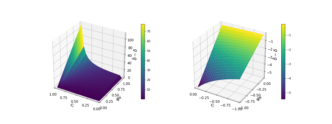
Refer to caption
Figure 1: The plot of δ¯i−δi\bar{\delta}_{i}-\delta_{i} versus cic_{i} and ψN\psi_{N}, with N=25N=25 and φN=6\varphi_{N}=6.

2.1.1 The Markovian case

We consider a single stochastic factor model in which the stock price process (St)t∈[0,T]\left(S_{t}\right)_{t\in\left[0,T\right]} solves

d​St\displaystyle\,dS_{t} =μ⁡(t,Yt)​St​d​t+σ⁡(t,Yt)​St​d​Wt,\displaystyle=\mu(t,Y_{t})S_{t}\,dt+\sigma(t,Y_{t})S_{t}\,dW_{t}, (2.24)
d​Yt\displaystyle\,dY_{t} =b⁡(t,Yt)​d​t+a⁡(t,Yt)​d​WtY,\displaystyle=b(t,Y_{t})\,dt+a(t,Y_{t})\,dW_{t}^{Y}, (2.25)

with S0=S>0S_{0}=S>0 and Y0=y∈ℝY_{0}=y\in\mathbb{R}. The market coefficients μ,σ,a\mu,\sigma,a and bb satisfy appropriate conditions for these equations to have a unique strong solution. Further conditions, added next, are needed for the validity of the Feynman-Kac formula in Proposition 2.7.

Assumption 2.6.

The coefficients μ,σ,a\mu,\sigma,a and bb are bounded functions, and a,ba,b have bounded, uniformly in tt, yy-derivatives. It is further assumed that the Sharpe ratio function λ⁡(t,y):=μ⁡(t,y)σ⁡(t,y)\lambda(t,y):=\frac{\mu\left(t,y\right)}{\sigma\left(t,y\right)} is bounded and with bounded, uniformly in tt, yy-derivatives of any order.

For t∈[0,T],t\in\left[0,T\right], we consider the optimization problem

Vi​(t,x1,…,xi,…,xN,y)=supπi∈𝒜Eℙ[−exp(−1δi(XTi−ciCT))|Xt1=x1,…,Xti=xi,…,XtN=xN,Yt=y],V^{i}(t,x_{1},\ldots,x_{i},\ldots,x_{N},y)\\ =\sup_{\pi^{i}\in\mathcal{A}}E_{\mathbb{P}}\left[\left.-\exp\left(-\frac{1}{\delta_{i}}\left(X_{T}^{i}-c_{i}C_{T}\right)\right)\right|X_{t}^{1}=x_{1},\ldots,X_{t}^{i}=x_{i},\ldots,X_{t}^{N}=x_{N},Y_{t}=y\right], (2.26)

with (Xsi)s∈[t,T](X^{i}_{s})_{s\in\left[t,T\right]} solving d​Xsi=μ⁡(s,Ys)​πsi​d​s+σ⁡(s,Ys)​πsi​d​WsdX_{s}^{i}=\mu(s,Y_{s})\pi_{s}^{i}\,ds+\sigma(s,Y_{s})\pi_{s}^{i}\,dW_{s} and πi∈𝒜,\pi^{i}\in\mathcal{A}, and CTC_{T} as in (2.5). We also consider the process (ζt)t∈[0,T](\zeta_{t})_{t\in\left[0,T\right]} with ζt:=ζ⁡(t,Yt)\zeta_{t}:=\zeta(t,Y_{t}), where ζ:[0,T]×ℝ→ℝ+\zeta:\left[0,T\right]\times\mathbb{R\rightarrow R}^{+} is defined as

ζ(t,y)=EℚM​M[e−12(1−ρ2)∫tTλ2(s,Ys)ds|Yt=y].\zeta(t,y)=E_{\mathbb{Q}^{MM}}\left[\left.e^{-\frac{1}{2}(1-\rho^{2})\int_{t}^{T}\lambda^{2}(s,Y_{s})\,ds}\right|Y_{t}=y\right].

Under ℚM​M\mathbb{Q}^{MM}, the stochastic factor process (Yt)t∈[0,T]\left(Y_{t}\right)_{t\in\left[0,T\right]} satisfies

d​Yt=(b⁡(t,Yt)−ρ​λ​(t,Yt)​a​(t,Yt))​d​t+a⁡(t,Yt)​d​W~tY.\,dY_{t}=(b(t,Y_{t})-\rho\lambda(t,Y_{t})a(t,Y_{t}))\,dt+a(t,Y_{t})\,d\widetilde{W}_{t}^{Y}.

Thus, using the conditions on the market coefficients and the Feynman-Kac formula, we deduce that ζ⁡(t,y)\zeta(t,y) solves

ζt+12​a2​(t,y)​ζy​y+(b⁡(t,y)−ρ​λ​(t,y)​a​(t,y))​ζy=12​(1−ρ2)​λ2​(t,y)​ζ,\zeta_{t}+\frac{1}{2}a^{2}(t,y)\zeta_{yy}+(b(t,y)-\rho\lambda(t,y)a(t,y))\zeta_{y}=\frac{1}{2}(1-\rho^{2})\lambda^{2}(t,y)\zeta, (2.27)

with ζ⁡(T,y)=1.\zeta(T,y)=1. In turn, the function f⁡(t,y):=11−ρ2​ln⁡ζ⁡(t,y)f(t,y):=\frac{1}{1-\rho^{2}}\ln\zeta(t,y) satisfies

ft+12a2(t,y)fy​y+(b(t,y)−ρλ(t,y)a(t,y))fy+12(1−ρ2)a2(t,y)fy=212λ2(t,y),f(T,y)=0.f_{t}+\frac{1}{2}a^{2}(t,y)f_{yy}+(b(t,y)-\rho\lambda(t,y)a(t,y))f_{y}+\frac{1}{2}(1-\rho^{2})a^{2}(t,y)f_{y}{}^{2}=\frac{1}{2}\lambda^{2}(t,y),\quad f(T,y)=0. (2.28)

In the absence of competitive/homophilous interaction, this problem has been examined by various authors (see, for example, [18]).

Proposition 2.7.

Under Assumption 2.6, the following assertions hold for t∈[0,T].t\in\left[0,T\right].

  1. 1.

    If ψN<1\psi_{N}<1, there exists a wealth-independent Nash equilibrium (πs∗)s∈[t,T]=(πs1,∗,…,πsi,∗,…,πsN,∗)s∈[t,T],\left(\pi^{\ast}_{s}\right)_{{}_{s\in\left[t,T\right]}}=\left(\pi^{1,\ast}_{s},\ldots,\pi^{i,\ast}_{s},\ldots,\pi^{N,\ast}_{s}\right)_{{}_{s\in\left[t,T\right]}}, where πsi,∗\pi_{s}^{i,\ast}, i∈ℐi\in\mathcal{I}, is given by the process

    πsi,∗=πi,∗​(s,Ys),\pi_{s}^{i,\ast}=\pi^{i,\ast}(s,Y_{s}), (2.29)

    with (Yt)t∈[0,T](Y_{t})_{t\in[0,T]} solving (2.25) and πi,∗:[0,T]×ℝ→ℝ\pi^{i,\ast}:\left[0,T\right]\times\mathbb{R\rightarrow R} defined as

    πi,∗​(t,y):=δ¯i​(λ⁡(t,y)σ⁡(t,y)+ρ​a⁡(t,y)σ⁡(t,y)​fy​(t,y)),\pi^{i,\ast}(t,y):=\bar{\delta}_{i}\left(\frac{\lambda(t,y)}{\sigma(t,y)}+\rho\frac{a(t,y)}{\sigma(t,y)}f_{y}(t,y)\right), (2.30)

    with δ¯i\bar{\delta}_{i} as in (2.16) and f⁡(t,y)f(t,y) solving (2.28). The game value of player ii, i∈ℐi\in\mathcal{I}, is given by

    Vi​(t,x1,…,xN,y)\displaystyle V^{i}(t,x_{1},\ldots,x_{N},y) =−exp⁡(−1δi​(xi−ciN​Σi=1N​xi))​ζ​(t,y)11−ρ2\displaystyle=-\exp\left(-\frac{1}{\delta_{i}}\left(x_{i}-\frac{c_{i}}{N}\Sigma_{i=1}^{N}x_{i}\right)\right)\zeta(t,y)^{\frac{1}{1-\rho^{2}}}
    =−exp⁡(−1δi​(xi−ciN​Σi=1N​xi)+f⁡(t,y)).\displaystyle=-\exp\left(-\frac{1}{\delta_{i}}\left(x_{i}-\frac{c_{i}}{N}\Sigma_{i=1}^{N}x_{i}\right)+f\left(t,y\right)\right).
  2. 2.

    If ψN=1\psi_{N}=1, there exists no such Nash equilibrium.

Proof.

To ease the notation, we establish the results when t=0t=0 in (2.26). To this end, we first identify the process ξ\xi in (2.10). For this, we rewrite the martingale in (2.9) as

Mt=ζ(t,Yt)e−12(1−ρ2)∫0tλ2(s,Ys)ds,M_{t}=\zeta(t,Y_{t})e^{-\frac{1}{2}(1-\rho^{2})\int_{0}^{t}\lambda^{2}(s,Y_{s})\,ds},

and observe that

d​Mt\displaystyle\,dM_{t} =(ζt​(t,Yt)+(b⁡(t,Yt)−ρ​a​(t,Yt)​λ​(t,Yt))​ζy​(t,Yt)+12​a2​(t,Yt)​ζy​y​(t,Yt))​Mtζ⁡(t,Yt)​d​t\displaystyle=\left(\zeta_{t}(t,Y_{t})+(b(t,Y_{t})-\rho a(t,Y_{t})\lambda(t,Y_{t}))\zeta_{y}(t,Y_{t})+\frac{1}{2}a^{2}(t,Y_{t})\zeta_{yy}(t,Y_{t})\right)\frac{M_{t}}{\zeta(t,Y_{t})}\,dt
−12​(1−ρ2)​λ2​(t,Yt)​Mt​d​t+a⁡(t,Yt)​ζy​(t,Yt)ζ⁡(t,Yt)​Mt​(ρ​d​W~t+1−ρ2​d​Wt⟂)\displaystyle\qquad-\frac{1}{2}(1-\rho^{2})\lambda^{2}(t,Y_{t})M_{t}\,dt+a(t,Y_{t})\frac{\zeta_{y}(t,Y_{t})}{\zeta(t,Y_{t})}M_{t}\left(\rho\,d\widetilde{W}_{t}+\sqrt{1-\rho^{2}}\,dW_{t}^{\perp}\right) (2.31)
=a⁡(t,Yt)​ζy​(t,Yt)ζ⁡(t,Yt)​Mt​(ρ​d​W~t+1−ρ2​d​Wt⟂),\displaystyle=a(t,Y_{t})\frac{\zeta_{y}(t,Y_{t})}{\zeta(t,Y_{t})}M_{t}\left(\rho\,d\widetilde{W}_{t}+\sqrt{1-\rho^{2}}\,dW_{t}^{\perp}\right), (2.32)

where we used that ζ⁡(t,y)\zeta(t,y) satisfies (2.27). Therefore, ξt=a⁡(t,Yt)​ζy​(t,Yt)ζ⁡(t,Yt)\xi_{t}=a(t,Y_{t})\frac{\zeta_{y}(t,Y_{t})}{\zeta(t,Y_{t})}. In turn, using that ζ​(t,y)1/(1−ρ2)=ef⁡(t,y),\zeta(t,y)^{1/(1-\rho^{2})}=e^{f(t,y)}, we obtain that

fy​(t,Yt)=11−ρ2​ζy​(t,y)ζ⁡(t,y)​ and ​ξt=(1−ρ2)​a​(t,Yt)​fy​(t,Yt),f_{y}(t,Y_{t})=\frac{1}{1-\rho^{2}}\frac{\zeta_{y}(t,y)}{\zeta(t,y)}\text{ \ \ and \ \ }\xi_{t}=(1-\rho^{2})a(t,Y_{t})f_{y}(t,Y_{t}),

and we easily conclude by replacing ξt\xi_{t} by (1−ρ2)​a​(t,Yt)​fy​(t,Yt)(1-\rho^{2})a(t,Y_{t})f_{y}(t,Y_{t}) in (2.17).

It remains to show that the candidate investment process in (2.29) is admissible. Under Assumption 2.6 we deduce that fy​(t,y)f_{y}(t,y) is a bounded function, since ζ⁡(t,y)\zeta(t,y) is bounded away from zero and ζy​(t,y)\zeta_{y}(t,y) is bounded. We easily conclude. ∎

Remark 2.8.

In the Markovian model (2.24)–(2.25), the density of the minimal entropy measure ℚM​E\mathbb{Q}^{ME} is fully specified. Indeed, the BSDE (2.23) admits the solution

yt=f(t,Yt),Zt=ρa(t,Yt)fy(t,Yt) and Zt⟂=1−ρ2a(t,Yt)fy(t,Yt),y_{t}=f(t,Y_{t}),\quad Z_{t}=\rho a(t,Y_{t})f_{y}(t,Y_{t})\text{ \ \ and \ \ }Z_{t}^{\perp}=\sqrt{1-\rho^{2}}a(t,Y_{t})f_{y}(t,Y_{t}),

and, thus, the density of ℚM​E\mathbb{Q}^{ME} is given by (2.22) with χt≡χ⁡(t,Yt)=−1−ρ2​a​(t,Yt)​fy​(t,Yt)\chi_{t}\equiv\chi(t,Y_{t})=-\sqrt{1-\rho^{2}}a(t,Y_{t})f_{y}(t,Y_{t}).

2.1.2 A fully solvable example

Consider the family of models with autonomous dynamics

μ(t,y)=μy12​ℓ+12, σ(t,y)=y12​ℓ, b(t,y)=m−y,a(t,y)=βy, \mu(t,y)=\mu y^{\frac{1}{2\ell}+\frac{1}{2}}\text{, \ }\sigma(t,y)=y^{\frac{1}{2\ell}},\text{ \ }b(t,y)=m-y,\quad a(t,y)=\beta\sqrt{y},\text{\ }

with μ>0,\mu>0, β>0,\beta>0, ℓ≠0\ell\neq 0 and m>12​β2m>\frac{1}{2}\beta^{2}. Notable cases are ℓ=1,\ell=1, which corresponds to the Heston stochastic volatility model, and ℓ=−1\ell=-1 that is studied in [3].

Equation (2.28) depends only on b⁡(t,y)b(t,y), a⁡(t,y)a(t,y) and the Sharpe ratio λ⁡(t,y)=\lambda(t,y)= μ​y\mu\sqrt{y}, and thus its solution f⁡(t,y)f(t,y) is independent of the parameter ℓ\ell. Using the ansatz f⁡(t,y)=p⁡(t)​y+q⁡(t)f(t,y)=p(t)y+q(t) with p⁡(T)=q⁡(T)=0p(T)=q(T)=0, we deduce from (2.28) that p⁡(t)p(t) and q⁡(t)q(t) satisfy

p˙​(t)−12​(μ+ρ​β​p​(t))2−p⁡(t)+12​β2​p2​(t)=0,\displaystyle\dot{p}(t)-\frac{1}{2}(\mu+\rho\beta p(t))^{2}-p(t)+\frac{1}{2}\beta^{2}p^{2}(t)=0,
q˙​(t)+m​p​(t)=0.\displaystyle\dot{q}(t)+mp(t)=0. (2.33)

In turn,

p⁡(t)=1+ρ​μ​β−Δ(1−ρ2)​β2​1−e−Δ​(T−t)1−1+ρ​μ​β−Δ1+ρ​μ​β+Δ​e−Δ​(T−t),Δ=1+β2​μ2+2​ρ​μ​β>0,p(t)=\frac{1+\rho\mu\beta-\sqrt{\Delta}}{(1-\rho^{2})\beta^{2}}\frac{1-e^{-\sqrt{\Delta}(T-t)}}{1-\frac{1+\rho\mu\beta-\sqrt{\Delta}}{1+\rho\mu\beta+\sqrt{\Delta}}e^{-\sqrt{\Delta}(T-t)}},\quad\Delta=1+\beta^{2}\mu^{2}+2\rho\mu\beta>0,

and q⁡(t)=m​∫tTp⁡(s)​𝑑sq(t)=m\int_{t}^{T}p(s)ds.

From (2.30), we obtain that the Nash equilibrium strategy (πsi,∗)s∈[t,T],\left(\pi_{s}^{i,\ast}\right)_{s\in\left[t,T\right]}, t∈[0,T],t\in\left[0,T\right], for player ii is given by the process

πsi,∗=δ¯i​(μ+ρ​β​p​(s))​Ys12​(1−1ℓ).\pi_{s}^{i,\ast}=\bar{\delta}_{i}(\mu+\rho\beta p(s))Y_{s}^{\frac{1}{2}(1-\frac{1}{\ell})}.

If ℓ=1\ell=1, the policy becomes deterministic, πsi,∗=δ¯i​(μ+ρ​β​p​(s)),\pi_{s}^{i,\ast}=\bar{\delta}_{i}(\mu+\rho\beta p(s)), and the equilibrium wealth process solves

d​Xsi,∗=δ¯i​(μ+ρ​β​p​(s))​(μ​Ys​d​s+Ys​d​Ws).\,dX_{s}^{i,\ast}=\overline{\delta}_{i}(\mu+\rho\beta p(s))(\mu Y_{s}\,ds+\sqrt{Y_{s}}\,dW_{s}).

2.2 The common-noise MFG

We analyze the limit as N↑∞N\uparrow\infty of the NN-player game studied in Section 2.1. We first give an intuitive and informal argument that leads to a candidate optimal strategy in the mean-field setting, and then propose a rigorous formulation for the MFG. The analysis follows closely the arguments developed in [12].

For the NN-player game, we denote by ηi=(xi,δi,ci)\eta_{i}=(x_{i},\delta_{i},c_{i}) the type vector for player ii, where xix_{i} is her initial wealth, and ηi\eta_{i} and cic_{i} are her risk tolerance coefficient and interaction parameter, respectively. Such type vectors induce an empirical measure mNm_{N}, called the type distribution,

mN(A)=1N∑i=1N𝟏ηi(A), for Borel sets A⊂𝒵,m_{N}(A)=\frac{1}{N}\sum_{i=1}^{N}\mathbf{1}_{\eta_{i}}(A),\text{ for Borel sets }A\subset\mathcal{Z},

which is a probability measure on the space 𝒵:=ℝ×(0,∞)×(−∞,1]\mathcal{Z}:=\mathbb{R}\times(0,\infty)\times(-\infty,1].

We recall (cf. (2.17)) that the equilibrium strategies (πti,∗)t∈[0,T](\pi_{t}^{i,\ast})_{t\in\left[0,T\right]}, i∈ℐi\in\mathcal{I}, are given as the product of the common (type-independent) process λtσt+ρ1−ρ2​ξtσt\frac{\lambda_{t}}{\sigma_{t}}+\frac{\rho}{1-\rho^{2}}\frac{\xi_{t}}{\sigma_{t}} and the modified risk tolerance parameter δ¯i=δi+φN1−ψN​ci\bar{\delta}_{i}=\delta_{i}+\frac{\varphi_{N}}{1-\psi_{N}}c_{i}. Therefore, it is only the coefficient δ¯i\bar{\delta}_{i} that depends on the empirical distribution mNm_{N} through ψN\psi_{N} and φN\varphi_{N}, as both these quantities can be obtained by averaging appropriate functions over mNm_{N}. Therefore, if we assume that mNm_{N} converges weakly to some limiting probability measure as N↑∞N\uparrow\infty, we should intuitively expect that the corresponding equilibrium strategies also converge. This is possible, for instance, by letting the type vector η=(x,δ,c)\eta=(x,\delta,c) be a random variable in the space 𝒵\mathcal{Z} with limiting distribution mm, and take ηi\eta_{i} as i.i.d. samples of η\eta. The sample ηi\eta_{i} is drawn and assigned to player ii at initial time t=0.t=0. We would then expect (πi,∗)t∈[0,T](\pi^{i,\ast})_{t\in\left[0,T\right]} to converge to the process

limN↑∞πti,∗=(δi+δ¯1−c¯​ci)​(λtσt+ρ1−ρ2​ξtσt),\lim_{N\uparrow\infty}\pi_{t}^{i,\ast}=\left(\delta_{i}+\frac{\bar{\delta}}{1-\bar{c}}c_{i}\right)\left(\frac{\lambda_{t}}{\sigma_{t}}+\frac{\rho}{1-\rho^{2}}\frac{\xi_{t}}{\sigma_{t}}\right), (2.34)

where c¯\bar{c} and δ¯\bar{\delta} represent the average interaction and risk tolerance coefficients.

Next, we introduce the mean-field game in the incomplete Itô-diffusion market herein, and we show that (2.34) indeed arises as its equilibrium strategy. We model a single representative player, whose type vector is a random variable with distribution mm, and all players in the continuum act in this common incomplete market.

2.2.1 The Itô-diffusion common-noise MFG

To describe the heterogeneous population of players, we introduce the type vector

η=(x,δ,c)∈𝒵,\eta=(x,\delta,c)\in\mathcal{Z}, (2.35)

where δ>0\delta>0 and c∈(−∞,1]c\in\left(-\infty,1\right] represent the risk tolerance coefficient and interaction parameter, and xx is the initial wealth. This type vector is assumed to be independent of both WW and WYW^{Y}, which drive the stock price process (2.1), and is assumed to have finite second moments.

To formulate the mean-field portfolio game, we now let the filtered probability space (Ω,ℱ,ℙ)(\Omega,\mathcal{F},\mathbb{P}) support W,W, WYW^{Y} as well as η\eta. We assume that η\eta has second moments under ℙ\mathbb{P}. We denote by (ℱtM​F)t∈[0,T](\mathcal{F}_{t}^{MF})_{t\in[0,T]} the smallest filtration satisfying the usual assumptions for which η\eta is ℱ0M​F\mathcal{F}_{0}^{MF}-measurable and both W,WYW,W^{Y} are adapted. As before, we denote by (ℱt)t∈[0,T](\mathcal{F}_{t})_{t\in[0,T]} the natural filtration generated by WW and WY,W^{Y}, and by (𝒢t)t∈[0,T](\mathcal{G}_{t})_{t\in[0,T]} the one generated only by WY.W^{Y}.

We also consider the wealth process (Xt)t∈[0,T]\left(X_{t}\right)_{t\in\left[0,T\right]} of the representative player solving

d​Xt=πt​(μt​d​t+σt​d​Wt),\,dX_{t}=\pi_{t}\left(\mu_{t}\,dt+\sigma_{t}\,dW_{t}\right), (2.36)

with X0=x∈ℝX_{0}=x\in\mathbb{R} and π\pi ∈𝒜M​F\in\mathcal{A}^{MF}, where

𝒜M​F={π:self-financing, ​ℱtM​F​-progressively measurable and ​Eℙ​[∫0Tσs2​πs2​𝑑s]<∞}.\mathcal{A}^{MF}=\left\{\pi:\text{self-financing, }\mathcal{F}_{t}^{MF}\text{-progressively measurable and }E_{\mathbb{P}}\left[\int_{0}^{T}\sigma_{s}^{2}\pi_{s}^{2}\,ds\right]<\infty\right\}.

Similarly to the framework in [12], there exist two independent sources of randomness in the model: the first is due to the evolution of the stock price process, described by the Brownian motions WW and WYW^{Y}. The second is given by η\eta, which models the type of the player, i.e., the triplet of initial wealth, risk tolerance, and interaction parameter in the population continuum. The first source of noise is stochastic and common to each player in the continuum while the second is static, being assigned at time zero and with the dynamic competition starting right afterwards.

In analogy to the NN-player setting, the representative player optimizes the expected terminal utility, taking into account the performance of the average terminal wealth of the population, denoted by X¯.\overline{X}. As in [12], we introduce the following definition for the MFG considered herein.

Definition 2.9.

For each π∈𝒜M​F\pi\in\mathcal{A}^{MF}, let X¯:=Eℙ​[XT|ℱT]\overline{X}:=E_{\mathbb{P}}[X_{T}|\mathcal{F}_{T}] with (Xt)t∈[0,T]\left(X_{t}\right)_{t\in\left[0,T\right]} solving (2.36), and consider the optimization problem

V(x)=supπ∈𝒜M​FEℙ[−exp(−1δ(XT−cX¯))|ℱ0M​F,X0=x].V(x)=\sup_{\pi\in\mathcal{A}^{MF}}E_{\mathbb{P}}\left[\left.-\exp\left(-\frac{1}{\delta}\left(X_{T}-c\overline{X}\right)\right)\right|\mathcal{F}_{0}^{MF},X_{0}=x\right]. (2.37)

A strategy π∗∈𝒜M​F\mathit{\ }\pi^{\ast}\in\mathcal{A}^{MF} is a mean-field equilibrium if π∗\pi^{\ast} is the optimal strategy of the above problem when X¯∗:=Eℙ​[XT∗|ℱT]\overline{X}^{\ast}:=E_{\mathbb{P}}[X_{T}^{\ast}|\mathcal{F}_{T}] is used for X¯\overline{X}, where (Xt∗)t∈[0,T]\left(X_{t}^{\ast}\right)_{t\in\left[0,T\right]} solves (2.36) with π∗\pi^{\ast} being used.

Next, we state the main result.

Proposition 2.10.

If Eℙ​[c]<1E_{\mathbb{P}}[c]<1, there exists a unique wealth-independent MFG equilibrium (πt∗)t∈[0,T]\left(\pi_{t}^{\ast}\right)_{t\in\left[0,T\right]}, given by the ℱ0M​F∨𝒢t\mathcal{F}_{0}^{MF}\vee\mathcal{G}_{t} process

πt∗=(δ+Eℙ​[δ]1−Eℙ​[c]​c)​(λtσt+ρ1−ρ2​ξtσt),\pi_{t}^{\ast}=\left(\delta+\frac{E_{\mathbb{P}}[\delta]}{1-E_{\mathbb{P}}[c]}c\right)\left(\frac{\lambda_{t}}{\sigma_{t}}+\frac{\rho}{1-\rho^{2}}\frac{\xi_{t}}{\sigma_{t}}\right), (2.38)

with ξ\xi as in (2.10). The corresponding optimal wealth is given by

Xt∗=x+(δ+Eℙ​[δ]1−Eℙ​[c]​c)​∫0t(λs+ρ1−ρ2​ξs)​(λs​𝑑s+d​Ws),X_{t}^{\ast}=x+\left(\delta+\frac{E_{\mathbb{P}}[\delta]}{1-E_{\mathbb{P}}[c]}c\right)\int_{0}^{t}\left(\lambda_{s}+\frac{\rho}{1-\rho^{2}}\xi_{s}\right)\left(\lambda_{s}\,ds+\,dW_{s}\right), (2.39)

and

V(x)=−exp(−1δ(x−cm))M011−ρ2=−exp(−1δ(x−cm))(EℚM​M[e−12(1−ρ2)∫0Tλs2ds])11−ρ2,V(x)=-\exp\left(-\frac{1}{\delta}\left(x-cm\right)\right)M_{0}^{\frac{1}{1-\rho^{2}}}=-\exp\left(-\frac{1}{\delta}\left(x-cm\right)\right)\left(E_{\mathbb{Q}^{MM}}\left[e^{-\frac{1}{2}(1-\rho^{2})\int_{0}^{T}\lambda_{s}^{2}\,ds}\right]\right)^{\frac{1}{1-\rho^{2}}},

where m=Eℙ​[x]m=E_{\mathbb{P}}[x]. If Eℙ​[c]=1E_{\mathbb{P}}[c]=1, there is no such Nash equilibrium.

Proof.

We first observe that π∗\pi^{\ast} in (2.38) is ℱtM​F\mathcal{F}_{t}^{MF}-measurable since (λtσt+ρ1−ρ2​ξtσt)∈\left(\frac{\lambda_{t}}{\sigma_{t}}+\frac{\rho}{1-\rho^{2}}\frac{\xi_{t}}{\sigma_{t}}\right)\in 𝒢t\mathcal{G}_{t}, and thus
(λtσt+ρ1−ρ2​ξtσt)∈ℱt\left(\frac{\lambda_{t}}{\sigma_{t}}+\frac{\rho}{1-\rho^{2}}\frac{\xi_{t}}{\sigma_{t}}\right)\in\mathcal{F}_{t}, while the factor (δ+Eℙ​[δ]1−Eℙ​[c]​c)∈ℱ0M​F\left(\delta+\frac{E_{\mathbb{P}}[\delta]}{1-E_{\mathbb{P}}[c]}c\right)\in\mathcal{F}_{0}^{MF} (independent of ℱt\mathcal{F}_{t}). Furthermore, π∗\pi^{\ast} is also square-integrable under standing assumptions, and thus admissible. To show that it is also indeed an equilibrium policy, we shall first define X¯\overline{X} using π∗\pi^{\ast}, and then verify that the optimal strategy to the representative player’s problem (2.37) coincides with πt∗\pi_{t}^{\ast} when this specific X¯\overline{X} is used in (2.37). To this end, we introduce the process X¯t:=Eℙ​[Xt∗|ℱt]\overline{X}_{t}:=E_{\mathbb{P}}[X_{t}^{\ast}|\mathcal{F}_{t}] with (Xt∗)t∈[0,T](X_{t}^{\ast})_{t\in[0,T]} as in (2.39). Then,

X¯t\displaystyle\overline{X}_{t} =Eℙ​[x+(δ+Eℙ​[δ]1−Eℙ​[c]​c)​∫0t(λs+ρ1−ρ2​ξs)​(λs​𝑑s+d​Ws)|ℱt]\displaystyle=E_{\mathbb{P}}\left[x+\left(\delta+\frac{E_{\mathbb{P}}[\delta]}{1-E_{\mathbb{P}}[c]}c\right)\int_{0}^{t}\left(\lambda_{s}+\frac{\rho}{1-\rho^{2}}\xi_{s}\right)\left(\lambda_{s}\,ds+\,dW_{s}\right)\Big|\mathcal{F}_{t}\right]
=m+(Eℙ​[δ]+Eℙ​[δ]1−Eℙ​[c]​Eℙ​[c])​∫0t(λs+ρ1−ρ2​ξs)​(λs​𝑑s+d​Ws)\displaystyle=m+\left(E_{\mathbb{P}}[\delta]+\frac{E_{\mathbb{P}}[\delta]}{1-E_{\mathbb{P}}[c]}E_{\mathbb{P}}[c]\right)\int_{0}^{t}\left(\lambda_{s}+\frac{\rho}{1-\rho^{2}}\xi_{s}\right)\left(\lambda_{s}\,ds+\,dW_{s}\right)
=m+(Eℙ​[δ]1−Eℙ​[c])​∫0t(λs+ρ1−ρ2​ξs)​(λs​𝑑s+d​Ws),\displaystyle=m+\left(\frac{E_{\mathbb{P}}[\delta]}{1-E_{\mathbb{P}}[c]}\right)\int_{0}^{t}\left(\lambda_{s}+\frac{\rho}{1-\rho^{2}}\xi_{s}\right)\left(\lambda_{s}\,ds+\,dW_{s}\right),

where we have used that ∫0t(λs+ρ1−ρ2​ξs)​(λs​𝑑s+d​Ws)\int_{0}^{t}\left(\lambda_{s}+\frac{\rho}{1-\rho^{2}}\xi_{s}\right)\left(\lambda_{s}\,ds+\,dW_{s}\right) is 𝒢t\mathcal{G}_{t}-measurable and thus ℱt\mathcal{F}_{t}-measurable, and that (δ+Eℙ​[δ]1−Eℙ​[c]​c)\left(\delta+\frac{E_{\mathbb{P}}[\delta]}{1-E_{\mathbb{P}}[c]}c\right) is independent of ℱt\mathcal{F}_{t}.

Next, we introduce the auxiliary process (x~t)t∈[0,T]\left(\tilde{x}_{t}\right)_{t\in\left[0,T\right]}, x~t:=Xt−c​X¯t,\,\tilde{x}_{t}:=\,X_{t}-c\overline{X}_{t}, with (Xt)t∈[0,T]\left(X_{t}\right)_{t\in\left[0,T\right]} as in (2.36). Then,

d​x~t=π~t​(μt​d​t+σt​d​Wt)​ and ​x~0=x~:=x−c​m,d\tilde{x}_{t}=\widetilde{\pi}_{t}(\mu_{t}\,dt+\sigma_{t}\,dW_{t})\text{ \ \ and \ \ }\,\tilde{x}_{0}=\tilde{x}:=x-cm,

and π~t=πt−c⁡(Eℙ​[δ]1−Eℙ​[c])​(λtσt+ρ1−ρ2​ξtσt)\widetilde{\pi}_{t}=\pi_{t}-c\left(\frac{E_{\mathbb{P}}[\delta]}{1-E_{\mathbb{P}}[c]}\right)\left(\frac{\lambda_{t}}{\sigma_{t}}+\frac{\rho}{1-\rho^{2}}\frac{\xi_{t}}{\sigma_{t}}\right). In turn, we consider the optimization problem

v(x~):=supπ~∈𝒜M​FEℙ[−exp(−1δx~T)|ℱ0M​F,x~0=x~].v(\tilde{x}):=\sup_{\widetilde{\pi}\in\mathcal{A}^{MF}}E_{\mathbb{P}}\left[\left.-\exp\left(-\frac{1}{\delta}\tilde{x}_{T}\right)\right|\mathcal{F}_{0}^{MF},\,\tilde{x}_{0}=\tilde{x}\right].

From Lemma 2.2, we deduce that the optimal strategy is given by

π~t∗=δ⁡(λtσt+ρ1−ρ2​ξtσt),\widetilde{\pi}_{t}^{\ast}=\delta\left(\frac{\lambda_{t}}{\sigma_{t}}+\frac{\rho}{1-\rho^{2}}\frac{\xi_{t}}{\sigma_{t}}\right),

and, thus,

πt∗=δ⁡(λtσt+ρ1−ρ2​ξtσt)+c⁡(Eℙ​[δ]1−Eℙ​[c])​(λtσt+ρ1−ρ2​ξtσt).\pi_{t}^{\ast}=\delta\left(\frac{\lambda_{t}}{\sigma_{t}}+\frac{\rho}{1-\rho^{2}}\frac{\xi_{t}}{\sigma_{t}}\right)+c\left(\frac{E_{\mathbb{P}}[\delta]}{1-E_{\mathbb{P}}[c]}\right)\left(\frac{\lambda_{t}}{\sigma_{t}}+\frac{\rho}{1-\rho^{2}}\frac{\xi_{t}}{\sigma_{t}}\right).

The rest of the proof follows easily. ∎

If we view η=(x,δ,c)\eta=(x,\delta,c) in the NN-player game in Section 2.1 as i.i.d. samples on the space 𝒵\mathcal{Z} with distribution mm, then limN↑∞ψN=Eℙ​[c]\lim_{N\uparrow\infty}\psi_{N}=E_{\mathbb{P}}[c] and limN↑∞φN=Eℙ​[δ]\lim_{N\uparrow\infty}\varphi_{N}=E_{\mathbb{P}}[\delta] a.s.. We then obtain the convergence of the corresponding optimal processes, namely, for t∈[0,T]t\in\left[0,T\right],

limN↑∞πti,∗=πt∗, and ​limN↑∞Xti,∗=Xt∗.\lim_{N\uparrow\infty}\pi_{t}^{i,\ast}=\pi_{t}^{\ast},\text{ \ \ and \ }\lim_{N\uparrow\infty}X_{t}^{i,\ast}=X_{t}^{\ast}.

2.2.2 The Markovian case

In analogy to the NN-player case, we have the following result.

Proposition 2.11.

Assume that the stock price process follows the single factor model (2.24)–(2.25). Then, if Eℙ​[c]<1,E_{\mathbb{P}}[c]<1, there exists a unique wealth-independent Markovian mean-field game equilibrium, given by the process (πt∗)t∈[0,T],\left(\pi_{t}^{\ast}\right)_{t\in\left[0,T\right]},

πt∗=π∗​(η,t,Yt)=(δ+Eℙ​[δ]1−Eℙ​[c]​c)​(λ⁡(t,Yt)σ⁡(t,Yt)+ρ​a⁡(t,Yt)σ⁡(t,Yt)​fy​(t,Yt)),\pi_{t}^{\ast}=\pi^{\ast}(\eta,t,Y_{t})=\left(\delta+\frac{E_{\mathbb{P}}[\delta]}{1-E_{\mathbb{P}}[c]}c\right)\left(\frac{\lambda(t,Y_{t})}{\sigma(t,Y_{t})}+\rho\frac{a(t,Y_{t})}{\sigma(t,Y_{t})}f_{y}(t,Y_{t})\right),

with the ℱ0M​F\mathcal{F}_{0}^{MF}-measurable random function π∗​(η,t,y):𝒵×[0,T]×ℝ,\pi^{\ast}(\eta,t,y):\mathcal{Z}\times\left[0,T\right]\times\mathbb{R},

π∗​(η,t,y):=(δ+Eℙ​[δ]1−Eℙ​[c]​c)​(λ⁡(t,y)σ⁡(t,y)+ρ​a⁡(t,y)σ⁡(t,y)​fy​(t,y)).\pi^{\ast}(\eta,t,y):=\left(\delta+\frac{E_{\mathbb{P}}[\delta]}{1-E_{\mathbb{P}}[c]}c\right)\left(\frac{\lambda(t,y)}{\sigma(t,y)}+\rho\frac{a(t,y)}{\sigma(t,y)}f_{y}(t,y)\right).

If Eℙ​[c]=1E_{\mathbb{P}}[c]=1, there is no such mean-field game stochastic equilibrium.

3 Complete Itô-diffusion common market and CARA utilities with random risk tolerance coefficients

In this section, we focus on the complete common market case, but we extend the model by allowing random individual risk tolerance coefficients. We start with a background result for the single-player problem, which is new and interesting in its own right. Building on it, we analyze both the NN-player and the MFG. The analysis shows that the randomness of the individual risk tolerance gives rise to virtual “personalized” markets, in that the original common risk premium process now differs across players, depending on their risk tolerance. This brings substantial complexity as the tractability coming from the original common market is now lost.

3.1 The Itô-diffusion market and random risk tolerance coefficients

We consider the complete analog of the Itô-diffusion market studied in Section 2. Specifically, we consider a market with a riskless bond (taken to be the numeraire and offering zero interest rate) and a stock whose price process (St)t∈[0,T]\left(S_{t}\right)_{t\in\left[0,T\right]} solves

d​St=St​(μt​d​t+σt​d​Wt),dS_{t}=S_{t}\left(\mu_{t}\,dt+\sigma_{t}\,dW_{t}\right),

with S0>0S_{0}>0, and (Wt)t∈[0,T]\left(W_{t}\right)_{t\in\left[0,T\right]} being a Brownian motion in a probability space (Ω,ℱ,ℙ)(\Omega,\mathcal{F},\mathbb{P}). The market coefficients (μt)t∈[0,T]\left(\mu_{t}\right)_{t\in\left[0,T\right]} and (σt)t∈[0,T]\left(\sigma_{t}\right)_{t\in\left[0,T\right]} are ℱt\mathcal{F}_{t}-adapted processes, where (ℱt)t∈[0,T](\mathcal{F}_{t})_{t\in[0,T]} is the natural filtration generated by WW, and with 0<c≤σt≤C0<c\leq\sigma_{t}\leq C and |μt|≤C\left|\mu_{t}\right|\leq C, t∈[0,T]t\in[0,T], for some (possibly deterministic) constants cc and CC.

In this market, NN players, indexed by i∈ℐi\in\mathcal{I}, ℐ={1,2,…,N}\mathcal{I}=\left\{1,2,\ldots,N\right\}, trade between the two accounts in [0,T]\left[0,T\right], with individual wealths (Xti)t∈[0,T]\left(X_{t}^{i}\right)_{t\in\left[0,T\right]} solving

d​Xti=πti​(μt​d​t+σt​d​Wt),\,dX_{t}^{i}=\pi_{t}^{i}\left(\mu_{t}\,dt+\sigma_{t}\,dW_{t}\right), (3.1)

and X0i=xi∈ℝ.X_{0}^{i}=x_{i}\in\mathbb{R}.

Each of the players, say player ii, has random risk tolerance, δTi\delta_{T}^{i}, defined on (Ω,ℱ,ℙ)(\Omega,\mathcal{F},\mathbb{P}) with the following properties:

Assumption 3.1.

For each i∈ℐi\in\mathcal{I}, the risk tolerance δTi\delta_{T}^{i} is an ℱT\mathcal{F}_{T}-measurable random variable with δTi≥δ>0\delta_{T}^{i}\geq\delta>0 and Eℙ​(δTi)2<∞E_{\mathbb{P}}\left(\delta_{T}^{i}\right)^{2}<\infty.

The objective of each player is to optimize

Vi​(x1,…,xi,…,xN)=sup𝒜Eℙ[−exp(−1δTi(XTi−ciN∑j=1NXTj))|X01=x1,…,X0i=xi,…,X0N=xN],V^{i}\left(x_{1},\ldots,x_{i},\ldots,x_{N}\right)\\ =\sup_{\mathcal{A}}E_{\mathbb{P}}\left[\left.-\exp\left(-\frac{1}{\delta_{T}^{i}}\left(X_{T}^{i}-\frac{c_{i}}{N}\sum_{j=1}^{N}X_{T}^{j}\right)\right)\right|X_{0}^{1}=x_{1},\ldots,X_{0}^{i}=x_{i},\ldots,X_{0}^{N}=x_{N}\right], (3.2)

with ci∈(−∞,1]c_{i}\in\left(-\infty,1\right], XjX^{j}, j∈ℐj\in\mathcal{I}, solving (3.1), and 𝒜\mathcal{A} defined similarly to (2.3).

As in Section 2.1, we are interested in a Nash equilibrium solution, which is defined as in Definition 2.1. Before we solve the underlying stochastic NN-player game, we focus on the single-player case. This is a problem interesting in its own right and, to our knowledge, has not been studied before in such markets. A similar problem was considered in a single-period binomial model in [15] and in a special diffusion case in [16] in the context of indifference pricing of bonds. For generality, we present below the time-dependent case.

3.2 The single-player problem

We consider the optimization problem

vt(x)=supπ∈𝒜Eℙ[−e−1δT​xT|ℱt,xt=x],v_{t}(x)=\sup_{\pi\in\mathcal{A}}E_{\mathbb{P}}\left[\left.-e^{-\frac{1}{\delta_{T}}x_{T}}\right|\mathcal{F}_{t},x_{t}=x\right], (3.3)

with δT∈ℱT\delta_{T}\in\mathcal{F}_{T} satisfying Assumption 3.1 and (xs)s∈[t,T]\left(x_{s}\right)_{s\in\left[t,T\right]} solving (3.1) with xt=x∈ℝx_{t}=x\in\mathbb{R}.

We define (Zt)t∈[0,T]\left(Z_{t}\right)_{t\in\left[0,T\right]} by

Zt=exp(−12∫0tλs2ds−∫0tλsdWs),Z_{t}=\exp\left(-\frac{1}{2}\int_{0}^{t}\lambda_{s}^{2}\,ds-\int_{0}^{t}\lambda_{s}\,dW_{s}\right),

and recall the associated (unique) risk neutral measure ℚ\mathbb{Q}, defined on ℱT\mathcal{F}_{T} and given by

d​ℚd​ℙ=ZT.\frac{d\mathbb{Q}}{d\mathbb{P}}=Z_{T}. (3.4)

We introduce the process (δt)t∈[0,T],\left(\delta_{t}\right)_{t\in\left[0,T\right]},

δt:=Eℚ​[δT|ℱt],\delta_{t}:=E_{\mathbb{Q}}[\delta_{T}|\mathcal{F}_{t}], (3.5)

which may be thought as the arbitrage-free price of the risk tolerance “claim” δT\delta_{T}. We also introduce the measure ℚ^\hat{\mathbb{Q}}, defined on ℱT,\mathcal{F}_{T}, with

d​ℚ^d​ℙ=δTEℚ​[δT]​ZT.\frac{d\hat{\mathbb{Q}}}{d\mathbb{P}}=\frac{\delta_{T}}{E_{\mathbb{Q}}[\delta_{T}]}Z_{T}.

Direct calculations yield that under measure ℚ^\hat{\mathbb{Q}}, the process (Stδt)t∈[0,T]\left(\frac{S_{t}}{\delta_{t}}\right)_{t\in\left[0,T\right]} is an ℱt\mathcal{F}_{t}-martingale.

By the model assumptions and the martingale representation theorem, there exists an ℱt\mathcal{F}_{t}-adapted process (ξt)t∈[0,T]\left(\xi_{t}\right)_{t\in\left[0,T\right]} with ξ∈ℒ2​(ℙ)\xi\in\mathcal{L}^{2}\left(\mathbb{P}\right) such that

d​δt=ξt​δt​d​Wtℚ,d\delta_{t}=\xi_{t}\delta_{t}\,dW_{t}^{\mathbb{Q}}, (3.6)

with Wtℚ=Wt+∫0tλs​𝑑sW_{t}^{\mathbb{Q}}=W_{t}+\int_{0}^{t}\lambda_{s}\,ds. Next, we introduce the process

Ht:=Eℚ~[12∫tT(λs−ξs)2ds|ℱt],H_{t}:=E_{\mathbb{\widetilde{Q}}}\left[\left.\frac{1}{2}\int_{t}^{T}\left(\lambda_{s}-\xi_{s}\right)^{2}\,ds\right|\mathcal{F}_{t}\right], (3.7)

where ℚ~\widetilde{\mathbb{Q}} is defined on ℱT\mathcal{F}_{T} by

d​ℚ~d​ℙ=exp(−12∫0T(λs−ξs)2ds−∫0T(λs−ξs)dWs).\frac{d\widetilde{\mathbb{Q}}}{d\mathbb{P}}=\exp\left(-\frac{1}{2}\int_{0}^{T}(\lambda_{s}-\xi_{s})^{2}\,ds-\int_{0}^{T}\left(\lambda_{s}-\xi_{s}\right)\,dW_{s}\right). (3.8)

Under ℚ~\widetilde{\mathbb{Q}}, the process (Wtℚ~)t∈[0,T]\left(W_{t}^{\widetilde{\mathbb{Q}}}\right)_{t\in\left[0,T\right]} with

Wtℚ~:=Wt+∫0t(λs−ξs)​𝑑sW_{t}^{\widetilde{\mathbb{Q}}}:=W_{t}+\int_{0}^{t}\left(\lambda_{s}-\xi_{s}\right)\,ds (3.9)

is a standard Brownian motion, and (1δt​St)t∈[0,T]\left(\frac{1}{\delta_{t}}S_{t}\right)_{t\in[0,T]} is a martingale with dynamics

d⁡(Stδt)=(σt−ξt)​Stδt​d​Wtℚ~.d\left(\frac{S_{t}}{\delta_{t}}\right)=(\sigma_{t}-\xi_{t})\frac{S_{t}}{\delta_{t}}\,dW_{t}^{\widetilde{\mathbb{Q}}}.

Direct calculations yield

d​ℚ~d​ℚ=δT.\frac{d\widetilde{\mathbb{Q}}}{d\mathbb{Q}}=\delta_{T}.

Alternatively, HtH_{t} may be also represented as

Ht=Eℚ​[δT​∫tT12​(λs−ξs)2​𝑑s|ℱt]Eℚ​[δT|ℱt]=Eℚ[δTδt∫tT12(λs−ξs)2ds|ℱt],H_{t}=\frac{E_{\mathbb{Q}}[\delta_{T}\int_{t}^{T}\frac{1}{2}(\lambda_{s}-\xi_{s})^{2}\,ds|\mathcal{F}_{t}]}{E_{\mathbb{Q}}[\delta_{T}|\mathcal{F}_{t}]}=E_{\mathbb{Q}}\left[\frac{\delta_{T}}{\delta_{t}}\int_{t}^{T}\left.\frac{1}{2}(\lambda_{s}-\xi_{s})^{2}\,ds\right|\mathcal{F}_{t}\right], (3.10)

which is obtained by using that

d​ℚ~d​ℚ=exp(−12∫0Tξs2ds+∫0TξsdWsℚ).\frac{d\widetilde{\mathbb{Q}}}{d\mathbb{Q}}=\exp\left(-\frac{1}{2}\int_{0}^{T}\xi_{s}^{2}\,ds+\int_{0}^{T}\xi_{s}\,dW_{s}^{\mathbb{Q}}\right).

Finally, we introduce the processes (Mt)t∈[0,T]\left(M_{t}\right)_{t\in\left[0,T\right]} and (ηt)t∈[0,T]\left(\eta_{t}\right)_{t\in\left[0,T\right]} with

Mt=𝔼ℚ~[12∫0T(λs−ξs)2ds|ℱt] and dMt=ηtdWtℚ~.M_{t}=\mathbb{E}_{\mathbb{\widetilde{Q}}}\left[\frac{1}{2}\int_{0}^{T}\left.\left(\lambda_{s}-\xi_{s}\right)^{2}\,ds\right|\mathcal{F}_{t}\right]\text{ \ \ \ \ and \ \ \ }dM_{t}=\eta_{t}\,dW_{t}^{\widetilde{\mathbb{Q}}}. (3.11)

We are now ready to present the main result.

Proposition 3.2.

The following assertions hold:

  1. 1.

    The value function of (3.3) is given by

    vt​(x)=−exp⁡(−xδt−Ht),v_{t}(x)=-\exp\left(-\frac{x}{\delta_{t}}-H_{t}\right),

    with δ\delta and HH as in (3.5) and (3.7).

  2. 2.

    The optimal strategy (πs∗)s∈[t,T]\left(\pi_{s}^{\ast}\right)_{s\in\left[t,T\right]} is given by

    πs∗=δs​λs−ηs−ξsσs+ξsσs​xs∗,\pi_{s}^{\ast}=\delta_{s}\frac{\lambda_{s}-\eta_{s}-\xi_{s}}{\sigma_{s}}+\frac{\xi_{s}}{\sigma_{s}}x_{s}^{\ast}, (3.12)

    with ξ,η\xi,\eta as in (3.6) and (3.11), and x∗x^{\ast} solving (3.1) with π∗\pi^{\ast} being used.

  3. 3.

    The optimal wealth (xs∗)s∈[t,T]\left(x_{s}^{\ast}\right)_{s\in\left[t,T\right]} solves

    d​xs∗=λs​(δs​(λs−ηs−ξs)+ξs​xs∗)​d​s+(δs​(λs−ηs−ξs)+ξs​xs∗)​d​Ws,xt∗=x,dx_{s}^{\ast}=\lambda_{s}\left(\delta_{s}(\lambda_{s}-\eta_{s}-\xi_{s})+\xi_{s}x_{s}^{\ast}\right)\,ds+\left(\delta_{s}(\lambda_{s}-\eta_{s}-\xi_{s})+\xi_{s}x_{s}^{\ast}\right)\,dW_{s},\quad x_{t}^{\ast}=x,

    and is given by

    xs∗=x​Φt,s+∫tsδu​(λu−ξu)​(λu−ηu−ξu)​Φu,s​𝑑u+∫tsδu​(λu−ηu−ξu)​Φu,s​d​Wu,x_{s}^{\ast}=x\Phi_{t,s}+\int_{t}^{s}\delta_{u}(\lambda_{u}-\xi_{u})(\lambda_{u}-\eta_{u}-\xi_{u})\Phi_{u,s}\,du+\int_{t}^{s}\delta_{u}(\lambda_{u}-\eta_{u}-\xi_{u})\Phi_{u,s}\,dW_{u}, (3.13)

    where, for 0≤u≤s≤T0\leq u\leq s\leq T,

    Φu,s:=exp⁡(∫us(λv−12​ξv)​ξv​𝑑v+∫usξv​d​Wv).\Phi_{u,s}:=\exp\left(\int_{u}^{s}\left(\lambda_{v}-\frac{1}{2}\xi_{v}\right)\xi_{v}\,dv+\int_{u}^{s}\xi_{v}\,dW_{v}\right).

Using (3.13), (3.12) gives the explicit representation of the optimal policy,

πs∗=δs​λs−ηs−ξsσs+ξsσs​(x​Φt,s+∫tsδu​(λu−ξu)​(λu−ηu−ξu)​Φu,s​𝑑u+∫tsδu​(λu−ηu−ξu)​Φu,s​d​Wu).\pi_{s}^{\ast}=\delta_{s}\frac{\lambda_{s}-\eta_{s}-\xi_{s}}{\sigma_{s}}+\frac{\xi_{s}}{\sigma_{s}}\left(x\Phi_{t,s}+\int_{t}^{s}\delta_{u}(\lambda_{u}-\xi_{u})(\lambda_{u}-\eta_{u}-\xi_{u})\Phi_{u,s}\,du+\int_{t}^{s}\delta_{u}(\lambda_{u}-\eta_{u}-\xi_{u})\Phi_{u,s}\,dW_{u}\right).

3.2.1 The Markovian case

We assume that the stock price process (St)t∈[0,T]\left(S_{t}\right)_{t\in\left[0,T\right]} solves

d​St=μ⁡(t,St)​St​d​t+σ⁡(t,St)​St​d​Wt​,dS_{t}=\mu(t,S_{t})S_{t}\,dt+\sigma(t,S_{t})S_{t}\,dW_{t}\text{,}

with the initial price S0>0,S_{0}>0, and the functions μ⁡(t,St)\mu(t,S_{t}) and σ⁡(t,St)\sigma(t,S_{t}) satisfying appropriate conditions, similar to the ones in Subsection 2.1.1 and Assumption 2.6. The risk tolerance is assumed to have the functional representation

δT=δ⁡(ST),\delta_{T}=\delta(S_{T}),

for some function δ:ℝ+→ℝ+\delta:\mathbb{R}^{+}\rightarrow\mathbb{R}^{+} bounded from below and such that Eℙ​[δ2​(ST)]<∞E_{\mathbb{P}}\left[\delta^{2}(S_{T})\right]<\infty, (cf. Assumption 3.1).

The value function in (3.3) takes the form

V(t,x,S)=supπ∈𝒜Eℙ[−e−1δ⁡(ST)​xT|xt=x,St=S],V(t,x,S)=\sup_{\pi\in\mathcal{A}}E_{\mathbb{P}}\left[-e^{-\frac{1}{\delta\left(S_{T}\right)}x_{T}}\Big|x_{t}=x,S_{t}=S\right],

and, in turn, Proposition 3.2 yields

V⁡(t,x,S)=−exp⁡(xδ⁡(t,S)−H⁡(t,S)),V(t,x,S)=-\exp\left(\frac{x}{\delta(t,S)}-H(t,S)\right),

with δ⁡(t,S)\delta(t,S) and H⁡(t,S)H(t,S) solving

δt+12​σ2​(t,S)​S2​δS​S=0,δ⁡(T,S)=δ⁡(S),\delta_{t}+\frac{1}{2}\sigma^{2}(t,S)S^{2}\delta_{SS}=0,\quad\delta(T,S)=\delta(S),

and

Ht+12​σ2​(t,S)​S2​HS​S+1δ⁡(t,S)​σ2​(t,S)​S2​δS​(t,S)​HS+12​(λ⁡(t,S)−1δ⁡(t,S)​σ​(t,S)​S​δS​(t,S))2=0,H⁡(T,S)=0.H_{t}+\frac{1}{2}\sigma^{2}(t,S)S^{2}H_{SS}+\frac{1}{\delta(t,S)}\sigma^{2}(t,S)S^{2}\delta_{S}(t,S)H_{S}+\frac{1}{2}\left(\lambda(t,S)-\frac{1}{\delta(t,S)}\sigma(t,S)S\delta_{S}(t,S)\right)^{2}=0,\quad H(T,S)=0.

Clearly,

δ(t,S)=Eℚ[δ(ST)|St=S],\delta(t,S)=E_{\mathbb{Q}}\left[\left.\delta(S_{T})\right|S_{t}=S\right],

and

H⁡(t,S)=Eℚ~​[∫tT12​(λ⁡(u,Su)−σ⁡(u,Su)​Su​δS​(u,Su)δ⁡(u,Su))2​𝑑u|St=S],H(t,S)=E_{\mathbb{\widetilde{Q}}}\left[\int_{t}^{T}\frac{1}{2}\left(\lambda(u,S_{u})-\sigma(u,S_{u})S_{u}\frac{\delta_{S}(u,S_{u})}{\delta(u,S_{u})}\right)^{2}du\bigg|S_{t}=S\right],

and, furthermore,

ξt=δS​(t,St)δ⁡(t,St)​St​σ​(t,St)​ and ηt=HS​(t,St)​St​σ​(t,St).\xi_{t}=\frac{\delta_{S}(t,S_{t})}{\delta(t,S_{t})}S_{t}\sigma(t,S_{t})\text{ \ \ \ \ and }\quad\eta_{t}=H_{S}(t,S_{t})S_{t}\sigma(t,S_{t}).

Using the above relations and (3.12), we derive the optimal investment process,

πs∗=δ⁡(s,Ss)​(λ⁡(s,Ss)σ⁡(s,Ss)−Ss​HS​(s,Ss))+δS​(s,Ss)​Ss​(−1+1δ⁡(s,Ss)​xs∗).\pi_{s}^{\ast}=\delta(s,S_{s})\left(\frac{\lambda(s,S_{s})}{\sigma(s,S_{s})}-S_{s}H_{S}(s,S_{s})\right)+\delta_{S}(s,S_{s})S_{s}\left(-1+\frac{1}{\delta\left(s,S_{s}\right)}x_{s}^{\ast}\right).

For completeness, we note that if δT≡δ>0\delta_{T}\equiv\delta>0, the above expression simplify to (see [18])

V⁡(t,x,S)=−e−1δ​x−H⁡(t,S),V(t,x,S)=-e^{-\frac{1}{\delta}x-H(t,S)},

with H⁡(t,S)H(t,S) solving

Ht+12​σ2​(t,S)​S2​HS​S+12​λ2​(t,S)=0,H⁡(T,S)=0.H_{t}+\frac{1}{2}\sigma^{2}(t,S)S^{2}H_{SS}+\frac{1}{2}\lambda^{2}(t,S)=0,\quad H(T,S)=0.

The optimal strategy reduces to

πs∗=δ⁡(λ⁡(s,Ss)σ⁡(s,Ss)−Ss​HS​(s,Ss)).\pi_{s}^{\ast}=\delta\left(\frac{\lambda(s,S_{s})}{\sigma(s,S_{s})}-S_{s}H_{S}(s,S_{s})\right).

3.3 NN-player game

We now study the NN-player game. The concepts and various quantities are in direct analogy to those in Section 2.1 and, thus, we omit various intermediate steps and only focus on the new elements coming from the randomness of the risk tolerance coefficients.

Proposition 3.3.

For i∈ℐi\in\mathcal{I}, let

δti=Eℚ[δTi|ℱt],\delta_{t}^{i}=E_{\mathbb{Q}}[\left.\delta_{T}^{i}\right|\mathcal{F}_{t}],

with ℚ\mathbb{Q} as in (3.4) and (ξti)t∈[0,T]\left(\xi_{t}^{i}\right)_{t\in\left[0,T\right]} be such that

d​δti=ξti​δti​d​Wtℚ.d\delta_{t}^{i}=\xi_{t}^{i}\delta_{t}^{i}\,dW_{t}^{\mathbb{Q}}.

Define the measure Q~i\widetilde{Q}^{i} on ℱT\mathcal{F}_{T} as

d​ℚ~id​ℙ=exp(−12∫0T(λs−ξsi)2ds−∫0T(λs−ξsi)dWs),\frac{d\widetilde{\mathbb{Q}}^{i}}{d\mathbb{P}}=\exp\left(-\frac{1}{2}\int_{0}^{T}(\lambda_{s}-\xi_{s}^{i})^{2}\,ds-\int_{0}^{T}\left(\lambda_{s}-\xi_{s}^{i}\right)\,dW_{s}\right), (3.14)

and the processes (Mti)t∈[0,T](M_{t}^{i})_{t\in[0,T]} and (ηt)t∈[0,T](\eta_{t})_{t\in[0,T]} with

Mti=𝔼ℚ~i[12∫0T(λs−ξsi)2ds|ℱt] and dMti=ηtidWtℚ~i.M_{t}^{i}=\mathbb{E}_{\mathbb{\widetilde{Q}}^{i}}\left[\frac{1}{2}\int_{0}^{T}\left.\left(\lambda_{s}-\xi_{s}^{i}\right)^{2}\,ds\right|\mathcal{F}_{t}\right]\text{ \ \ \ \ and \ \ \ }dM_{t}^{i}=\eta_{t}^{i}\,dW_{t}^{\widetilde{\mathbb{Q}}^{i}}. (3.15)

Let also,

ψN=1N​∑i=1Nci,\psi_{N}=\frac{1}{N}\sum_{i=1}^{N}c_{i},

and assume that ψN<1\psi_{N}<1. Then

  1. 1.

    The player ii’s game value (3.2) is given by

    Vi​(x1,…,xi,…,xN)=−exp⁡(−1Eℚ[δTi] ​(xi−ciN​Σj=1N​xj)−Eℚ~i​[12​∫0T(λs−ξsi)2​𝑑s]).V^{i}(x_{1},\ldots,x_{i},\ldots,x_{N})=-\exp\left(-\frac{1}{E_{\mathbb{Q}}[\delta_{T}^{i}]\text{ }}\bigl(x_{i}-\frac{c_{i}}{N}\Sigma_{j=1}^{N}x_{j}\bigr)-E_{\widetilde{\mathbb{Q}}^{i}}\left[\frac{1}{2}\int_{0}^{T}\left(\lambda_{s}-\xi_{s}^{i}\right)^{2}\,ds\right]\right).
  2. 2.

    The equilibrium strategies (πt1,∗,…,πtN,∗)t∈[0,T](\pi_{t}^{1,\ast},\ldots,\pi_{t}^{N,\ast})_{t\in\left[0,T\right]} are given by

    πti,∗=ci​π¯t∗+1σt​(δti​(λt−ξti−ηti)+(Xti,∗−ciN​∑j=1NXtj,∗)​ξti),\pi_{t}^{i,\ast}=c_{i}\bar{\pi}_{t}^{\ast}+\frac{1}{\sigma_{t}}\left(\delta_{t}^{i}(\lambda_{t}-\xi_{t}^{i}-\eta_{t}^{i})+\bigl(X_{t}^{i,\ast}-\frac{c_{i}}{N}\sum_{j=1}^{N}X_{t}^{j,\ast}\bigr)\xi_{t}^{i}\right), (3.16)

    where π¯t∗:=1N​Σj=1N​πtj,∗\bar{\pi}_{t}^{\ast}:=\frac{1}{N}\Sigma_{j=1}^{N}\pi_{t}^{j,\ast} is defined as

    π¯t∗=11−ψN​1σt​(λt​φN1​(t)−φN2​(t)+φN3​(t)−φN4​(t)​X¯t∗),\bar{\pi}_{t}^{\ast}=\frac{1}{1-\psi_{N}}\frac{1}{\sigma_{t}}\left(\lambda_{t}\varphi_{N}^{1}(t)-\varphi_{N}^{2}(t)+\varphi_{N}^{3}(t)-\varphi_{N}^{4}(t)\bar{X}_{t}^{\ast}\right), (3.17)

    with

    φN1​(t)\displaystyle\varphi_{N}^{1}(t) =1N​Σj=1N​δtj,φN2​(t)=1N​Σj=1N​δtj​(ξtj+ηtj),\displaystyle=\frac{1}{N}\Sigma_{j=1}^{N}\delta_{t}^{j},\quad\varphi_{N}^{2}(t)=\frac{1}{N}\Sigma_{j=1}^{N}\delta_{t}^{j}(\xi_{t}^{j}+\eta_{t}^{j}),
    φN3​(t)\displaystyle\varphi_{N}^{3}(t) =1N​Σj=1N​Xtj,∗​ξtj,φN4​(t)=Σj=1N​cj​ξtj.\displaystyle=\frac{1}{N}\Sigma_{j=1}^{N}X_{t}^{j,\ast}\xi_{t}^{j},\quad\varphi_{N}^{4}(t)=\Sigma_{j=1}^{N}c_{j}\xi_{t}^{j}.
  3. 3.

    The associated optimal wealth processes (Xti,∗)t∈[0,T]\left(X_{t}^{i,\ast}\right)_{t\in\left[0,T\right]} are given by

    Xti,∗=ci​X¯t∗+(x~i​Φ0,ti+∫0t(λs−ξsi)​δsi​(λs−ηsi−ξsi)​Φs,ti​𝑑s+∫0tδsi​(λs−ηsi−ξsi)​Φs,ti​d​Ws),X_{t}^{i,\ast}=c_{i}\bar{X}_{t}^{\ast}+\left(\tilde{x}_{i}\Phi_{0,t}^{i}+\int_{0}^{t}(\lambda_{s}-\xi_{s}^{i})\delta_{s}^{i}(\lambda_{s}-\eta_{s}^{i}-\xi_{s}^{i})\Phi_{s,t}^{i}\,ds+\int_{0}^{t}\delta_{s}^{i}(\lambda_{s}-\eta_{s}^{i}-\xi_{s}^{i})\Phi_{s,t}^{i}\,dW_{s}\right), (3.18)

    with

    X¯t∗:=11−ψN​(1N​Σi=1N​(x~i​Φ0,ti+∫0tδsi​(λs−ξsi)​(λs−ηsi−ξsi)​Φs,ti​𝑑s+∫0tδsi​(λs−ηsi−ξsi)​Φs,ti​d​Ws)),\bar{X}_{t}^{\ast}:=\frac{1}{1-\psi_{N}}\left(\frac{1}{N}\Sigma_{i=1}^{N}\left(\tilde{x}_{i}\Phi_{0,t}^{i}+\int_{0}^{t}\delta_{s}^{i}(\lambda_{s}-\xi_{s}^{i})(\lambda_{s}-\eta_{s}^{i}-\xi_{s}^{i})\Phi_{s,t}^{i}\,ds+\int_{0}^{t}\delta_{s}^{i}(\lambda_{s}-\eta_{s}^{i}-\xi_{s}^{i})\Phi_{s,t}^{i}\,dW_{s}\right)\right),

    where x~i=xi−ciN​Σj=1N​xj\tilde{x}_{i}=x_{i}-\frac{c_{i}}{N}\Sigma_{j=1}^{N}x_{j}, and

    Φs,ti:=exp⁡(∫st(λu−12​ξui)​ξui​𝑑u+∫stξui​d​Wu)​.\Phi_{s,t}^{i}:=\exp\left(\int_{s}^{t}\left(\lambda_{u}-\frac{1}{2}\xi_{u}^{i}\right)\xi_{u}^{i}\,du+\int_{s}^{t}\xi_{u}^{i}\,dW_{u}\right)\text{.} (3.19)
Proof.

Using the dynamics of X1,…,XNX^{1},\ldots,X^{N} in (3.1), problem (3.2) reduces to

v⁡(x~)=supπ~i∈𝒜Eℙ​[−exp⁡(−1δTi​X~Ti)],v\left(\tilde{x}\right)=\sup_{\widetilde{\pi}^{i}\in\mathcal{A}}E_{\mathbb{P}}\left[-\exp\left(-\frac{1}{\delta_{T}^{i}}\widetilde{X}_{T}^{i}\right)\right],

where X~ti=Xti−ciN​Σj=1N​Xtj\widetilde{X}_{t}^{i}=X_{t}^{i}-\frac{c_{i}}{N}\Sigma_{j=1}^{N}X_{t}^{j} satisfies d​X~ti=π~ti​(μt​d​t+σt​d​Wt)d\widetilde{X}_{t}^{i}=\widetilde{\pi}_{t}^{i}\left(\mu_{t}\,dt+\sigma_{t}\,dW_{t}\right) with X~0i=x~i.\widetilde{X}_{0}^{i}=\tilde{x}_{i}. Taking πj∈𝒜\pi^{j}\in\mathcal{A}, j≠ij\neq i, as fixed and using Proposition 3.2, we deduce that πi,∗\pi^{i,\ast} satisfies

π~ti,∗=πti,∗−ciN​(Σj≠i​πtj+πti,∗)=δti​λt−ηti−ξtiσt+ξtiσt​X~ti,∗,\widetilde{\pi}_{t}^{i,\ast}=\pi_{t}^{i,\ast}-\frac{c_{i}}{N}\left(\Sigma_{j\neq i}\pi_{t}^{j}+\pi_{t}^{i,\ast}\right)=\delta_{t}^{i}\frac{\lambda_{t}-\eta_{t}^{i}-\xi_{t}^{i}}{\sigma_{t}}+\frac{\xi_{t}^{i}}{\sigma_{t}}\widetilde{X}_{t}^{i,\ast}, (3.20)

where X~ti,∗\widetilde{X}_{t}^{i,\ast} is the wealth process X~ti\widetilde{X}_{t}^{i} associated with the strategy π~ti,∗\widetilde{\pi}_{t}^{i,\ast}.

At equilibrium, πtj\pi_{t}^{j} in (3.20) coincides with πtj,∗\pi_{t}^{j,\ast}. Therefore, averaging over i∈ℐi\in\mathcal{I} gives

π¯t∗−ψN​π¯t∗=1σt​(λt​φN1​(t)−φN2​(t)+φN3​(t)−φN4​(t)​X¯t∗).\bar{\pi}_{t}^{\ast}-\psi_{N}\bar{\pi}_{t}^{\ast}=\frac{1}{\sigma_{t}}\left(\lambda_{t}\varphi_{N}^{1}(t)-\varphi_{N}^{2}(t)+\varphi_{N}^{3}(t)-\varphi_{N}^{4}(t)\bar{X}_{t}^{\ast}\right).

Dividing both sides by 1−ψN1-\psi_{N} yields (3.17), and then (3.16) follows.

To obtain explicit expressions of Xti,∗X_{t}^{i,\ast} and X¯t∗\bar{X}_{t}^{\ast}, we solve for X~ti,∗\widetilde{X}_{t}^{i,\ast} using the optimal strategy deduced in Section 3.2 (cf. (3.12)). We then obtain

X~ti,∗=Xti,∗−ciN​∑j=1NXtj,∗=x~i​Φ0,ti+∫0tδsi​(λs−ξsi)​(λs−ηsi−ξsi)​Φs,ti​𝑑s+∫0tδsi​(λs−ηsi−ξsi)​Φs,ti​d​Ws,\widetilde{X}_{t}^{i,\ast}=X_{t}^{i,\ast}-\frac{c_{i}}{N}\sum_{j=1}^{N}X_{t}^{j,\ast}=\tilde{x}_{i}\Phi_{0,t}^{i}+\int_{0}^{t}\delta_{s}^{i}(\lambda_{s}-\xi_{s}^{i})(\lambda_{s}-\eta_{s}^{i}-\xi_{s}^{i})\Phi_{s,t}^{i}\,ds+\int_{0}^{t}\delta_{s}^{i}(\lambda_{s}-\eta_{s}^{i}-\xi_{s}^{i})\Phi_{s,t}^{i}\,dW_{s},

with Φs,ti\Phi_{s,t}^{i} as in (3.19). We conclude by averaging over all i∈ℐi\in\mathcal{I}. ∎

3.4 The Itô-diffusion common-noise MFG

Let (Ω,ℱ,ℙ)(\Omega,\mathcal{F},\mathbb{P}) be a probability space that supports the Brownian motion WW as well as the random type vector

θ=(x,δT,c),\theta=(x,\delta_{T},c),

which is independent of WW. As before, we denote by (ℱt)t∈[0,T](\mathcal{F}_{t})_{t\in[0,T]} the natural filtration generated by WW, and (ℱtM​F)t∈[0,T](\mathcal{F}_{t}^{{MF}})_{t\in[0,T]} with ℱtM​F=ℱt∨σ⁡(θ)\mathcal{F}_{t}^{{MF}}=\mathcal{F}_{t}\vee\sigma(\theta). In the mean-field setting, we model the representative player. One may also think of a continuum of players whose initial wealth xx and the interaction parameter cc are random, chosen at initial time 00, similar to the MFG in Section 2.2 herein. However, now, their risk tolerance coefficients have two sources of randomness, related to their form and their terminal (at TT) measurability, respectively. Specifically, at initial time 00, it is determined how these coefficients will depend on the final information, provided at TT. For example, in the Markovian case, this amounts to (randomly) selecting at time 00 the functional form of δ⁡(⋅)\delta(\cdot) and, in turn, the risk tolerance used for utility maximization is given by the random variable δ⁡(ST)\delta(S_{T}), which depends on the information ℱT\mathcal{F}_{T} through ST.S_{T}.

Similarly to (3.2), we are concerned with the optimization problem

V(x)=supπ∈𝒜M​FEℙ[−exp(−1δT(XTπ−cX¯))|ℱ0M​F, X0=x],V(x)=\sup_{\pi\in\mathcal{A}^{MF}}E_{\mathbb{P}}\left[\left.-\exp\left(-\frac{1}{\delta_{T}}\left(X_{T}^{\pi}-c\overline{X}\right)\right)\right|\mathcal{F}_{0}^{MF},\text{ }X_{0}=x\right], (3.21)

and the definition of the mean-field game is analogous to Definition 2.9.

Let the processes (δt)t∈[0,T]\left(\delta_{t}\right)_{t\in\left[0,T\right]} and (ξt)t∈[0,T]\left(\xi_{t}\right)_{t\in\left[0,T\right]} be given by

δt=Eℚ[δT|ℱtM​F] and dδt=ξtδtdWtℚ,\delta_{t}=E_{\mathbb{Q}}[\delta_{T}|\mathcal{F}_{t}^{MF}]\text{ \ \ \ and \ \ }d\delta_{t}=\xi_{t}\delta_{t}\,dW_{t}^{\mathbb{Q}}, (3.22)

with ℚ\mathbb{Q} defined on ℱTM​F\mathcal{F}_{T}^{MF} by (3.4). The process (δt)t∈[0,T](\delta_{t})_{t\in[0,T]} may be interpreted as the arbitrage-free price of the risk tolerance “claim” δT\delta_{T} for this representative player. Let also ℚ~\mathbb{\widetilde{Q}} be defined on ℱTM​F\mathcal{F}_{T}^{MF} by

d​ℚ~d​ℚ=δT,\frac{d\widetilde{\mathbb{Q}}}{d\mathbb{Q}}=\delta_{T},

and consider the martingale Mt=Eℚ~[12∫0T(λs−ξs)2ds|ℱtM​F]M_{t}=E_{\mathbb{\widetilde{Q}}}\left[\left.\frac{1}{2}\int_{0}^{T}\left(\lambda_{s}-\xi_{s}\right)^{2}ds\right|\mathcal{F}_{t}^{MF}\right] and (ηt)t∈[0,T]\left(\eta_{t}\right)_{t\in\left[0,T\right]} to be such that

d​Mt=ηt​d​Wtℚ~,dM_{t}=\eta_{t}\,dW_{t}^{\widetilde{\mathbb{Q}}}, (3.23)

with Wtℚ~=Wt+∫0t(λs−ξs)​𝑑s.W_{t}^{\widetilde{\mathbb{Q}}}=W_{t}+\int_{0}^{t}\left(\lambda_{s}-\xi_{s}\right)ds. The processes δ,ξ\delta,\xi and η\eta are all ℱtM​F\mathcal{F}_{t}^{MF}-adapted.

We now state the main result of this section.

Proposition 3.4.

If Eℙ​[c]<1E_{\mathbb{P}}[c]<1, there exists a MFG equilibrium (πt∗)t∈[0,T]\left(\pi_{t}^{\ast}\right)_{t\in\left[0,T\right]}, given by

πt∗=c1−Eℙ​[c]​1σt​(λt​Eℚ​[δT|ℱt]−Eℚ​[δT​(ξt+ηt)|ℱt]+Eℙ​[Xt∗​ξt|ℱt]−Eℙ​[c​ξt|ℱt]​Eℙ​[Xt∗|ℱt])+1σt​(δt​(λt−ξt−ηt)+(Xt∗−c​Eℙ​[Xt∗|ℱt])​ξt),\pi_{t}^{\ast}=\frac{c}{1-E_{\mathbb{P}}[c]}\frac{1}{\sigma_{t}}\left(\lambda_{t}E_{\mathbb{Q}}[\delta_{T}|\mathcal{F}_{t}]-E_{\mathbb{Q}}[\delta_{T}(\xi_{t}+\eta_{t})|\mathcal{F}_{t}]+E_{\mathbb{P}}[X_{t}^{\ast}\xi_{t}|\mathcal{F}_{t}]-E_{\mathbb{P}}[c\xi_{t}|\mathcal{F}_{t}]E_{\mathbb{P}}[X_{t}^{\ast}|\mathcal{F}_{t}]\right)\\ +\frac{1}{\sigma_{t}}\left(\delta_{t}(\lambda_{t}-\xi_{t}-\eta_{t})+(X_{t}^{\ast}-cE_{\mathbb{P}}[X_{t}^{\ast}|\mathcal{F}_{t}])\xi_{t}\right), (3.24)

with δ,ξ\delta,\xi and η\eta as in (3.22) and (3.23), and (Xt∗)t∈[0,T]\left(X_{t}^{\ast}\right)_{t\in\left[0,T\right]} being the associated optimal wealth process, solving

d​Xt∗=πt∗​(μt​d​t+σt​d​Wt).\,dX_{t}^{\ast}=\pi_{t}^{\ast}(\mu_{t}\,dt+\sigma_{t}\,dW_{t}). (3.25)

The value of the MFG is given by

V⁡(x)=−exp⁡(−1Eℚ[δT|ℱ0M​F] ​(x−c​m)−Eℚ~​[12​∫0T(λs−ξs)2​𝑑s|ℱ0M​F]),m=Eℙ​[x].V(x)=-\exp\left(-\frac{1}{E_{\mathbb{Q}}[\delta_{T}|\mathcal{F}_{0}^{MF}]\text{ }}(x-cm)-E_{\widetilde{\mathbb{Q}}}\left[\frac{1}{2}\int_{0}^{T}\left(\lambda_{s}-\xi_{s}\right)^{2}ds\Big|\mathcal{F}_{0}^{MF}\right]\right),\ m=E_{\mathbb{P}}[x].

For the proof, we will need the following lemma.

Lemma 3.5.

If XX is a ℱsM​F\mathcal{F}_{s}^{MF}-measurable integrable random variable, then Eℙ​[X|ℱt]=Eℙ​[X|ℱs]E_{\mathbb{P}}[X|\mathcal{F}_{t}]=E_{\mathbb{P}}[X|\mathcal{F}_{s}], for s∈[0,t]s\in\left[0,t\right].

Proof.

Let 𝒫:={A=C∩D:C∈ℱs,D∈σ{Wu−Ws,s≤u≤t}}\mathcal{P}:=\{A=C\cap D:C\in\mathcal{F}_{s},\;D\in\sigma\{W_{u}-W_{s},s\leq u\leq t\}\} and ℒ={A∈ℱ:Eℙ​[X​𝟏A]=Eℙ​[Eℙ​[X|ℱs]​𝟏A]}\mathcal{L}=\{A\in\mathcal{F}:E_{\mathbb{P}}[X\mathbf{1}_{A}]=E_{\mathbb{P}}[E_{\mathbb{P}}[X|\mathcal{F}_{s}]\mathbf{1}_{A}]\}. Then, the following assertions hold:

(1) 𝒫\mathcal{P} is a π\pi-system since both ℱs\mathcal{F}_{s} and σ{Wu−Ws,s≤u≤t}\sigma\{W_{u}-W_{s},s\leq u\leq t\} are σ\sigma-algebras and closed under intersection. Also ℱs⊆𝒫\mathcal{F}_{s}\subseteq\mathcal{P} and σ{Wu−Ws,s≤u≤t}⊆𝒫\sigma\{W_{u}-W_{s},s\leq u\leq t\}\subseteq\mathcal{P} by taking D=ΩD=\Omega and C=ΩC=\Omega.

(2) 𝒫⊆ℒ\mathcal{P}\subseteq\mathcal{L}. For any A∈𝒫A\in\mathcal{P}, A=C∩DA=C\cap D with C∈ℱs,D∈σ{Wu−Ws,s≤u≤t}C\in\mathcal{F}_{s},\;D\in\sigma\{W_{u}-W_{s},s\leq u\leq t\}, it holds that

Eℙ​[Eℙ​[X|ℱs]​𝟏A]=Eℙ​[Eℙ​[X|ℱs]​𝟏C​𝟏D]=Eℙ​[Eℙ​[X​𝟏C|ℱs]​𝟏D]=Eℙ​[X​𝟏C]​Eℙ​[𝟏D],E_{\mathbb{P}}[E_{\mathbb{P}}[X|\mathcal{F}_{s}]\mathbf{1}_{A}]=E_{\mathbb{P}}[E_{\mathbb{P}}[X|\mathcal{F}_{s}]\mathbf{1}_{C}\mathbf{1}_{D}]=E_{\mathbb{P}}[E_{\mathbb{P}}[X\mathbf{1}_{C}|\mathcal{F}_{s}]\mathbf{1}_{D}]=E_{\mathbb{P}}[X\mathbf{1}_{C}]E_{\mathbb{P}}[\mathbf{1}_{D}],

where we have consecutively used that C⟂DC\perp D, the metastability of 𝟏C\mathbf{1}_{C}, and the independence between 𝟏D\mathbf{1}_{D} and ℱs\mathcal{F}_{s}.

Furthermore, by the independence between 𝟏D\mathbf{1}_{D} and ℱsM​F=ℱt∨σ⁡(θ)\mathcal{F}_{s}^{{MF}}=\mathcal{F}_{t}\vee\sigma(\theta), we deduce

Eℙ​[X​𝟏A]=Eℙ​[X​𝟏C​𝟏D]=Eℙ​[X​𝟏C]​Eℙ​[𝟏D],E_{\mathbb{P}}[X\mathbf{1}_{A}]=E_{\mathbb{P}}[X\mathbf{1}_{C}\mathbf{1}_{D}]=E_{\mathbb{P}}[X\mathbf{1}_{C}]E_{\mathbb{P}}[\mathbf{1}_{D}],

and conclude that A∈ℒA\in\mathcal{L}. Therefore 𝒫⊆ℒ\mathcal{P}\subseteq\mathcal{L}.

(3) ℒ\mathcal{L} is a λ\lambda-system. It is obvious that Ω∈ℒ\Omega\in\mathcal{L} and A∈ℒA\in\mathcal{L} imply that Ac∈ℒA^{c}\in\mathcal{L}. For a sequence of disjoint sets A1,A2,…A_{1},A_{2},\ldots in ℒ\mathcal{L}, one has |X𝟏∪i=1∞Ai|≤|X|\left|X\mathbf{1}_{\cup_{i=1}^{\infty}A_{i}}\right|\leq\left|X\right| and, thus, by the dominated convergence theorem, we deduce that

Eℙ[X𝟏∪i=1∞Ai]=∑i=1∞Eℙ[X𝟏Ai].E_{\mathbb{P}}[X\mathbf{1}_{\cup_{i=1}^{\infty}A_{i}}]=\sum_{i=1}^{\infty}E_{\mathbb{P}}[X\mathbf{1}_{A_{i}}]. (3.26)

Similarly, by the inequalities ∥Eℙ[X|ℱs]𝟏∪i=1∞Ai∥1≤∥Eℙ[X|ℱs]∥1≤∥X∥1\|E_{\mathbb{P}}[X|\mathcal{F}_{s}]\mathbf{1}_{\cup_{i=1}^{\infty}A_{i}}\|_{1}\leq\|E_{\mathbb{P}}[X|\mathcal{F}_{s}]\|_{1}\leq\|X\|_{1}, we have

Eℙ[Eℙ[X|ℱs]𝟏∪i=1∞Ai]=∑i=1∞Eℙ[Eℙ[X|ℱs]𝟏Ai].E_{\mathbb{P}}[E_{\mathbb{P}}[X|\mathcal{F}_{s}]\mathbf{1}_{\cup_{i=1}^{\infty}A_{i}}]=\sum_{i=1}^{\infty}E_{\mathbb{P}}[E_{\mathbb{P}}[X|\mathcal{F}_{s}]\mathbf{1}_{A_{i}}]. (3.27)

Since Ai∈ℒA_{i}\in\mathcal{L}, ∀i\forall i, the right-hand-sides of (3.26) and (3.27) are equal, which implies ∪i=1∞Ai∈ℒ\cup_{i=1}^{\infty}A_{i}\in\mathcal{L}.

Therefore, by the π\pi-λ\lambda theorem, we obtain that ℱt=σ(ℱs∪σ{Wu−Ws,s≤u≤t})⊆σ(𝒫)⊆ℒ\mathcal{F}_{t}=\sigma(\mathcal{F}_{s}\cup\sigma\{W_{u}-W_{s},s\leq u\leq t\})\subseteq\sigma(\mathcal{P})\subseteq\mathcal{L}. Noticing that Eℙ​[X|ℱs]E_{\mathbb{P}}[X|\mathcal{F}_{s}] is ℱt\mathcal{F}_{t}-measurable by definition, we have that Eℙ​[X|ℱt]=Eℙ​[X|ℱs]E_{\mathbb{P}}[X|\mathcal{F}_{t}]=E_{\mathbb{P}}[X|\mathcal{F}_{s}]. ∎

Proof of Proposition 3.4.

Let (Xtα)t∈[0,T]\left(X_{t}^{\alpha}\right)_{t\in\left[0,T\right]} be given by Xtα=x+∫0tμs​αs​𝑑s+∫0tσs​αs​d​WsX_{t}^{\alpha}=x+\int_{0}^{t}\mu_{s}\alpha_{s}\,ds+\int_{0}^{t}\sigma_{s}\alpha_{s}\,dW_{s} for an admissible policy αt\alpha_{t} (ℱtM​F\mathcal{F}_{t}^{MF}-adapted) and define X¯t:=Eℙ​[Xtα|ℱt].\overline{X}_{t}:=E_{\mathbb{P}}[X_{t}^{\alpha}|\mathcal{F}_{t}]. Then,

X¯t=m+Eℙ​[∫0tμs​αs​𝑑s|ℱs]+Eℙ​[∫0tσs​αs​d​Ws|ℱs].\overline{X}_{t}=m+E_{\mathbb{P}}\left[\int_{0}^{t}\mu_{s}\alpha_{s}\,ds\Big|\mathcal{F}_{s}\right]+E_{\mathbb{P}}\left[\int_{0}^{t}\sigma_{s}\alpha_{s}\,dW_{s}\Big|\mathcal{F}_{s}\right].

Using Lemma 3.5, the adaptivity of μt\mu_{t}, σt\sigma_{t} with respect to ℱt\mathcal{F}_{t}, and the definition of Itô integral, we rewrite the above as

X¯t=m+∫0tμs​Eℙ​[αs|ℱs]​𝑑s+∫0tσs​Eℙ​[αs|ℱs]​d​Ws.\overline{X}_{t}=m+\int_{0}^{t}\mu_{s}E_{\mathbb{P}}\left[\alpha_{s}|\mathcal{F}_{s}\right]\,ds+\int_{0}^{t}\sigma_{s}E_{\mathbb{P}}\left[\alpha_{s}|\mathcal{F}_{s}\right]\,dW_{s}.

Direct arguments yield that the optimization problem (3.21) reduces to

V(x~)=supπ~∈𝒜M​FEℙ[−exp(−1δTX~T)|ℱ0M​F,X~0=x~],V\left(\tilde{x}\right)=\sup_{\widetilde{\pi}\in\mathcal{A}^{MF}}E_{\mathbb{P}}\left[-\exp\left(-\frac{1}{\delta_{T}}\widetilde{X}_{T}\right)\Big|\mathcal{F}_{0}^{MF},\widetilde{X}_{0}=\tilde{x}\right],

where (X~t)t∈[0,T](\widetilde{X}_{t})_{t\in\left[0,T\right]} solves

d​X~t≡d⁡(Xt−c​X¯t)=π~t​(μt​d​t+σt​d​Wt),d\widetilde{X}_{t}\equiv d(X_{t}-c\overline{X}_{t})=\widetilde{\pi}_{t}(\mu_{t}\,dt+\sigma_{t}\,dW_{t}), (3.28)

with X~0=x~=x−c​m\widetilde{X}_{0}=\tilde{x}=x-cm and π~t:=πt−c​Eℙ​[αt|ℱt]\widetilde{\pi}_{t}:=\pi_{t}-cE_{\mathbb{P}}[\alpha_{t}|\mathcal{F}_{t}]. Then, (3.12) yields

π~t∗=δt​λt−ηt−ξtσt+ξtσt​X~t∗,\widetilde{\pi}_{t}^{\ast}=\delta_{t}\frac{\lambda_{t}-\eta_{t}-\xi_{t}}{\sigma_{t}}+\frac{\xi_{t}}{\sigma_{t}}\widetilde{X}_{t}^{\ast}, (3.29)

with δt,ξt,ηt\delta_{t},\xi_{t},\eta_{t} given in (3.22) and (3.23), and (X~t∗)t∈[0,T](\widetilde{X}_{t}^{\ast})_{t\in\left[0,T\right]} solving (3.28) with π~∗\widetilde{\pi}^{\ast} being used. On the other hand, using that π~t∗=πt∗−c​Eℙ​[αt|ℱt],\widetilde{\pi}_{t}^{\ast}=\pi_{t}^{\ast}-cE_{\mathbb{P}}[\alpha_{t}|\mathcal{F}_{t}], we obtain

πt∗−c​Eℙ​[αt|ℱt]=δt​λt−ηt−ξtσt+ξtσt​X~t∗.\pi_{t}^{\ast}-cE_{\mathbb{P}}[\alpha_{t}|\mathcal{F}_{t}]=\delta_{t}\frac{\lambda_{t}-\eta_{t}-\xi_{t}}{\sigma_{t}}+\frac{\xi_{t}}{\sigma_{t}}\widetilde{X}_{t}^{\ast}.

In turn, using that, at equilibrium, α=\alpha= π∗\pi^{\ast}, we get

(1−Eℙ​[c])​Eℙ​[πt∗|ℱt]=1σt​(λt​Eℙ​[δt|ℱt]−Eℙ​[δt​(ξt+ηt)|ℱt]+Eℙ​[X~t∗​ξt|ℱt]).(1-E_{\mathbb{P}}[c])E_{\mathbb{P}}[\pi_{t}^{\ast}|\mathcal{F}_{t}]=\frac{1}{\sigma_{t}}\left(\lambda_{t}E_{\mathbb{P}}[\delta_{t}|\mathcal{F}_{t}]-E_{\mathbb{P}}[\delta_{t}(\xi_{t}+\eta_{t})|\mathcal{F}_{t}]+E_{\mathbb{P}}[\widetilde{X}_{t}^{\ast}\xi_{t}|\mathcal{F}_{t}]\right).

Further calculations give

πt∗=c​11−Eℙ​[c]​1σt​(λt​Eℙ​[δt|ℱt]−Eℙ​[δt​(ξt+ηt)|ℱt]+Eℙ​[Xt∗​ξt|ℱt]−Eℙ​[Xt∗|ℱt]​Eℙ​[c​ξt|ℱt])+δt​(λt−ηt)−δt​ξt+Xt∗​ξt−c​ξt​Eℙ​[Xt∗|ℱt]σt.\pi_{t}^{\ast}=c\frac{1}{1-E_{\mathbb{P}}[c]}\frac{1}{\sigma_{t}}\left(\lambda_{t}E_{\mathbb{P}}[\delta_{t}|\mathcal{F}_{t}]-E_{\mathbb{P}}[\delta_{t}(\xi_{t}+\eta_{t})|\mathcal{F}_{t}]+E_{\mathbb{P}}[X_{t}^{\ast}\xi_{t}|\mathcal{F}_{t}]-E_{\mathbb{P}}[X_{t}^{\ast}|\mathcal{F}_{t}]E_{\mathbb{P}}[c\xi_{t}|\mathcal{F}_{t}]\right)\\ +\frac{\delta_{t}(\lambda_{t}-\eta_{t})-\delta_{t}\xi_{t}+X_{t}^{\ast}\xi_{t}-c\xi_{t}E_{\mathbb{P}}[X_{t}^{\ast}|\mathcal{F}_{t}]}{\sigma_{t}}. (3.30)

Finally, we obtain

Eℙ​[δt|ℱt]=Eℙ​[Eℚ​[δT|ℱtM​F]|ℱt]=Eℙ​[Eℙ​[δT​ZTZt|ℱtM​F]|ℱt]=Eℙ​[δT​ZTZt|ℱt]=Eℚ​[δT|ℱt],E_{\mathbb{P}}[\delta_{t}|\mathcal{F}_{t}]=E_{\mathbb{P}}[E_{\mathbb{Q}}[\delta_{T}|\mathcal{F}_{t}^{MF}]|\mathcal{F}_{t}]=E_{\mathbb{P}}\left[E_{\mathbb{P}}\left[\frac{\delta_{T}Z_{T}}{Z_{t}}\Big|\mathcal{F}_{t}^{MF}\right]\Big|\mathcal{F}_{t}\right]=E_{\mathbb{P}}\left[\frac{\delta_{T}Z_{T}}{Z_{t}}\Big|\mathcal{F}_{t}\right]=E_{\mathbb{Q}}[\delta_{T}|\mathcal{F}_{t}],

and a similar derivation for Eℙ[δt(ξt+ηt)|ℱt]E_{\mathbb{P}}[\left.\delta_{t}(\xi_{t}+\eta_{t})\right|\mathcal{F}_{t}]. We conclude by checking the admissibility of π∗\pi^{\ast} which follows from model assumptions, the form of π∗\pi^{\ast}, and equation (3.25). ∎

4 Conclusions and future research directions

In Itô-diffusion environments, we introduced and studied a family of NN-player and common-noise mean-field games in the context of optimal portfolio choice in a common market. The players aim to maximize their expected terminal utility, which depends on their own wealth and the wealth of their peers.

We focused on two cases of exponential utilities, specifically, the classical CARA case and the extended CARA case with random risk tolerance. The former was considered for the incomplete market model while the latter for the complete one. We provided the equilibrium processes and the values of the games in explicit (incomplete market case) and in closed form (complete market case). We note that in the case of random risk tolerances, for which even the single-player case is interesting in its own right, the optimal strategy process depends on the state process, even if the preferences are of exponential type.

A natural extension is to consider power utilities (CRRA), which are also commonly used in models of portfolio choice. This extension, however, is by no means straightforward. Firstly, in the incomplete market case, the underlying measure depends on the individual risk tolerance, which is not the case for the CARA utilities considered herein (see (2.7) for the minimal martingale measure and (2.22)-(2.23) for the minimal entropy measure, respectively). Secondly, while it is formally clear how to formulate the random risk tolerance case for power utilities, its solution is far from obvious. The authors are working in both these directions.

Our results may be used to study such models when the dynamics of the common market and/or the individual preferences are not entirely known. This could extend the analysis to various problems in reinforcement learning (see, for example, the recent work [14] in a static setting). It is expected that results similar to the ones in [19] could be derived and, in turn, used to build suitable algorithms (see, also, [7] for a Markovian case).

Acknowledgments

RH was partially supported by the NSF grant DMS-1953035, and the Faculty Career Development Award and the Research Assistant Program Award at UCSB.

This work was presented at the SIAM Conference on Financial Mathematics and Engineering in 2021. The authors would like to thank the participants for fruitful comments and suggestions.

References

  • [1] Suleyman Basak and Dmitry Makarov. Competition among portfolio managers and asset specialization. Available at SSRN 1563567, 2015.
  • [2] René Carmona. Lectures on BSDEs, stochastic control, and stochastic differential games with financial applications. SIAM, 2016.
  • [3] George Chacko and Luis M Viceira. Dynamic consumption and portfolio choice with stochastic volatility in incomplete markets. Review of Financial Studies, 18(4):1369–1402, 2005.
  • [4] Gilles-Edouard Espinosa and Nizar Touzi. Optimal investment under relative performance concerns. Mathematical Finance, 25(2):221–257, 2015.
  • [5] Hans Föllmer and Martin Schweizer. Hedging of contingent claims under incomplete information. Applied stochastic analysis, 5(389-414):19–31, 1991.
  • [6] Guanxing Fu, Xizhi Su, and Chao Zhou. Mean field exponential utility game: A probabilistic approach. arXiv preprint arXiv:2006.07684, 2020.
  • [7] Xin Guo, Renyuan Xu, and Thaleia Zariphopoulou. Entropy regularization for mean field games with learning. arXiv preprint arXiv:2010.00145, 2020.
  • [8] Minyi Huang, Roland P Malhamé, and Peter E Caines. Large population stochastic dynamic games: closed-loop McKean-Vlasov systems and the Nash certainty equivalence principle. Communications in Information and Systems, 6(3):221–252, 2006.
  • [9] Minyi Huang and Son Luu Nguyen. Mean field games for stochastic growth with relative utility. Applied Mathematics & Optimization, 74(3):643–668, 2016.
  • [10] Holger Kraft, André Meyer-Wehmann, and Frank Thomas Seifried. Dynamic asset allocation with relative wealth concerns in incomplete markets. Journal of Economic Dynamics and Control, 113:103857, 2020.
  • [11] Daniel Lacker and Agathe Soret. Many-player games of optimal consumption and investment under relative performance criteria. Mathematics and Financial Economics, 14(2):263–281, 2020.
  • [12] Daniel Lacker and Thaleia Zariphopoulou. Mean field and n-agent games for optimal investment under relative performance criteria. Mathematical Finance, 29(4):1003–1038, 2019.
  • [13] Jean-Michel Lasry and Pierre-Louis Lions. Mean field games. Japanese Journal of Mathematics, 2(1):229–260, 2007.
  • [14] Yan Leng, Xiaowen Dong, Junfeng Wu, and Alex Pentland. Learning quadratic games on networks. In International Conference on Machine Learning, pages 5820–5830. PMLR, 2020.
  • [15] Marek Musiela and Thaleia Zariphopoulou. A note on the term structure of risk aversion in utility-based pricing systems. Technical report, 2002.
  • [16] Nathanael David Ringer. Three essays on valuation and investment in incomplete markets. PhD thesis, The University of Texas at Austin, 2011.
  • [17] Richard Rouge and Nicole El Karoui. Pricing via utility maximization and entropy. Mathematical Finance, 10(2):259–276, 2000.
  • [18] Ronnie Sircar and Thaleia Zariphopoulou. Bounds and asymptotic approximations for utility prices when volatility is random. SIAM journal on control and optimization, 43(4):1328–1353, 2005.
  • [19] Haoran Wang, Thaleia Zariphopoulou, and Xun Yu Zhou. Reinforcement learning in continuous time and space: A stochastic control approach. Journal of Machine Learning Research, 21(198):1–34, 2020.
  • [20] Mark Whitmeyer. Relative performance concerns among investment managers. Annals of Finance, 15(2):205–231, 2019.