Comparing simulations and experiments of positive streamers in air: steps toward model validation
Abstract
We compare simulations and experiments of single positive streamer discharges in air at 100 mbar, aiming towards model validation. Experimentally, streamers are generated in a plate-plate geometry with a protruding needle. We are able to capture the complete time evolution of reproducible single-filament streamers with a ns gate-time camera. A 2D axisymmetric drift-diffusion-reaction fluid model is used to simulate streamers under conditions closely matching those of the experiments. Streamer velocities, radii and light emission profiles are compared between model and experiment. Good qualitative agreement is observed between the experimental and simulated optical emission profiles, and for the streamer velocity and radius during the entire evolution. Quantitatively, the simulated streamer velocity is about 20% to 30% lower at the same streamer length, and the simulated radius is about 1 mm (20% to 30%) smaller. The effect of various parameters on the agreement between model and experiment is studied, such as the used transport data, the background ionization level, the photoionization rate, the gas temperature, the voltage rise time and the voltage boundary conditions. An increase in gas temperature due to the 50 Hz experimental repetition frequency could probably account for some of the observed discrepancies.
August 11, 2026
1 Introduction
Streamer discharges are a common initial stage of electrical discharges consisting of weakly ionized channels. The elongated shape of these channels greatly enhances the electric field at their tips, which causes rapid growth of the channels there due to electron-impact ionization. Positive streamers require a source of free electrons ahead of them. In air, photoionization is often the dominant source of such free electrons. In nature, streamers occur for example as sprites or as the precursors to lightning leaders [1]. They are also used in diverse technological applications [2, 3, 4, 5]. A key property for most applications is the non-equilibrium nature of streamers. Due to their strong field enhancement, electrons can temporarily obtain energies of up to tens of eV while the background gas remains cold.
Streamer discharges have been extensively studied, both experimentally and through modeling, see e.g. the recent reviews [6, 7]. Numerical simulations are increasingly used to help explain experimental results and to study the physics of streamer discharges. Simulations provide the full temporal and spatial evolution of fields and plasma species, which are experimentally challenging to obtain. However, high computational costs are often a limiting factor. Simulations are therefore usually performed with plasma fluid models, which are less costly than more microscopic particle-based methods, see e.g. [6]. For the same reason, the use of Cartesian or axisymmetric 2D models has been more common than that of 3D models. While 3D simulations are now increasingly used to investigate problems such as streamer branching [8, 9, 10].
An important and still partially open question is how well commonly used streamer discharge models approximate physical reality. If simulations are not just used for qualitative understanding but also for quantitative predictions, the so-called verification and validation [11] (V&V) of simulation codes is required. Here verification means ensuring the model equations are correctly solved, and validation means ensuring the model is consistent with experimental results. Recently, steps towards the verification of six simulation codes were taken in [12].
In this paper, we take the steps towards model validation for streamer discharges, extending past validation work [13, 14] that is discussed in more detail below. A summary of the approach taken in this paper is given below:
- •
We experimentally generate stable and reproducible single positive streamers in air in a plate-plate geometry with a protruding needle.
- •
With a camera with ns gate time, the time evolution of the streamers was captured in great detail, as well as the shape of the emission profiles.
- •
A 2D axisymmetric fluid model was used to simulate streamers under conditions closely matching those of the experiments, e.g. using the same applied voltage waveform, gas, and electrode geometry.
- •
The model includes light emission, and this light emission is processed to be directly comparable with the experimental observations.
- •
We perform quantitative comparisons of streamer velocities, radii and light emission profiles between model and experiment.
- •
The effect of various parameters on the agreement between model and experiment is studied, such as numerical convergence, transport data sources, background ionization levels, photoionization rates, gas temperatures, voltage rise times and voltage boundary conditions.
For the simulations, we use a drift-diffusion-reaction type fluid model with the local field approximation, as described in section 2. This model is commonly used to simulate streamer discharges [15, 16, 17], and the aim of the present paper is to take steps towards its validation. To understand how reliable simulations are, we first study the deviation between experimental and simulation results in section 3. Then we perform parameter studies to investigate possible sources of the observed differences in section 4.
1.1 Past work
Below, we first briefly present examples of past work in which streamer simulations and experiments were compared.
Pancheshnyi et al. [13] experimentally investigated cathode-directed streamer discharges in synthetic air in a pressure range of 300 to 760 Torr and compared with axisymmetric fluid simulations. Deviations of up to 35% were observed in the anode current and in the streamer velocity. The companion papers of Briels [18] and Luque [19] presented measurements and simulations of short positive and negative streamers in air at standard temperature and pressure. Komuro et al. [20] compared the simulated and experimental light emission for discharges in a pin-plate electrode geometry using streak images. Good agreement was achieved for the propagation of the primary streamer front, and secondary streamers were observed in both the experiments and simulations. In a related publication [21] the effect of the pulse rise time was investigated, and qualitative agreement was found for the streamer development in experiments and simulations. In [22], they extended the comparison to the distribution of electron densities, and qualitative agreement was achieved. Eichwald et al. [23] compared simulations and experiments of primary and secondary streamers in a point-plane positive corona discharge, focusing on the production of oxygen and nitrogen radicals. The experimental and simulated production of these radicals were found to be in qualitative agreement. Nijdam et al. [24] investigated the role of free electrons in the guiding of positive streamers in nitrogen–oxygen mixtures through a combination of experiments and 3D simulations, with the latter supporting the experimental observations. Marode et al. [25] studied diffuse discharges with a 2D fluid model and experiments. Similar light emission structures were recognized. A related paper [26] investigated the electric field distribution in diffuse discharges at high over-voltages, using both fluid simulations and experiments. Experimentally, spectral line ratios were used to determine the electric field. Similar maximal electric field strengths were found, but several qualitative discrepancies were observed in the obtained field distributions. In contrast, in a recent comparison of a fluid model and E-FISH measurements [27], good agreement was found for the shape of the electric field profile but not for its peak amplitude. Furthermore, the light emission from discharges was compared between simulations and experiments for a glow-like discharge in [28] and for a conical discharge at high over-voltage in [29]. Good agreement for the maximal discharge diameter and estimated velocity was obtained in [29].
Ono et al. [14] have recently focused on comparing experiments and simulations. A single-filament streamer was generated from a pointed anode to a planar cathode in atmospheric-pressure air. Branching was suppressed by simultaneously generating four streamers from pointed electrodes placed around the central electrode. The experimental light emission intensity, streamer diameter, cathode current were compared with 2D axisymmetric fluid simulations. Most of the main discharge features could be reproduced by the model but discrepancies were also observed. One reason for this could be that in the simulations a single hyperbolically shaped electrode was used to mimic the field created by the combined pointed electrodes. The streamer propagation velocity was then used to fit the tip radius of this hyperbolic electrode, whereas ideally it would be a parameter to validate.
Plasma jets are related to streamer discharges. Yousfi et al. [30] investigated the ionization wave dynamics of a low-temperature plasma jet with 1.5D fluid simulations and experiments. Similar ionization wave velocities were found both experimentally and numerically. Hofmans et al. [31] compared experimental measurements and 2D axisymmetric fluid simulations of a kHz atmospheric pressure He plasma jet. Excellent agreement was obtained for the gas mixture distribution, the discharge length and velocity and the electric field in the discharge front. Based on this, Viegas et al. [32] studied the interaction of a plasma jet with grounded and floating metallic targets both experimentally and computationally.
Most of the studies mentioned above found qualitative agreement between simulations and experiments. For a quantitative comparison one challenge is that branching streamers are expensive to simulate, and that due to their stochastic nature a statistical comparison is required. Conversely, generating stable single streamers is difficult experimentally, as illustrated by the work of [14]. One of the novel aspects of this paper is that we are able to generate such stable and reproducible streamers in a relatively simple geometry, also suitable for simulations.
Finally, we also list several studies in which different streamer discharge models were compared. Li et al. [33] have compared 3D particle, fluid and hybrid simulations for negative streamers in air without photoionization in overvolted gaps. We should point out that the classical fluid model, which is also used in the present paper, was not implemented correctly in this comparison. Markosyan et al. [34] evaluated the performance of three plasma fluid models: a first and second order drift-diffusion-reaction model based on respectively the local field approximation and the local energy approximation, and a high order fluid model by Dujko et al. [35]. They compared these three models to a particle-in-cell/Monte Carlo (PIC/MC) code in 1D. Bagheri et al. [12] compared six simulation codes for 2D axisymmetric positive streamer discharges from six different research groups. Four of these codes were self-implemented and two made use of COMSOL. All groups used the same fluid model with the same transport coefficients. With sufficiently fine grids and small time steps, good agreement was observed between several codes. The code used in this paper is among them.
2 Experimental & Simulation Methods
2.1 Experimental method
Since streamer discharges are a reaction of a gaseous medium to strong electric fields, having good control over both the field and the gas is essential. We use a quasi-cylindrical vessel (as shown in A) with a diameter of 324 mm and a height of 380 mm for which the discharge operating pressure range is 1–1000 mbar.
The vessel is grounded and the electrode geometry inside it is illustrated in figure 1. An elevated grounded plate with a 6 cm radius is positioned 10 cm from the HV (high voltage) electrode, which has a 4 cm radius. A 1 cm long needle electrode with a 0.5 mm radius is connected to the HV electrode. This cylindrical electrode ends in a cone with a 60∘ top angle that transitions into a spherical tip with a radius of curvature of 50 m. The plate-plate geometry with a protruding needle results in a field that is approximately homogeneous in the gap, which suppresses streamer branching. The cylindrical symmetry of the vessel is broken at a distance of about 15 cm from its center due to windows for optical access.
A strong field is generated at the protruding needle by applying a fast HV pulse. The high voltage is generated by a DC source (Spellman Bertan 205B), which charges a discharging capacitor (40 kV | 2000 pF), which in turn is discharged by a HV switch (Behlke HTS 651-15-Sic-GSM) coupling the charged capacitor to the HV electrode for 200 ns at 50 Hz with 350 ps jitter on the start time. The voltage waveform at the HV electrode is shown in figure 2.
Imaging is performed using an UV optimized ICCD (Lavision PicoStar HR + UV 105 mm lens) system. The CCD is synchronized with the discharge repetition rate, such that one discharge is imaged per exposure. The intensifier is then directly gated, where a gate of 900 ps is sequentially delayed through the voltage waveform, creating a phase-resolved sequence of images depicting the propagation of the streamer. Each image has an effective resolution of about 0.2 mm per pixel for the 10 cm discharge gap, see B. Most of the image intensity comes from the decay of excited nitrogen molecules in the plasma, with the second positive system contributing most, and smaller contributions from the first positive and negative systems.
With a 50 Hz repetition rate remnants from previous discharges reduce the stochasticity in streamer inception [36]. This greatly improves the stability of the discharges and thus the quality of the measurements. Besides inception, the propagation of consecutive discharges is essentially independent of that of previous ones at 50 Hz [36, 37]. Slight changes in frequency hardly affect streamer behavior, but changing the frequency by an order of magnitude leads to visually observable differences.
All experiments were performed with the vessel at room temperature, and a pressure controller kept the pressure inside the vessel at 0.1 bar, with about 1% uncertainty. The vessel was continuously flushed with 2 SLM synthetic air while performing the experiments, giving a residence time of a couple of minutes.


2.2 Simulation model
We use a drift-diffusion-reaction type fluid model with the local field approximation to simulate positive streamers in artificial air, composed of 80% nitrogen and 20% oxygen at 300 K and 0.1 bar. Two-dimensional axisymmetric simulations are performed with Afivo-streamer [15], an open source code for the plasma fluid simulation of streamer discharges. The code is based on the Afivo framework [38], and it includes adaptive mesh refinement (AMR), geometric multigrid methods for Poisson’s equation and OpenMP parallelism. For a recent comparison of six streamer simulation codes, including Afivo-streamer, see [12].
The temporal evolution of the electron density () is given by
| (1) |
where is the electron mobility, the electron diffusion coefficient and the electric field. Furthermore, , and are the respective source terms for impact ionization, attachment and non-local photoionization. Photoionization is computed according to Zheleznyak’s model [39], with the source of ionizing photons given by
| (2) |
where is the gas pressure, the quenching pressure, and a proportionality factor, which is here set to [9, 39]. The effect of is investigated in section 4.5. Note that the factor is about times larger at than at , so that there is significantly more photoionization at . The absorption of the ionizing photons is computed using the Helmholtz approximation with Bourdon’s three-term expansion for the absorption function, as described in [40, 41]. Ions are assumed to be immobile. The electric field is calculated by solving Poisson’s equation:
| (3) | |||
| (4) |
where is the vacuum permittivity and is the space charge density.
2.2.1 Reactions and light emission
The reactions considered in this paper are listed in table 1, including electron impact ionization ( - ), electron attachment (, ) and reactions related to light emission ( - ). According to table 1, the impact ionization and the electron attachment source terms are calculated as,
| (5) | |||
| (6) |
where indicates the number density of N2, the same for , and , are the respective reaction rates.
| Reaction No. | Reaction | Reaction rate coefficient | Reference |
|---|---|---|---|
| 1 | (15.60 eV) | [42, 43] | |
| 2 | (18.80 eV) | [42, 43] | |
| 3 | [42, 43] | ||
| 4 | [42, 43] | ||
| 5 | [42, 43] | ||
| 6 | [42, 43] | ||
| 7 | [13] | ||
| 8 | [13] | ||
| 9 | [13] |
To compare with the experimental observations, light emission of the second positive system of nitrogen is modeled. The corresponding transition is the main source of emitted light for nanosecond discharges in mixtures around atmospheric pressure [44]. In table 1, is the electronic excitation rate of the level from the ground state; and are the quenching rate constants for N2 and O2, respectively; the radiative lifetime of is = 42 ns [13].
2.2.2 Computational domain & simulation conditions
The axisymmetric computational domain shown in figure 1 (the grey square) was designed to closely resemble the experimental geometry. The domain consists of the region cm, which covers the gap bounded by the plate electrodes. As in the experiments, a 1 cm long needle electrode is inserted at the HV electrode, with a 0.5 mm radius. The electrode tip is a cone with a 60∘ top angle that ends in a spherical tip with a radius of curvature of about 50 m, just as in the experiments. The potential at the contour of the needle electrode is fixed at the applied voltage, which was implemented by modifying the multigrid methods in [38] using a level-set function.
In the radial direction, the domain extends up to 10 cm, which is less than the vessel radius (16.2 cm). The effect of the finite plate electrodes is simulated by using pre-computed Dirichlet boundary conditions on the upper and lower boundaries. These boundary conditions were obtained by solving for the electric potential in the entire discharge vessel in the absence of a discharge, using a finite element model. The resulting potential is shown in figure 1. Homogeneous Neumann boundary conditions are applied for the electric potential in the radial direction. However, these boundary conditions may not closely match the experiments, but it is hard to use more correct ones. More information about how boundary conditions affect the results is given in section 4.9. In the presence of a discharge the potential distribution at the upper and lower domain boundaries changes, but computational experiments showed that these changes were not significant. For simplicity, we therefore keep the potential profile at the top and bottom boundary fixed. These profiles are normalized and scaled with the actual applied voltage on the HV electrode (), so that we can account for the voltage rise time. In section 4.8, we study how the size of the plate electrodes affects streamer properties.
For all plasma species densities, homogeneous Neumann boundary conditions are used on all the domain boundaries. At the needle electrode electron fluxes are absorbed but not emitted, and secondary electron emission was not taken into account since a positive voltage was applied.
This is the first time we employ a needle electrode in Afivo-streamer. In previous computational studies, an elongated ionized seed was often used as a pseudo-electrode to start a streamer, see e.g. [16, 47]. We compared the differences between starting a streamer with an electrode and with an initial ionized seed in D.
The conditions used for the discharge simulations are summarized in table 2. In particular, the initial density of electrons and positive ions is set to m-3. In the simulations the same applied voltage is used as in the experiments, as shown in figure 2. The voltage increases from 10% to 90% of its full amplitude (15 kV) in about 52 ns, so that the voltage rise time from zero to full amplitude is about 65 ns.
| Parameter | Value | Section |
|---|---|---|
| Gas composition | 80% N2, 20% O2 | - |
| Gas pressure | bar | - |
| Gas temperature | 300 K | 4.6 |
| Applied voltage | 15 kV, 65 ns rise time, see Fig. 2 | 4.7 |
| Initial ionization | m-3 electrons and positive ions (uniform) | 4.4 |
| Numerical grid | = 6.1 m () | 4.1 |
2.3 Processing of emitted light
Experimentally, the streamer morphology is captured with an ICCD camera. To quantitatively compare the simulated streamers with experiments, it is important to accurately model the light emission from the discharge, and to process it in the same way for both the experiments and simulations.
As already mentioned above, the transition is responsible for most of the optical emission under our discharge conditions [44]. Therefore the number of photons emitted at any given time is approximately proportional to the density, which is included in the discharge model, see table 1. Experimentally, we get a good approximation of the instantaneous light emission by using a short camera gate time of 900 ps. As shown in section 3, typical streamer velocities under the present conditions are on the order of to , which means that the streamers move less than a mm during the camera gate time.
To compare the light from axisymmetric simulations with experimental observations, we have to apply a forward Abel transform. For this purpose, the density in the region mm by mm (from the grounded electrode to the needle electrode tip) is first stored on a uniform grid, with a resolution = 0.01 mm and = 0.05 mm. The Hansen–Law method [48] is used for the forward Abel transformation. The experimental pictures are cropped to the same region, so that the light from the simulations and experiments is described by profiles , where is the propagation direction and is the direction perpendicular to it.
To directly compare streamer front positions, velocities and radii between experiments and simulations, we determine these properties based on the emitted light. The procedure is illustrated in figure 3. To obtain the streamer’s front position, we first compute
The front position is then determined as the minimum coordinate where exceeds half of its maximum. Streamer velocities are determined by taking the numerical time derivative of these coordinates for consecutive images. For the radius we follow a similar approach, first computing
The upper bound is used to exclude strong emission around the tip of the needle electrode. therefore mostly consists of light emitted close to the streamer head. The streamer optical radius is then defined as the FWHM (full width at half maximum) of . A similar definition has been used in earlier work, e.g. [18].

3 Comparison of emission profiles and streamer properties
Figure 4 shows the experimental and simulated light emission profile from 6 ns to the last frame captured, together with the simulated electric field and electron density. There is good qualitative agreement between the emission profiles, although the experimental streamer has a higher velocity and a larger radius. In both the experimental and simulation figures the streamers’ characteristic head shape is visible. The front of the streamer heads is always the brightest, a bit like a crescent moon, which is followed by a darker tail due to the decay of the emitting molecules. The streamers grow wider as they propagate down, but when they approach the grounded electrode they accelerate, their radius reduces and their heads become even brighter. At the same time, the electric field and the electron density at the streamer head also increase.

Figure 5 shows the integrated light emission profile for the experimental and simulated streamers in figure 4. When compared at the same length, most of the curves look similar. However, at the final time the amplitude of the simulated light emission is significantly larger. Another difference is that the tail of the emitted light is narrower in the simulations.


Figure 6(a) to (c) show the streamer length versus time and the streamer velocity and radius versus the streamer length, respectively. Experimentally, each measurement is obtained from a new discharge, which leads to some fluctuations in the streamer properties. These fluctuations are smoothed by a second order Savitzky–Golay filter with a window size of nine [49].
Qualitatively, the agreement in the streamer velocity profile is quite good. After inception, the streamers first accelerate and then they slowly decelerate. Afterwards, they obtain an approximately stable velocity, and finally they accelerate again when they approach the opposite electrode. All these phases are present in both the experimental and simulation data, although the times and streamer lengths at which they occur are somewhat different. The maximal electric field at the streamer head follows a similar trend as the streamer velocity, as can be seen in figure 4. The deceleration of the streamers in the middle of the gap is related to the size of the plate electrodes, as discussed in detail in section 4.8. There is also good qualitative agreement in the streamer radius between simulations and experiments. The radius initially increases until the streamers are about 50 mm long, and then it decreases when the streamers approach the opposite electrode.
Quantitatively, figure 6 shows that the simulated streamer velocity is about 20% to 30% lower when compared at the same streamer length, and the simulated radius is about 1 - 1.2 mm smaller (also 20% to 30%). These discrepancies could well be correlated, as earlier studies [18, 19, 50] have found that the streamer velocity increases with the streamer radius. On the other hand, the observed streamer velocities do not increase with the radius for streamer lengths between 15 mm and 40 mm because the streamer’s maximal field in this region decreases.

Going back to figure 4, there is one detail in which the experimental and simulation results disagree: the emitted light near the electrode tip. In the simulations, a bright spot is always visible, whereas in the experiments this only happens occasionally. This could be related to the width of the streamer channel connected to the needle electrode, since a narrower connection means that a higher field and a higher electron density are required to carry the discharge current, leading to more light emission. These effects are visible in figure 4, in which the electric field in this region is about kV/mm and the electron density is about m-3.
As discussed in section 4.4, discharge inception is sometimes not accurately described by a fluid model because the continuum approximation breaks down when there are few particles. This could affect the connection of the discharge to the electrode, and thereby also the light emission around this area. Furthermore, the voltage rise time also affects the brightness of this area, see section 4.7.
4 Investigating possible sources of discrepancy
The results in section 3 showed good qualitative agreement between the simulations and experiments. However, the simulated streamer velocity was 20% to 30% slower, and the streamer radius was about 1 - 1.2 mm (20% - 30%) smaller, when compared at the same streamer length. In this section, we investigate how several simulation and discharge parameters affect these quantitative differences. Below we only mention the parameters that are changed, all other parameters are set according to table 2.
4.1 Numerical convergence
Model verification means checking whether the model’s equations are solved correctly and with sufficient numerical accuracy, which is an important step towards the development of validated models. In an earlier study [12] the Afivo-streamer code was compared against five other codes for this purpose. It was found that with sufficiently fine grids and small time steps different codes could produce highly similar results, indicating numerical convergence. Below, we again test the numerical convergence of our model for the present discharge simulations.
For computational efficiency, Afivo-streamer uses adaptive mesh refinement (AMR). The refinement criterion is based on 1/, which is the average distance between ionization events for an electron [15]:
- •
refine if
- •
de-refine if
where is the field-dependent ionization coefficient, is the grid spacing, and and are constants.
Figure 7 shows the streamer velocity versus the streamer length for set to 2, 1, 0.5 and 0.2 and . These parameters lead to a corresponding minimal grid spacing of 24.4, 12.2, 6.1 and 3.1 . With the grid is clearly too coarse and the streamer is much slower than for the other cases. With the results are similar to those on even finer grids, but the streamer is a bit slower in the later stages. For and , the streamer propagation is almost identical, indicating that the model is close to numerical convergence. For the results presented in this paper, we therefore use ( = 6.1 ). Additionally, we also compared the effect of the parameter , which controls the derefinement of the mesh. However, reducing to hardly affected the results, so we use = 0.2 mm.
For the simulations presented here, time integration was performed with Heun’s method, a two-step explicit second order Runge-Kutta scheme, for more details see section 2.4 of [15]. The time step was limited according to
| (7) | |||
| (8) | |||
| (9) |
where corresponds to a CFL condition (including diffusion), corresponds to the dielectric relaxation time, is the actual time step used in the simulations, and stands for or , since they are equal. The simulations presented here are not sensitive to the time step, i.e., changing the safety factor from 0.9 to 0.5 hardly affects the results.
For the case with = 0.5, the average time step for the streamer bridging the gap was . Such a small time step was required due to a high electron density of about occurring near the tip of the needle electrode. Typical cases took about 9 to 10 hours on a node with 24 Intel Xeon E5-2695 v2 @ GHz cores.

4.2 Effect of chemical reactions
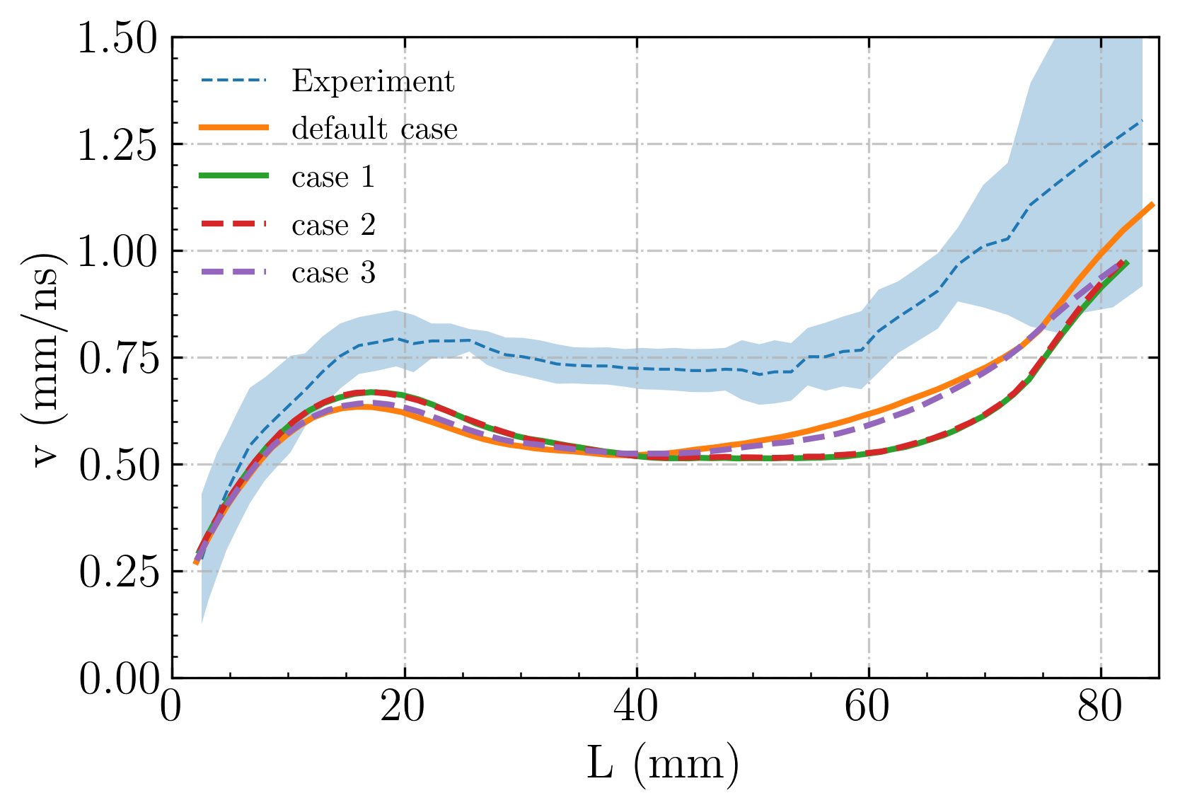
A complete description of plasma-chemical reactions for non-equilibrium discharges in nitrogen-oxygen mixtures is complex [51]. The chemical reactions considered in a fluid simulation can be as extensive as in [14], with hundreds of reactions, or as simple as in [12], considering only effective ionization rates. Nine reactions are considered as the default in this paper, including three ionization reactions, two attachment reactions and four reactions related to light emission, as shown in table 1. To make clear how important different reactions are in our discharge regime, three other cases are investigated:
- •
Case 1: reactions 1 - 3 and 6 - 9 from table 1; ionization reactions and reactions related to light emission.
- •
- •
Figure 8 shows the streamer velocity versus the streamer length for the above three cases together with the default case. The results of all cases are similar. Note in particular how the inclusion of attachment and detachment reactions hardly makes a difference. The streamer is slightly slower for case 3, in which recombination is included, but this difference is much smaller than that between the experiment and the default case. We therefore conclude that ionization reactions dominate the propagation of our discharge – a streamer of ns time scale at 0.1 bar with a background electric field of about 1.5 kV/cm. Under these conditions, attachment, detachment and recombination appear to be less important for streamer propagation.
| Reaction No. | Reaction | Reaction rate coefficient | Reference |
|---|---|---|---|
| 10 | [52] | ||
| 11 | [52] | ||
| 12 | [52] | ||
| 13 | [52] | ||
| 14 | [53] | ||
| 15 | [53] | ||
| 16 | [53] | ||
| 17 | [51] | ||
| 18 | [51] | ||
| 19 | [51] | ||
| 20 | [51] | ||
| 21 | [51] | ||
| 22 | [51] | ||
| 23 | [51] | ||
| 24 | [51] | ||
| 25 | [51] | ||
| 26 | [51] | ||
| 27 | [51] | ||
| 28 | [51] | ||
| 29 | [51] |

4.3 Transport data source
Transport coefficients for fluid models can be computed from electron-neutral cross sections using two-term or multi-term Boltzmann solvers [43, 54, 55] or Monte Carlo swarm simulations [56, 57]. For N2 and O2, there are several sets of cross section available at LXCAT [58, 59]. We here consider five such sets, namely those by Phelps [42, 46], IST Lisbon [60, 61, 62], Morgan [63], TRINITI [64] and Biagi [56, 65]. It has been common practice to normalize and adjust the total cross sections so that the transport coefficients computed with a Boltzmann solver agree well with experimentally measured swarm data with isotropic scattering. For e.g. Phelps’ cross sections, this was done with a two-term method, whereas for Biagi’s cross sections a Monte Carlo method was used. This means that even though multi-term and Monte Carlo methods are generally more accurate than two-term approaches, they do not necessarily produce transport coefficients that are closer to experimental data. In this section, we investigate how different sets of cross sections and different Boltzmann solvers affect transport coefficients and the agreement between our simulations and experiments.
We first used BOLSIG+ [43] (a two-term Boltzmann solver) to calculate transport coefficients in 80% N2 and 20% O2 for the Phelps, IST Lisbon, Morgan, TRINITI and Biagi cross sections. We used the online version BOLSIG+ via lxcat.net. Figure 9 shows how the streamer velocity in our simulations is affected by the resulting transport coefficients, which are shown in C. The streamers with the Phelps and IST Lisbon databases are fastest. With Morgan and TRINITI data, the streamers are similar to those with Phelps data up to a length of , but thereafter they behave more like those with Biagi data. The streamer with the Biagi database is the slowest, and it is about 10% slower (at the same streamer length) than the fastest one. However, regardless of the cross sections used, all simulated velocities are significantly slower than the experimental one.
To investigate the influence of the type of Boltzmann solver we also computed transport data from Biagi’s cross sections with a Monte Carlo code (available at gitlab.com/MD-CWI-NL/particle_swarm), which is similar to e.g. [57]. The resulting transport data is shown in C. With the Monte Carlo method, we computed both bulk and flux transport coefficients. Bulk coefficients describe average properties of a group of electrons, taking ionization and attachment into account, whereas flux properties are averages for ‘individual’ electrons [35, 66]. The bulk mobility is larger than the flux one at high E/N because electrons that move faster than average also typically have higher energy, and hence produce more ionization. The resulting streamer velocity with such Monte Carlo swarm flux and bulk data is shown in figure 9. It can be seen that the choice of cross sections, Boltzmann solver and flux/bulk coefficients does not significantly affect the streamer velocity, at least not sufficiently to explain the observed discrepancy with the experimental results.
To match the experimental results, artificial transport coefficients were designed based on the Phelps database by increasing the ionization coefficient and the mobility each with 20%. Figure 9 shows that with these coefficients the relative error is often below 7% when compared to the experimental velocity at the same length.

4.4 Effect of background ionization density
Positive streamers require free electrons ahead of them for their propagation, which can for example be provided by photoionization or background ionization. Under the conditions considered here (air at 0.1 bar, 50 Hz repetition frequency), we generally expect photoionization to be the dominant source of free electrons. However, background ionization could play an important role in discharge inception [36]. To investigate this, we have performed simulations with homogeneous background ionization densities of , , and m-3, in the form of electrons and positive ions. Photoionization was always included.
Note that a background ionization degree of m-3 corresponds to one electron per (10 cm)3. In reality, having so few electrons would mean that inception would be unlikely within a voltage pulse. Only electrons close to the electrode tip could start a discharge, since those farther away would quickly attach to oxygen molecules. However, in a fluid model electrons are stored as densities which can lead to unrealistic streamer inception: an electron density in the zone above breakdown can represent a fraction of an electron, but it still can grow and rapidly start a discharge. Clearly, the continuum approximation of the fluid model breaks down in these cases. We nevertheless include this unrealistic case for demonstrative purposes.
Figure 10 shows that background ionization densities in the range of to m-3 have little effect on the streamer velocity versus streamer length. With a lower background ionization degree the streamer starts a bit later, but there is no significant change in the velocity. An even higher background ionization density of m-3 (corresponding to m-3 at 1 bar) does lead to a significantly slower streamer. With this much background ionization the air surrounding the discharge has a non-negligible conductivity, reducing the field enhancement of the streamer. Since expected background ionization levels under the conditions studied here are much lower, background ionization will probably not significantly affect the streamer velocity.
The cases discussed above included spatially uniform background ionization. To study the effect of more localized initial ionization, we have also performed simulations with a Gaussian initial seed located close to the tip of the needle electrode. A neutral seed consisting of electrons and positive ions was used, given by , with m-3, the distance to the needle tip at and . Besides this initial seed, no other (uniform) initial ionization was included. The resulting streamer velocity is shown in figure 10. The streamer velocity is almost the same as for the cases with a uniform background density of up to m-3.
Remnants from previous pulses may affect the next streamer, in particular O ions from which electrons can detach. We therefore include a case with a m-3 background density of positive (N) and negative ions (O) (see Fig. 2 of [67]) and with two detachment reactions (reaction 10 and 11 from table 3). The resulting streamer velocity versus length is similar to other cases with a background density of electrons and positive ions, as shown in figure 10.
We conclude that some type of initial or background ionization is important for streamer inception, but that the stochastic nature of inception cannot be studied by a fluid model. The streamer propagation at later times is hardly affected by background ionization, at least under our conditions (air at 0.1 bar), consistent with [36, 37].

4.5 Effect of the amount of photoionization
As mentioned above, we expect photoionization to be the dominant source of free electrons ahead of the positive streamers studied here. We now investigate how the amount of photoionization affects streamer propagation. We adjust the amount of photoionization by changing the proportionality factor in equation (2). Four cases are considered: , as is used in the rest of this paper - this value is taken from [39] considering the electric field at our streamer head - and = 0.05, 0.0075 and 0.75.

Figure 11 shows the streamer velocity versus streamer length for these four cases, using a uniform background density of m-3. With ten times less photoionization, the streamer velocity increases at later times, approaching the experimental streamer velocity. This behavior, which at first seems surprising, shows the nonlinear nature of streamer discharges. Less photoionization leads to sharper electron density gradients at the streamer head, a smaller radius, and a higher degree of ionization, which can result in a higher electric field and a higher streamer velocity. However, note that there is still a qualitative discrepancy between the results of this case ( = 0.0075) and the experimental velocity in the range of 15 mm < L < 50 mm. With ten times more photoionization, the streamer is significantly slower. The electron density around the streamer head then increases sufficiently to reduce its field enhancement, as also happened in section 4.4 with a high background ionization density of . However, if the amount of photoionization is only slightly changed using (the smallest tabulated value in [39]), the streamer velocity is hardly affected, as shown in figure 11.
Additionally, we have also repeated the above simulations with an even lower background ionization density, but the results were almost identical. This indicates that even if photoionization is reduced by a factor ten, it still dominates over a background density of m-3. Finally, note that all results were obtained at a pressure of bar, at which there is less quenching than at 1 bar, see section 2.2.
4.6 Effect of gas temperature
In our experiments the lab temperature was about 293 K, but the gas temperature in the vessel was not directly measured, and we have thus far assumed it to be 300 K. The two main factors affecting the gas temperature in the vessel are heating due to repetitive discharges and cooling due to the expansion of the compressed artificial air flowing into the vessel. To investigate the effect of temperature variations, we have performed simulations with gas temperatures of 290 K, 300 K, 310 K and 360 K. The gas pressure is always 0.1 bar in the simulations. Figure 12 shows the streamer velocity for these four cases, together with the experimental result. The average streamer velocity between the two electrodes is 0.58, 0.59, 0.60 and 0.69 mm/ns for the cases at 290 K, 300 K, 310 K and 360 K, respectively. For a 10 K change in the gas temperature, the change in the streamer velocity at the same length is about 3%, on average. When the gas temperature increases 20% to 360 K, the simulated streamer velocity is closer to the experimental data, and the velocity error at the same length is less than 15%.
That a higher gas temperature leads to a higher streamer velocity is to be expected, because it leads to a higher value of in the discharge gap, just as when the applied voltage is increased. In our model, the gas number density is computed using the ideal gas law, so a reduction in gas pressure has a similar effect as an increase in temperature. However, the gas pressure was controlled to be 0.1 bar in the experiments, with an uncertainty of about 1%, so a change in pressure cannot account for the observed discrepancies.
We can roughly estimate the temperature increase caused by the repetitive discharges. From the voltage-current waveform, we estimate that about is deposited in the plasma per 200 ns pulse. At 50 Hz repetition frequency, this corresponds to W of heating power. The gas flush rate in the experiments was . Dry air at 0.1 bar and 300 K has a specific heat capacity , a density and a thermal diffusivity . If we assume heating happens uniformly and neglect losses to the vessel walls, then a rough estimate for the temperature increase would be . Alternatively, we could assume that heat is predominantly produced in the axial streamer channel and that heat diffusion occurs only in the radial direction. This results in an ‘effective’ volume of order , where is the gap size and the time. The temperature increase in this volume can then be estimated as . This is a rough estimate, not accounting for e.g., wall losses or the actual flow pattern in the vessel, nor the fact that the temperature close to the center could be considerably higher. We only have preliminary experimental data on the temperature increase, obtained with Raman scattering and optical emission spectroscopy. These measurements indicated a in the range of to , consistent with the estimate given above. We therefore conclude that gas heating might explain part of the observed differences between simulations and experiments.

4.7 Effect of applied voltage
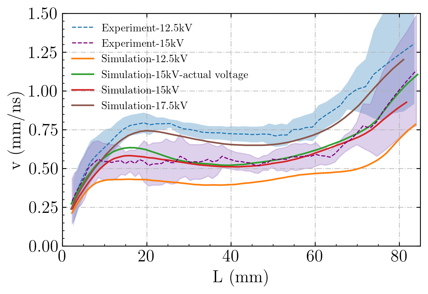
The uncertainty in the measured applied voltage is only about 2%, which is unlikely to account for the observed discrepancies in streamer velocity. However, out of scientific curiosity, we nevertheless investigate the effects of the voltage amplitude and rise time on streamer propagation below. Figure 13 shows the streamer velocity in simulations at 12.5 kV, 15 kV and 17.5 kV, together with experimental data at 12.5 kV and 15 kV. Note that for the curve labeled “Simulation-15kV-actual voltage”, the voltage is applied according to the actual waveform used in the experiment, as shown in figure 2. For the other cases, the applied voltage rises linearly from zero to the maximum voltage within 65 ns, after which it is constant. The streamer evolution is similar for the cases with an actual voltage waveform and the linearly-rising 15 kV voltage waveform, but the streamer is a little bit faster with the actual waveform, since it has a slight overshoot. In all cases, the velocity profiles follow the same pattern: the velocity first increases, then it decreases slightly, and finally it increases again as the streamers approach the opposite electrode. As expected, streamer velocities increase for higher applied voltages. The simulated streamers are always slower than the experimental ones at the same applied voltage. On average, the velocity in a simulation at 17.5 kV agrees quite well with the experimental velocity at 15 kV. However, since the experimental uncertainty in the voltage is only about 2%, this cannot explain the observed discrepancies.
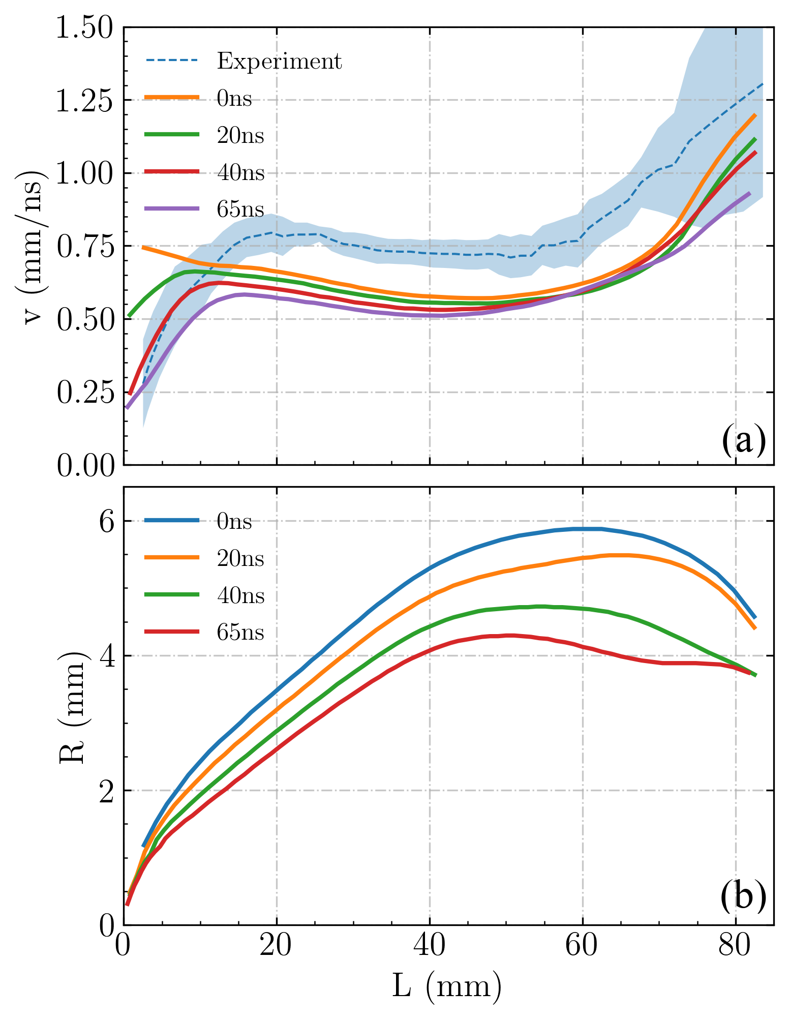
We have also studied the effect of the voltage rise time on streamer propagation, using an applied voltage of 15 kV and a variable linear voltage rise. Figure 14 shows the streamer velocity and streamer radius versus the streamer length for voltage rise times of 0, 20, 40 and 65 ns. The streamer with 0 ns rise time starts immediately when the simulation begins. Inception, here identified by a reduction in the maximal electric field, takes longer with a longer voltage rise time. With a rise time of 20 ns, 40 ns and 65 ns, the streamers incept at 10 ns, 20 ns and 30 ns, respectively. With a shorter rise time, the streamer velocity is initially higher. As the streamers get longer they propagate at the applied voltage and velocity differences become smaller when compared at the same length. Because the voltage rise time has an effect on the conductivity of the initial part of the streamer channel, small differences in velocity remain, with slightly higher velocities for shorter rise times. When comparing the velocity at the same streamer length (30 mm < L < 80 mm), the streamer velocity (averaged over length) of the 0 ns rise time case increases by about 10% compared to the 65 ns case. But there is still about a 20% discrepancy compared to the experiments. That a faster voltage rise leads to a higher streamer velocity was also found in [21]. As in [21], we also observe a larger streamer radius with a shorter voltage rise time, see figure 14 (b).
A related effect is that with a shorter voltage rise time, the electric field initially exceeds the breakdown threshold in a larger area around the needle electrode. This leads to a wider and more conductive streamer channel connected to the electrode. At later discharge stages the internal electric field in this part of the channel can therefore be lower while carrying the same electric current, which lead to less light emission around the tip of the electrode.
4.8 Finite plate electrode vs infinite plate electrode
In this paper, we apply a potential profile at the upper and lower domain boundaries to make the simulations consistent with the experimental electrode geometry, as described in section 2.2.2. This potential profile depends in particular on the radius of the HV electrode in which the needle is embedded, see figure 1. If this electrode has a small radius, then the voltage will drop more rapidly in its vicinity, leading to a background field that is higher close to the electrode and lower farther away from it. If both the grounded and HV electrodes instead have a very large radius the voltage drop will be approximately linear, and the background field homogeneous.
Here, we compare simulation results for the experimental electrode geometry with results using quasi-infinite plate electrodes and the same 10 mm long protruding needle electrode. These ‘infinite’ electrodes are incorporated by applying a voltage uniformly on the upper and lower domain boundaries. We use a linearly increasing voltage with a rise time of 65 ns for both cases. Figure 15 (a), (b) and (c) show the streamer velocity, streamer radius, and the maximal electric field at the streamer head for these two cases. The background electric field and the potential along the z axis for these two cases are shown in figure 15 (d). The use of infinite plate electrodes leads to a couple of clear differences:
- •
The voltage drop between the electrodes is now approximately linear at 0 mm < z < 85 mm, whereas with finite electrodes this drop is steeper near the HV electrode.
- •
The streamer velocity increases approximately linearly with streamer length, in contrast to the pattern of acceleration, deceleration and acceleration with finite electrodes.
- •
The streamer velocity is initially significantly lower, but when streamers have nearly bridged the whole gap their velocities are similar regardless of electrode geometry.
- •
The maximal electric field at the streamer head is now almost constant between 5 mm and 75 mm, whereas a decrease and consecutive increase are visible with finite electrodes.
- •
The background electric field is almost constant in the area 0 mm < z < 85 mm, whereas it continuously decreases from the needle electrode to the ground with finite electrodes.
- •
The streamer is thinner than with finite electrodes, and the streamer radius keeps increasing until the streamer length is about 80 mm.


4.9 Effect of boundary conditions
The experiments are performed in a quasi-cylindrical vessel with a diameter of 32.4 cm and a height of 38.0 cm. The simulation domain does not capture the whole vessel, see figure 1, so electrostatic boundary conditions for the simulation domain need to be carefully set. The upper and lower boundaries use pre-computed Dirichlet boundary conditions considering the effect of the finite plate electrodes, as described in section 2.2.2. For our default case, these values were precomputed with a FEM method for a fully axisymmetric discharge vessel with a 16 cm radius, in the absence of a discharge. However, the discharge vessel contains observation windows and gas in and outlets, so it is not fully axisymmetric, as shown in A. In particular, it contains a large window of 10 cm radius located 26 cm away from its center. Furthermore, we have thus far applied homogeneous Neumann boundary conditions for the potential at the radial boundary, whereas some type of Dirichlet boundary condition might be more appropriate. To investigate the effect of these boundary conditions for the potential, we compare our default case with three other cases:
- •
Case 1: Identical to the default case, but using the FEM solution as a Dirichlet boundary condition on the radial boundary (instead of homogeneous Neumann).
- •
Case 2: A larger 16 cm 10 cm computational domain, now using a Dirichlet zero boundary condition on the radial boundary.
- •
Case 3: Identical to case 1, but now the electric potential was pre-computed for a larger discharge vessel with a radius of 26 cm. This larger radius could account, to some extent, for the windows it contains.
Figure 16 shows the streamer velocity versus length for all cases. Case 1 and and case 2 give similar results. Compared to the default case, streamer velocities are first slightly higher, but in the range 50 mm < L < 80 mm they are lower. This implies that the use of radial Dirichlet boundary conditions reduces the potential at the streamer head at later stages. On the one hand, the agreement between case 1 and case 2 shows that our computational domain is sufficiently large for these cases, so that the discharge and boundary conditions are only weakly coupled. On the other hand, the disagreement with the default case indicates that this coupling is significantly stronger with homogeneous Neumann boundary conditions. If we instead use boundary conditions pre-computed for a larger discharge vessel (case 3), the streamer velocity is similar to the default case.
It is difficult to say which of these cases most closely matches the experiments, as the actual discharge charge vessel is not axisymmetric and contains windows. That these windows play a role was confirmed experimentally, because the streamers propagated slightly off-axis, with the deviation towards the largest window. The default case and case 3 seem to give slightly better qualitative agreement in the streamer velocity, but this could just be coincidence. However, what we can conclude is that our results are sensitive to the used electrostatic boundary conditions. For future validation studies, this could mean there is a trade-off in the size of windows for optical access: large windows facilitate measurements, but they make it harder to accurately model the electrostatic boundary conditions.
4.10 Other findings
Discharges around the edge of the HV plate electrode were observed in both the experiments and simulations. In the simulations we suppress these discharges by artificially reducing the ionization coefficient around the edge of the plate electrode to zero.
5 Summary
We have quantitatively compared simulations and experiments of single positive streamers in artificial air at . Good qualitative agreement is observed between the experimental and simulated optical emission profiles. In both cases, the streamers have similarly shaped bright heads, and darker tails. The streamer velocity and radius also show good qualitative agreement. After inception, the streamers first accelerate, then they slowly decelerate, and finally they accelerate again when approaching the grounded electrode. Quantitatively, the simulated streamer velocity is about 20% to 30% lower at the same streamer length, and the simulated radius is about 1 mm (20% to 30%) smaller. These discrepancies could be explained by a temperature increase in the experiments due to 50 Hz repetitive pulses.
Possible errors in the experimental measurements
- •
In the experiments, only preliminary measurements were available for gas temperature variations in the vessel. These indicate that the gas temperature due to previous discharges could locally rise by roughly 10 to 100 K. A temperature increase towards the upper end of this range could explain much of the observed differences between simulations and experiments.
- •
There are fluctuations in the streamer velocity obtained from the experimental images, since each image corresponds to a different discharge. The experimental velocity therefore has an intrinsic error of about 10% when compared at a particular position or time.
- •
The experimental uncertainty in the applied voltage is about 2%, and in the gas pressure it is about 1%. The observed discrepancies in streamer velocity can therefore not be explained by errors in these parameters.
Possible errors in the simulations
- •
The streamer properties in a fluid simulation depend on the used transport coefficients. The cross-section databases used here [42, 61, 56, 60] are often based on data obtained decades ago. It is difficult for us to assess the accuracy and uncertainty in this data, but more having more recent cross-section data would be helpful for the validation of simulation models.
- •
We have used a fluid model with the local field approximation. Previous studies have shown that the predictions of this model can deviate from those of particle-in-cell simulations, see e.g. [34]. However, based on recent unpublished comparisons of axisymmetric particle and fluid models in our group, we think such model error is unlikely to account for the observed discrepancies.
- •
Related to the above point, discharge inception can sometimes not accurately be modeled with a fluid model, since the continuum approximation breaks down when there are few particles. This could perhaps also account for some of the observed discrepancies.
- •
The experiments were performed with a 50 Hz repetition rate, but the simulations did not take into account remnants from previous pulses. An accumulation of long-lived excited species could for example lead to increased ionization rates. However, our simulations have been proved to be quite insensitive to initial ionization conditions.
- •
The experimental vessel contains several windows, of which one is large, and it is not fully axisymmetric. This leads to uncertainty in the boundary conditions for the electric potential in the simulations. Our simulation results are sensitive to these boundary conditions. Experimentally, an off-axis devation of the streamer towards the largest window was observed.
Summary of results for parameter studies
- 1.
The propagation of the discharge considered here – a streamer developing on ns time scale at 0.1 bar with a background electric field of about 1.5 kV/cm – is mostly controlled by ionization reactions. Attachment, detachment and recombination reactions have a much smaller effect.
- 2.
Using transport coefficients computed from different cross-section databases affects the simulated streamer evolution. However, the simulated velocities are always significantly lower than those in the experiments. The choice of Boltzmann solver (BOLSIG+ or Monte Carlo particle swarms) has little effect on the velocity. By artificially increasing both the ionization coefficient and the mobility by 20%, the simulated streamer velocity is much closer to the experimental one.
- 3.
Increasing the applied voltage increases streamer velocities. With a 17.5 kV applied voltage, the simulated streamer velocity is similar to the experimental one at 15 kV. However, the experimental uncertainty in the voltage is only about 2%. A longer voltage rise time initially slows down the streamers, but its effect is weaker at later times and longer streamer lengths.
- 4.
Initial or background ionization is essential for streamer inception, but it hardly affects streamer propagation at later times. However, a very high background ionization level leads to slower streamers, as it reduces the field enhancement at their heads.
- 5.
With ten times less photoionization, the streamer velocity increases by up to 30%, in particular when the streamer has almost bridged the gap. However, the velocity profile then differs qualitatively from the experimental measurements. With ten times more photoionization, streamers are significantly slower, as they lose some of their field enhancement due to the relatively high degree of ionization ahead of them.
- 6.
A higher gas temperature leads to higher E/N values. For a 10 K change in the gas temperature, the change in the streamer velocity at the same length is about 3%. When the gas temperature is 360 K in the simulations, the difference between the simulated and experimental streamer velocity is less than 15%.
- 7.
The size of the plate electrodes changes the background electric field in the gap. This affects the maximum electric field at the streamer head, and can lead to qualitatively different streamer propagation between the electrodes. With quasi-infinite plate electrodes, the streamer velocity monotonically increases within the gap.
Availability of model and data
The source code and documentation for the model used in this paper are available at gitlab.com/MD-CWI-NL/afivo-streamer (git commit 872d3827) and at teunissen.net/afivo_streamer. A snapshot of the code, data and experimental images is available at doi.org/10.5281/zenodo.4905873.
Acknowledgments
X.L. and S.D. were supported by STW-project 15052 “Let CO2 Spark”. X.L. was also supported by the National Natural Science Foundation of China (51777164).
We would like to thank both anonymous referees for their valuable suggestions.
PhD student contributions
X.L. performed the simulations and comparisons. S.D. built the experimental setup, performed the experiments and contributed to the data analysis.
Appendix A The discharge vessel
Figure 17 shows the geometry of the experimental discharge vessel.

Appendix B Data acquisition methods from experimental images
Here we explain how distances were determined from the experimental images, using figure 18. The size of the experimental images is 688 520 pixels. The right side of figure 18 shows the first frame in which bright emission can be observed. Assuming that light first appears around the tip of the needle electrode, the tip is located around x-pixel 538. The left side of figure 18 shows the first frame in which the streamer touches the grounded electrode. The light reflected by the flat electrode indicates that it is located around x-pixel 51. The distance between the needle electrode tip and the grounded electrode is 90 mm, so on this image 5.41 pixels correspond to 1 mm. This conversion factor is then used to determine the streamer length and radius in all the images.

Appendix C Transport coefficients value from different sources
Figure 19 gives the ionization (), attachment (), mobility () and diffusion coefficients used in section 4.3.

Appendix D Needle electrode vs initial ionized seed
In previous computational studies, an elongated ionized seed with an equal density of electrons and positive ions was often used as a pseudo-electrode to start a streamer, see e.g. [16, 47]. Due to electron drift such a seed becomes electrically screened, leading to a high electric field at its tip that can start a streamer discharge, depending on the shape and density of the seed [19]. However, to quantitatively compare simulations with experiments, we have here instead implemented an actual needle electrode in our field solver. This ensures that the electric potential at the electrode contour is equal to the applied voltage.
To compare streamers originating from a needle electrode to those originating from an ionized seed, we ran a simulation with an ionized seed of about 10 mm long with a radius of about 0.5 mm. The electron and density were m-3 at its center, with a decay at a distance above using a so-called smoothstep profile: up to , where [15]. Figure 20 (a) shows the evolution of the electric potential at the tip of the seed and the needle electrode. With an actual electrode, the potential at the needle tip agrees with the applied voltage (shown in figure 2). But with an ionized seed, the actual potential at the seed tip is lower due to the seed’s finite conductivity, and it essentially becomes part of the streamer. In other words, there is a potential drop between the plate electrode and the tip of the former seed. The streamer originating from an ionized seed is therefore slower, as shown in figure 20 (b).

References
References
- [1] Ebert U, Nijdam S, Li C, Luque A, Briels T and van Veldhuizen E 2010 Journal of Geophysical Research: Space Physics 115 ISSN 2156-2202
- [2] Laroussi M 2014 Plasma Processes and Polymers 11 1138–1141 ISSN 1612-8869
- [3] Bárdos L and Baránková H 2010 Thin Solid Films 518 6705–6713 ISSN 0040-6090
- [4] Popov N A 2016 Plasma Sources Science and Technology 25 043002 ISSN 0963-0252
- [5] Bruggeman P J, Kushner M J, Locke B R, Gardeniers J G E, Graham W G, Graves D B, Hofman-Caris R C H M, Maric D, Reid J P, Ceriani E, Rivas D F, Foster J E, Garrick S C, Gorbanev Y, Hamaguchi S, Iza F, Jablonowski H, Klimova E, Kolb J, Krcma F, Lukes P, Machala Z, Marinov I, Mariotti D, Thagard S M, Minakata D, Neyts E C, Pawlat J, Petrovic Z L, Pflieger R, Reuter S, Schram D C, Schröter S, Shiraiwa M, Tarabová B, Tsai P A, Verlet J R R, von Woedtke T, Wilson K R, Yasui K and Zvereva G 2016 Plasma Sources Science and Technology 25 053002 ISSN 0963-0252
- [6] Nijdam S, Teunissen J and Ebert U 2020 Plasma Sources Science and Technology 29 103001 ISSN 1361-6595
- [7] Babaeva N Y and Naidis G V 2021 Journal of Physics D: Applied Physics 54 223002 ISSN 0022-3727, 1361-6463
- [8] Marskar R 2020 Plasma Sources Science and Technology 29 055007 ISSN 1361-6595
- [9] Teunissen J and Ebert U 2016 Plasma Sources Science and Technology 25 044005 ISSN 0963-0252, 1361-6595
- [10] Plewa J M, Eichwald O, Ducasse O, Dessante P, Jacobs C, Renon N and Yousfi M 2018 Journal of Physics D: Applied Physics 51 095206 ISSN 0022-3727
- [11] Roache P J 1998 Verification and Validation in Computational Science and Engineering 0th ed (Albuquerque, N.M: Hermosa Pub) ISBN 978-0-913478-08-0
- [12] Bagheri B, Teunissen J, Ebert U, Becker M M, Chen S, Ducasse O, Eichwald O, Loffhagen D, Luque A, Mihailova D, Plewa J M, van Dijk J and Yousfi M 2018 Plasma Sources Science and Technology 27 095002 ISSN 1361-6595
- [13] Pancheshnyi S, Nudnova M and Starikovskii A 2005 Physical Review E 71 ISSN 1539-3755, 1550-2376
- [14] Ono R and Komuro A 2020 Journal of Physics D: Applied Physics 53 035202 ISSN 0022-3727, 1361-6463
- [15] Teunissen J and Ebert U 2017 Journal of Physics D: Applied Physics 50 474001 ISSN 0022-3727, 1361-6463
- [16] Bagheri B, Teunissen J and Ebert U 2020 Plasma Sources Science and Technology 29 125021 ISSN 0963-0252, 1361-6595
- [17] Francisco H, Bagheri B and Ebert U 2021 Plasma Sources Science and Technology ISSN 0963-0252
- [18] Briels T M P, Kos J, Winands G J J, van Veldhuizen E M and Ebert U 2008 Journal of Physics D: Applied Physics 41 234004 ISSN 0022-3727, 1361-6463
- [19] Luque A, Ratushnaya V and Ebert U 2008 Journal of Physics D: Applied Physics 41 234005 ISSN 0022-3727, 1361-6463
- [20] Komuro A, Ono R and Oda T 2012 Journal of Physics D: Applied Physics 45 265201 ISSN 0022-3727, 1361-6463
- [21] Komuro A, Ono R and Oda T 2013 Plasma Sources Science and Technology 22 045002 ISSN 1361-6595 URL http://dx.doi.org/10.1088/0963-0252/22/4/045002
- [22] Komuro A, Matsuyuki S and Ando A 2018 Journal of Physics D: Applied Physics 51 445204 ISSN 0022-3727, 1361-6463
- [23] Eichwald O, Ducasse O, Dubois D, Abahazem A, Merbahi N, Benhenni M and Yousfi M 2008 Journal of Physics D: Applied Physics 41 234002 ISSN 0022-3727
- [24] Nijdam S, Teunissen J, Takahashi E and Ebert U 2016 Plasma Sources Science and Technology 25 044001 ISSN 0963-0252, 1361-6595
- [25] Marode E, Dessante P and Tardiveau P 2016 Plasma Sources Science and Technology 25 064004 ISSN 1361-6595
- [26] Brisset A, Gazeli K, Magne L, Pasquiers S, Jeanney P, Marode E and Tardiveau P 2019 Plasma Sources Science and Technology 28 055016 ISSN 1361-6595
- [27] Zhu Y, Chen X, Wu Y, Hao J, Ma X, Lu P and Tardiveau P 2021 Plasma Sources Science and Technology ISSN 0963-0252
- [28] Tholin F, Rusterholtz D L, Lacoste D A, Pai D Z, Celestin S, Jarrige J, Stancu G D, Bourdon A and Laux C O 2011 IEEE Transactions on Plasma Science 39 2254–2255 ISSN 1939-9375
- [29] Pechereau F, Le Delliou P, Jánský J, Tardiveau P, Pasquiers S and Bourdon A 2014 IEEE Transactions on Plasma Science 42 2346–2347 ISSN 1939-9375
- [30] Yousfi M, Eichwald O, Merbahi N and Jomaa N 2012 Plasma Sources Science and Technology 21 045003 ISSN 0963-0252
- [31] Hofmans M, Viegas P, Rooij O v, Klarenaar B, Guaitella O, Bourdon A and Sobota A 2020 Plasma Sources Science and Technology 29 034003 ISSN 0963-0252 publisher: IOP Publishing URL https://doi.org/10.1088/1361-6595/ab6d49
- [32] Viegas P, Hofmans M, van Rooij O, Obrusník A, L M Klarenaar B, Bonaventura Z, Guaitella O, Sobota A and Bourdon A 2020 Plasma Sources Science and Technology 29 095011 ISSN 1361-6595 URL http://dx.doi.org/10.1088/1361-6595/aba7ec
- [33] Li C, Teunissen J, Nool M, Hundsdorfer W and Ebert U 2012 Plasma Sources Sci. Technol. 15
- [34] Markosyan A H, Teunissen J, Dujko S and Ebert U 2015 Plasma Sources Science and Technology 24 065002 ISSN 0963-0252, 1361-6595
- [35] Dujko S, Markosyan A H, White R D and Ebert U 2013 Journal of Physics D: Applied Physics 46 475202 ISSN 0022-3727, 1361-6463
- [36] Nijdam S, Wormeester G, van Veldhuizen E M and Ebert U 2011 Journal of Physics D: Applied Physics 44 455201 ISSN 0022-3727, 1361-6463
- [37] Nijdam S, Takahashi E, Markosyan A H and Ebert U 2014 Plasma Sources Science and Technology 23 025008 ISSN 0963-0252, 1361-6595
- [38] Teunissen J and Ebert U 2018 Computer Physics Communications 233 156–166 ISSN 00104655
- [39] Zheleznyak M, Mnatsakanyan A and Sizykh S 1982 High Temperature 20 357–362 ISSN 0018-151X
- [40] Bourdon A, Pasko V P, Liu N Y, Célestin S, Ségur P and Marode E 2007 Plasma Sources Science and Technology 16 656–678 ISSN 0963-0252, 1361-6595
- [41] Bagheri B and Teunissen J 2019 Plasma Sources Science and Technology 28 045013 ISSN 1361-6595
- [42] Phelps A V and Pitchford L C 1985 Physical Review A 31 2932–2949 ISSN 0556-2791
- [43] Hagelaar G J M and Pitchford L C 2005 Plasma Sources Science and Technology 14 722–733 ISSN 0963-0252, 1361-6595
- [44] Pancheshnyi S V, Sobakin S V, Starikovskaya S M and Starikovskii A Y 2000 Plasma Physics Reports 26 1054–1065 ISSN 1562-6938
- [45] BOLSIG+ solver ver. 03/2016 www.lxcat.net
- [46] Phelps database (N2,O2) www.lxcat.net, retrieved on January 19, 2021
- [47] Li X, Sun A, Zhang G and Teunissen J 2020 Plasma Sources Science and Technology 29 065004 ISSN 0963-0252
- [48] Hansen E W and Law P L 1985 Journal of the Optical Society of America A 2 510 ISSN 1084-7529, 1520-8532
- [49] Schafer R 2011 IEEE Signal Processing Magazine 28 111–117 ISSN 1053-5888
- [50] Naidis G V 2009 Physical Review E 79 ISSN 1539-3755, 1550-2376
- [51] Kossyi I A, Kostinsky A Y, Matveyev A A and Silakov V P 1992 Plasma Sources Science and Technology 1 207–220 ISSN 0963-0252, 1361-6595
- [52] Pancheshnyi S 2013 Journal of Physics D: Applied Physics 46 155201 ISSN 0022-3727
- [53] Aleksandrov N L and Bazelyan E M 1999 Plasma Sources Science and Technology 8 285–294 ISSN 0963-0252
- [54] Stephens J 2018 Journal of Physics D: Applied Physics 51 125203 ISSN 0022-3727
- [55] Tejero-del-Caz A, Guerra V, Gonçalves D, da Silva M L, Marques L, Pinhão N, Pintassilgo C D and Alves L L 2019 Plasma Sources Science and Technology 28 043001 ISSN 0963-0252
- [56] Biagi S F 1999 Nuclear Instruments and Methods in Physics Research Section A: Accelerators, Spectrometers, Detectors and Associated Equipment 421 234–240 ISSN 0168-9002
- [57] Rabie M and Franck C M 2016 Computer Physics Communications 203 268–277 ISSN 0010-4655
- [58] Pancheshnyi S, Biagi S, Bordage M, Hagelaar G, Morgan W, Phelps A and Pitchford L 2012 Chemical Physics 398 148–153 ISSN 03010104
- [59] Carbone E, Graef W, Hagelaar G, Boer D, Hopkins M M, Stephens J C, Yee B T, Pancheshnyi S, van Dijk J and Pitchford L 2021 Atoms 9 16 number: 1 Publisher: Multidisciplinary Digital Publishing Institute URL https://www.mdpi.com/2218-2004/9/1/16
- [60] Alves L L 2014 Journal of Physics: Conference Series 565 012007 ISSN 1742-6596 publisher: IOP Publishing URL https://doi.org/10.1088/1742-6596/565/1/012007
- [61] Loureiro J and Ferreira C M 1986 Journal of Physics D: Applied Physics 19 17–35 ISSN 0022-3727
- [62] Ist lisbon database (N2,O2) www.lxcat.net, retrieved on January 19, 2021
- [63] Morgan database (N2,O2) www.lxcat.net, retrieved on January 19, 2021
- [64] Triniti database (N2,O2) www.lxcat.net, retrieved on January 19, 2021
- [65] Biagi database (N2,O2) www.lxcat.net, retrieved on January 19, 2021
- [66] Petrović Z L, Dujko S, Marić D, Malović G, Nikitović Ž, Šašić O, Jovanović J, Stojanović V and Radmilović-Ra\djenović M 2009 Journal of Physics D: Applied Physics 42 194002 ISSN 0022-3727
- [67] Pancheshnyi S 2005 Plasma Sources Science and Technology 14 645–653 ISSN 0963-0252, 1361-6595