Markov Localisation using Heatmap Regression and Deep Convolutional Odometry

Markov localisation, shown by the gray dotted line on fig. 1, operates by taking the state-space of the autonomous agent, given by $\prescript{}{\hskip 0.7113pt}{\mathbf{p}}_{t}\in\prescript{}{\hskip 0.7113pt}{\mathbb{{P}}}_{t}$ and discretising it into in a grid defined as

where each $\prescript{}{\hskip 0.7113pt}{\mathbf{\dot{x}}}_{t}^{k}$ is a cell in the grid $\prescript{}{\hskip 0.7113pt}{\mathbb{{\dot{X}}}}_{t}$ at time $t$. The grid $\prescript{}{\hskip 0.7113pt}{\mathbb{{\dot{X}}}}_{t}$ spans all possible states in the state-space $\prescript{}{\hskip 0.7113pt}{\mathbb{{P}}}_{t}$. For a ground-based vehicle, it is sufficient to represent the state space of the vehicle as a 3-dof vector $\prescript{}{\hskip 0.7113pt}{\mathbf{\dot{x}}}=\left\langle x,y,\theta\right\rangle$. This means that the discretised grid $\prescript{}{\hskip 0.7113pt}{\mathbb{{\dot{X}}}}_{t}$ is a 3 dimensional volume. This volume consists of $\left\langle x,y\right\rangle$ planes and $\theta$ slices. More explicitly, this volume consists of a tensor of size $[\Theta\times X\times Y]$, where each cell represents the likelihood that the robot’s position lies within that cell’s bounds. Under a Markov assumption, this likelihood can be defined as

which implies that the pose likelihood is conditioned on the sensor observations $\prescript{}{\hskip 0.7113pt}{z}_{t}\in\prescript{}{\hskip 0.7113pt}{\mathbb{{Z}}}_{t}$ and the odometry measurements $\prescript{}{\hskip 0.7113pt}{u}_{t}\in\prescript{}{\hskip 0.7113pt}{\mathbb{{U}}}_{t}$ and is fully described by the sensor model

the motion model

and the prior likelihood of the pose

which implies this measurement can be performed iteratively. In this work, we use a heatmap regression sensor model (III-B) to update the $[X\times Y]$ volume, while using convolutional odometry (III-C) for the orientation. We additionally perform a likelihood-volume-to-pose extraction, which consists of fitting a Gaussian distribution to the likelihood volume and reporting the mean.

One of the main reasons grid-based localisation was widely considered intractable was because the sensor model (equation 3) has to be estimated for every cell in the grid. Estimating this likelihood for sensors such as lidar, sonar or even RGB-D cameras can involve expensive ray-casting for each beam. This presents a practical issue when there are large areas of the grid that we are almost certain not to be the correct location. Instead, we propose to use a fcn (fcn) trained for pose regression to replace the sensor model.

Using an fcn has several important advantages. Firstly, it allows a sensor model to be trained for any arbitrary sensor without the need for explicit mathematical derivation (although requiring training data). Secondly, the likelihood for every cell can be estimated simultaneously.

The sensor model introduced in the previous section does not measure the likelihood of the agent’s orientation $\theta$. Instead, we use a novel convolution-based odometry layer as a motion model which estimates $\theta$. Our model is efficient, so there is no need to artificially limit the update rate other than to guarantee at least one cell of displacement. This means that, assuming a non-holonomic agent, the motion model can propagate pose likelihoods in a manner that also selects the correct orientation.

Markov localisation relies on a motion model (equation 4) to propagate likelihoods into the correct areas of the grid. Normally, this is implemented as a shift according to the odometry measurement, followed by diffusion using convolution with a separable Gaussian. The kernel of this Gaussian is computed based on the odometry’s uncertainty. For a 3-dof likelihood grid this is a relatively expensive operation as it would require a set of 3 shifts, and a 3D convolution which would be prohibitively expensive on a CPU. However, we formulate the odometry kernel as a deep learning layer that enables us to perform an efficient operation on the GPU by mapping the 3 shifts and 3 convolutions into a singe 2D convolution kernel. By building our sensor and motion model as custom layers on a cnn, the entire framework can operate in a single forward pass on one GPU incredibly quickly. In order to estimate our odometry kernel for 2D convolution, we first look at how the odometry maps into a simple 3D convolution kernel. The odometry data from any non-holonomic 3-dof vehicle can be decomposed as

where $\prescript{}{\hskip 0.7113pt}{\delta\theta}_{t}^{1}$ is a rotation followed by a forward translation $\prescript{}{\hskip 0.7113pt}{\delta x}_{t}$ and a final rotation $\prescript{}{\hskip 0.7113pt}{\delta\theta}_{t}^{2}$ [22]. Gaussian noise can be applied to each component independently, producing a new set of odometry estimates $\prescript{}{\hskip 0.7113pt}{\hat{\delta}\theta}_{t}^{1},\prescript{}{\hskip 0.7113pt}{\hat{\delta}x}_{t},\prescript{}{\hskip 0.7113pt}{\hat{\delta}\theta}_{t}^{2}$.

In order to map this into a 3D kernel, we take this representation and map it into a vector as

However, this odometry is not directly applicable to every $\theta_{c}\in\Theta$ channel in our likelihood volume. In order to apply the odometry, we align it such that “forward” motion represents the orientation of the $\theta_{c}$ bin. This is done using a simple 2D rotation matrix defined as

for every $\theta_{c}$ in the likelihood volume. Each of these matrices can then be multiplied with the linear component of the odometry vector

in order to obtain a set of rotated odometries for each channel.

The set of rotated odometries are directly mapped into a kernel for convolution. However, it is first necessary map these odometries to the resolution of the likelihood grid, which can be done as $\prescript{}{\hskip 0.7113pt}{\mathbb{{S}}}_{t}^{\prime}=\prescript{}{\hskip 0.7113pt}{\mathbb{{S}}}_{t}\odot\prescript{}{\hskip 0.7113pt}{\mathbf{\lambda}}$ where $\odot$ is element wise multiplication and $\prescript{}{\hskip 0.7113pt}{\mathbf{\lambda}}=\left\langle\frac{1}{r_{x}},\frac{1}{r_{y}},\frac{1}{r_{\theta}}\right\rangle$ is the resolution of the grid which has been tiled $\Theta$ times.

We are not guaranteed that the odometry will be larger than a single cell in the likelihood grid. For this reason, it is necessary to accumulate odometry measurements over time as

where $\prescript{}{\hskip 0.7113pt}{\mathbb{{T}}}_{t}^{\prime}=\prescript{}{\hskip 0.7113pt}{\mathbb{{T}}}_{t}-\lfloor\prescript{}{\hskip 0.7113pt}{\mathbb{{T}}}_{t}\rfloor$ and $\lfloor\prescript{}{\hskip 0.7113pt}{\mathbb{{T}}}_{t}\rfloor$ is the odometry applied to the likelihood volume $\prescript{}{\hskip 0.7113pt}{\mathbb{{\dot{X}}}}_{t}$.

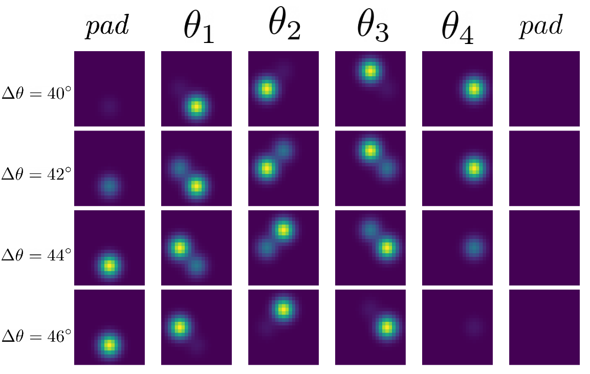
Applying $\lfloor\prescript{}{\hskip 0.7113pt}{\mathbb{{T}}}_{t}\rfloor$ to $\prescript{}{\hskip 0.7113pt}{\mathbb{{\dot{X}}}}_{t}$ can be done by converting the rotated odometries into a series of 3D kernels for 2D convolution. The first step is to map each vector $\prescript{}{\hskip 0.7113pt}{\mathbf{\tau}}_{t}\in\lfloor\prescript{}{\hskip 0.7113pt}{\mathbb{{T}}}_{t}\rfloor$ into a 3D kernel. To do this we take every element of $\prescript{}{\hskip 0.7113pt}{\mathbf{\tau}}_{t}$ and convert it into a discrete 1D Gaussian kernel of size $\left\langle k_{\theta},k_{x},k_{y}\right\rangle$. These kernels are then combined linearly to produce a 3D kernel $\prescript{}{\hskip 0.7113pt}{\mathbf{K}}_{c}$ of size $\left\langle K_{\theta},K_{x},K_{y}\right\rangle$. This allows us to perform a 2D convolution on a subset of the likelihood grid for each 3D kernel. This subset consists of the channel the kernel was estimated for as well as the $K_{\theta}$ channels around it. In order to perform the operation as a single pass of a 2D convolution on GPU hardware, we stack these kernels into a single kernel. Each 3D kernel is offset so that it is centered on the $\theta_{c}$ channel it corresponds to, giving us a kernel with $\theta_{c}$ Gaussian distributions. Fig. 3 shows a visualisation of the odometry kernel when $\Theta=4$ for a simple forward motion. Each column represents a $\theta_{c}$ channel (along with padding), while each row represents the rotated odometry for each angle bin. Notice how each $\theta_{c}$ channel represents the forward motion differently. Similarly, as the rows go down, the likelihoods shift between the different theta channels and respect the circular nature of $\theta$ by looping from the last bin to the first.

While it may seem like these are an expensive set of convolutions, it is important to remember that these are all performed directly on the GPU. More importantly, our Markov localisation approach is entirely GPU bound. Both our sensor and motion model are computed directly on the GPU with no need to ever retrieving the cost volume. This makes our approach both quick and efficient. In the following section, we will show that not only is our approach fast but it is also capable of producing state-of-the-art results for localisation.

The dataset consists of 6 sequences of images captured at different landmarks across the city of Cambridge (UK) using a hand-held camera. Each sequence consists of anywhere between $300$ and $6000$ images which are then split between train and test sets. Ground-truth poses are estimated using sfm (sfm) [5] software. The sensor experiences 6-dof motion during capture. Furthermore the sfm software does not guarantee that there is a well-defined ground plane. This makes the dataset inherently difficult for our approach, as we only localise in a 3-dof space. Since most of the motion of the sensor is planar, we overcome this limitation by using an svd (svd) to regress a dominant plane and therefore the height of the sensor.

Table I shows a comparison against several pose-regression networks. We show the median pose error on all 3 spatial axis, as reported in [12]. It is important to note that this is an unfavourable scenario for our 3-dof localisation, as our network does not directly regress the height of the sensor. We also do not estimate the orientation of the sensor, as the heatmap regressor should be able to cope with the appearance variation. Regardless, our heatmap regressor is able to outperform several state-of-the-art regression methods in 4 out of 6 scenarios. We believe there are several reasons for this. Firstly, a heatmap-based loss provides a more uniform supervision signal than a pose-based loss, as the heatmaps do not scale with the magnitude of the pose space. Secondly, and most importantly, while we do not strictly enforce multi-modal distributions with our losses, the network is capable of modelling them. This allows the network to predict uncertain poses without incurring a penalty. In the KingsCollege scenario, we are only outperformed by PoseNet Geometric [12], which makes use of an additional source of supervision: the 3D reconstruction points of the ground truth. For the OldHospital scenario, we are outperformed by Walch et al. [24] most likely because the self-repeating nature of the architecture is well-suited to the spatial LSTMs they employ.

One of the main advantages of our approach is the ability to generalise to self-similar environments. Car-parks are interesting environments for localisation, as they tend to be self-similar within each floor as well as across multiple floors. By their nature, accurate localisation within a multi-storey car-park requires a multi-modal distribution.

References

- [1] Samarth Brahmbhatt, Jinwei Gu, Kihwan Kim, James Hays, and Jan Kautz. Geometry-aware learning of maps for camera localization. In IEEE/CVF Conference on Computer Vision and Pattern Recognition (CVPR), pages 2616–2625, 2018.
- [2] Wolfram Burgard, Armin B Cremers, Dieter Fox, Dirk Hähnel, Gerhard Lakemeyer, Dirk Schulz, Walter Steiner, and Sebastian Thrun. Experiences with an interactive museum tour-guide robot. Artificial intelligence, 114(1-2):3–55, 1999.
- [3] Wolfram Burgard, Dieter Fox, Daniel Hennig, and Timo Schmidt. Estimating the absolute position of a mobile robot using position probability grids. In National Conference on Artificial Intelligence, pages 896–901, 1996.
- [4] Tim Caselitz, Bastian Steder, Michael Ruhnke, and Wolfram Burgard. Monocular camera localization in 3D LiDAR maps. In International Conference on Intelligent Robots and Systems (IROS), pages 1926–1931. IEEE/RSJ, 2016.
- [5] Wu Changchang. Towards Linear-Time Incremental Structure from Motion. In International Conference on 3D Vision (3DV), pages 127–134, 2013.
- [6] Hang Chu, Dong Ki Kim, and Tsuhan Chen. You are here: Mimicking the Human Thinking Process in Reading Floor-Plans. In International Conference on Computer Vision (ICCV), pages 2210–2218, 2015.
- [7] Frank Dellaert, Dieter Fox, Wolfram Burgard, and Sebastian Thrun. Monte Carlo localization for mobile robots. In International Conference on Robotics and Automation (ICRA), number May, pages 1322–1328, Detroit, 1999. IEEE.
- [8] Dieter Fox, Wolfram Burgard, Frank Dellaert, and Sebastian Thrun. Monte Carlo Localization: Efficient Position Estimation for Mobile Robots. In Association for the Advancement of Artificial Intelligence (AAAI), pages 343–349, 1999.
- [9] Kaiming He, Xiangyu Zhang, Shaoqing Ren, and Jian Sun. Deep residual learning for image recognition. In IEEE/CVF Conference on Computer Vision and Pattern Recognition (CVPR), pages 770–778, 2016.
- [10] Joao F Henriques and Andrea Vedaldi. Mapnet: An allocentric spatial memory for mapping environments. In IEEE/CVF Conference on Computer Vision and Pattern Recognition (CVPR), pages 8476–8484, 2018.
- [11] Alex Kendall and Roberto Cipolla. Modelling uncertainty in deep learning for camera relocalization. In IEEE International Conference on Robotics and Automation (ICRA), pages 4762–4769. IEEE, 2016.
- [12] Alex Kendall and Roberto Cipolla. Geometric loss functions for camera pose regression with deep learning. In IEEE/CVF Conference on Computer Vision and Pattern Recognition (CVPR), pages 5974–5983, 2017.
- [13] Alex Kendall, Matthew Grimes, and Roberto Cipolla. Posenet: A convolutional network for real-time 6-dof camera relocalization. In IEEE/CVF Conference on Computer Vision and Pattern Recognition (CVPR), pages 2938–2946, 2015.
- [14] Jong-Hwan Lim and Chul-Ung Kang. Grid-based localization of a mobile robot using sonar sensors. Korean Society of Mechanical Engineers (KSME) International Journal, 16(3):302–309, 2002.
- [15] Oscar Mendez, Simon Hadfield, Nicolas Pugeault, and Richard Bowden. SeDAR - Semantic Detection and Ranging: Humans can localise without LiDAR, can robots? In International Conference on Robotics and Automation (ICRA), Brisbane, Australia, 2018. IEEE.
- [16] Tayyab Naseer and Wolfram Burgard. Deep regression for monocular camera-based 6-dof global localization in outdoor environments. In IEEE/RSJ International Conference on Intelligent Robots and Systems (IROS), pages 1525–1530. IEEE, 2017.
- [17] Peer Neubert, Stefan Schubert, and Peter Protzel. Sampling-based Methods for Visual Navigation in 3D Maps by Synthesizing Depth Images. In International Conference on Intelligent Robots and Systems (IROS), 2017.
- [18] Johannes Poschmann, Peer Neubert, Stefan Schubert, and Peter Protzel. Synthesized Semantic Views for Mobile Robot Localization. In European Conference on Mobile Robotics (ECMR), pages 403–408, Paris, 2017. IEEE.
- [19] Torsten Sattler, Qunjie Zhou, Marc Pollefeys, and Laura Leal-Taixe. Understanding the limitations of cnn-based absolute camera pose regression. In IEEE/CVF Conference on Computer Vision and Pattern Recognition (CVPR), pages 3302–3312, 2019.
- [20] Reid Simmons and Sven Koenig. Probabilistic robot navigation in partially observable environments. In International Joint Conference on Artificial Intelligence (IJCAI), volume 95, pages 1080–1087, 1995.
- [21] Jurgen Sturm, Nikolas Engelhard, Felix Endres, Wolfram Burgard, and Daniel Cremers. A benchmark for the evaluation of RGB-D SLAM systems. In International Conference on Intelligent Robots and Systems (IROS), pages 573–580. IEEE/RSJ, 2012.
- [22] Sebastian Thrun, Wolfram Burgard, and Dieter Fox. Robot Motion. In Probabilistic Robotics, chapter 5, pages 135–136. MIT Press, Cambridge, Massachussets, 2006.
- [23] Sebastian Thrun, Wolfram Burgard, and Dieter Fox. TheEKFLocalizationAlgorithm. In Probabilistic Robotics, chapter 4.5.2, pages 96–113. MIT Press, Cambridge, Massachussets, 2006.
- [24] Florian Walch, Caner Hazirbas, Laura Leal-Taixé, Torsten Sattler, Sebastian Hilsenbeck, and Daniel Cremers. Image-based localization using lstms for structured feature correlation. In International Conference on Computer Vision (ICCV), October 2017.
- [25] Nan Yang, Lukas von Stumberg, Rui Wang, and Daniel Cremers. D3vo: Deep depth, deep pose and deep uncertainty for monocular visual odometry. In IEEE/CVF Conference on Computer Vision and Pattern Recognition (CVPR), pages 1281–1292, 2020.