Spectral theory of weighted hypergraphs via tensors
Abstract
One way to study a hypergraph is to attach to it a tensor. Tensors are a generalization of matrices, and they are an efficient way to encode information in a compact form. In this paper we study how properties of weighted hypergraphs are reflected on eigenvalues and eigenvectors of their associated tensors. We also show how to efficiently compute eingenvalues with some techniques from numerical algebraic geometry.
Keywords: Spectral hypergraph theory, Tensors, Weighted hypergraphs, Eigenvalues
1 Introduction
Spectral hypergraph theory
Spectral graph theory is the study of the qualitative properties of a graph that can be inferred from the spectrum, i.e. the multiset of the eigenvalues, of a square matrix associated to . If the vertices of are labelled as , the considered square matrices are usually the adjacency matrix , whose entries are
the Kirchhoff Laplacian
where is the diagonal matrix of the degrees, and the normalized Laplacian
where is the identity matrix. There is a correspondence between graphs and each of these operators. While there exist non-isomorphic graphs with the same spectra, nevertheless such spectra are known to detect many important geometric properties of the graph. Thus, if two graphs are isospectral with respect to a given operator, they have similar structures. Spectral graph theory has a long history, it has many connections with the spectral theory in Riemannian geometry, and it is widely used in applications. In fact, because empirical networks can often be modeled as graphs, the computation of the spectra is a valuable tool for studying and analyzing real data. Moreover, this theory also finds applications in the study of dynamical systems on graphs. The normalized Laplacian is isospectral to the random walk Laplacian
whose off-diagonal entry
is minus the probability that a random walker goes from to . Hence, the spectral theory of and has many connections with random walks on graphs. We refer the reader to [8, 7] for classical monographs on the spectral theory of graphs.
Hypergraphs are defined as a generalization of graphs in which edges can link more than two vertices, that is, edges are sets of vertices of any cardinality. They allow the modeling of many more real networks than graphs, therefore they are often used in applications as well, see for instance [4, 5, 16, 29, 36, 17]. It is natural to ask what is the best way to generalize spectral graph theory to the case of hypergraphs, but the answer is not univocal. In fact, the spectral theory of hypergraphs can be studied either via matrices or via tensors, and the two approaches have different advantages. While there is a correspondence between hypergraphs and their associated tensors, the same does not hold for the hypergraph adjacency and Laplacian matrices. Hence, the spectrum of a hypergraph tensor is expected to detect more precise structural properties of the hypergraph than the spectrum of a hypergraph matrix. However, the tensor eigenvalue problem is NP-hard [11], therefore it is more convenient to consider matrices for the analysis of big data that are modeled with hypergraphs.
In this work, we bring forward the spectral theory of hypergraphs via tensors and we generalize the operators in [2, 3, 24, 25, 1, 9] to the case of weighted hypergraphs, for which each edge has a positive weight. We show that most of the spectral properties that are known for unweighted hypergraphs can be generalized to the weighted case, and we prove several results which are also new for the unweighted case. We refer to [27] for a monograph on the spectral theory via tensors of uniform, unweighted hypergraphs. We refer to [15] for the related spectral theory of multilayer networks. For completeness, we also refer the reader to [22, 30, 31, 23, 13, 14, 32] for a vast — but by no means complete — literature on the spectral theory of hypergraphs via matrices.
Tensors
We start by recalling several definitions and properties of tensors that will be needed throughout the paper. We refer to [27] for a monograph on this topic. Given ,
we denote by the set . We indicate a vector in by . We write if for every .
Let . A -th order -dimensional tensor consists of complex entries
where . The tensor is symmetric if its entries are invariant under any permutation of their indices.
One of the many differences between the spectral theory of matrices and of tensors is that a the eigenvalues of a real symmetric tensor do not need to be real.
Given a vector , define by
Let be the vector with entries . If for some and some non-zero vector , then we say that is an eigenpair for . The number is an eigenvalue of and is an eigenvector. The spectral radius of , denoted , is the largest modulus of the eigenvalues of .
Let denote the -th order -th dimensional unit tensor, with entries
Just as matrices, tensors have a determinant. As illustrated in [27, Section 2.1.3], the determinant of a tensor is the resultant of the system of equations . It is a polynomial in the entries of that vanishes if and only if the system has a non-zero solution. As shown in [27, Theorem 2.12], the eigenvalues of are the roots of the characteristic polynomial
of . The spectrum of , denoted , is the multiset of its eigenvalues, counted with multiplicity as roots of the characteristic polynomial. An eigenpair is given by an -eigenvalue and an -eigenvector, respectively, if and . We let denote the set of distinct -eigenvalues of .
The tensor is non-negative if all its entries are non-negative. The tensor is weakly irreducible if, for any non-empty proper index subset of , there is at least one entry
where and at least one index , for .
Similarly, is reducible if there exists a non-empty proper set of such that
for each , . It is irreducible if it is not reducible.
In [27, Theorems 3.25 and 3.26], the Perron-Frobenius theorem for non-negative matrices has been generalized to weakly irreducible non-negative tensors.
Theorem 1.1.
If is non-negative and weakly irreducible, then
is a positive -eigenvalue, with a positive -eigenvector . Furthermore, is the unique -eigenvalue of with a positive -eigenvector, and is the unique positive -eigenvector associated to , up to a multiplicative constant.
Now, is diagonally dominated if, for each ,
| (1) |
By [28, Theorem 2], if is any tensor and is an eigenvalue for , then there exists such that
| (2) |
An immediate consequence is the following
Corollary 1.2.
If is a diagonally dominated tensor, then all its -eigenvalues are non-negative.
Eigenvalue multiplicities
For a given tensor, the algebraic multiplicity of an eigenvalue , denoted , is its multiplicity as a root of the characteristic polynomial. The geometric multiplicity of , denoted , is the dimension of its eigenvariety, i.e. the variety of its eigenvectors. While algebraic and geometric multiplicity coincide for symmetric matrices, this is not always the case for symmetric tensors. In [12, Conjecture 1.1], it is conjectured that, for any ,
Given an eigenvalue , we also introduce its span multiplicity, denoted , as the dimension of the vector space
Clearly, . In [26, Section 3] it is conjectured that, for any ,
If is a real eigenvalue, we introduce its Hspan multiplicity, denoted , as the dimension of the vector space
In the case of symmetric matrices, every eigenvalue is an -eigenvalue and
In spectral graph theory and spectral hypergraph theory via matrices, the multiplicity of an eigenvalue is often studied by counting the maximum number of its linearly independent eigenvectors. This is what motivates us to study the span and the Hspan multiplicities.
Stirling numbers
Given a multiset , let be the set obtained from by not accounting for multiplicity. Given a -th order -dimensional tensor and an index set of cardinality , we say that an entry of corresponds to if . We let
Given , we define its -th row as the -order -dimensional tensor obtained by setting the first index of equal to . We also set
Observe that it does not depend on . As shown in [24],
from which it follows that
By Proposition 5.5 in [21], we can write , where
is the Stirling number of the second kind. This can be seen from the fact that counts the number of -partitions of a set of cardinality , while counts the number of permutations of objects. Hence,
In particular, . The above characterization of allows us to give a description of the hypergraph tensors which is simpler than the one in [2, 3, 24, 25, 1].
Weighted hypergraphs
Throughout the paper, we fix a weighted hypergraph with vertex set , edge set and weight function . We assume that each edge contains at least two vertices.
Given , its degree is
Given , we denote its cardinality by . We let
is -regular if for each ; it is -uniform if for each .
Given , we let
is connected if, for every pair of vertices , there exists a path that connects and , i.e. there exist and such that , , and for each .
The hypergraph is unweighted if for each . In this case, we use the notation .
A simple graph is an unweighted -uniform hypergraph.
Structure of the paper
In Section 2 we introduce the tensors we are interested in. Our definitions generalize the known hypergraph tensors to the case of weighted hypergraphs. In Section 3 we prove some basic properties of the eigenvalues of such tensors. Section 4 is devoted to duplicate vertices, a combinatorial feature of a hypergraph that has a clear impact on the spectra. This is particularly evident for hyperflowers, a remarkable family of hypergraphs that generalize star graphs and that we analyse in Section 5. Section 6 adds more words to our dictionary. We are able to translate properties of the hypergraphs, such as being bipartite or colorable, to spectral symmetries. Finally, in Section 7 we show how to effectively compute eigenvalues and their geometric multiplicities. We apply techniques from numerical algebraic geometry.
2 Hypergraph tensors
As we recalled in the introduction, there are several tensors attached to a hypergraph. In this section we generalize these tensors for weighted hypergraphs.
Let be a weighted hypergraph on nodes, with largest edge cardinality . The adjacency tensor of is the -th order -dimensional tensor with entries
The Kirchhoff Laplacian tensor of is the -th order -dimensional tensor with entries
The normalized Laplacian tensor of is the -th order -dimensional tensor with entries
The random walk Laplacian tensor of is the -th order -dimensional tensor with entries
For unweighted hypergraphs, , , and coincide with the tensors in [2, Section 3]. In the case of simple graphs, the adjacency, Kirchhoff Laplacian, normalized Laplacian and random walk Laplacian tensors coincide with the adjacency, Kirchhoff Laplacian, normalized Laplacian and random walk Laplacian matrices, respectively.
Some of the tensors defined above have a signless version. The signless Kirchhoff Laplacian tensor of is the -th order -dimensional tensor with entries
The signless normalized Laplacian tensor of is the -th order -dimensional tensor with entries
The signless random walk Laplacian tensor of is the -th order -dimensional tensor with entries
To the best of our knowledge, the definitions of and are new also for the case of uniform unweighted hypergraphs. For unweighted hypergraphs, coincides with the one in [9]. In the case of simple graphs, the signless Kirchhoff Laplacian, signless normalized Laplacian and signless random walk Laplacian tensors coincide with the signless Kirchhoff Laplacian, signless normalized Laplacian and signless random walk Laplacian matrices, respectively.
Remark 2.1.
From the definition, it is apparent that the tensors , , , and are symmetric and that the tensors , , and are non-negative.
Example 2.2.
Let be the weighted hypergraph with vertex set , edge set and weights and .

In this case, . The non-zero entries of the adjacency tensor are
and
Also, since and , the non-zero entries of are
Similarly, the non-zero entries of are
3 First properties
In this section, we prove the first spectral properties of the hypergraph tensors that we introduced in the previous section. Some of our results generalize those in [27, Chapter 4] to weighted hypergraphs.
We start by proving that the normalized Laplacian of a weighted hypergraph has the same spectrum as the random walk Laplacian tensor, as a generalization of Theorem 3.11 in [2], which is stated for the unweighted case. The same holds for the signless versions.
Proposition 3.1.
- 1.
The tensors and have the same eigenvalues, counted with algebraic multiplicity.
- 2.
is an eigenpair for if and only if is an eigepair for , where is the vector with entries
Hence, the eigenvalues of and have also the same geometric and span multiplicities, and .
The same holds for and .
Proof.
We only prove the claims for and , as the other case is similar.
- 1.
- 2.
The claim for the other multiplicities follows directly from Theorem 2.5 in [33].
∎
The following proposition generalizes Theorem 4.5(b) and (c) in [27].
Proposition 3.2.
Each of the tensors , , , , , and has eigenvalues, counted with algebraic multiplicity, whose sum is:
- •
, for ;
- •
, for and ;
- •
, for , , and .
Proof.
In Section 2 we defined quite a few tensors. However, Proposition 3.1 tells us that two of them are the same, from the spectrum viewpoint. The next two remarks are a further step in this direction. They show that the spectra of all our tensors are closely related.
Remark 3.3.
We have . Therefore, it is easy to check that
and . Moreover, since
we have that
and similarly . Finally, .
Remark 3.4.
If is -regular, then
Hence, in this case, it is easy to see that
with the same multiplicities. In particular, the spectral theories of the different tensors are equivalent to each other for regular weighted hypergraphs.
Such observations allow us to expand on the previous knowledge on their eigenvalues. For instance, we are in position to discuss existence of H-eigenvectors and H-eigenvalues.
Proposition 3.5.
- 1.
The tensors , , and have at least one -eigenvalue. Their largest -eigenvalue equals their spectral radius, and has a non-negative -eigenvector.
- 2.
The tensors and have at least one -eigenvalue. Their smallest -eigenvalue equals , and has a non-negative -eigenvector.
Proof.
Now we want to prove that our hypergraph Laplacian tensors are diagonally dominated. For this purpose we compute the sums of their rows, which is an interesting result in itself. This will also allow to bound their H-eigenvalues.
Lemma 3.6.
Given ,
Proof.
Given ,
This implies that
while
Similarly,
and
Now we show that hypergraph Laplacian tensors are diagonally dominated, and we prove some bounds for the eigenvalues of all hypergraph tensors eigenvalues which generalize Theorem 3.1 in [2], Theorem 4.5(e) in [27] and Theorem 3.13(ii) in [2].
Theorem 3.7.
- 1.
The tensors , , and are diagonally dominated.
- 2.
If is an eigenvalue for or , then
If is an eigenvalue for or , then
If is an eigenvalue for , then
In particular, all the -eigenvalues of and are in , all the -eigenvalues of and (equivalently, and ) are in , and all the -eigenvalues of are in .
Proof.
Now we move to irreducibility. Generalizing [27, Theorem 4.1], we give a necessary and sufficient condition for our tensors to be weakly irreducible, as defined in Section 1.
Theorem 3.8.
, , , , , and are weakly irreducible tensors if and only if is connected.
Proof.
Without loss of generality, we only prove the claim for . By definition, the tensor is weakly irreducible if and only if for any non-empty proper index subset of , there is at least one entry
where and at least one index , for . By definition of , this happens if and only if, for each non-empty proper subset of , there exist and such that and share a common edge. Hence, is weakly irreducible if and only if the hypergraph is connected.∎
Now that weak irreducibility is settled, we address irreducibility. We introduce a new combinatorial property of the hypergraph that will allow us to characterize irreducible hypergraph tensors.
Definition 3.9.
A hypergraph is reducible if one can decompose the vertex set as a disjoint union such that and are both non-empty and, for each edge ,
A hypergraph is irreducible if it is not reducible.

Let us consider some examples:
- •
Every disconnected hypergraph is reducible.
- •
If has one vertex that is not contained in any edge of cardinality , then, by setting and , it is clear that is reducible. This implies, in particular, that the majority of connected hypergraphs are reducible.
- •
If and there exists such that is a connected graph, then is irreducible. In particular, every connected graph is irreducible.
Theorem 3.10.
, , , , , and are irreducible tensors if and only if is an irreducible hypergraph.
Proof.
If is reducible, let be a decomposition of the vertex set as in Definition 3.9. Then, setting shows that the tensors associated to are reducible. Vice versa, if shows that the tensors associated to are reducible, then setting and shows that is a reducible hypergraph. ∎
Another important property that we want to understand better is the spectral radius. As a generalization of [27, Theorem 4.4], which is stated for the unweighted, -uniform case, we are able to give tight bounds on and and to compute and for a weighted hypergraph.
Proposition 3.11.
The spectral radii of and satisfy
In particular, if is -regular, then
Moreover, if is another weighted hypergraph on vertices and maximum edge cardinality , and it is obtained from by removing edges or by decreasing some edge weights, then
Proof.
If is a non-negative tensor, then by [27, Lemma 3.20],
By Lemma 3.6, this implies that and . Moreover, if is another weighted hypergraph on vertices and maximum edge cardinality , and it is obtained from by removing edges or by decreasing some edge weights, then
for each and . By [19, Lemma 2.3], this implies that
Proposition 3.12.
The spectral radius of and is .
Proof.
Thanks to Proposition 3.12, we can derive more information on the H-eigenvalues and H-eigenvectors.
Corollary 3.13.
If is connected, then is an eigenvalue for and , and is the unique positive -eigenvector of associated to , up to a multiplicative constant.
Proof.
The following corollary generalizes Theorems 3.9(i) and 3.13(iv) in [2].
Corollary 3.14.
If is connected, then is an eigenvalue for , and , and is the unique positive -eigenvector of associated to , up to a multiplicative constant.
The last two results concerned connected hypergraphs. From our viewpoint, it is not very restrictive to assume that the hypergraph is indeed connected. If this is not the case, we can study the spectrum of a hypergraph from the spectra of its connected components. The following theorem generalizes [2, Theorem 3.15].
Theorem 3.15.
Given two hypergraphs and , let , where for . Let also . Then the eigenvalues of are precisely the eigenvalues of together with the eigenvalues of . Moreover, an eigenvalue that has algebraic multiplicity for has algebraic multiplicity for .
Proof.
This is an immediate consequence of [35, Corollary 4.2]. ∎
4 Duplicate vertices
In this section we discuss duplicate vertices, i.e. vertices that do not share common edges but are structurally equivalent. It is known that, in the case of graphs, duplicate vertices leave a signature in the spectra of the operators. Also, such vertices are important in applied network theory because their presence is important for the study of the network redundancy and robustness, as discussed in [20].
Definition 4.1.
Two vertices and are duplicate if they do not share common edges and the corresponding rows of the adjacency tensor are the same, that is,
Note that the above definition of duplicate vertices, that we first introduced here, does not coincide with [23, Definition 3.2], which is based on the hypergraph adjacency matrix. However, both these definitions coincide with the classical one in the case of simple graphs. It follows from the definition that if is a vertex which has a duplicate , then is not contained in any edge of cardinality smaller than . Indeed, if , this is trivially true. If , the existence of such an edge would imply that , for some . But as is a duplicate, then , which contradicts the fact that and are not contained in a common edge.
The following theorem and proposition are well known for simple graphs, but they are new for general hypergraphs also in the unweighted, uniform case.
Theorem 4.2.
Assume that there are vertices which are duplicate of each other.
- 1.
If , then
- •
is an eigenvalue for with multiplicity at least ;
- •
is an eigenvalue for , , and , with multiplicity at least .
- •
- 2.
If , then
- •
is an eigenvalue for with Hspan multiplicity at least and geometric multiplicity at least ;
- •
is an eigenvalue for , , and , with Hspan multiplicity at least and geometric multiplicity at least .
- •
Proof.
We only prove the claims for , as the other claims then follow from Remark 3.3. Assume that are duplicate vertices.
If , then is a symmetric matrix. Therefore, as recalled in the introduction, each eigenvalue is an -eigenvalue, and all multiplicities coincide. We observe that any non-zero vector satisfying for and is an eigenvector with eigenvalue . In particular, the linearly independent vectors , for , where is the -th vector of the canonical basis of , are eigenvectors of for .
If , we have already observed that is not contained in any edge of cardinality smaller than . This implies that every monomial in the equations with is divisible by at least one variable , with . This means that the eigenvariety contains the -dimensional linear space defined by the equations
therefore . In particular, are eigenvectors with eigenvalue , so . ∎
Proposition 4.3.
Let and be duplicate vertices.
- •
If is an eigenpair for and , then .
- •
If is an eigenpair for , , or and , then .
- •
If is an eigenpair for or and , then .
5 The hyperflower
The -hyperflower is the unweighted, -uniform hypergraph on nodes and edges, such that
- •
- •
- •
for every .
We say that the vertices are the central vertices of , while are its peripheral vertices.
If , then the -hyperflower is simply the star graph, and its spectrum with respect to any operator is well known. For , the results in this section are new.
If is a -hyperflower, all its central vertices belong to all edges, hence they all have degree . Moreover, the peripheral vertices of have degree . They are duplicate of each other and therefore, by Theorem 4.2, is an eigenvalue for with Hspan multiplicity at least , while is an eigenvalue for , , and , with Hspan multiplicity at least . In the following proposition we improve this result for hypergraphs that have no edges of size , as for instance the -hyperflower for .
Proposition 5.1.
Let be an hypergraph with vertices such that every edge contains at least three vertices. Then
- •
is an eigenvalue for , with Hspan multiplicity equal to , and
- •
is an eigenvalue for , , and , with Hspan multiplicity equal to .
In particular, this holds for the -hyperflower whenever .
Proof.
We only prove the claim for . The other claims then follow from Remark 3.3. By hypothesis, an entry of is nonzero only if . Therefore, given , each monomial of the polynomial
involves at least two different variables. This implies that such polynomial vanishes on every vector of the canonical basis of , thus and . ∎
Theorem 5.2.
Let be a -hyperflower. Given and , we have that is an eigenpair for if and only if, up to multiplying by a non-zero constant, all the following conditions hold:
- 1.
for each ;
- 2.
for each ;
- 3.
.
Proof.
By Proposition 4.3, if is an eigenpair for and , then must be constant for . Assume first that for all . Then, for , the left side of
vanishes. This implies that , therefore for each , but this is a contradiction since . Hence, is constant and non-zero for . Up to multiplying by a non-zero constant, we can assume that
| (5) |
Now, since is -uniform, is an eigenpair for if and only if
| (6) |
for each . If is a peripheral vertex, then by (5), (6) becomes
| (7) |
Hence, since , we have that for each .
If is a central vertex, i.e. , then (6) becomes
By (7), the latter equality is equivalent to
| (8) |
for each . This proves the claim. ∎
Remark 5.3.
Corollary 5.4.
If is a -hyperflower with edges and is a -th root of , then
are eigenvalues of . If, furthermore, for some positive integer , then are also eigenvalues of .
Proof.
If is a -th root of and is a -th root of , let
- •
for each , and
- •
for each .
By Theorem 5.2, is an eigenvector for the eigenvalue
Hence
are eigenvalues of .
Now, assume that for some positive integer . Let again be a -th root of . Let be a -th root of and let , so that is a -th root of . Assume that the elements are given by
Then, since , by Theorem 5.2 we must have
if we want to be an eigenvector. If, in particular, for each , then the above condition is satisfied and, by Theorem 5.2, is an eigenvector with eigenvalue
Hence are eigenvalues of . ∎
For simplicity, in Theorem 5.2 and Corollary 5.4, we focused on the adjacency tensor of a -hyperflower . However, similar results can be shown also for the other tensors associated to . The following two theorems for and , respectively, can be proved as Theorem 5.2.
Theorem 5.5.
Let be a -hyperflower with edges. Given and , we have that is an eigenpair for if and only if, up to multiplying by a non-zero constant, all the following conditions hold:
- 1.
for each ;
- 2.
for each ;
- 3.
.
Theorem 5.6.
Let be a -hyperflower with edges. Given and , we have that is an eigenpair for if and only if, up to multiplying by a non-zero constant, all the following conditions hold:
- 1.
for each ;
- 2.
for each ;
- 3.
.
Example 5.7.
Let be the -hyperflower with and (Figure 3).

The characterstic polynomial of is . Hence, the eigenvalues of are
where is a third root of . In particular, the distinct eigenvalues are exactly the ones in Proposition 5.1 and Corollary 5.4.
The characteristic polynomial of is . Its roots are
The characteristic polynomial of is . Thus, its eigenvalues are

6 Spectral symmetries
In this section we discuss some spectral symmetries. First, we recall [10, Theorem 3.12] and we apply it to the hypergraph tensors.
Definition 6.1 ([10]).
Let be a tensor and let be a positive integer. The tensor is spectral -symmetric if
Definition 6.2 ([10]).
Let and such that . A -th order -dimensional tensor is -colorable if there exists a map such that, if , then
Such is an -coloring of .
Definition 6.3 ([10]).
The hypergraph is -colorable, for some such that , if there exists a map such that, if , then
Remark 6.4.
Clearly, the hypergraph is -colorable if and only if its associated tensors are -colorable.
Theorem 6.5 ([10]).
Let be a symmetric weakly irreducible non-negative tensor of order . Then is spectral -symmetric if and only if is -colorable.
As an immediate consequence of Theorem 6.5, we obtain the following
Corollary 6.6.
A connected hypergraph is -colorable if and only if one of , , and are spectral -symmetric, if and only if all of them are spectral -symmetric.
Proof.
Example 6.7.
Remark 6.8.
If is odd-bipartite and is a corresponding bipartition of the vertex set, then the map which has value on and value on shows that is -colorable.
We now discuss another kind of spectral symmetry for the hypergraph tensors. Recall that a graph is bipartite if one can decompose the vertex set as a disjoint union such that each edge has one endpoint in and one endpoint in . It is known that, for a simple graph , the following are equivalent:
- 1.
is bipartite
- 2.
, with the same multiplicity
- 3.
- 4.
, with the same multiplicity.
Remark 6.9.
There are various ways of generalizing the notion of bipartite graph to the case of hypergraphs, see for instance the balanced hypergraphs in [18, Section 3] or the bipartite hypergraphs in [13, Section 6.1.1]. We consider the odd-bipartite hypergraphs in [34], which are defined for uniform unweighted hypergraphs, and we generalize them for any hypergraph, as follows.
Definition 6.10.
The hypergraph is odd-bipartite if is even and one can decompose the vertex set as a disjoint union such that, if , then
where the vertices are counted with repetitions.
Clearly, if , is a bipartite graph if and only if is odd-bipartite. Theorem 2.1 in [34], which is formulated for and in the case of unweighted uniform hypergraphs, can be formulated also for and for all hypergraphs, as follows.
Theorem 6.11.
If is a connected hypergraph, the following conditions are equivalent:
- 1.
is even and is odd-bipartite.
- 2.
There exists a diagonal matrix of order with all the diagonal entries and such that .
- 3.
There exists a diagonal matrix of order with all the diagonal entries and such that .
- 4.
There exists a diagonal matrix of order with all the diagonal entries and such that .
Theorem 6.11 can be proved as [34, Theorem 2.1]. It can be applied for proving the following theorem, which generalizes Theorem 2.2 and Theorem 2.3 in [34], as well as the known results for graphs that we discussed above.
Theorem 6.12.
If is a connected hypergraph, the following conditions are equivalent:
- 1.
is even and is odd-bipartite.
- 2.
and .
- 3.
.
- 4.
and .
- 5.
.
- 6.
and .
- 7.
.
7 Computing the eigenvalues
In this section we apply software implementing methods from numerical algebraic geometry to compute the set of eigenvalues of a tensor and their geometric multiplicity. In particular, this applies to all tensors associated to hypergraphs which were presented in the previous sections. We shall consider here a -th order -dimensional tensor . To such tensors we associate the set of solutions of the system of polynomial equations
| (10) |
Here we use the symbols as variables of our polynomials, and we will use for a specific solution. If , then we define the eigenvariety of as
The eigenvarieties are solutions of polynomial systems, so they are by definition algebraic varieties. If we want to consider all eigenvarieties together, then it is convenient to look at their union in the bigger space , where is considered a variable as well. Hence we define
to be the set of solutions of (10). In other words,
The choice of considering as a variable comes from our application-oriented approach. Indeed, is a variable for the software.
In general, eigenvarieties are not irreducible, i.e., they can be further decomposed into a union of varieties, of possibly different dimensions. We shall see an example of this behaviour. For a fixed ,
the equations are homogeneous of degree . In particular, if is an eigenvector of with eigenvalue , then is also an eigenvector with eigenvalue , for every . In geometric terms, is a cone. When we deal with matrices, all eigenvarieties are linear spaces. However, for eigenvarieties can have higher degrees.
Our main goal is to compute the eigenvalues of . When the entries of can be represented on a field with exact arithmetic (for instance when they are rational numbers) we can use Gröbner basis techniques to compute the characteristic polynomial of , defined in Section 1.For instance, the package “Resultants” of the computer algebra system Macaulay2 implements this idea. However, due to the notorious complexity of computing a Gröbner basis, computations do not terminate even for rather small hypergraphs.
This motivates us to consider numerical methods to solve the polynomial system. In the last decade a lot of research has been carried out in developing methods based on the so-called homotopy continuation. The idea is that in order to solve a system of polynomial equations , one can first transform it into a similar, but simpler to solve, system . After solving , solutions of can be tracked back via a homotopy between the two polynomial systems. There are several packages and sofware implementing this idea, such as Bertini and PHCpack. In the example below we use the package HomotopyContinuation.jl [6], developed in the language Julia, and we refer to the webpage juliahomotopycontinuation.org for documentation, examples and applications.
In this way we are able to compute the geometric multiplicity of each eigenvalue, with high probability. However, it is not immediate to apply this technique to compute the span multiplicity nor the algebraic multiplicity.
The software does not accept positive dimensional systems as input, and it suggests to add a generic affine linear equation to the system. We choose a generic affine linear polynomial . Observe that does not involve the variable . In this way the affine hyperplane defined by does not intersect the line . However, given the particular structure of our system, we can guarantee that there is a Zariski open subset of the space of affine linear polynomials of such that the hyperplane intersects all irreducible components of all varieties .
Lemma 7.1.
The general affine hyperplane of intersects every irreducible component of for every Spec.
Proof.
Let be an irreducible component of . As is a cone, it contains at least a line . An affine hyperplane does not intersect if and only if is contained in the translate of containing the origin. This is a Zariski closed condition. ∎
Example 7.2.
Let be the unweighted hypergraph with and . This is the protein–protein interaction network depicted in [16, Figure 1 A].

As , are all tensors in . We consider the adjacency tensor , i.e., we compute the solutions of (10) with . On a standard desktop computer the command resultant in Macaulay2 does not terminate the computation. This is perhaps not surprising, if we think that the characteristic polynomial has degree .
We then use the software HomotopyContinuation.jl, which can be called via the command using HomotopyContinuation in Julia. We start generating a random affine linear polynomial in and append it to the system (10).
The syntax to define our system in HomotopyContinuation.jl is the following:
| (11) | ||||
Here we use the symbol in place of . We run the command result = solve(f); which stores the solution in a variable called “result”. The computation terminates in few seconds and the program prints the following information.
![[Uncaptioned image]](2106.00277v2/Julia_output4.JPG)
Let us comment on the output. The program found non-singular solutions and singular solutions. A solution is marked as singular using two classical parameters in complex analysis: the winding number and the condition number of the Jacobian of the system. In particular, singular solutions approximate solutions on a positive dimensional component of , or solutions on a line which has multiplicity greater than in . None of the found solutions are marked as real. It does not mean that there is no solution , but simply that the eigenvectors corresponding to real eigenvalues found by the software have some complex coordinate. This is due to the choice of the polynomial . The reader concerned with real eigenpairs can apply the same procedure using generic polynomials in .
We remark that certain steps in the solution process involve randomness, hence calling the function “solve” twice on the same starting system might lead to a different number of solutions. However, as we are interested in computing the eigenvalues, it suffices to find at least one point in each eigenvariety.
To retrieve the non-singular solutions we simply type solutions(result), which returns an array of vectors in . We are interested in the value of the coordinate of each vector. These numbers are not all distinct in general. We can easily write a loop to discard those eigenvalues which are close to another one. We obtain a list of complex numbers which we plot in the complex plane (Figure 6). By further selecting only the real part of those with a sufficiently small imaginary part () we obtain the following real eigenvalues.
| -1.1503540417366391 | |
|---|---|
| -1.0589738102553747 | 0.9382912060665167 |
| -1.0 | 0.9858713918602654 |
| -0.9233845418913038 | 1.0 |
| -0.5474615312663447 | 1.071873232613355 |
| -0.1532944068758618 | 1.0858832885825462 |
| -0.1484156441177043 | 1.2267760851792766 |
| -0.14163743538075982 | 1.4284010786135974 |
| -0.25425744432182457 | 1.73405913985699 |
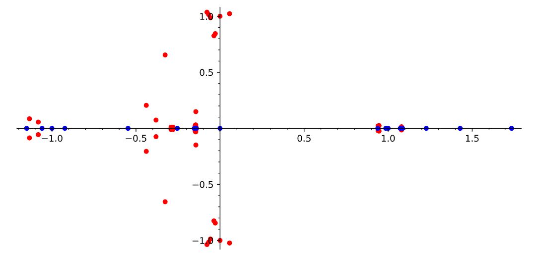
The singular solutions in this example, which can be accessed typing
singular(result),
all satisfy .
The numerical solution can be employed to obtain information on the geometric multiplicity of eigenvalues. The idea is the following: we generate new generic linear polynomials , append the polynomials to (10) and solve the system numerically. Observe that unlike , the polynomials are not affine linear, i.e., there is no degree .
Lemma 7.3.
Let be an affine linear polynomial, and for let be linear polynomials. If is a solution of the system
then is an eigenvalue with . If after adding a new generic linear polynomial to the system there is no solution with , then .
Therefore, we can continue adding generic linear polynomials until no solutions are found. All eigenvalues are found in this way, with the correct geometric multiplicity. We illustrate this fact in Example 7.4.
Example 7.4.
As we pointed out in Example 7.2, the unique eigenvalue obtained from a singular solution of (7.2) is . Therefore this is the only eigenvalue which might have geometric multiplicity higher than . To verify that this the case, we append to the system (7.2) a random linear polynomial and compute a solution numerically. We find solutions with , hence . Moreover, the system obtained adding another random linear polynomial does not admit any solution. We conclude that , and all the other eigenvalues have geometric multiplicity .
Funding
FG is supported by the National Science Center, Poland, project “Complex contact manifolds and geometry of secants”, 2017/26/E/ST1/00231, and acknowledges partial support by the fund FRA 2018 of University of Trieste – project DMG, funded by the MIUR Excellence Department Project awarded to the Department of Mathematics and Geosciences, University of Trieste. RM is supported by The Alan Turing Institute under the EPSRC grant EP/N510129/1. LV is funded by the Göran Gustafsson foundation.
Acknowledgments
We are grateful to the anonymous referee for the comments and suggestions that have greatly improved the first version of this paper. We thank Christian Kuehn (TUM) for the helpful comments and suggestions. We would like to thank Bernd Sturmfels (MPI MiS), who has always actively encouraged us to work together.
References
- [1] A. Banerjee and A. Char. On the spectrum of directed uniform and non-uniform hypergraphs. arXiv:1710.06367.
- [2] A. Banerjee, A. Char, and B. Mondal. Spectra of general hypergraphs. Linear Algebra and its Applications, 518:14–30, 2017.
- [3] A. Banerjee and S. Parui. On synchronization in coupled dynamical systems on hypergraphs. arXiv:2008.00469, 2020.
- [4] N. Bao, N. Cheng, S. Hernández-Cuenca, and V. P. Su. The quantum entropy cone of hypergraphs. SciPost Phys., 9(5):Paper No. 067, 39, 2020.
- [5] Á. Bodó, G.Y. Katona, and P.L. Simon. Sis epidemic propagation on hypergraphs. Bulletin of mathematical biology, 78(4):713–735, 2016.
- [6] P. Breiding and S. Timme. HomotopyContinuation.jl: A Package for Homotopy Continuation in Julia. In Mathematical Software – ICMS 2018, pages 458–465, Cham, 2018. Springer International Publishing.
- [7] A.E. Brouwer and W.H. Haemers. Spectra of graphs. Springer Science & Business Media, 2011.
- [8] F. Chung. Spectral graph theory. American Mathematical Soc., 1997.
- [9] C. Duan, L. Wang, and X. Li. Some Properties of the Signless Laplacian and Normalized Laplacian Tensors of General Hypergraphs. Taiwanese Journal of Mathematics, 24(2):265–281, 2020.
- [10] Y.-Z. Fan, T. Huang, Y.-H. Bao, C.-L. Zhuan-Sun, and Y.-P. Li. The spectral symmetry of weakly irreducible nonnegative tensors and connected hypergraphs. Transactions of the American Mathematical Society, 372(3):2213–2233, 2019.
- [11] C.J. Hillar and L.-H. Lim. Most Tensor Problems Are NP-Hard. J. ACM, 60(6), 2013.
- [12] S. Hu and Y. Ke. Multiplicities of tensor eigenvalues. Communications in Mathematical Sciences, 14:1049–1071, 2016.
- [13] J. Jost and R. Mulas. Hypergraph Laplace operators for chemical reaction networks. Advances in Mathematics, 351:870–896, 2019.
- [14] Jürgen Jost and Raffaella Mulas. Normalized Laplace operators for hypergraphs with real coefficients. J. Complex Netw., 9(1):Paper No. cnab009, 25, 2021.
- [15] M. Kivelä, A. Arenas, M. Barthelemy, J.P. Gleeson, Y. Moreno, and M.A. Porter. Multilayer networks. Journal of Complex Networks, 2(3):203–271, 07 2014.
- [16] S. Klamt, U.-U. Haus, and F. Theis. Hypergraphs and cellular networks. PLoS Comput Biol, 5(5):e1000385, 2009.
- [17] N. Lanchier and J. Neufer. Stochastic dynamics on hypergraphs and the spatial majority rule model. Journal of Statistical Physics, 151(1):21–45, 2013.
- [18] L. Lovász. Normal hypergraphs and the perfect graph conjecture. Discrete Mathematics, 2(3):253–267, 1972.
- [19] C. Ma, H. Liang, Q. Xie, and P. Wang. Some inequalities on the spectral radius of nonnegative tensors. Open Mathematics, 18(1):262–269, 2020.
- [20] B.D. MacArthur, R.J. Sánchez-García, and J.W. Anderson. Symmetry in complex networks. Discrete Applied Mathematics, 156(18):3525–3531, 2008.
- [21] C. Mariconda and A. Tonolo. Discrete Calculus: Methods for Counting. Springer, 2015.
- [22] R. Mulas, C. Kuehn, and J. Jost. Coupled dynamics on hypergraphs: Master stability of steady states and synchronization. Phys. Rev. E, 101:062313, 2020.
- [23] R. Mulas and D. Zhang. Spectral theory of Laplace operators on oriented hypergraphs. Discrete Mathematics, 344:112372, 2021.
- [24] X. Ouvrard, J.-M. Le Goff, and S. Marchand-Maillet. Adjacency and Tensor Representation in General Hypergraphs Part 1: e-adjacency Tensor Uniformisation Using Homogeneous Polynomials. arXiv:1712.08189.
- [25] X. Ouvrard, J.-M. Le Goff, and S. Marchand-Maillet. Adjacency and tensor representation in general hypergraphs. Part 2: Multisets, hb-graphs and related e-adjacency tensors. arXiv:1805.11952.
- [26] L. Qi. Eigenvalues of a real supersymmetric tensor. Journal of Symbolic Computation, 40(6):1302–1324, 2005.
- [27] L. Qi and Z. Luo. Tensor analysis. Society for Industrial and Applied Mathematics, Philadelphia, PA, 2017. Spectral theory and special tensors.
- [28] L. Qi and Y. Song. An even order symmetric B tensor is positive definite. Linear Algebra and its Applications, 457:303–312, 2014.
- [29] S. Ranshous, C.A. Joslyn, S. Kreyling, K. Nowak, N.F. Samatova, C.L. West, and S. Winters. Exchange pattern mining in the bitcoin transaction directed hypergraph. In International Conference on Financial Cryptography and Data Security, pages 248–263. Springer, 2017.
- [30] N. Reff. Spectral properties of oriented hypergraphs. Electron. J. Linear Algebra, 27, 2014.
- [31] N. Reff and L.J. Rusnak. An oriented hypergraphic approach to algebraic graph theory. Linear Algebra Appl., 437:2262–2270, 2012.
- [32] L.J. Rusnak. Oriented hypergraphs: Introduction and balance. The Electronic Journal of Combinatorics, 20, 2013.
- [33] J.-Y. Shao. A general product of tensors with applications. Linear Algebra and its applications, 439(8):2350–2366, 2013.
- [34] J.-Y. Shao, H.-Y. Shan, and B.-F. Wu. Some spectral properties and characterizations of connected odd-bipartite uniform hypergraphs. Linear and Multilinear Algebra, 63(12):2359–2372, 2015.
- [35] J.-Y. Shao, H.-Y. Shan, and L. Zhang. On some properties of the determinants of tensors. Linear Algebra and its Applications, 439(10):3057–3069, 2013.
- [36] Z.-K. Zhang and C. Liu. A hypergraph model of social tagging networks. Journal of Statistical Mechanics: Theory and Experiment, 2010(10):P10005, 2010.