Infrared Renormalons in Collider Processes
Abstract
Precise theoretical predictions are a key ingredient for an accurate determination of the structure of the Langrangian of particle physics, including its free parameters, which summarizes our understanding of the fundamental interactions among particles. Furthermore, due to the absence of clear new-physics signals, precise theoretical calculations are required in order to pin down possible subtle deviations from the Standard Model predictions. The error associated with such calculations must be scrutinized, as non-perturbative power corrections, dubbed infrared renormalons, can limit the ultimate precision of truncated perturbative expansions in quantum chromodynamics. In this review we focus on linear power corrections that can arise in certain kinematic distributions relevant for collider phenomenology where an operator product expansion is missing, e.g. those obtained from the top-quark decay products, shape observables and the transverse momentum of massive gauge bosons. Only the last one is found to be free from such corrections, while the mass of the system comprising the top decay products has a larger power correction if the perturbative expansion is expressed in terms of a short-distance mass instead of the pole mass. A proper modelization of non-perturbative corrections is crucial in the context of shape observables to obtain reliable strong coupling constant extractions.
1 Introduction
The Standard Model (SM) of particle physics encapsulates our understanding of the fundamental interactions among the elementary particles that constitute the building blocks of our universe. Particle colliders like the Large Electron-Proton collider (LEP) and the Large Hadron Collider (LHC) enable us to probe such fundamental laws at unprecedented precision, via comparison of accurate theoretical predictions and the experimental data. Hower the SM is known to be incomplete, as it does not include a description of gravity, it cannot explain the origin of its fundamental parameters, neutrino oscillations, matter–antimatter asymmetry, the nature of dark matter and dark energy… Many Beyond SM extensions have been proposed but no clear signal of new physics has been observed yet. In this scenario, we expect new physics to manifest only via subtle deviations from SM predictions. Thus, in order to pin down such deviations and improve the accuracy of the determinations on the parameters of the SM Lagrangian, the experimental data must be confronted with precise theoretical calculations.
Calculations for collider processes are performed as a perturbative expansion in the strong coupling , where the theoretical uncertainty mainly arises from the truncation of this series. However it is well-known that perturbative expansions in quantum field theory do not converge Dyson:1952tj, as a non-zero convergency radius will imply the validity of the theory also for negative values of the coupling constant, which instead prevents the existence of a stable vacuum. In particular, if we want to apply the method developed by Borel to resum factorially growing divergent series Borel to quantum chromodynamics (QCD), we are forced to introduce ambiguous terms that lead to power corrections of the order , with an hadronic scale, the hard-scattering scale and a positive integer. These power corrections are dubbed infrared renormalons as they are associated with the growth of the strong coupling constant at small scales11 1 Since the elecromagnetic coupling constant increases at large energies, quantum electrodynamics is instead affected by ultraviolet renormalons.. The existence of an Operator Product Expansion (OPE) provides a safe guideline for the classification of such power corrections, due to the correspondance between power-suppressed terms caused by the bad large-order behaviour of QCD and those associated from higher twists operators. Thus, we can see that power corrections arise because perturbation theory is not complete and we need to include non-perturbative contributions to recover the full result Mueller:1993pa.
Unfortunately, there is no OPE for the majority of the kinematic distributions measured at colliders, so we need to compute the perturbative coefficients at all orders to assess for example the presence of linear power corrections (), which can lead to an ambiguity at the percent level for hard scales of the order of the mass, possibly significantly limiting the ultimate uncertainty of theoretical predictions. This can be done in the limit of an infinite and negative number of quark flavours , where at the end one performs the replacement , where is the first coefficient of the QCD beta function
| (1) |
with being the real number of light flavours of the theory Beneke:1994qe. This procedure encapsulates an explicit dependence on the running of the strong coupling, which is the responsible of the factorial growth of the perturbative expansion, and for this reason it has been successfully employed in several contests, like the pole mass ambiguity Ball:1995ni, event shapes Nason:1995np, Drell-Yan (DY) production Beneke:1995pq, fragmentation functions in annihilation Dasgupta:1996ki. An exhaustive description of the phenomenological applications is discussed in Sec. 5 of Ref. Beneke:1998ui, which constitutes a comprehensive and detailed review on the topic of renormalons. In this contribution we instead only focus on most recent phenomenological applications.
In Sec. 2 we briefly summarize the Borel summation technique, emphasizing the residual ambiguity related to perturbative series in QCD. In Sec. 3 we introduce the large- limit to assess the presence of power corrections, and we discuss the application to the pole mass (Sec. 3.1). In Sec. 3.2 we illustrate how this method can be applied numerically for evaluating any arbitrary infrared-safe observable, following the proposal of Refs. FerrarioRavasio:2018ubr; FerrarioRavasio:2020guj. The application to the case of top-quark production and decay is summarized in Sec. 4. In Sec. 5 this method is employed to investigate the presence of linear renormalons in the transverse-momentum distribution of a gauge boson recoiling against a hard jet. In Sec. 6 we discuss the evaluation of non-perturbative corrections for shape observables in collisions. Conclusions and outlooks are summarized in Sec. 7.
2 Factorially divergent series
Let us consider a factorially-divergent series
| (2) |
where is the small (and positive) expansion parameter and is a real number. The smallest term of the series is reached for , i.e. for and, if , has size
| (3) |
Borel devised a summation method for alternating factorially-divergent series Borel, which allows us to rewrite eq. (2) for as
| (4) |
which is well defined as there are no poles on the integration range. We immediately realise that if we want to use the Borel summation also when is negative, i.e. if and the coefficients in eq. (2) have all the same sign, there is a pole on the integration path: to interpret eq. (5) as estimate of the resummed expression we thus need to add a small imaginary part to the denominator of the integrand. The sign of this imaginary part is arbitrary, indeed we can define
| (5) |
An estimate of the ambiguity of the resummed series is thus given by
| (6) |
We see that this ambiguity is identical to the minimum term of the perturbative series given in eq. 3, modulo a normalization factor .
Let us now focus to QCD, where the expansion paramer is now the strong coupling evaluated at a hard scale
| (7) |
where is given by eq. (1) and is the energy scale at which becomes infinity. The value of the strong coupling at another scale can be expressed as a function of :
| (8) |
When performing all-orders calculations, a large number of contributions can be resummed by evaluating the next-to-leading-order (NLO) term at a running scale. This means that the contribution to an infrared-safe observable is approximatively given by
| (9) |
where is a positive integer as required from the infrared-safety property of the observable. Thus, since the first coefficient of the QCD -function is positive, resumming soft emissions at all orders leads to same-sign factorially divergent series, with minimum term located at . The smallest term of the series and the ambiguity on the Borel-resummed result are proportional to
| (10) |
Thus we see that the nature of the power corrections induced by the bad large-order behaviour of QCD is encoded in the value of the parameter appearing in eq. (9). The largest and most worrisome corrections arise for and are dubbed linear infrared renormalons.
3 The large-number-of-flavour approximation
In absence of an OPE, we need to perform an all-order calculation to infer the value of which appears in eq. (9). Higher-order corrections are accessible up to all orders in the coupling when considering the limit of a large number of flavours , where the only contributions to be considered arise from the insertion of fermion loops in the gauge-field propagator, since they involve powers of . This implies that free gluon propagator must be replaced with the dressed one:
| (11) |
The self-energy correction is ultraviolet divergent, but usually no additional subtractions beyond those contained in the renormalized QCD Lagrangian are required, so we can evaluate using the renormalized fermion-loop expression22 2 When evaluating quantities which explicitly involve ultraviolet divergences, like the difference between the pole and the mass, we need to compute in dimensions (or using another regularization procedure) and extract the finite part of the result only after having carried out all the other integrations.
| (12) |
where is a renormalization-scheme dependent constant, equal to in the scheme. This procedure was originally proposed for quantum electrodynamics (QED) Lautrup:1977hs, but since the pre-factor of eq. (12) coincides with the fermionic contribution of the full QCD -function (1), we can adopt this method also for QCD if at the end perform the replacement
| (13) |
to recover the non-abelian property of the theory Beneke:1994qe. This naive non-abelianization is often referred as the large- approximation.
3.1 Application: top-quark pole mass
To gauge the validity of this method with a concrete example, we consider the relation between the () and the pole mass () for the top quark. This relation is known up to order Marquard:2015qpa
| (14) |
From eq. (14) it is already evident that the coefficients are affected by a factorial growth. This series can be computed at all-orders in the large- approximation, yielding Ball:1995ni
| (15) |
Comparing eqs. (14) and (15), we can immediately notice that the coefficient computed in this approximation is only 20% larger then the exact one, as expected from the observation that the factorial growth is already visible from eq. (14).
The asymptotic behaviour of the coefficients can also be inferred assuming the resummed series is renormalization-scale independent Beneke:1994rs
| (16) |
where and can be expressed in terms of the full QCD -function coefficients. Since , we immediately notice a similarity with eq. 9 with , thus the pole-mass definition is affected by a linear renormalon. The only unknown ingredient in eq. (16) is the overall normalization . The authors of Ref. Beneke:2016cbu fitted the value of from the already-known perturbative coefficients and used the asymptotic formula in eq. (16) to estimated the missing higher-order contributions, finding
| (17) |
We can notice a remarkable agreement between the large-order terms computed in eq. (17) and those obtained applying the large- approximation. Thus this confirm that resumming all-order corrections in provides us a simple but yet valid approximation to infer the main properties of the large-order behaviour of QCD.
We can use the smallest term of the series in eq. (17) to gauge the ambiguity of the Borel-resummed series
| (18) |
however this number is obtained neglecting charm- and bottom-quark mass effects. By including them, the estimated ambiguity becomes 110 MeV Beneke:2016cbu, while the approach adopted by the authors of Ref. Hoang:2017btd leads to 250 MeV. If the top pole-mass ambiguity is of the order of 100 or 200 MeV is not crucial yet, given that the most accurate LHC measurements reach 500 MeV error Khachatryan:2015hba; Aaboud:2018zbu. However, having a method that allows us to determine the nature of the non-perturbative correction for a generic infrared-safe observable can help us assessing how the pole-mass ambiguity propagates to top-dependent observables. We can also apply this method in the context of shape observables, where non-perturbative effects are large and need a proper modelization, or to kinematic distributions like the transverse momentum of gauge bosons, to determine the presence or the absence of linear terms.
3.2 Practical implementation
(b) (v) () ()
In this section we describe how to compute all-orders corrections in the large- limit for a generic process which does not contain any gluon at the lowest perturbative order, following the recipe introduced in Ref. FerrarioRavasio:2018ubr. The expression for a generic observable function of the final-state kinematics for is given by
| (19) |
where corresponds to the Born cross section, corresponds to the virtual cross section, comes from the emission of an onshell gluon and is obtained from the emission of an offshell gluon which splits into a pair. Examples of the Feynman diagrams contributing to , , and are given in Fig. 1, where the solid red blob represents the insertion of the fermionic loops in all possible ways, and can be defined with this recursive relation
| (20) |
We stress that in the contribution of Fig. 1 we can always assume that the pair arising from the gluon splitting has a different flavour from other quarks already present in the LO (b) diagram, as interference effects would be suppressed by one inverse power of . We label with and the phase space for the Born configuration and for the process containing an additional gluon , while is the phase space for the contribution with an additional pair, which can be conveniently rewritten as
| (21) |
where denotes an offshell gluon with mass and is the phase space for the decay.
Manipulating eq. (19) and performing the replacement in eq. (13) we get FerrarioRavasio:2018ubr
| (22) |
where is the LO prediction,
| (23) |
with a renormalization-scheme dependent constant that we choose to be equal to
| (24) |
so that corresponds to in the Catani-Marchesini-Webber (CMW) scheme Catani:1990rr, and
| (25) |
where and are the corrections to the LO cross section, computed with a gluon of mass , while corresponds to the () contribution of Fig. 1 without any blob insertion in the offshell gluon propagator. The dependence cancels in the ratio , so that is effectively independent. For large , so the integral in eq. (22) is UV convergent. For vanishing
| (26) |
which corresponds to the usual NLO corrections computed using a mass regularization for processes which do not contain incoming partons. If we consider a process with an incoming quark leg, eq. (26) contains divergent terms due to the mis-cancellation of initial-state collinear singularities. We thus need to include to the term FerrarioRavasio:2020guj
| (27) |
where is the momentum of the incoming proton, while is the energy fraction of the quark which enters the LO hard scattering process, is the factorization scale33 3 The dependence cancels in the integral if the PDF evolution is also computed in the large- approximation., is the parton distribution function (PDF) for the incoming quark and corresponds to the correction to the Deep Inelastic Scattering (DIS) cross section, computed with a massive gluon, normalised to the LO prediction, stripping all the PDF factors Beneke:1995pq. In this way smoothly approaches the conventional NLO result where the PDF has been renormalized in the DIS scheme.
We notice that if
| (28) |
the small- contribution to (22) gives rise to the following perturbative series
| (29) |
which has minimum equal to , or equivalently leads to a Borel-resummed result with ambiguity . Thus, a linear- in leads to linear renormalons, while if the derivative in (28) is zero, only higher power corrections will appear. The term included in eq. 27 does not include any linear -dependence, as the form factor which gives the DIS cross section obeys an OPE where power corrections are controlled by higher twist operators, and the dominant power corrections, corresponding to twist 4, are quadratic.
The ingredients appearing in eq. (22) are not new, indeed an effective coupling similar to the one in eq. (23) naturally arises when applying dispersion relations to bubble diagrams appearing in the virtual diagrams (see Ref. Beneke:1998ui and references therein). Furthermore infrared renormalons in shape observables were typically inferred convoluting radiative corrections due to soft emissions with an effective coupling Dokshitzer:1995zt. The first line of eq. (25) corresponds to the NLO calculation performed using a gluon of mass , as a matter of fact linear power corrections were originally inferred using the “massive gluon method”, which was used for example by the authors of Ref. Beneke:1995pq to show that the DY cross section is not affected by linear renormalons. The second line of eq. (25) is identical to zero for inclusive observables insensitive to the gluon splitting appearing in the contribution of Fig. 1, but it must be included for observables sensitive to the kinematics of the whole final state, as already shown in Ref. Nason:1995np. Eq. (22) brings all these ingredients together and allows us to compute results in the large- approximation exactly, using a combination of analytic and numerical methods, in such a way that any arbitrary process, which does not contain gluons at LO, can be computed.
4 All-order corrections for top-mass determinations
The mass of the top quark is one key parameters of the standard model, as it is important non only for the top phenomenology, but also because it largely affects many other parameters (e.g. gauge boson masses, Higgs trilinear coupling). As already discussed in Sec. 3.1, the pole mass definition is affected by a linear renormalon and hence has an ambiguity of roughly 100–200 MeV Beneke:2016cbu; Hoang:2017btd. In Ref. FerrarioRavasio:2018ubr we investigated the asymptotic behaviour of kinematic distributions of the top decay-products computed in terms of the pole mass and of the mass (that we can consider as a proxy of all the short-distance mass schemes) in a simplified theoretical framework where we understand some aspects concerning the non-perturbative corrections to the pole mass. To achieve this task, formula (22) was applied to the process of single-top production and decay, i.e. . The calculation of was performed in the complex pole scheme, with , in order to include finite top-width () effects and interferences between radiative corrections in the production process , and in the top decay . We stress that eq. (22) cannot be evaluated directly in four dimensions if the top mass is renormalized in the scheme, as would still contain ultraviolet divergencies. Details on the computation of in the scheme can be found in Sec. 3.3 of Ref. FerrarioRavasio:2018ubr, however if we are only interested in the small- behaviour we can write
| (30) |
where the coefficient arises from the computation of the one-loop top self-energy correction with a massive gluon.
When computing the total cross section, the linear- sensitivity is given only by the insertion of the pole-mass conterterm, which cancels exactly with the extra term in eq. (30) when using the scheme. This cancellation takes place irrespectively of the value of , and hence we can affirm that the total cross section in the scheme is always free from linear renormalons, even if the calculation is performed in the narrow-width approximation (NWA). The smallest term of the series in the pole scheme is reached for .
If we want to define a fiducial cross section, requiring for example the presence of two different and jets, we introduce a linear- slope which diverges as , where is the jet radius, irrespectively of the jet algorithm and of the mass scheme used, as we become sensitive to jet-related renormalons Dasgupta:2007wa. This is illustrated in Fig. 2, where we show the function computed for different values of the jet radius in the pole scheme (left panel) and its derivative for , both in the pole and in the scheme. If we choose , the slope in the scheme is much smaller than in the pole scheme, thus yielding an improved perturbative convergence.
Interestingly, leptonic observables (in the collision frame) expressed in terms of the mass are linear-renormalon free only if a non-zero value is adopted44 4 Leptonic observables computed in the top frame are free from linear renormalons once the mass is used because an OPE forbids such power corrections.. Indeed the presence of a finite GeV modifies the behaviour of the integral in eq. 22 for scales smaller than , preventing the top from being onshell. If we expand the effective coupling (23) in series of , with GeV, we realise that values larger than give the dominant corrections till order , so we need to compute many perturbative orders before realizing the improved perturbative convergence of the with respect to the pole scheme. This is illustrated also in Tab. 1, where the coefficients of the perturbative expansion
| (31) |
are shown.
| [GeV] | ||||
|---|---|---|---|---|
| pole scheme | scheme | |||
| 0 | ||||
| 1 | ||||
| 2 | ||||
| 3 | ||||
| 4 | ||||
| 5 | ||||
| 6 | ||||
| 7 | ||||
| 8 | ||||
| 9 | ||||
| 10 | ||||
| 11 | ||||
| 12 | ||||
Furthermore leptonic observables have a reduced top-mass sensitivity compared to other observables traditionally used to infer like, for example, the mass of the system comprising the top decay products . For example, for GeV, GeV and GeV we have that at LO
| (32) |
This means that an uncertainty on the energy of the boson will lead to an uncertainty of on the value of the top mass .
For this reason, we investigate the linear- sensitivity of the function associated with the average value of the mass of the -boson and -jet system . If we choose and we perform the calculation in NWA, we notice that , so there are no linear power-corrections. This is due to the fact that if and we are inclusive enough in the definition of the jet, the mass of the system comprising the top decay products is identical to the top pole-mass, which is not displaced by any radiative corrections by definition. This means , which implies that the perturbative series in the pole scheme is well defined and all the corrections are 0 for any . If instead we use the scheme, we find the same factorially-divergent series that relates the pole and the mass. This means that the observable contains an intrinsic physical renormalon which cancels with the pole-mass one. As already discussed for the case of leptonic observables, the presence of a finite top-width modifies the large-order behaviour of the series, as the interference between the radiation in the production process and the top decay spoils this cancellation. This is shown in the left panel of Fig. 3. However, we still find that for using the pole scheme yields a smaller ambiguity as the power correction in the scheme is roughly three times larger, as illustrated in the right panel of Fig. 3.
5 Transverse momentum of massive gauge bosons
The transverse momentum of the -boson is one of the most precise observables measured at the LHC, due to its large yield and its clear leptonic signature, and the experimental error associated with the normalised distribution is at sub-percent level in the low-intermediate values of the transverse momentum Sirunyan:2019bzr; Aad:2019wmn. The current state of the art for the theoretical prediction is given by NNLO+N3LL′ Re:2021con, where the error is instead at the percent level. Resummation effects have been proven to have a large effect in the region where the boson transverse momentum is small. Non-perturbative corrections associated with the low- region have been extensively studied Dokshitzer:1978yd; Parisi:1979se; Collins:1984kg; Scimemi:2016ffw, and no linear power-correction was found. This has a rather intuitive explanation since in this context they can be modelled as a gaussian transverse momentum smearing. Since this smearing is azimuthally symmetric, its first-order effects cancel out, leaving only quadratic corrections.
For moderate values of , the boson recoils against a coloured final-state particle, and reliable theoretical predictions can be obtained from the calculation of +jet production at NNLO Boughezal:2015ded; Ridder:2015dxa. The presence of a linear correction of the order is particularly worrisome as it can lead to a non-perturbative correction comparable to the current theoretical uncertainty and pose a serious limit on the ultimate uncertainty one can aim at with a pure perturbative calculation. Conversely to the inclusive DY case, when the boson is produced in association with a hard jet, the soft-radiation pattern is not symmetric and this azimuthally asymmetry can in principle prevent the cancellation of linear power-corrections. This is illustrated in the left panel of Fig. 4, which portrays the process , where additional soft gluons can only be emitted from two initial-final dipoles.
(a) (b)
Unfortunately, due to the presence of a gluon at the lowest perturbative order, such process cannot be computed using eq. (22). For this reason in Ref. FerrarioRavasio:2020guj we considered instead (right panel of Fig. 4), which still features the presence of an initial-final dipole and thus an azimuthally-asymmetric radiation pattern. QED divergences are removed using the FKS subtraction implemented in POWHEG BOX framework Frixione:2007vw; Alioli:2010xd; Jezo:2015aia that we use for the numerical evaluation of . We compute the total cross section imposing a minimum cut and we do not find any numerical evidence of linear- terms. We do not find linear renormalons also for the -rapidity distribution computed with such cut, as already found for the more inclusive DY production Dasgupta:1999zm. This is illustrated in Fig. 4, where we show the value of associated with the fiducial cross section obtained imposing and an asymmetric cut on for several values of the gluon mass . To obtain the functional form of , and hence the slope for , we use the following interpolating function
The fitted coefficient for all the cuts we have considered is always compatible with zero.
We can thus conjecture that linear power corrections only arise from soft radiation that, at least in the leading colour approximation, can be emitted only from dipoles. If we integrate over the whole phase space of the emitting dipole, such linear terms cancel. Further analytical work is needed in order to put these conjectures on more solid ground Caola.
6 Shape observables
The simplest observables measured at lepton colliders are event shape observables like the thrust
| (33) |
and the -parameter
| (34) |
with the four-momenta of all the final-state particles and , as they provide us a continuous measure of deviation from lowest-order process and can serve as a QCD “laboratory” to perform, for example, strong coupling-constant fits.
Non-perturbative corrections are crucial to perform extractions and they can be inferred using a renormalon-inspired dispersive approach. Such corrections are modelled as a negative shift in the perturbative distribution Dokshitzer:1997ew, and they are computed considering the change in the shape obserable induced by a soft emission starting from the two-jet configuration Dokshitzer:1995zt, where the strong coupling is replaced with an infrared-regular effective strong coupling similar to the one in eq. (23). The authors of Ref. Nason:1995np investigated the effect of infrared renormalons upon the thrust using the large- limit, showing the additional branching of a soft gluon (namely the second line of eq. (25)) leads to a larger shift than the naive estimate one would obtain simply considering the effect of a soft emission. One can however recover the complete result predicted by the large- method by applying a corrective factor, usually dubbed as Milan factor Dokshitzer:1997iz; Dokshitzer:1998pt; Dasgupta:1999mb, which is the same for the same class of observables and in particular is identical for the thrust and the -parameter. In addition to the final splitting considered by the large- approximation, the inclusion of the Milan factor also accounts explicitly for the final state with two soft gluons, which gives a sizeable contribution that cannot be captured by the naive non-abelianization procedure , as the two branchings lead to different kinematics. Alternatively, one could use Monte Carlo (MC) event generators to estimate such non-perturbative corrections Bethke:2008hf; Dissertori:2009ik; OPAL:2011aa; Kardos:2018kqj. This approach has however been criticised since the separation between perturbative and non-perturbative components in a MC is rather arbitrary. Furthermore, the hadronization model is tuned on parton showers which provide a less accurate description of the perturbative component.
Current extractions from shape observables, where hadronization corrections are extracted from a renormalon-inspired analytic model, are roughly three standard deviations smaller the world average pdg, for example
- •
from the thrust distribution Abbate:2010xh;
- •
from the -parameter distribution Hoang:2015hka.
The authors of Ref. Luisoni:2020efy have suggested that this could be due to the fact that measurements are usually performed away from the two-jet limit, where the non-perturbative shifts and are estimated. Indeed the shift in the cumulant from the -parameter distribution
| (35) |
computed for , which corresponds to the three-jet symmetric point, is roughly half of the value for
| (36) |
This number is obtained by noticing that there is a Sudakov shoulder at , so one could estimate non perturbative corrections in the same fashion as done for the singular point. As noted by the authors of Ref. Luisoni:2020efy, that procedure is able to give a rigorous prediction only at the singular configurations, , not at other points of the spectrum, because different recoil prescriptions employed to model the kinematic of soft emissions can lead to different linear terms.
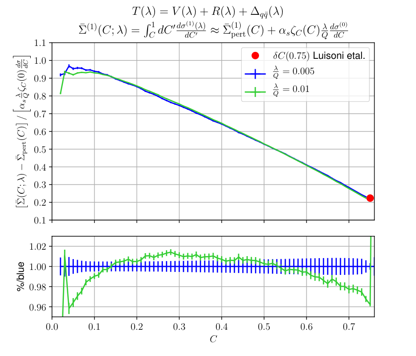
We can however extract the dependence of the shift on the geometry of the event in the large- limit, allowing us to investigate also configurations and shape observables which do not feature additional Sudakov shoulders. Since this abelian method works only if there are no gluons at the lowest perturbative order, to move away from the two-jet limit we can consider the configuration as LO process Caola. QED divergencies are subtracted using the same procedure employed in Ref. FerrarioRavasio:2020guj. We thus compute the function for the integrated cross section with a lower cut on or for a small value of , and then subtract , which corresponds to the standard correction to the LO prediction. Form eq. (35) we see that to extract the non-perturbative shift we can just divide the difference by the LO differential distribution computed for the 3-jet configuration . The result, normalized by the value of and by the non-perturbative shift computed in the two-jet limit55 5 This is the shift in the function, that needs to be convoluted with an effective coupling to get the full result, and thus is different from the shifts in eq. (36). However this is not necessary if we are just interested in assessing the dependence on the geometry of the event, i.e. for .
| (37) |
is shown in the upper panels of Fig. 6 for the -parameter (left) and the thrust (right). From the bottom panels we see that the curves computed with different small values of agree very well between each other, and the differences are compatible with additional suppressed quadratic power corrections. We also observe that, by reducing the value of , the shift computed for a low cut on or converges to the values in eq. (37). From the left panel of Fig. 6 we notice that the shift in is consistent with , which corresponds to the value found in Ref. Luisoni:2020efy for . We stress that we do not need a Sudakov shoulder to predict the linear- sensitivity, so we are also able to compute for any values of . These findings support the issue raised in Ref. Luisoni:2020efy that non-perturbative corrections in shape observables depend on the geometry of the event.

7 Conclusion and Outlooks
In the present contribution we reviewed the basic properties of linear power-corrections affecting kinematic distributions at colliders. Power corrections originate from the bad large-order behaviour of QCD, and signal the incompleteness of perturbative expansions and the need for the inclusion of non-perturbative corrections to recover the full result. For the majority of the kinematic distributions measured at LEP and at the LHC there is no OPE, so one needs to use approximations to perform all-orders calculations in QCD to infer the large-order behaviour and hence the non-perurbative corrections. All-order corrections become accessible in the large- limit, with being a fictitious number of light flavours. To recover the non-abelian property of QCD, at the end of the calculation one performs the replacement. Since infared renormalons are mainly caused by the divergence of the strong coupling at small scales, this procedure, which encapsulates an explicit dependence of the running of the strong coupling via the coefficient, provides us a simple but yet powerful way to assess the presence of linear corrections. In particular in this contribution we focused on some recent phenomenological applications of this method.
- •
Single-top production and decay FerrarioRavasio:2018ubr. Inclusive observables that do not depend upon the kinematics of the coloured final states, like the total cross section or leptonic observables, should be computed in the scheme (or in any other short distance mass scheme). However, if one employs the NWA, leptonic observables will still be affected by linear renormalons. If we instead want to calculate the mass of the top decay products, the pole mass yields a better perturbative convergence as it allows for a partial cancellation between the pole-mass renormalon and the physical one present in the intrinsic definition of the observable. This cancellation is exact in the limit of a vanishing top-width and if we are inclusive enough in the definition of the -jet arising from the top decay. Indeed, if we define the -jet using a small jet radius , we are strongly affected by jet-related linear corrections, which inversely proportional to , irrespectively of the mass prescription adopted.
- •
The transverse momentum of the -boson produced in association with a hard jet in hadronic collisions FerrarioRavasio:2020guj. For this observable we do not find any numerical evidence of a linear sensitivity despite the absence of an azimuthally-symmetric radiation pattern. This finding is not altered by the imposition of additional asymmetric rapidity cuts.
- •
Shape observables, where the estimate of hadronization effects is important to perform reliable extractions of the strong coupling. The authors of Ref. Luisoni:2020efy have raised the issues that measurements are performed away from the two-jet limit, where non-perturbative corrections are inferred, considering explicitly the case of . By studying the process , we are able to confirm their finding and make predictions for any shape-observable, however without the inclusion of non-perturbative corrections proportional to Caola.
Further analytical work is needed in order to formulate an analytic argument to explain the cancellation of linear power-corrections for processes where the soft-radiation pattern is not symmetric. This would also allow a major understanding of the underlying mechanisms that lead to the presence or absence of renormalon effects in collider physics. Sec. 6 contains preliminary results that will be published in Ref. Caola.
Acknowledgements
I want to thank Irinel Caprini and Diogo Rodrigues Boito for the invitation to contribute to the special issue “Renormalons and Hyperasymptotics in QCD”. The majority of the material presented in this contribution is obtained in collaboration with Fabrizio Caola, Giovanni Limatola, Kirill Melnikov, Paolo Nason and Carlo Oleari, to whom I am very grateful. I also want to acknowledge Pier F. Monni and Gavin P. Salam for useful discussions and comments on the manuscript. This work is supported by the European Research Council (ERC) under the European Union’s Horizon 2020 research and innovation program (grant agreement No. 788223, PanScales).
References
- (1) F. J. Dyson, Phys. Rev. 85 (1952), 631-632
- (2) E. Borel, (1899), Ann. Sci. Éc. Norm. Supér., Series 3, 16: 9–131
- (3) A. H. Mueller, Phys. Lett. B 308 (1993), 355-359
- (4) M. Beneke and V. M. Braun, Phys. Lett. B 348 (1995), 513-520
- (5) P. Ball, M. Beneke and V. M. Braun, Nucl. Phys. B 452 (1995), 563-625
- (6) P. Nason and M. H. Seymour, Nucl. Phys. B 454 (1995), 291-312
- (7) M. Beneke and V. M. Braun, Nucl. Phys. B 454 (1995), 253-290
- (8) M. Dasgupta and B. R. Webber, Nucl. Phys. B 484 (1997), 247-264
- (9) M. Beneke, Phys. Rept. 317 (1999), 1-142
- (10) S. Ferrario Ravasio, P. Nason and C. Oleari, JHEP 01 (2019), 203
- (11) S. Ferrario Ravasio, G. Limatola and P. Nason, (2020), arXiv:2011.14114
- (12) B. E. Lautrup, Phys. Lett. B 69 (1977), 109-111
- (13) P. Marquard, A. V. Smirnov, V. A. Smirnov and M. Steinhauser, Phys. Rev. Lett. 114 (2015) no.14, 142002
- (14) M. Beneke, Phys. Lett. B 344 (1995), 341-347
- (15) M. Beneke, P. Marquard, P. Nason and M. Steinhauser, Phys. Lett. B 775 (2017), 63-70
- (16) A. H. Hoang, C. Lepenik and M. Preisser, JHEP 09 (2017), 099
- (17) V. Khachatryan et al. [CMS], Phys. Rev. D 93 (2016) no.7, 072004
- (18) M. Aaboud et al. [ATLAS], Eur. Phys. J. C 79 (2019) no.4, 290
- (19) S. Catani, B. R. Webber and G. Marchesini, Nucl. Phys. B 349 (1991), 635-654
- (20) Y. L. Dokshitzer and B. R. Webber, Phys. Lett. B 352 (1995), 451-455
- (21) M. Dasgupta, L. Magnea and G. P. Salam, JHEP 02 (2008), 055
- (22) A. M. Sirunyan et al. [CMS], JHEP 12 (2019), 061
- (23) G. Aad et al. [ATLAS], Eur. Phys. J. C 80 (2020) no.7, 616
- (24) E. Re, L. Rottoli and P. Torrielli,
- (25) Y. L. Dokshitzer, D. Diakonov and S. I. Troian, Phys. Lett. B 79 (1978), 269-272
- (26) G. Parisi and R. Petronzio, Nucl. Phys. B 154 (1979), 427-440
- (27) J. C. Collins, D. E. Soper and G. F. Sterman, Nucl. Phys. B 250 (1985), 199-224
- (28) I. Scimemi and A. Vladimirov, JHEP 03 (2017), 002
- (29) R. Boughezal, J. M. Campbell, R. K. Ellis, C. Focke, W. T. Giele, X. Liu and F. Petriello, Phys. Rev. Lett. 116 (2016) no.15, 152001
- (30) A. Gehrmann-De Ridder, T. Gehrmann, E. W. N. Glover, A. Huss and T. A. Morgan, Phys. Rev. Lett. 117 (2016) no.2, 022001
- (31) S. Frixione, P. Nason and C. Oleari, JHEP 11 (2007), 070
- (32) S. Alioli, P. Nason, C. Oleari and E. Re, JHEP 06 (2010), 043
- (33) T. Ježo and P. Nason, JHEP 12 (2015), 065
- (34) M. Dasgupta, JHEP 12 (1999), 008
- (35) F. Caola, S. Ferrario Ravasio, G. Limatola, K. Melnikov, P. Nason, in preparation.
- (36) Y. L. Dokshitzer and B. R. Webber, Phys. Lett. B 404 (1997), 321-327
- (37) Y. L. Dokshitzer, A. Lucenti, G. Marchesini and G. P. Salam, Nucl. Phys. B 511 (1998), 396-418 [erratum: Nucl. Phys. B 593 (2001), 729-730]
- (38) M. Dasgupta, L. Magnea and G. Smye, JHEP 11 (1999), 025
- (39) Y. L. Dokshitzer, A. Lucenti, G. Marchesini and G. P. Salam, JHEP 05 (1998), 003
- (40) S. Bethke et al. [JADE], Eur. Phys. J. C 64 (2009), 351-360
- (41) G. Dissertori, A. Gehrmann-De Ridder, T. Gehrmann, E. W. N. Glover, G. Heinrich, G. Luisoni and H. Stenzel, JHEP 08 (2009), 036
- (42) G. Abbiendi et al. [OPAL], Eur. Phys. J. C 71 (2011), 1733
- (43) A. Kardos, S. Kluth, G. Somogyi, Z. Tulipánt and A. Verbytskyi, Eur. Phys. J. C 78 (2018) no.6, 498
- (44) J. Huston, K. Rabbertz, G. Zanderighi. 2019 update to the quantum Chromodynamics review (2019). URL http: //pdg.lbl.gov/2019/reviews/rpp2019-rev-qcd.pdf
- (45) R. Abbate, M. Fickinger, A. H. Hoang, V. Mateu and I. W. Stewart, Phys. Rev. D 83 (2011), 074021
- (46) A. H. Hoang, D. W. Kolodrubetz, V. Mateu and I. W. Stewart, Phys. Rev. D 91 (2015) no.9, 094018
- (47) G. Luisoni, P. F. Monni and G. P. Salam, Eur. Phys. J. C 81 (2021) no.2, 158