H-FL: A Hierarchical Communication-Efficient and Privacy-Protected Architecture for Federated Learning
Abstract
The longstanding goals of federated learning (FL) require rigorous privacy guarantees and low communication overhead while holding a relatively high model accuracy. However, simultaneously achieving all the goals is extremely challenging. In this paper, we propose a novel framework called hierarchical federated learning (H-FL) to tackle this challenge. Considering the degradation of the model performance due to the statistic heterogeneity of the training data, we devise a runtime distribution reconstruction strategy, which reallocates the clients appropriately and utilizes mediators to rearrange the local training of the clients. In addition, we design a compression-correction mechanism incorporated into H-FL to reduce the communication overhead while not sacrificing the model performance. To further provide privacy guarantees, we introduce differential privacy while performing local training, which injects moderate amount of noise into only part of the complete model. Experimental results show that our H-FL framework achieves the state-of-art performance on different datasets for the real-world image recognition tasks.
1 Introduction
Federated learning (FL) is a promising distributed paradigm for training a shared model while keeping all the training data localized [\citeauthoryearYang et al.2019, \citeauthoryearKairouz et al.2019, \citeauthoryearKonečnỳ et al.2016]. However, FL always involves expensive communication and privacy concerns in order to maintain a great model performance [\citeauthoryearLi et al.2020, \citeauthoryearZhang et al.2021]. Therefore, how to find a great balance among model performance, communication overhead and privacy requirements is a long-term, challenging goal.
From a methodological standpoint, DGC [\citeauthoryearLin et al.2017] and FetchSGD [\citeauthoryearRothchild et al.2020] have given a good trade-off between communication overhead and model performance by compressing the gradients and giving some corrections. NbAFL [\citeauthoryearWei et al.2020] and DP-FedAVG [\citeauthoryearMcMahan et al.2017b] provide strong privacy guarantees via differential privacy without undue sacrifice on model performance. SplitNN [\citeauthoryearVepakomma et al.2018] can achieve higher model performance in contrast to the aforementioned methods while protecting sensitive raw data. All these works try to make some trade-offs from different perspectives. However, when treating model performance, communication overhead and privacy requirements as a whole perspective, it will introduce a completely new contradiction: the contradiction between communication overhead and privacy requirements while maintaining model performance in a certain level. Since when utilizing some privacy protection methods such as differential privacy and secure multiparty computing to provide privacy guarantees, it will inevitably introduce additional communication overhead directly or slow down the convergence rate, leading to requiring extra communication rounds for FL algorithms to converge. Therefore, we cannot just do simple combinations from different perspectives.
In this paper, we develop a hierarchical federated learning architecture (H-FL) as shown in Figure 1. To counter-weigh the degradation of model performance due to statistic heterogeneity of the training data, H-FL introduces mediators to reconstruct the local distributions. We cluster the clients according to the KL divergence between local distributions of each client and a uniform distribution, as well as the information entropy of the local distributions, and then reallocate them to different mediators. When participating in federated tasks, H-FL selects mediators rather than clients and each mediator rearranges its clients to perform the training tasks in order to alleviate the statistic heterogeneity. In addition, we design a compression-correction mechanism to reduce the communication overhead without sacrificing the model performance, which significantly compresses the extracted features of the clients uploaded to mediators and corrects the corresponding gradients download from the mediators. To further provide privacy guarantees for clients, we introduce differential privacy when each client conducts its local training.

Our contributions can be summarized as following:
- •
To the best of our knowledge, H-FL is the first attempt to treat model performance, communication overhead and privacy requirements as a whole perspective to find a great balance among them.
- •
We devise a runtime distribution reconstruction strategy to alleviate the statistic heterogeneity of the training data while not compromising user privacy. Moreover, we design a compression-correction mechanism to reduce the communication overhead without sacrificing the model performance.
- •
Extensive experiments on different datasets show that our H-FL architecture achieves state-of-the-art performance on federated image recognition tasks.
2 Related Research
Federated learning is a collaborative distributed learning paradigm which removes the necessity to pool the raw data out from local clients. Specifically, FedAVG algorithm proposed in [\citeauthoryearMcMahan et al.2017a] aims to reduce the communication overhead while maintaining a good performance of the model on non-IID (Independent and identically distributed) training data, which is used as our baseline in Section 4. Furthermore, concurrent works such as [\citeauthoryearLin et al.2018, \citeauthoryearSattler et al.2019] have focused on further reducing communication overhead in FL via gradient sparsification, and propose solutions to counter-weigh the reduction in accuracy due to the statistic heterogeneity of the training data. Concretely, DGC [\citeauthoryearLin et al.2018] employs momentum correction and local gradient clipping on top of the gradient sparsification to ensure no loss of accuracy. In addition, DGC also uses momentum factor masking and warmup training to overcome the staleness problem caused by reduced communication. STC [\citeauthoryearSattler et al.2019] propose a sparse ternary compression (STC) framework to reduce the communication overhead in FL, which enables ternarization and optimal Golomb encoding of the weight updates and also behaves robust to non-IID training data. We conduct a comprehensive analysis and comparison with the aforementioned methods in Section 4 to illustrate the effectiveness of our H-FL framework. in Section 4 to illustrate the effectiveness of our H-FL framework.
3 Our Approach
In this section, we propose a hierarchical FL architecture as shown in Figure 1 to find a great balance among model performance, communication overhead and privacy requirements.
| Notation | Definition |
|---|---|
| global deep model at round | |
| global shallow model at round | |
| shallow model kept in client at round | |
| deep model kept in meditor at round | |
| all the clients | |
| sampling probability of each client | |
| sampling probability of each example | |
| global compression ratio | |
| iterations of deep training | |
| -norm of the clipped gradients | |
| noise level |
3.1 Adversary Model
We first assume that all the components (FL Server, Mediators, Clients) in H-FL have following abilities: 1) they are honest-but-curious, which means that they will honestly follow the designed protocol but are curious about the others’ local data; 2) they have arbitrary auxiliary information to help infer a specific client’s private information during the process of collaboratively building a shared model; 3) they do not collude with each other, which means that they will not provide any additional information to clients during the training.
3.2 Initialization
FL server first splits the complete model into two components: shallow model and deep model, then distributes the former one to the Aggregation Mediator () and the latter one to the other Mediators (). distributes the shallow model to all the clients. At the same time, FL server initializes the global hyper-parameters such as learning rate , sampling probability of each client , sampling probability of each example , global compression ratio (), iterations of deep training in mediators , -norm of the clipped gradients and noise level . Specifically, when sampling locally in practice, we randomly permute the local data and partition them into mini-batches of the appropriate sizes for efficiency.
3.3 Runtime Distribution Reconstruction
In FL settings, as the training data resident in the individual clients is collected by the clients themselves on the basis of their local environments, the distribution of the local datasets will considerably differ with each other. Considering this characteristic, we redefine the optimization objective function of federated learning training on non-IID datasets as follows:
|
|
(1) |
where , , , are the weights of client c, the local distribution of client c, the distribution of potential global training data, KL divergence between and , respectively. When the latter term is approximate to 0, it will degrade to an optimization problem under IID. In general FL settings, are a series of different fixed distributions such that the latter term is a fixed value and the optimization objective will be consistent.
Whereas we consider as variable distributions rather than fixed distributions in H-FL, so we can change local distributions arbitrarily. An intuitive way is to gather the clients’ local data and form a series of different new distributions, each of which is approximate to the potential global distribution , enabling the latter term in Formula (1) to be 0. However, sharing local data raises serious privacy risks and causes high communication overhead. Therefore, we introduce the runtime distribution reconstruction strategy to mitigate differences among local distributions while meeting the privacy requirements.
Specifically, a uniform distribution is initialized and broadcast among the clients. Each client calculates the information entropy of its local distribution and KL divergence between and . Furthermore, K-means algorithm is utilized to cluster the clients according to the binary group . Then H-FL randomly selects clients from each cluster, marks them as a group, and assigns the group to one of mediators. The allocation pattern loops until all the clients are assigned to the corresponding mediator.
When performing local training, each client utilizes the shallow model to extract features, which will be compressed by the lossy compressor (introduced in subsection 3.4) and sent to the corresponding mediator. After that, each mediator concatenates the received features through a connector (as shown in Figure 1) to obtain synthetic features. This procedure can be considered as sampling from a virtual reconstructed distribution and then conducting forward propagation using the shallow model (see Algorithm 1). Intuitively, will be more approximate to the potential global distribution than . The optimization objective function will be changed to the following form:
| (2) |
Assuming that there exists enough clients, s will infinitely approximate the potential global distribution p and the latter term will be 0, which is translated to the optimization problem under IID. When finishing the distribution reconstruction, each mediator leverages the synthetic features to train the deep model and then sends back the gradients of the synthesized features to the clients to assist training the shallow model. In this way, H-FL alleviates the statistic heterogeneity of the training data while not compromising user privacy.
Input: ,
Parameter: ,, ,
Output:
3.4 Compression-Correction Mechanism
To reduce the communication overhead, each participating client compresses the extracted features through the lossy compressor in Figure 1 by:
| (3) |
where is feature matrix extracted by the shallow model, , and are the results of singular value decomposition (SVD) respectively, , and represent the first columns of , and respectively. In this way, the feature matrix can be changed to a low-rank matrix that can be expressed by as the product of two relatively small matrices, thus reducing the communication overhead.
For the sake of clarification, let us introduce some new representations:
| (4) |
When updating , we should compute as follows according to the chain rule:
| (5) |
However, according to formula (3), we cannot compute directly since there is no direct differentiable mapping from to . For convenience, can be used instead of , which may still work but it leads to a reduction in model accuracy.
Therefore, we design a bias corrector on clients to correct the gradients of lossy features, which could build the mapping from to so that we can better approximate and counter-weigh the reduction. According to the feature of SVD, we can get:
| (6) |
where here is just the same thing as the in formula (3), represents a diagonal matrix where its first elements on the diagonal are 1 and the rest are 0. Therefore, can be rewritten as:
| (7) |
Thus, the bias corrector can be considered as consisting of many fully connected layers stacked on top of each other, and the parameters depend on the SVD results of the features extracted from the shallow model. In other words, the parameters of the bias corrector will be updated during the procedure of forward propagation. We also compare the results for the presence or absence of the bias corrector through appropriate experiments in Section 4.
Input: , ,
Parameter: , , , , , , ,
Output: ,
Mediators:
Clients:
FL Server:
AM:




After we obtain rectified , we conduct gradient clipping so that the norm of is limited to and then add noise for it in order to protect privacy:
| (8) |
where is itself, is the size of the sampled mini-batch in client , is the Gaussian distribution with mean 0 and standard deviation .
In summary, the workflow of H-FL mainly includes runtime distribution reconstruction, training and aggregation, the pseudo-code of which is given as Algorithm 2.
Theorem 1.
Formula (8) satisfies differential privacy in distribute environment and the privacy loss can be tracked via moments accountant.
Proof.
We can consider the first term of formula (8) as follows approximately:
| (9) |
where g is the gradient of backward propagation, is the i-th example of client c and is the size of sampled mini-batch of client c. In addition, we can also consider the latter term of formula (8) as follows according to central limit theorem:
| (10) |
Therefore, we can rewrite formula (8) as formula (11), which satisfies example-level differential privacy for each client according to Theorem 2 [\citeauthoryearAbadi et al.2016]. In addition, since and are the same for all clients, the privacy loss accumulated via moment accountant for each client in the distributed environment is the same. It also satisfies differential privacy in the distributed environment according to differential privacy parallel principle.
|
|
(11) |
∎
4 Experimental Results
We evaluate H-FL on different datasets and compare the performance to FedAVG [\citeauthoryearMcMahan et al.2017a], STC [\citeauthoryearSattler et al.2019] and DGC [\citeauthoryearLin et al.2018] in non-IID environments. Specifically, we have trained a modified version of LeNet5 [\citeauthoryearLeCun et al.1998] network on FMNIST [\citeauthoryearXiao et al.2017] and a modified VGG16 [\citeauthoryearSimonyan and Zisserman2014] network network on CIFAR10 [\citeauthoryearKrizhevsky et al.2009] respectively. In addition, the first two CNN blocks of VGG16 and the first one CNN block of modified LeNet5 are set to the shallow part in practice. All the batch-normalization layers are removed in the shallow model. The experiment settings are listed in Table 2.
| Dataset | Clients | Mediators | classes per client | |||
|---|---|---|---|---|---|---|
| CIFAR10 | 100 | 3 | 0.015 | 3 | 10 | 1 |
| FMNIST | 100 | 3 | 0.015 | 2 | 10 | 1 |
4.1 Behavior Of The Model Performance


Figure 2(a) and Figure 2(b) show the top-1 accuracy of LeNet-5 on FMNIST after 200 communication rounds and the accuracy of VGG16 on CIFAR10 after 2000 communication rounds respectively using H-FL and the aforementioned three methods. The magenta dotted line refers to an accuracy of 80%. The experiment results show that H-FL outperforms the other methods both on convergence rate and final accuracy. The results are quite reasonable since H-FL reconstructs a series of virtual distributions s, each of which is more closer to the potential global distribution and the optimization problem under non-IID is almost turn into that under IID. Thus, H-FL have the better capability to handle the heterogeneous dataset. Specifically, we take the average of the last 10 rounds of the accuracy as the final accuracy after 200 rounds on FMNIST and 2000 rounds on CIFAR10 respectively. H-FL achieves an accuracy of 88.16% on FMNIST, whereas FedAVG, DGC and STC only achieve 82.28%, 82.00%, and 82.12% respectively. Moreover H-FL achieves an accuracy of 87.28% on CIFAR10, whereas FedAVG, DGC and STC only achieve 73.83%, 81.25% and 81.24%.
4.2 Influence Of Different Parameters For H-FL
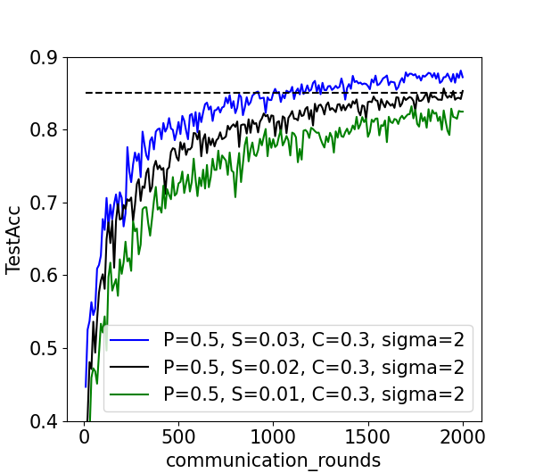
From Figure 2(c), Figure 2(d) and Figure 2(e), we can observe that as , and increase, the model performance and the convergence behavior are getting better. The phenomenon is quite reasonable because: 1) As aforementioned, the procedure of reconstructing distributions in H-FL is closely related to the training samples of each client. The larger and are, the more the training samples are, and the closer the reconstructed distribution is to the potential global distribution, thus reducing the impact of non-IID and obtaining a relatively ideal effect; 2) The number of training samples of each client has a great impact on noise injecting. As increase, the number of training samples of each client becomes larger, so that the in Formula 8 will be larger and the injected noise is correspondingly small; 3) As increases, the lossy compression becomes less and less effective and the behavior will get better. In addition, as the noise level increases in Figure 2(f), the oscillation amplitude of the accuracy curve becomes larger, the convergence speed becomes slower and the model performance becomes worse.
4.3 Effectiveness Of The Bias Corrector
Figure 3(a) shows the top-1 accuracy of VGG16 on CIFAR10 with and without the bias corrector. The black dotted line refers to an accuracy of 85%. As we can see, bias corrector has significant influence on the convergence behavior and the final accuracy of H-FL. When there exists the bias corrector, the accuracy of the global model converges to 85% around 1000 rounds. Whereas when we remove the bias corrector, the accuracy gradually approximates to 85% until 2000 rounds. Additionally, we take the average of the last 10 rounds of the accuracy as the final accuracy after 2000 rounds, and the bias corrector can achieve an improvement of 2.47 percentage points. The result of the experiment is in line with our expectation since the bias corrector gives a relatively precise approximation of when it can’t be calculated directly, and once we remove the bias corrector, it will obtain a biased , leading to the degradation in model performance and other metrics (convergence behavior).
4.4 Communication Overhead
Finally, we compare the different methods with respect to the communication overhead which are required to achieve a certain target accuracy. As we can see in the Figure 2(a) and Figure 2(b), the convergence behavior is much better than other methods, which considerably reduces the communication rounds. Notice that FedAVG does not converge on CIFAR10, thus we do not show that in Figure 3(c). To compare the communication overhead, we set a window of size 10, which is utilized to calculate an average of 10 rounds. The communication overhead accumulates while moving forward the window until the average accuracy is no less than the target accuracy (80% in our experiments). Figure 3(b) and Figure 3(c) show the communication overhead required to achieve the target accuracy for the different methods on FMNIST and CIFAR10 respectively.
5 Conclusion
In this paper, we present a Hierarchical Federated Learning architecture (H-FL) to find a great balance among model performance, communication overhead and privacy requirements. Firstly, we devise a runtime distribution reconstruction strategy to counter-weigh the degradation due to non-IID. Then we design a compression-correction mechanism to reduce the communication overhead without sacrificing the model performance. The experimental results have proved that H-FL achieves the state-of-the-art performance under different federated learning tasks.
Acknowledgements
We would like to thank anonymous reviewers for their helpful comments. This work was supported by the the National Key Research and Development Program of China (No. 2018AAA0100500), NSFC Grant No. 61872285, 62072367, 61772413, the Key Research and Development Program of Shaanxi Province (2020GY-033), Key Science and Technology Project of Henan Province (201300210400), Fundamental Research Funds for the Central Universities (xzy012020112).
References
- [Abadi et al., 2016] Martin Abadi, Andy Chu, Ian Goodfellow, H Brendan McMahan, Ilya Mironov, Kunal Talwar, and Li Zhang. Deep learning with differential privacy. In Proceedings of the 2016 ACM SIGSAC Conference on Computer and Communications Security, pages 308–318, 2016.
- [Kairouz et al., 2019] Peter Kairouz, H Brendan McMahan, Brendan Avent, Aurélien Bellet, Mehdi Bennis, Arjun Nitin Bhagoji, Keith Bonawitz, Zachary Charles, Graham Cormode, Rachel Cummings, et al. Advances and open problems in federated learning. arXiv preprint arXiv:1912.04977, 2019.
- [Konečnỳ et al., 2016] Jakub Konečnỳ, H Brendan McMahan, Felix X Yu, Peter Richtárik, Ananda Theertha Suresh, and Dave Bacon. Federated learning: Strategies for improving communication efficiency. arXiv preprint arXiv:1610.05492, 2016.
- [Krizhevsky et al., 2009] Alex Krizhevsky, Geoffrey Hinton, et al. Learning multiple layers of features from tiny images. Master’s thesis, University of Tront, 2009.
- [LeCun et al., 1998] Yann LeCun, Léon Bottou, Yoshua Bengio, and Patrick Haffner. Gradient-based learning applied to document recognition. Proceedings of the IEEE, 86(11):2278–2324, 1998.
- [Li et al., 2020] Tian Li, Anit Kumar Sahu, Ameet Talwalkar, and Virginia Smith. Federated learning: Challenges, methods, and future directions. IEEE Signal Processing Magazine, 37(3):50–60, 2020.
- [Lin et al., 2017] Yujun Lin, Song Han, Huizi Mao, Yu Wang, and William J Dally. Deep gradient compression: Reducing the communication bandwidth for distributed training. arXiv preprint arXiv:1712.01887, 2017.
- [Lin et al., 2018] Yujun Lin, Song Han, Huizi Mao, Yu Wang, and William J Dally. Deep Gradient Compression: Reducing the communication bandwidth for distributed training. In The International Conference on Learning Representations, 2018.
- [McMahan et al., 2017a] Brendan McMahan, Eider Moore, Daniel Ramage, Seth Hampson, and Blaise Aguera y Arcas. Communication-efficient learning of deep networks from decentralized data. In Artificial Intelligence and Statistics, pages 1273–1282. PMLR, 2017.
- [McMahan et al., 2017b] H Brendan McMahan, Daniel Ramage, Kunal Talwar, and Li Zhang. Learning differentially private recurrent language models. arXiv preprint arXiv:1710.06963, 2017.
- [Rothchild et al., 2020] Daniel Rothchild, Ashwinee Panda, Enayat Ullah, Nikita Ivkin, Ion Stoica, Vladimir Braverman, Joseph Gonzalez, and Raman Arora. Fetchsgd: Communication-efficient federated learning with sketching. In International Conference on Machine Learning, pages 8253–8265. PMLR, 2020.
- [Sattler et al., 2019] Felix Sattler, Simon Wiedemann, Klaus-Robert Müller, and Wojciech Samek. Robust and communication-efficient federated learning from non-iid data. IEEE transactions on neural networks and learning systems, 2019.
- [Simonyan and Zisserman, 2014] Karen Simonyan and Andrew Zisserman. Very deep convolutional networks for large-scale image recognition. arXiv preprint arXiv:1409.1556, 2014.
- [Vepakomma et al., 2018] Praneeth Vepakomma, Otkrist Gupta, Tristan Swedish, and Ramesh Raskar. Split learning for health: Distributed deep learning without sharing raw patient data. arXiv preprint arXiv:1812.00564, 2018.
- [Wei et al., 2020] Kang Wei, Jun Li, Ming Ding, Chuan Ma, Howard H Yang, Farhad Farokhi, Shi Jin, Tony QS Quek, and H Vincent Poor. Federated learning with differential privacy: Algorithms and performance analysis. IEEE Transactions on Information Forensics and Security, 2020.
- [Xiao et al., 2017] Han Xiao, Kashif Rasul, and Roland Vollgraf. Fashion-mnist: a novel image dataset for benchmarking machine learning algorithms. arXiv preprint arXiv:1708.07747, 2017.
- [Yang et al., 2019] Qiang Yang, Yang Liu, Tianjian Chen, and Yongxin Tong. Federated machine learning: Concept and applications. ACM Transactions on Intelligent Systems and Technology (TIST), 10(2):1–19, 2019.
- [Zhang et al., 2021] Qingsong Zhang, Bin Gu, Cheng Deng, and Heng Huang. Secure bilevel asynchronous vertical federated learning with backward updating. arXiv preprint arXiv:2103.00958, 2021.