Integer Coordinates for Intrinsic Geometry ProcessingJournal: TOGVolume: 99999999CCS: Mathematics of computing Mesh generation
Abstract.
In this work, we present a general, efficient, and provably robust representation for intrinsic triangulations. These triangulations have emerged as a powerful tool for robust geometry processing of surface meshes, taking a low-quality mesh and retriangulating it with high-quality intrinsic triangles. However, existing representations either support only edge flips, or do not offer a robust procedure to recover the common subdivision, that is, how the intrinsic triangulation sits along the original surface. To build a general-purpose robust structure, we extend the framework of normal coordinates, which have been deeply studied in topology, as well as the more recent idea of roundabouts from geometry processing, to support a variety of mesh processing operations like vertex insertions, edge splits, etc. The basic idea is to store an integer per mesh edge counting the number of times a curve crosses that edge. We show that this paradigm offers a highly effective representation for intrinsic triangulations with strong robustness guarantees. The resulting data structure is general and efficient, while offering a guarantee of always encoding a valid subdivision. Among other things, this allows us to generate a high-quality intrinsic Delaunay refinement of all manifold meshes in the challenging Thingi10k dataset for the first time. This enables a broad class of existing surface geometry algorithms to be applied out-of-the-box to low-quality triangulations.
Keywords:
remeshing, intrinsic triangulation, Delaunay triangulation, discrete differential geometry
1. Introduction and Related Work
Geometric data plays a growing role in applications from computational fabrication to to autonomous driving to augmented reality, but data in these applications is increasingly difficult to deal with due to the poor quality of meshes generated by non-expert users, or by algorithms targeted at visualization rather than mesh processing—there have hence been significant recent efforts to make geometric algorithms more robust [Zhou et al. 2016; Hu et al. 2018; Sellán et al. 2019; Sawhney and Crane 2020]. One basic tool is to remesh the input to obtain higher-quality elements, but for this approach to work on difficult, near-degerate inputs, remeshing algorithms must themselves be extremely robust. Moreover, traditional approaches to remeshing based on vertex positions in must negotiate the trade-off between mesh size, the quality of mesh elements, and geometric approximation of the input domain.
Intrinsic Triangulations.
A promising idea is to approach geometry processing from the intrinsic point of view: rather than considering the embedding of the geometry in space, one focuses only on point-to-point distances along the surface, as encoded by the edge lengths of a triangulation. This perspective is quite natural for problems in geometry processing and scientific computing, since many objects in these domains are themselves intrinsic—for instance, the Laplace-Beltrami operator, which appears in numerous algorithms and fundamental partial differential equations (PDEs). In this paper we consider so-called intrinsic triangulations, whose edges no longer need to be straight line segements in Euclidean space, but can instead be any straight or geodesic path across the input polyhedron (see Figure 2). This construction still captures the input geometry exactly, but provides a dramatically larger space of possible triangulations, lending enormous flexibility to geometric algorithms. For instance, it de-couples the quality of elements used for simulation from the elements used to describe the geometry, side-stepping the trade-off encountered in traditional meshing. Moreover, this perpective enables the input polyhedral surface to serve as a background domain—analogous to the Euclidean plane in traditional computational geometry—allowing one to “port” trusted algorithms from the plane to curved surfaces. Most importantly, by encapsulating all this machinery in an interface that resembles an ordinary mesh, one can provide robustness as a subroutine: rather than make existing algorithms more robust one by one, we can transform the input into an intrinsic triangulation, execute an ordinary (“non-robust”) algorithm, and then read off the reults in a variety of ways.
A remaining impediment to making the intrinsic approach truly reliable is to develop data structures for intrinsic triangulations that provide all the expected operations from standard mesh processing, while simultaneously providing strong guarantees of correctness. The basic challenge is encoding the correpsondence between the input mesh and an intrinsic triangulation sitting atop it, so that data on one triangulation can be transferred to the other. The first such data structure was the overlay mesh of Fisher et al. 2006. The overlay uses a halfedge mesh decorated with special vertex and edge attributes to maintain the common subdivision of and , i.e., the polygon mesh obtained by “slicing up” the underlying surface along the edges of both and . This approach guarantees correct connectivity, but ordinarily-local operations such as edge flips become non-local and expensive to evaluate—moreover, edge flips are the only operation supported by this data structure. Sharp et al. 2019a instead encode the correspondence implicitly by storing so-called signposts at vertices, which give the direction and length of each intrinsic edge. This approach is somewhat complementary to the overlay mesh: local mesh operations are now cheap to evaluate, but the encoding of connectivity now depends on floating-point values, and is hence not guaranteed to be correct. For instance, when tracing out intrinsic edges small floating point errors can cause one to “miss” the target vertex. A key development here, however, was extending intrinsic triangulations to operations beyond edge flips.

Integer-Based Encoding.
In this paper, we introduce an integer-based data structure for intrinsic triangulations that offers the best of both worlds: an implicit encoding of correspondence that supports fast local operations, but which is also guaranteed to correctly describe connectivity. Like the signposts, our data structure also supports a wide variety of local mesh operations (Section 3). As demonstrated in Section 5, we get dramatically improved robustness for difficult tasks, e.g., we achieve a 100% success rate for extracting a high-quality Delaunay refinement of low-quality input data. In turn, any algorithm that relies on a high-quality triangulation (e.g., for solving PDEs) can immediately benefit from this improved robustness. For instance, in Section 4 we observe improved robustness for computing geodesic distance, local parameterization, constructing geodesics, and finding smooth vector fields.
The basic starting point for our data structure is the concept of normal coordinates from geometric topology (not to be confused with geodesic normal coordinates from Riemannian geometry). However, we must augment this construction in several ways in order to make it suitable for geometry processing. As detailed in Section 2.3, the basic idea of normal coordinates is to simply count how many times each edge of a triangulation is crossed by some curve (Figure 3). Such coordinates were originally developed to study not curves, but rather embeddings of surfaces in 3-manifolds [Kneser 1929; Haken 1961; Hass and Trnkova 2020], and subsequently appear in several places in mathematics (e.g., for studying the mapping class group [Farb and Margalit 2011]), including significant work on algorithms [Bell 2015; Bell 2018; Schaefer et al. 2008]. In theoretical computer science, normal coordinates are also viewed as a means of “compressing” curves, e.g., the total number of bits required to store a long winding curve can be exponentially smaller than storing explicit segments along the curve [Erickson and Nayyeri 2013].
One challenge with using normal coordinates for geometry processing is that existing literature rarely considers operations beyond edge flips: the little that does considers only closed loops e.g. [Schaefer et al. 2002, Section 5.4], whereas curves that terminate at vertices are absolutely essential for encoding triangulations. A second issue is that normal coordinates alone are not enough to uniquely identify curves implied by the coordinates with logical edges of a mesh. Very recently, Gillespie et al. 2021 proposed a solution to this issue using what they call roundabouts, but again do not consider operations beyond edge flips. Third, whereas most literature assumes that normal coordinates encode homotopy classes of curves in a purely topological setting (or perhaps hyperbolic geodesics), we must make a significant departure this perspective and assume that the normal coordinates encode a triangulation of a Euclidean polyhedron by geodesic edges. This distinction is important since, in general, not all normal coordinates describe a valid Euclidean geodesic triangulation. Considering this special case in turn enables us to establish procedures not previously seen.
Contributions.
Overall, we make the following contributions:
- •
We describe normal coordinates as a representation for general intrinsic triangulations, including the case where vertices have been added to the triangulation.
- •
We extend integer-based data structures for geometric intrinsic triangulations to include local operations beyond edge flips.
- •
We prove the correctness and quality of a Delaunay refinement algorithm for intrinsic triangulations of surfaces without boundary.
- •
We also extend intrinsic Delaunay refinement to surfaces with boundary.
- •
We introduce a new, more accurate way of transferring functions between bases on different triangulations.
We also experimentally validate the robustness of our technique, including generating intrinsic Delaunay refinements for all manifold meshes in the Thingi10k dataset, and demonstrate robustness for a variety of basic algorithms from geometry processing.
2. Notation and Conventions
2.1. Connectivity
Throughout we assume that our domain is an oriented manifold surface , possibly with boundary. We write to denote a triangulation of with vertices , edges , and faces . In general we allow triangulations that are not be simplicial, but can instead be a -complex in the sense of Hatcher 2002—we allow, e.g., two edges of the same triangle to be glued together (see inset). We will refer to vertices , edges , and faces by one, two, or three indices, resp.. Note that as our triangulations need not be simplicial, the vertices of an edge may not be distinct, and do not necessarily identify the edge—there may be multiple edges between and .
We will refer to oriented halfedges , and will use to denote a value at corner of triangle , and to denote a value at halfedge . Throughout, we consider a fixed input triangulation of , as well as a dynamic intrinsic triangulation sitting atop . must contain all vertices of , i.e. , but may include additional inserted vertices which we denote by . We will generally use indices for vertices of and indices for vertices of (which may also be in ).
2.2. Geometry
The geometry of a triangulation is determined by a collection of edge lengths satisfying the triangle inequalities in each face. For instance, we typically begin by assigning and the same edge lengths determined by vertex coordinates . While the lengths remain fixed, the edge lengths of may change due to operations like intrinsic edge flips (Section 3.3). Even after changing the edge lengths, each individual triangle can always be drawn as an ordinary triangle in the Euclidean plane, allowing us to compute quantities such as face areas or corner angles. In general, we will not need to simultaneously embed all triangles of in . Finally, we use
to denote the exponential map at . Given a tangent vector at , is the point reached by walking straight along the surface in the direction of for a distance (see inset). (In practice this can be implemented as in [Sharp et al. 2019a, Section 3.2.2]).
Points can be expressed in barycentric coordinates relative to some simplex (vertex, edge, or triangle) of a triangulation , e.g., a point in a triangle is given by three coordinates such that . For vertices, we set the single coordinate to 1. Importantly, we will need to encode points with respect to two different triangulations and , using barycentric coordinates and , resp. (Figure 4). Note that for vertices that are shared by both triangulations, we have . We will use to denote a location on represented by simplex along with a barycentric coordinate, and similarly will use for a location on .

2.3. Integer Coordinates
Normal coordinates.
We use normal coordinates to count the number times each edge of crosses the edges of (see Figure 5, left). In principle, normal coordinates could either be defined as a value per edge of , counting the number of crossings from , or as a value per edge of . In our setting, we take the latter approach, as it remains fully-informative even when we insert new vertices in to . It is then natural to think of as the primary triangulation, with as a collection of geodesic curves sitting along it (Figure 5, right). To emphasize this abstract viewpoint, we will refer to the edges of as curves. Because we allow edges to be split, a single edge may actually correspond to a sequence of curves expressed in normal coordinates which meet at intermediate vertices .
Precisely, we use to denote the normal coordinates. For each edge , the quantity indicates how many times is crossed by edges of : if , then this is a count of crossings (formally, transversal intersections), whereas if , it indicates that a curve runs along edge (Figure 5, left). Note that is never less than because we are working with triangulations, and multiple edges of a triangulation cannot lie along the exact same path. We use to denote the number of transversal crossings, i.e. , and similarly define , which is 1 on shared edges and 0 otherwise.
Additionally, we define two quantities at each corner of , which count how many curves emanate from the interior of the corner and cross the corner resp. (Figure 6):
| (1) | ||||
| (2) |
Crossings.
A point where a curve crosses an edge can be described either in a combinatorial or geometric sense. A combinatorial crossing is given by a pair , such that is the crossing along oriented edge . A geometric crossing is similarly given by , where encode the location of the crossing along the curve and along the (resp.) in barycentric coordinates. Importantly, both of these crossings are oriented: the choice of halfedge versus indicates which side of the edge one is “coming from” and “going to,” which will be important when tracing out curves along the surface. We let denote a reversal of orientation.
Roundabouts
Normal coordinates alone do not fully encode the correspondence between and , because we cannot necessarily determine which curve along corresponds to which edge of (recall that there may be multiple edges of between the same pair of vertices). Thus we additionally store roundabouts , introduced by Gillespie et al. 2021, which describe how the edges of and are interleaved around vertices. Unlike Gillespie et al., we may insert new vertices—however, we still store roundabouts only at halfedges pointing away from shared vertices . These are sufficient to disambiguate the identity of any traced curve, since all edges of must start and end at vertices in (if an edge has been split, then the sequence of curves starts and ends at vertices in ).
Precisely, for each halfedge starting at a shared vertex , the roundabout stores the first halfedge following . This is encoded as an index , where we enumerate the halfedges of about vertex in counterclockwise order (Figure 7)
3. Algorithms and Data Structures
In this section, we provide descriptions of our data structure and the operations that it supports. Detailed pseudocode can be found in Appendix A.
3.1. Data Structure
The most essential data to maintain is a mesh of triangulation ; recall that . We use a halfedge mesh, since halfedge meshes can represent general -complexes (Section 2.1), though one could also use a vertex-face adjacency list plus a small amount of additional data [Sharp and Crane 2020a, Section 4.1]. On top of this mesh, our data structure maintains four quantities:
- •
lengths for each edge ,
- •
normal coordinates for each edge ,
- •
roundabouts for each halfedge incident on a vertex shared with ,
- •
barycentric coordinates relative to for each .
This differs from the scheme of Gillespie et al. 2021 in a few key ways. The essential difference is that their data structure assumes that and share the same vertex set (). This has numerous consequences—e.g. they use nonnegative normal coordinates , they do not store input positions . Most importantly, it is impossible to perform many of the local mesh operations we describe in the next section without changing the vertex set of ; our generalization of the representation is essential if one wants to perform tasks such as Delaunay refinement (Section 4.2).
3.2. Extracting Curves
Our first task is to recover a curve on from its normal coordinates—because our curves are geodesic, we can determine the exact geometry from these normal coordinates. In particular, we describe a procedure ExtractCurve (Algorithm A) which takes in any combinatorial crossing along a curve, and computes the curve’s trajectory along as a sequence of geometric crossings along with start and end vertices . We note that this mirrors the discussion in Gillespie et al. 2021, albeit in a more general setting; we include a full description here for completeness.
We proceed in two steps, first determining the triangle strip that the curve passes through and only then computing the curve’s geometry. Note that the triangle strip depends solely on the integer-valued normal coordinates , while geometric data and floating point computation are relegated to the second step.
The first step is performed by TraceFrom (Algorithm A), which takes some combinatorial crossing along a curve , and traces out the remaining combinatorial crossings until terminates at a vertex. TraceFrom proceeds iteratively, taking the crossing where enters a triangle, and using the triangle’s normal coordinates to determine where exits (see Figure 8). The direction in which to trace the curve is determined by the orientation of .
To determine the triangle strip containing , ExtractCurve calls TraceFrom once in either direction, yielding the sequence of all combinatorial crossings along . ExtractCurve then unfolds this triangle strip in an arbitrary planar coordinate system and draws as a straight line between its endpoints. The intersection of this line with each of the intermediate edges determines the geometric crossings along (Figure 9). Note that unlike Gillespie et al. 2021, we may have to invoke ExtractCurve multiple times to extract a single edge , as it may pass through several vertices of , e.g. due to edge splits (Section 3.5).
Finally, it is sometimes useful to convert a single combinatorial crossing into a geometric crossing . We will refer to this operation as ExtractGeometricCrossing; it may be implemented by calling ExtractCurve and then returning the single desired crossing.

3.3. Edge Flip
Edge flips are a well-studied operation, but we include a discussion here for completeness. We may flip and edge if and only if (i) both endpoints have degree at least one after the flip, and (ii) the two triangles containing the edge form a convex quadrilateral (Figure 10).
Mesh Update
We replace edge with an edge . We compute the new edge length by laying out the two old triangles in the plane and measuring the length of the appropriate diagonal.
Normal Coordinates & Roundabouts
The new normal coordinate does not depend at all on the geometry of . It is given by the following formula:
| (3) | ||||
This differs slightly from the formula of Gillespie et al. 2021, which did not allow for inserted vertices.
We can update each roundabout from its previous neighbor:
| (4) |
where is the degree of vertex in triangulation . The quantity counts how many edges of are between and : counts edges strictly between them, and adds one if there is also an edge lying exactly along .
We only perform this update for halfedges whose source is in .
3.4. Face Split
We now describe procedure SplitFace ( Algorithms A and A), the first of several new routines to mutate triangulation while tracking the correspondence with . Note that Schaefer et al. 2002 describe a similar face split operation in the topological setting, but do not provide the ability to insert a point at a particular geometric location, which is essential in our setting of Euclidean polyhedra.
In particular, suppose we wish to insert a vertex at a point , given by barycentric coordinates on a triangle . To do so, we need to update the connectivity , edge lengths , normal coordinates , and roundabouts . Additionally, we need to compute the position of this new vertex in barycentric coordinates on .
Mesh Update
We update the connectivity of with a new vertex and three new edges and faces. We compute new edge lengths as a formula of the barycentric coordinates . Schindler and Chen 2012 show that the length of a displacement vector in barycentric coordinates is give by
| (5) |
Normal Coordinates & Roundabouts
Unlike the case of an edge flip, where the new normal coordinate depends solely on the initial normal coordinates, vertex insertion is an inherently geometric operation. Different points necessarily result in different normal coordinates (see inset), depending on the region in which the point lies.
Concretely, we first compute the geometric crossings of all curves passing through face (using the ExtractGeometricCrossing subroutine). We then determine which region the new point lies in via a series of line-side tests. (One might in principle be able to reduce the number of curves that need to be extracted via lazy evaluation or caching, though we do not pursue such optimizations here.) We may misclassify points extremely close to a region’s boundary due to floating point error, in which case we insert a valid point in the identified region, at a virtually identical location. Note that this behavior is perfectly reasonable in, e.g., retriangulation algorithms (see Section 4.2), where the insertion location is not computed exactly anyway.
The roundabouts on any new halfedges emanating from original vertices (i.e., vertices in ) can be set from their neighbors via Equation 4.
Position on
To determine , we must locate the triangle containing , as well as the barycentric coordinates of within . We do so via interpolation from the corners of . Explicitly, the corners of are all geometric crossings with known barycentric coordinates in some triangle (computed in ExtractGeometricCrossing); we can then solve a small linear system to recover the barycentric coordinates of in the same triangle. Intuitively, we recover generalized barycentric coordinates for with respect to the polygon and apply them on to recover standard barycentric coordinates in (see Appendix B for details).
3.5. Edge Split

We also introduce an operation SplitEdge (Algorithm A), which takes as input a point given by barycentric coordinates along an oriented edge . If does not have a curve running along it (i.e. ), then this is implemented as a face split followed by an edge flip (Figure 11, top). However, if (which is common in practice—e.g. Section 4.2), we perform an explicit edge split which inserts the new vertex along the coincident curve (Figure 11, bottom).
Mesh Update
We insert a new vertex and triangulate any adjacent faces, computing the new edge lengths via Equation 5.
Normal Coordinates & Roundabouts
When the new normal coordinates are simple functions of the old ones, since every curve in face must emanate from or , or cross . The number of such curves is and edge crosses them all. We hence set and equal to , and set
| (6) |
As with face splits, roundabouts on any new halfedges emanating from original vertices can be set from their neighbors (Equation 4).
Position on
To determine , we must locate the edge containing , as well as the barycentric coordinates of within . Since, and necessarily have known locations along some edge in , we can simply interpolate by to compute the location .
3.6. Vertex Removal
In general, a vertex which is present in the original triangulation cannot be removed without distorting the intrinsic metric because any curvature at that vertex would be lost. However, inserted vertices have no curvature, and can hence be removed safely. In fact this operation will be necessary for Delaunay refinement of domains with boundary (Section 4.2).
The basic strategy behind RemoveVertex (Algorithm A) is to flip edges incident on the vertex to be removed until it has degree three, then delete the three edges incident on the vertex as well as the vertex itself. No other data needs to be updated, since the edges of the resulting triangle already appear in the triangulation. Algorithm A describes this procedure, and Theorem D.1 proves its correctness for simplicial complexes. A nearly identical procedure can be used to remove an inserted boundary vertex. Schaefer et al. 2002 also suggest a similar flipping procedure, but work in the topological setting where the necessary edge flips are always valid—they do not consider the convexity condition (Section 3.3).
3.7. Moving Inserted Vertices
Given the previous operations, we can easily define a procedure for moving around inserted vertices. Specifically, given a vector in the tangent space of an inserted vertex , we can move along in the following way:
- •
First, compute the new location .
- •
Insert using SplitFace.
- •
Remove using RemoveVertex.
We insert first since the removal procedure could flip edges incident on the triangle containing , invalidating its barycentric coordinates. Note that Sharp et al. propose an alternative strategy for local vertex displacement [Sharp et al. 2019a, Section 3.3.3].
3.8. Common Subdivision
As noted previously, the common subdivision of and is the polygon mesh obtained by “slicing up” the underlying surface along the edges of both and . The vertices of are hence a superset of and , and every edge or face of and can be expressed as union of edges or faces of (resp.). Moreover, the faces of are always planar and convex. Most importantly in our setting, any piecewise-linear function on or can be represented exactly as a piecewise-linear function on . Note however that even if and have nice elements, is not in general a high-quality mesh, and may not itself be suitable for, e.g., solving PDEs. Rather, it plays a complementary role in the geometry processing pipeline, enabling (for instance) transfer of data between triangulations (Section 4.4), or visualization of data downstream via standard rendering tools.
We compute the common subdivision by cutting along the edges of . First we extract the connectivity of , using only the normal coordinates . Then we recover the intersection geometry, allowing us to interpolate data stored at the vertices of or to —most commonly, vertex positions on along with any solution data on . Note that this procedure was previously described by Sharp et al. 2019a; we recap it here for completeness, and to give a convenient description using our integer coordinates.
Connectivity.
We subdivide independently in each face . The normal coordinates alone determine the connectivity of within this face. There are just two cases to consider, illustrated in Figure 12. Case 1 occurs when no curves emanate from any corner, so we simply need to connect the first crossings along edge to the first crossings along (in order), and likewise for corners and . In Case 2 curves emanate from some corner; without loss of generality, let this corner be so that the number of such curves is and there are more curves crossing edge than the other two edges. Hence, we can walk from to , connecting the first crossings to those along , the next crossings to vertex , and the remaining crossings to those along edge . Note that curves running along edges () require no special treatment.
Intersection Geometry.
Next, we associate each vertex of the common subdivision with a point in and a point in , encoded in barycentric coordinates relative to some simplex (vertex, edge, or face) of the appropriate triangulation. Using this, one can linearly interpolate data in the usual way. Again, there are just two cases: each vertex in is either a vertex of or the intersection of an edge of with an edge of . In the first case, the position on is given by itself, and its position on was computed when was inserted. In the second case, we compute the desired barycentric coordinates using ExtractCurve (see Algorithm A for details).
3.9. Transposing Coordinates
Throughout, we store normal coordinates which count how many times edges of cross edges of . It is sometimes useful to observe that tracing an edge over counts how many times crosses edges of . If has more vertices than , then the edges of are not normal over —they can start and end in the middle of faces of —and these crossing counts do not uniquely encode the structure of . However, if and do have the same vertex set, then these crossing counts provide an implicit representation of as a collection of curves over .
3.10. Visualization
In the following, we show examples of intrinsic triangulations on top of meshes (e.g. Figure 13). To produce these figures, we compute the common subdivision (Section 3.8) and draw the edges of the input mesh with a black wireframe while coloring the intrinsic triangles in arbitrarily-chosen colors. In figures displaying functions defined on intrinsic triangulations (e.g. Figure 15), we interpolate the solutions along the common subdivision for rendering.
3.11. Robust Implementation
Our integer coordinates are guaranteed to encode a triangulation sitting atop . The geometric accuracy of this triangulation, of course, depends on floating point arithmetic, which can become inaccurate in near-degenerate configurations. Exact predicates have been applied with great success to similar problems [Devillers and Pion 2003]. Unfortunately they do not directly apply to intrinsic triangulations, as the predicates that we evaluate are not fixed functions of the input data; an intrinsic edge length can depend upon arbitrarily many input edge lengths. Hence, we focus on fast and robust implementations using ordinary floating point arithmetic.
One essential tool for dealing with intrinsic triangulations on near-degenerate input meshes is intrinsic mollification, introduced by Sharp and Crane 2020a. Mollification improves degenerate meshes by adding a small to every edge length, provably improving triangle quality. This changes the geometry by a negligible amount, and moreover we only mollify if some triangle is within of being degenerate. This procedure works particularly well with our data structure compared to signposts: the signpost data structure relies on tracing queries along the surface which become less accurate when mollification is applied. Our integer coordinates have no such problem: we always get the correct edge sequence, even if the mesh geometry is slightly modified. In our experiments we mollify with , and find that it resolves almost all numerical difficulties.
Even after mollification, it is still beneficial to use care when working with floating point. For example, there are well-conditioned triangles on which the Delaunay condition (Equation 8, discussed in the next section) is difficult to evaluate; in practice, we only enforce Equation 8 up to some tolerance. As a further example, when computing new normal coordinates in SplitFace, one could lay out the face in the plane, and independently count intersections along the new edges. However, this can produce invalid normal coordinates in floating point. We apply a more complicated policy (see Appendix A) which always yields valid normal coordinates. For additional details on all procedures, we refer the reader to our implementation, which will be made available after review.
3.12. Other Algorithms
Normal coordinates also enable a wide variety of other operations not detailed here. For instance, Schaefer et al. 2002 provide algorithms for counting connected components, checking if crossings are part of the same curve, checking if curves are isotopic, and computing the oriented intersection number. Erickson and Nayyeri 2013 provide an asymptotically-fast algorithm for tracing normal curves across a surface. Finally, Dynnikov 2020 provides an algorithm for computing how many times curves represented by normal coordinates intersect.
4. Applications
4.1. Intrinsic Delaunay Triangulations

One key application of intrinsic triangulations is the computation of intrinsic Delaunay triangulations (Figure 13, top). A triangulation is said to be Delaunay if the sum of angles opposite every edge is at most , i.e. for every we have
| (7) |
Delaunay triangulation have a number of beneficial properties. One consequence of Equation 7 is that edges of a Delaunay triangulation must have nonnegative cotan weights:
| (8) |
In fact, Equation 8 is equivalent to Equation 7 above, and provides a convenient formula for checking the Delaunay property in an intrinsic triangulation. Moreover, Equation 8 ensures that the finite element Laplacian satisfies the maximum principle, guaranteeing that discrete harmonic functions do not have local extrema in the interior of the domain [Bobenko and Springborn 2007, Proposition 19]. Similarly Equation 8 also ensures that discrete harmonic vector fields are “flip-free” [Sharp et al. 2019b, Section 5.4]. Furthermore, the local Delaunay condition implies the empty circumcircle property: each triangle’s geodesic circumdisk contains no vertices, illustrated in Figure 14, left [Bobenko and Springborn 2007, Proposition 10].
The Delaunay triangulation can be computed via a simple greedy algorithm: flip any non-Delaunay edge until all edges satisfy Equation 7 [Bobenko and Springborn 2007, Propositions 11 and 12].
4.2. Intrinsic Delaunay Refinement
Delaunay refinement inserts vertices in order to produce a Delaunay mesh whose triangles all satisfy a minimum angle bound (Figure 13, bottom). Here we modify Chew’s second algorithm to perform intrinsic Delaunay refinement [Chew 1993; Shewchuk 1997]. This problem has been extensively studied in the plane, but an intrinsic (i.e. geodesic) scheme was only recently proposed by Sharp et al. 2019a. However, they did not handle meshes with boundary—here we resolve the essential difficulties of the boundary case, and show how refinement can be implemented using our integer-based data structure.
In the plane, the basic algorithm is to greedily pick any triangle which violates the minimum angle bound, insert a vertex at its circumcenter, then flip to Delaunay. This process continues until all triangles satisfy the angle bound. If a triangle’s circumcenter is outside the domain, then the boundary edge separating the triangle from its circumcenter is split at its midpoint; subsequently, all interior vertices within at least a distance of are removed—though removing additional interior vertices causes no issues (Appendix C.1). One can prove that this process succeeds for minimum angle bounds up to 25.65 degrees on planar domains with boundary angles at least [Shewchuk 1997, Section 3.4.2]. More advanced versions of this procedure can achieve better angle bounds, e.g. [Rand 2011], but here we restrict our attention to the basic algorithm for simplicity.
There are two difficulties in adapting this algorithm to the intrinsic setting: locating circumcenters and computing (geodesic) distances. As mentioned earlier, intrinsic Delaunay triangulations obey the empty circumcircle property; hence each triangle has an intrinsically-flat circumdisk with a well-defined center (Figure 14, left). So long as this center corresponds to a point on the surface, it can be found by walking from the triangle’s barycenter (Figure 14, right). In practice, we compute triangle ’s circumcenter in homogeneous (i.e., unnormalized) barycentric coordinates via the following formula [Schindler and Chen 2012, Section 2.3]:
| (9) |
and then normalize to obtain barycentric coordinates
| (10) |
To locate the circumcenter on the surface, we then evaluate the exponential map (Section 2.2) starting at the barycenter , along the vector . If we hit a boundary edge while tracing out this path, then the circumcenter is not contained in the surface, so we split at its midpoint and flip to Delaunay. We must then remove all inserted interior vertices within a geodesic ball of radius centered at the inserted point. Computing geodesic distance on a surface mesh is nontrivial, but Xia 2013 shows that on a Delaunay triangulation any vertex inside a geodesic ball of radius will also be inside the Dijkstra ball of radius (i.e. points whose distance along the edge graph are at most ). We hence remove all interior inserted vertices within a Dijkstra distance of . Note that while Xia considers only the planar setting, their proof (which is based on triangle strips) applies without modification to intrinsic Delaunay triangulations of surfaces.
On meshes with narrow cone vertices or boundary angles, it may be impossible to find any triangulation satisfying a given angle bound. In such cases, we do not insert circumcenters of intrinsic triangles which are incident on exactly one narrow vertex, or are entirely contained in a triangle of which is incident a narrow vertex, and ignore such triangles when computing the minimum corner angle of the output mesh. Although the final output may violate the angle bound, such triangles appear only near narrow vertices. In analogy with the planar case, we set as the minimum allowed angle sum (see inset); in practice the vast majority of meshes obey this constraint at all vertices (97.2% of Thingi10k), and even on those which do not we obtain high-quality triangulations.
4.3. PDE-Based Geometry Processing

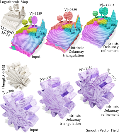
PDE-based methods abound in geometry processing, as they are generally simple to implement and benefit from decades of research into linear solvers, Many such methods depend only on intrinsic data, and are hence a natural application of our intrinsic Delaunay triangulations and refinements. On near-degenerate inputs, simply running the standard algorithm on an intrinsic triangulation instead of the original mesh yields solutions of dramatically higher quality ( Figures 15 and 16).
We show several examples: fast geodesic distance computation [Crane et al. 2017], local parameterization via the logarithmic map [Sharp et al. 2019b], and smooth vector fields [Knöppel et al. 2013]. Further examples on tasks such as parameterization, minimal surfaces, and surface editing can be found in [Sharp et al. 2019a; Sharp and Crane 2020a]. Across the board, normal coordinates offer improved robustness guarantees, and open doors to higher solution accuracy with the common subdivision.
4.4. Attribute Transfer

Intrinsic triangulations can drastically improve the quality of solutions to PDEs on low-quality meshes. However in practice, one often needs to represent the solution on the input mesh. Past approaches have simply “copied back” the solution values at vertices of the original mesh, but this strategy is ad-hoc and suboptimal. A more principled approach is to choose the function on the original mesh which is closest to the intrinsic solution. Here, we restrict our treatment to piecewise-linear bases and distance for simplicity, though the same strategy could easily be applied to other basis functions and notions of distance. Precisely, given a function on the intrinsic triangulation, we seek on the original mesh that minimizes the squared distance
| (11) |
Here, and are functions represented in finite-dimensional bases with nodal values at the vertices of the intrinsic triangulation and the original mesh resp. In traditional finite elements, this integral commonly arises over a single triangulation, in which case it can be evaluated via the Galerkin mass matrx as
| (12) |
where is constructed as in [Strang and Fix 2008, Chapter 10, (32)]. However, in our setting and are encoded over different triangulations; they are members of different function spaces. Our key observation is that the common subdivision (Section 3.8) provides exactly the structure needed to evaluate , as both functions are linear on each triangle of . In fact, we have
| (13) |
where now is the Galerkin mass matrix of the common subdivision, and are interpolation matrices which map piecewise-linear functions on original and intrinsic triangulations to piecewise-linear functions on , resp. In particular, is a matrix, where each row corresponds to a vertex of , and has that vertex’s barycentric coordinates on as entries. is defined likewise for . We then find the function which minimizes Equation 13 as the solution to a linear least-squares system, which can be prefactored if desired to efficiently transfer many functions.
We can leverage this formulation to transfer functions from any intrinsic triangulation back to the original mesh. In Figure 17, we show how this transfer indeed improves the accuracy of PDE solutions as measured on the original low-quality mesh. This machinery is enabled because our integer coordinates efficiently and robustly compute the common subdivision. More broadly, this paradigm opens the door to a wide variety of future finite-element formulations involving intrinsic triangulations.
4.5. Flip-Based Geodesic Paths

The previous sections have demonstrated the value of intrinsic triangulations as a high-quality basis for discretizing functions on surfaces; more broadly, these triangulations also provide simple and robust solutions to other tasks across geometry processing. As an example, the recent FlipOut procedure of Sharp and Crane 2020b computes exact geodesic paths on surfaces via a simple intrinsic edge flipping strategy, introducing the geodesic as a path of edges in the triangulation. This method is easily implemented in our integer representation in terms of the mesh operations in Section 3, and the resulting geodesic paths may then be recovered with the ExtractEdge subroutine. Computing geodesics with our robust integer coordinates is particularly appealing, because geodesic algorithms are notoriously difficult to implement robustly [Sharp and Crane 2020b, Section 5.3]. Even the method of Sharp et al. uses the signpost data structure, which may fail to reconstruct a connected path along the surface for degenerate inputs. In contrast, implementing FlipOut in our integer coordinate representation extends the benefits of our approach to this task, including a guarantee of valid connectivity in the output (Figure 18, left). It also enables higher-level tasks involving geodesic paths to be safely run on low-quality input, such constructing geodesic loops on surfaces, and even geodesic Bézier curves, using a de Casteljau-style scheme due to Morera et al. 2008 as shown in Figure 18, right.
5. Evaluation
| Method | Intrinsic Delaunay Triangulation | Intrinsic Delaunay Refinement |
|---|---|---|
| Explicit Overlay | 100 % | - |
| Signpost Tracing | 96.0 % | 69.1 % |
| Integer Coordinates | 100 % | 100 % |
We implemented all algorithms in C++; since basic vertex-face adjacency list cannot represent a general -complex (Section 2.1), we use a halfedge data structure for triangle meshes. Timings are measured on a single core of an Intel i9-9980XE with 32 GB of RAM.
Performance
Generally our data structure is quite fast, computing Delaunay refinements for complex meshes in seconds. For example, computing the Delaunay refinement Figure 15 takes 0.2s, and the Delaunay refinement in Figure 16 (top) takes 0.6s. Because we lazily recover intersection geometry from our integer coordinates when inserting vertices, routines such as Delaunay refinement which perform many insertions may become moderately expensive on large near-degenerate inputs. For instance we take 4 minutes to perform Delaunay refinement on 719791 (Figure 20, top) which signposts does in 1.5 minutes, but on such meshes signposts generally fails to compute a valid common subdivision at the end. Section 6 discusses hybrid routines which may give the best of both worlds.
5.1. Robustness

We validate robustness by successfully computing Delaunay triangulations, refinements, and their common subdivisions on all manifold meshes in Thingi10k [Zhou and Jacobson 2016]. In particular, we used MeshLab to convert each mesh to the PLY file format [Cignoni et al. 2008], resulting in 7696 valid manifold meshes. We begin by mollifying each mesh to a tolerance of (Section 3.11). For each model we compute the intrinsic Delaunay triangulation (Section 4.1) with a tolerance of , as well as an intrinsic Delaunay refinement (Section 4.2) with a angle bound. We verify that the algorithms terminate with the expected conditions. Additionally, we successfully extract an explicit mesh of the common subdivision in both cases, except for 1 model in the case of refinement whose common subdivision contains around 30 million vertices (Figure 20, top).
We compare against the explicit overlay representation of Fisher et al. 2006 and the signpost representation of Sharp et al. 2019a (Table 1). The overlay representation similarly offers a guarantee of valid connectivity, but does not provide a constant-time edge flip operation (like normal coordinates do). More importantly it does not support operations beyond edge flips and thus cannot perform Delaunay refinement. Signposts support a wide range of operations, but may not successfully recover the common subdivision on degenerate inputs (Figure 19). The statistic reported here differs from the result in Sharp et al. 2019a, because no preprocessing of meshes is performed. For refinement Sharp et al. 2019a do not treat the boundary case, so we evaluate only on models without boundary.

6. Limitations and Future Work
Limitations
The common subdivisions that we compute after Delaunay refinement can be quite large: the mean increase in is , and the percentile increase is . We emphasize again that the common subdivision is not generally a high-quality mesh anyway: one should perform numerical computations on the intrinsic triangulation instead. The intrinsic mesh has much higher element quality and is generally much smaller with a mean increase in of and percentile increase of . However, for applications that rely on the common subdivision (e.g. Section 4.4), it would still be beneficial to explore strategies for simplifying .
A related issue is that Delaunay refinement sometimes generates meshes with many small triangles. One can prove that Delaunay refinement in the plane produces well-graded meshes, meaning essentially that it only places small triangles in regions with small features, and our Delaunay refinement on surfaces seems to behave similarly. Nonetheless, on poorly-conditioned input meshes, Delaunay refinement can insert many small triangles. This can cause problems for diffusion-based algorithms (e.g. the logarithmic map computation in Figure 16), which use the mean edge length to determine a suitable diffusion time. We found that computing the diffusion time on the original mesh and then performing diffusion on the intrinsic triangulation produced the best results.
Hybrid Data Structures
At this point, there are several intrinsic triangulation data structures, but no single one is perfect:
- •
Overlay (explicit) provides exact connectivity; flipping can be slow; no vertex insertion.
- •
Signposts (implicit) provide inexact connectivity; flipping and vertex insertion are both fast.
- •
Integer coordinates (implicit) provide exact connectivity; flipping is fast; vertex insertion can be slow.
We propose a good way to get the best of all worlds would be to use a hybrid signpost + integer coordinate data structure. This is fully implicit, so you don’t pay the cost when you have edges crossing edges. But, flipping and insertion are both fast, and connectivity is exact, if you accept the inserted locations.
Even further in the implicit direction, storing edge lengths is an “optimization” in our data structure. One could just store the normal coordinates and original triangulation, recovering edge length whenever necessary via a layout operation. This is appealing, since it is truly an integer-only representation for intrinsic triangulations.
General geodesic curves
It would also be natural to use this machinery as a representation for general geodesic curves on surfaces, which commonly arise in geometry processing tasks such as cutting, segmentation, etc..
7. Acknowledgments
This work was supported by a Packard Fellowship, NSF Award 1717320, DFG TRR 109, an NSF Graduate Research Fellowship, and gifts from Autodesk, Adobe, and Facebook.
References
- [1]
- Bell [2018] Mark Bell. 2013–2018. flipper (Computer Software). pypi.python.org/pypi/flipper.
- Bell [2015] Mark Bell. 2015. Recognising mapping classes. Ph.D. Dissertation. University of Warwick.
- Bobenko and Springborn [2007] Alexander I Bobenko and Boris A Springborn. 2007. A discrete Laplace–Beltrami operator for simplicial surfaces. Discrete & Computational Geometry 38, 4 (2007), 740–756.
- Chew [1993] L Paul Chew. 1993. Guaranteed-quality mesh generation for curved surfaces. In Proceedings of the ninth annual symposium on Computational geometry. 274–280.
- Cignoni et al. [2008] Paolo Cignoni, Marco Callieri, Massimiliano Corsini, Matteo Dellepiane, Fabio Ganovelli, and Guido Ranzuglia. 2008. Meshlab: an open-source mesh processing tool.. In Eurographics Italian chapter conference, Vol. 2008. Salerno, Italy, 129–136.
- Crane et al. [2017] Keenan Crane, Clarisse Weischedel, and Max Wardetzky. 2017. The Heat Method for Distance Computation. Commun. ACM 60, 11 (Oct. 2017), 90–99.
- Devillers and Pion [2003] Olivier Devillers and Sylvain Pion. 2003. Efficient Exact Geometric Predicates for Delauny Triangulations.. In Proc. 5th Workshop Algorithm Eng. Exper. 37–44.
- Dynnikov [2020] Ivan Dynnikov. 2020. Counting intersections of normal curves. arXiv preprint arXiv:2010.01638 (2020).
- Erickson and Nayyeri [2013] Jeff Erickson and Amir Nayyeri. 2013. Tracing compressed curves in triangulated surfaces. Discrete & Computational Geometry 49, 4 (2013), 823–863.
- Farb and Margalit [2011] Benson Farb and Dan Margalit. 2011. A primer on mapping class groups (pms-49). Princeton University Press.
- Fisher et al. [2006] Matthew Fisher, Boris Springborn, Alexander I Bobenko, and Peter Schroder. 2006. An algorithm for the construction of intrinsic Delaunay triangulations with applications to digital geometry processing. In ACM SIGGRAPH 2006. 69–74.
- Gillespie et al. [2021] Mark Gillespie, Boris Springborn, and Keenan Crane. 2021. Discrete Conformal Equivalence of Polyhedral Surfaces. ACM Trans. Graph. 40, 4 (2021).
- Haken [1961] W. Haken. 1961. Theorie Der Normalflächen: Ein Isotopiekriterium Für Den Kreisknoten. Acta Math. 105, 3-4 (1961).
- Hass and Trnkova [2020] Joel Hass and Maria Trnkova. 2020. Approximating Isosurfaces by Guaranteed-quality Triangular Meshes. Computer Graphics Forum (2020).
- Hatcher [2002] Allen Hatcher. 2002. Algebraic Topology. Cambridge University Press.
- Hu et al. [2018] Yixin Hu, Qingnan Zhou, Xifeng Gao, Alec Jacobson, Denis Zorin, and Daniele Panozzo. 2018. Tetrahedral meshing in the wild. ACM Trans. Graph. 37, 4 (2018), 60–1.
- Indermitte et al. [2001] Claude Indermitte, Th M Liebling, Marc Troyanov, and Heinz Clémençon. 2001. Voronoi diagrams on piecewise flat surfaces and an application to biological growth. Theoretical Computer Science 263, 1-2 (2001), 263–274.
- Kneser [1929] H. Kneser. 1929. Geschlossene Flächen in Dreidimensionalen Mannigfaltigkeiten. Jahresber. Dtsch. Math.-Ver. 38 (1929).
- Knöppel et al. [2013] Felix Knöppel, Keenan Crane, Ulrich Pinkall, and Peter Schröder. 2013. Globally optimal direction fields. ACM Trans. Graph. 32, 4 (2013).
- Morera et al. [2008] D. Morera, P. Carvalho, and L. Velho. 2008. Modeling on Triangulations with Geodesic Curves. The Visual Computer 24, 12 (Dec 2008).
- Rand [2011] Alexander Rand. 2011. Where and How Chew’s Second Delaunay Refinement Algorithm Works.. In CCCG.
- Sawhney and Crane [2020] Rohan Sawhney and Keenan Crane. 2020. Monte Carlo Geometry Processing: A Grid-Free Approach to PDE-Based Methods on Volumetric Domains. ACM Trans. Graph. 39, 4 (2020).
- Schaefer et al. [2002] Marcus Schaefer, Eric Sedgwick, and Daniel Štefankovič. 2002. Algorithms for normal curves and surfaces. In International Computing and Combinatorics Conference. Springer, 370–380.
- Schaefer et al. [2008] Marcus Schaefer, Eric Sedgwick, and Daniel Stefankovic. 2008. Computing Dehn Twists and Geometric Intersection Numbers in Polynomial Time.. In CCCG, Vol. 20. 111–114.
- Schindler and Chen [2012] Max Schindler and Evan Chen. 2012. Barycentric Coordinates in Olympiad Geometry. Olympiad Articles (2012), 1–40.
- Sellán et al. [2019] Silvia Sellán, Herng Yi Cheng, Yuming Ma, Mitchell Dembowski, and Alec Jacobson. 2019. Solid geometry processing on deconstructed domains. In Computer Graphics Forum, Vol. 38. Wiley Online Library, 564–579.
- Sharp and Crane [2020a] Nicholas Sharp and Keenan Crane. 2020a. A Laplacian for Nonmanifold Triangle Meshes. Computer Graphics Forum (SGP) 39, 5 (2020).
- Sharp and Crane [2020b] Nicholas Sharp and Keenan Crane. 2020b. You can find geodesic paths in triangle meshes by just flipping edges. ACM Trans. on Graphics (TOG) 39, 6 (2020), 1–15.
- Sharp et al. [2019a] Nicholas Sharp, Yousuf Soliman, and Keenan Crane. 2019a. Navigating intrinsic triangulations. ACM Trans. on Graphics (TOG) 38, 4 (2019), 1–16.
- Sharp et al. [2019b] Nicholas Sharp, Yousuf Soliman, and Keenan Crane. 2019b. The Vector Heat Method. ACM Trans. Graph. 38, 3 (2019).
- Shewchuk [1997] Jonathan R Shewchuk. 1997. Delaunay refinement mesh generation. Ph.D. Dissertation. Carnegie-Mellon Univ School of Computer Science.
- Strang and Fix [2008] Gilbert Strang and George J Fix. 2008. An analysis of the finite element method (2 ed.). 212 (2008).
- Xia [2013] Ge Xia. 2013. The stretch factor of the Delaunay triangulation is less than 1.998. SIAM J. Comput. 42, 4 (2013), 1620–1659.
- Zhou et al. [2016] Qingnan Zhou, Eitan Grinspun, Denis Zorin, and Alec Jacobson. 2016. Mesh arrangements for solid geometry. ACM Transactions on Graphics (TOG) 35, 4 (2016), 1–15.
- Zhou and Jacobson [2016] Qingnan Zhou and Alec Jacobson. 2016. Thingi10K: A Dataset of 10,000 3D-Printing Models. arXiv preprint arXiv:1605.04797 (2016).
Appendix A Pseudocode
We assume all algorithms have access to triangulations and , their edge lengths , the normal coordinates , and the roundabouts .
Algorithm 1 TraceFrom
Algorithm 2 ExtractCurve
Algorithm 3 ExtractEdge
Algorithm 4 SplitFace_Case1
Algorithm 5 SplitFace_Case2
Algorithm 6 SplitEdge
Algorithm 7 RemoveVertex
Algorithm 8 ComputeCommonSubdivision
Algorithm 9 DelaunayRefinement
Appendix B Barycentric Coordinates Recovery
In Section 3.4, we recover the barycentric coordinates of a newly inserted vertex on via interpolation along a polygonal subregion of triangle . Here we give a full expression for the necessary small linear system.
Precisely, let denote the number of corners of . Let the corner of have barycentric coordinates on and barycentric coordinates on , all of which are know. We also know the barycentric coordinates for in . We then want to solve for the corresponding on . We proceed in two steps: first, we express as a linear combination of the . Then, we apply this same linear combination to the to obtain . Concretely, we first solve for the minimum-norm solution of the underdetermined system
| (14) |
and then set
| (15) |
Note that while one often seeks a nonnegative , any solution will suffice here: we only use to interpolate in Equation 15.
Appendix C Delaunay Refinement Details
C.1. Removing Extra Vertices
When Chew’s second algorithm splits an edge, it removes all inserted circumcenters within a geodesic ball centered at the edge’s midpoint. These vertices must be removed, but it is okay to removes additional interior inserted vertices. Shewchuk 1997 observes that the algorithm can only perform finitely many edge splits. As long as one removes all interior inserted vertices within the geodesic ball—and never removes vertices along the boundary—the algorithm will still perform only finitely many edge splits. Hence, it must terminate as usual following the final edge split, even if one removes extra circumcenters during edge splits.
C.2. Proof of Correctness on Watertight Meshes
Here we seek to prove that DelaunayRefinement (Algorithm A) succeeds, in the basic case of a closed surface with bounded cone angles. We will not prove the more general boundary case here, but experimentally we observe success on a large dataset (Section 5.1).
Theorem C.1 (Delaunay refinement, no boundary).
On meshes without boundary, with vertex angle sums at least , Algorithm A produces a Delaunay mesh with triangle corner angles at least .
Proof. By definition, DelaunayRefinement only terminates when the triangulation is a Delaunay triangulation which satisfies the angle bound, so we just need to prove that termination occurs after a finite number of iterations. We will show this by establishing that DelaunayRefinement maintains a minimum spacing between all vertices in the mesh, so the number of insertions is bounded by surface area. Our argument will generally follow the planar proof of Shewchuk 1997, though extra care is needed in the intrinsic case, where self edges may connect a vertex to itself.
In particular, we consider the length of the shortest edge in the initial mesh’s intrinsic Delaunay triangulation, . We will show that the minimum edge length in each subsequent Delaunay triangulations is at least . Then all vertices must be separated by a distance at least , since Lemma C.3, each vertex is connected to its geodesic nearest neighbor. Hence, each vertex is contained in an open disk of radius which is disjoint from all other disks. As the input mesh has finite surface area, we conclude that Algorithm A can only insert finitely many vertices, and thus must terminate.
It remains to show that DelaunayRefinement never creates an edge of length less than . It is convenient to convert the angle bound to a circumradius-to-shortest-edge ratio bound [Shewchuk 1997, Section 3.1]. Having corner angles at least , is equivalent to a circumradius-to-shortest-edge ratio of at most , and thus we insert the circumcenters of triangles with .
We proceed by induction. All initial edges have length at least by definition. Now consider inserting vertex at the circumcenter of triangle with circumradius . Since we only split triangles with , and ’s edges have length at least , we must have . By Lemma C.4 all new edges in the Delaunay triangulation must be incident on , and since had an empty geodesic circumcircle, there can be no other vertices within distance . Thus new all edges to other vertices have length at least . We must now consider self edges connecting the new vertex to itself.
Gluing together the two ends of a self edge yields a loop; we will split into cases based on the homotopy class of this loop on the punctured surface (before the insertion of ). First, note that the loop cannot be contractible to a point, since the original edge is geodesic. Then we will split in to two cases: either the loop contracts around a single vertex, or it does not.
If the loop contracts around a single vertex, then the self edge encloses a degree-1 vertex. The degree-1 vertex must have distance at least to the inserted vertex, and has angle sum at least . Thus, by the law of cosines, the length of the self edge must be at least
Since , and is increasing with , this shows that the self edge has length at least whenever is at least .
If the loop is not in a homotopy class contractible about a single vertex, then the shortest loop in the homotopy class is non-constant. By Lemma C.5, we can take to touch some vertex , and note that since is the shortest loop our original self edge must be at least as long as . Then by Lemma C.3 has an edge at least a long as , and thus the self edge has length .
Thus, we conclude that Algorithm A never introduces an edge of length less than , which means that it must terminate after inserting finitely many vertices. ∎
Lemma C.2.
For any pair of vertices , let be the set of non-constant geodesics connecting to . Then
Proof.
This follows directly from [Indermitte et al. 2001, Proposition 1], which states that for any , the number of geodesic arcs from to of length at most is finite. Since any geodesic of length 0 is constant, and thus not in , this implies that . ∎
Lemma C.3.
For any vertex , the intrinsic Delaunay triangulation contains an edge to ’s nearest neighbor.
Proof.
This is a standard result, which we include for completeness. Let be ’s nearest neighbor, i.e. . Note that may equal , and by Lemma C.2. Consider the disk of radius centered at . Since is ’s nearest neighbor, contains no vertex other than . Thus, the circle which goes through and and is tangent to at has empty interior, and its boundary contains no vertices other than and . We conclude that is in the Delaunay triangulation [Bobenko and Springborn 2007, Definition 3]. ∎
Lemma C.4.
All edges created in DelaunayRefinement following the insertion of a vertex and flipping to Delaunay are incident on .
Proof.
Again, we follow the planar proof of Shewchuk 1997. We wish to prove that all Delaunay edges which are not incident on were Delaunay before inserting . This follows from the fact that edges of a Delaunay triangulation satisfy an empty circumcircle condition [Bobenko and Springborn 2007, Definition 3]. If an edge’s circumcircle is empty after inserting vertex , it must have been empty before too, so the edge was already Delaunay. ∎
Lemma C.5.
Any geodesic loop is isotopic to a geodesic loop of the same length which touches a vertex.
Proof.
can “slide” until it touches a vertex without changing its length. Precisely, consider a unit-speed motion of within the surface along its outward normal direction. During the motion, , where is the geodesic curvature of . Since is a geodesic, : its length does not change. Thus we can construct by sliding along the surface until it touches a vertex. ∎
As an aside, we note that geodesic loops which do not touch a vertex only occur in non-generic configurations.
Appendix D Simplicial Vertex Removal
In Section 3.6, we consider removing a vertex by flipping edges until the vertex has degree three and then deleting it. Past work has also proposed this approach in the purely-topological setting [Schaefer et al. 2002, Section 5.4], but here we must respect geometric constraints. In particular, edges can only be flipped geometrically if they are contained in a convex quadrilateral (Section 3.3). Here we prove that flipping edges to remove vertices is indeed a viable strategy in the Euclidean setting as well: one can always find an edge to flip.
Theorem D.1 (Vertex Removal, simplicial).
If a vertex in a simplicial complex has cone angle and degree , then some edge incident on can be flipped to decrease the degree of .
Proof.
Recall that an edge can be flipped if both endpoints will have degree at least after the flip, and the edge is contained in a convex quadrilateral (Section 3.3). As always, the convex quadrilateral is defined in the sense of the intrinsic geometry determined by edge lengths. The endpoint degree constraint is automatically satisfied on a simplicial complex, so we only need to show that the geometric convexity constraint is satisfied, which is equivalent to showing that all angles of the edge’s quadrilateral are at most .
Denote the neighboring vertices of as , with etc. implicitly indexed modulo the vertex degree (Figure 24). The outer angles and are corners of Euclidean triangles, and thus are necessarily at most , so we need to find an edge for which the angles and are also at most .
First we consider the inner corners . At most two of these angles can be greater than . To see why, suppose there were three . Since the degree of is , then some pair of those three large angles would correspond to disjoint angular sectors around the vertex, and summing their angles yields a value greater than , which is impossible because the angle sum of is . Thus all but at most two of the edges incident on have inner corners with angle at most .
Likewise, at least three of the outer corners are at most . This is because the sum of all outer corners must be . Since they are nonnegative, at most of them can be strictly greater than , implying that at least will be .
Thus at least three outer corners are at most , and at most two of the inner corners are not at most , so there must be at least one edge for which both the inner and outer corners are at most . This edge can then be flipped, reducing the vertex degree. ∎
Importantly, this proof does not handle the full general case of a -complex, where there may exist self-edges which cause flips to not make progress. However, we note that Sharp and Crane 2020b proves that a similar flip-removal strategy works in the case of a -complex, and we conjecture that an analogous technique could be applied to generalize Theorem D.1. Also, note that the “equality” case of Theorem D.1 is a possibility, such as a degree four cross configuration where all angles . Fortunately the resulting skinny triangle after the edge is a non-issue, because the center vertex is about to be removed.