Superharmonic instability for regularized long-wave models

A traveling wave of (2.1) takes the form $\mathbf{u}(x-ct-x_{0})$, where $c\neq 0,\in\mathbb{R}$ is the wave speed and $x_{0}\in\mathbb{R}$ the spatial translate, and it arises as a critical point of the ‘augmented Hamiltonian’

$$H_{\text{aug}}=H+cP+b_{1}M_{1}+b_{2}M_{2}$$

for some $b_{1}$, $b_{2}\in\mathbb{R}$. That is,

$$\delta H_{\text{aug}}(\mathbf{u})=\matrixquantity(\lx@physics@matrix u+u^2+cv+b_1 \\ (1-\partial_x^2)^{-1}v+cu+b_2\endlx@physics@matrix)=\bm{0}.$$

(2.2)

Eliminating $v$ from (2.2), we arrive at

$$c^{2}u^{\prime\prime}+(1-c^{2})u+u^{2}+b_{1}-b_{2}c=0.$$

(2.3)

Here and elsewhere, the prime denotes ordinary differentiation. Multiplying (2.3) through by $u^{\prime}$ and integrating, moreover,

$$\frac{1}{2}c^{2}(u^{\prime})^{2}=E-V(u;c,b_{1},b_{2}),\quad V(u;c,b_{1},b_{2})=\frac{1}{3}u^{3}+\frac{1}{2}(1-c^{2})u^{2}+(b_{1}-b_{2}c)u,$$

(2.4)

for some $E\in\mathbb{R}$. One can perform phase plane analysis for the existence of non-constant periodic solutions of (2.4) and, hence, non-constant periodic traveling waves of (2.1), depending on $c$, $b_{1}$, $b_{2}$, $E\in\mathbb{R}$, or depending on $\alpha$, $\beta$, $\gamma\in\mathbb{R}$ such that $\alpha<\beta<\gamma$, the roots of the cubic polynomial $E-V(u;c,b_{1},b_{2})$, provided that they exist. A straightforward calculation reveals that

$$E=\frac{1}{3}\alpha\beta\gamma,\quad b_{1}-b_{2}c=\frac{1}{3}(\alpha\beta+\beta\gamma+\alpha\gamma)\quad\text{and}\quad c^{2}-1=\frac{2}{3}(\alpha+\beta+\gamma).$$

(2.5)

Since $c\neq 0$, $\alpha+\beta+\gamma>-\frac{3}{2}$ must hold true. Let

$$\triangle=\Big\{(\alpha,\beta,\gamma)\in\mathbb{R}^{3}:\alpha<\beta<\gamma\quad\text{and}\quad\alpha+\beta+\gamma>-\frac{3}{2}\Big\}.$$

(2.6)

Figure 4 shows $\triangle$ in the $(\alpha,\beta)$ plane when $\gamma=1$.

A traveling wave of (2.1) depends additionally on $x_{0}$. On the other hand, (2.1) remains invariant under the translation of the $x$ axis, whereby we can mod out $x_{0}$, requiring $\mathbf{u}^{\prime}(0)=\mathbf{0}$, that is, $\mathbf{u}$ is even.

Actually, periodic solutions of (2.3) can be found in closed form in terms of the Jacobi elliptic functions. Recall that $y(x)=\sn(x,\sqrt{m})$ is a solution of

	$\displaystyle y^{\prime\prime}+(1+m)y=$	$\displaystyle 2my^{3},$
where $m\in(0,1)$ is the elliptic parameter, and $z(x)=\sn^{2}(x,\sqrt{m})$ is a solution of
	$\displaystyle z^{\prime\prime}+4(1+m)z=$	$\displaystyle 2+6mz^{2}.$

Throughout we work with the elliptic parameter rather than the elliptic modulus $k$, where $m=k^{2}$. Let $(\alpha,\beta,\gamma)\in\triangle$ and our task is to solve (2.3) or, equivalently,

$$u^{\prime\prime}-\frac{2(\alpha+\beta+\gamma)}{2(\alpha+\beta+\gamma)+3}u+\frac{3}{2(\alpha+\beta+\gamma)+3}u^{2}+\frac{\alpha\beta+\beta\gamma+\alpha\gamma}{2(\alpha+\beta+\gamma)+3}=0$$

(2.7)

by (2.5), subject to, say,

$$u(0)=\gamma\quad\text{and}\quad u^{\prime}(0)=0.$$

Trying

$$u(x)=\gamma-(\gamma-\beta)\sn^{2}(ax,\sqrt{m}),$$

(2.8)

after some algebra we find

$$m=\frac{\gamma-\beta}{\gamma-\alpha}\quad\text{and}\quad a=\sqrt{\frac{\gamma-\alpha}{4(\alpha+\beta+\gamma)+6}}.$$

(2.9)

Clearly, $0<m<1$ and $a>0$. The period of (2.8) is

$$T=\frac{2K(\sqrt{m})}{a},$$

(2.10)

where

$$K(\sqrt{m})=\int_{0}^{1}\frac{\differential{s}}{\sqrt{(1-s^{2})(1-ms^{2})}}$$

is the complete elliptic integral of the first kind.

To summarize, whenever $(\alpha,\beta,\gamma)\in\triangle$, (2.8) gives a periodic traveling wave of (2.1), depending on $\alpha$, $\beta$, $\gamma$ by (2.9), where $v$ is in (2.2).

Let $(\alpha,\beta,\gamma)\in\triangle$ (see (2.6)) and $\mathbf{u}$ denotes a periodic traveling wave of (2.1) (see (2.2), (2.8), (2.9)), $c$ the wave speed (see the third equation of (2.5)) and $T$ the period (see (2.10)), depending on $\alpha$, $\beta$, $\gamma$. Linearizing (2.1) about $\mathbf{u}$ in the frame of reference moving at the speed $c$, we arrive at

$$\bm{\phi}_{t}=J\delta^{2}H_{\text{aug}}(\mathbf{u})\bm{\phi}=\matrixquantity(\lx@physics@matrix 0 & \partial_x \\ \partial_x & 0\endlx@physics@matrix)\matrixquantity(\lx@physics@matrix 1+2u & c \\ c & (1-\partial_x^2)^{-1}\endlx@physics@matrix)\bm{\phi}.$$

Seeking a solution of the form $\bm{\phi}(x,t)=e^{\lambda t}\bm{\phi}(x)$, $\lambda\in\mathbb{C}$, we arrive at

$$\lambda\bm{\phi}=\matrixquantity(\lx@physics@matrix c\partial_x & \partial_x(1-\partial_x^2)^{-1} \\ \partial_x(1+2u) & c\partial_x\endlx@physics@matrix)\bm{\phi}=:\mathbf{L}(\mathbf{u})\bm{\phi},$$

(2.13)

where $\mathbf{L}(\mathbf{u}):H^{1}(\mathbb{R})\times H^{1}(\mathbb{R})\subset L^{2}(\mathbb{R})\times L^{2}(\mathbb{R})\to L^{2}(\mathbb{R})\times L^{2}(\mathbb{R})$. We say that $\mathbf{u}$ is spectrally stable if the spectrum of $\mathbf{L}(\mathbf{u})$ lies in the left half plane of $\mathbb{C}$, where $\real(\lambda)\leqslant 0$, and spectrally unstable otherwise. The spectrum of $\mathbf{L}(\mathbf{u})$ is symmetric about the real and imaginary axes because (2.1) is in the Hamiltonian form, whereby $\mathbf{u}$ is spectrally stable if and only if the spectrum of $\mathbf{L}(\mathbf{u})$ is contained in the imaginary axis.

Since $\mathbf{L}(\mathbf{u})$ is $T$ periodic in the $x$ variable, Floquet theory (see [14, Theorem 2.95], for instance) implies that $\lambda$ is in the spectrum if and only if (2.13) has a nontrivial bounded solution such that

$$\bm{\phi}(x+T)=e^{\frac{2\pi ikx}{T}}\bm{\phi}(x)\quad\text{for some $k\in\mathbb{R}$}.$$

One can write $k=[k]+\tau$, where $[k]\in\mathbb{Z}$, and $\tau\in(-\frac{1}{2},\frac{1}{2}]$ is the Floquet exponent. We focus our attention to superharmonic and, particularly, short wavelength perturbations, for which $|k|\gg 1$. Indeed, our numerical experiments (see Figure 1, for instance) show a striking and new instability phenomenon—spectrum off the imaginary axis extending all the way to $\pm i\infty$—for some $\mathbf{u}$, that is, for some $\alpha$, $\beta$, $\gamma$. The aim here is to explain such instability. Subharmonic and, particularly, long wavelength perturbations, for which $|k|\neq 0,\ll 1$, will be addressed in [9].

Since

$$\mathbf{L}(\mathbf{u})e^{\frac{2\pi ikx}{T}}=\matrixquantity(\lx@physics@matrix O(k) & O(k^{-1}) \\ O(k) & O(k)\endlx@physics@matrix)\quad\text{as $|k|\to\infty$},$$

we make the ansatz

$$\lambda=\lambda^{(1)}k+\lambda^{(0)}+\lambda^{(-1)}k^{-1}+\cdots\quad\text{and}\quad\bm{\phi}(x)=e^{\frac{2\pi ikx}{T}}(\bm{\phi}^{(0)}(x)+\bm{\phi}^{(-1)}(x)k^{-1}+\bm{\phi}^{(-2)}(x)k^{-2}+\cdots)$$

(2.14)

as $|k|\to\infty$ for some $\lambda^{(1)}$, $\lambda^{(0)}$, $\lambda^{(-1)},\ldots\in\mathbb{C}$ for some $\bm{\phi}^{(0)}$, $\bm{\phi}^{(-1)}$, $\bm{\phi}^{(-2)},\ldots\in L^{\infty}(\mathbb{R})\times L^{\infty}(\mathbb{R})$, to be determined. Substituting (2.14) into (2.13),

	$\displaystyle($	$\displaystyle\lambda^{(1)}k+\lambda^{(0)}+\lambda^{(-1)}k^{-1}+\cdots)(\bm{\phi}^{(0)}+\bm{\phi}^{(-1)}k^{-1}+\bm{\phi}^{(-2)}k^{-2}+\cdots)$
		$\displaystyle=\matrixquantity(\lx@physics@matrix c\big(\frac{2\pi ik}{T}+\partial_x\big) & \big(\frac{2\pi ik}{T}+\partial_x\big) \big(1-\big(\frac{2\pi ik}{T}+\partial_x\big)^2\big)^{-1}\\ \big(\frac{2\pi ik}{T}+\partial_x\big)(1+2u) & c\big(\frac{2\pi ik}{T}+\partial_x\big)\endlx@physics@matrix)(\bm{\phi}^{(0)}+\bm{\phi}^{(-1)}k^{-1}+\bm{\phi}^{(-2)}k^{-2}+\cdots)$
		$\displaystyle=:(\mathbf{L}^{(1)}k+\mathbf{L}^{(0)}+\mathbf{L}^{(-1)}k^{-1}+\cdots)(\bm{\phi}^{(0)}+\bm{\phi}^{(-1)}k^{-1}+\bm{\phi}^{(-2)}k^{-2}+\cdots)$

as $|k|\to\infty$, where

$\displaystyle\mathbf{L}^{(1)}=\matrixquantity(\lx@physics@matrix\frac{2\pi ic}{T} & 0 \\ \frac{2\pi i}{T}(1+2u) & \frac{2\pi ic}{T}\endlx@physics@matrix),\quad\mathbf{L}^{(0)}=\matrixquantity(\lx@physics@matrix c\partial_x & 0 \\ \partial_x(1+2u) & c\partial_x\endlx@physics@matrix)\quad\text{and}\quad\mathbf{L}^{(-1)}=\matrixquantity(\lx@physics@matrix 0 & -\frac{T}{2\pi i} \\ 0 & 0\endlx@physics@matrix).$

At the order of $k$, we gather

$$\lambda^{(1)}\bm{\phi}^{(0)}=\mathbf{L}^{(1)}\bm{\phi}^{(0)}=\matrixquantity(\lx@physics@matrix\frac{2\pi ic}{T} & 0 \\ \frac{2\pi i}{T}(1+2u) & \frac{2\pi ic}{T}\endlx@physics@matrix)\bm{\phi}^{(0)},$$

whence

$$\lambda^{(1)}=\frac{2\pi ic}{T}\quad\text{and}\quad\bm{\phi}^{(0)}=\matrixquantity(\lx@physics@matrix 0 \\ \phi^{(0)}_{2}\endlx@physics@matrix),$$

(2.15)

where $\phi^{(0)}_{2}$ is bounded and otherwise arbitrary.

At the order of $1$, we gather

	$\displaystyle\frac{2\pi ic}{T}\matrixquantity(\lx@physics@matrix \phi^{(-1)}_1 \\ \phi^{(-1)}_2\endlx@physics@matrix)+\lambda^{(0)}\matrixquantity(\lx@physics@matrix 0 \\ \phi^{(0)}_{2}\endlx@physics@matrix)=$	$\displaystyle\lambda^{(1)}\bm{\phi}^{(-1)}+\lambda^{(0)}\bm{\phi}^{(0)}$
	$\displaystyle=$	$\displaystyle\mathbf{L}^{(1)}\bm{\phi}^{(-1)}+\mathbf{L}^{(0)}\bm{\phi}^{(0)}$
	$\displaystyle=$	$\displaystyle\matrixquantity(\lx@physics@matrix\frac{2\pi ic}{T} & 0 \\ \frac{2\pi i}{T}(1+2u) & \frac{2\pi ic}{T}\endlx@physics@matrix)\matrixquantity(\lx@physics@matrix \phi^{(-1)}_1 \\ \phi^{(-1)}_2\endlx@physics@matrix)+\matrixquantity(\lx@physics@matrix c\partial_x & 0 \\ \partial_x(1+2u) & c\partial_x\endlx@physics@matrix)\matrixquantity(\lx@physics@matrix 0 \\ \phi^{(0)}_{2}\endlx@physics@matrix),$

whence

$$\frac{2\pi i}{T}(1+2u)\phi^{(-1)}_{1}=(\lambda^{(0)}-c\partial_{x})\phi^{(0)}_{2}.$$

(2.16)

At the order of $k^{-1}$, similarly,

	$\displaystyle\matrixquantity(\lx@physics@matrix 0 & 0 \\ \frac{2\pi i}{T}(1+2u) & 0\endlx@physics@matrix)\bm{\phi}^{(-2)}=$	$\displaystyle(\mathbf{L}^{(1)}-\lambda^{(1)})\bm{\phi}^{(-2)}$
	$\displaystyle=$	$\displaystyle-(\mathbf{L}^{(0)}-\lambda^{(0)})\bm{\phi}^{(-1)}-(\mathbf{L}^{(-1)}-\lambda^{(-1)})\bm{\phi}^{(0)}$
	$\displaystyle=$	$\displaystyle\matrixquantity(\lx@physics@matrix(\lambda^{(0)}-c\partial_x)\phi^{(-1)}_{1} +\frac{T}{2\pi i}\phi^{(0)}_{2} \\ -\partial_x((1+2u)\phi^{(-1)}_{1}) +(\lambda^{(0)}-c\partial_x)\phi^{(-1)}_{2} -\lambda^{(-1)}\phi^{(0)}_{2}\endlx@physics@matrix),$

which is solvable by the Fredholm alternative, provided that

$$(\lambda^{(0)}-c\partial_{x})\phi^{(-1)}_{1}+\frac{T}{2\pi i}\phi^{(0)}_{2}=0.$$

(2.17)

We can write (2.16) and (2.17) as

$$\matrixquantity(\lx@physics@matrix\frac{2\pi i}{T}(\lambda^{(0)}-c\partial_x) & 1 \\ -\frac{2\pi i}{T}(1+2u) & (\lambda^{(0)}-c\partial_x)\endlx@physics@matrix)\matrixquantity(\lx@physics@matrix\phi^{(-1)}_{1} \\ \phi^{(0)}_{2}\endlx@physics@matrix)=\bm{0},$$

and rewrite more conveniently as

$$\left(\lambda^{(0)}\bm{1}-\matrixquantity(\lx@physics@matrix c\partial_x & -1 \\ 1+2u & c\partial_x\endlx@physics@matrix)\right)\matrixquantity(\lx@physics@matrix\frac{2\pi i}{T} \phi^{(-1)}_1 \\ \phi^{(0)}_2\endlx@physics@matrix)=\bm{0},$$

where $\bm{1}$ denotes the identity operator, or as a quadratic pencil as

$$((\lambda^{(0)}-c\partial_{x})^{2}+1+2u)\phi=0.$$

(2.18)

Our task is to distinguish whether $\text{Re}(\lambda^{(0)})=0$ or not, for which (2.18) has a nontrivial bounded solution. After the change of variables

$$\phi=ye^{-\lambda^{(0)}x},$$

(2.19)

(2.18) becomes the Hill’s differential equation

$$c^{2}y^{\prime\prime}+(1+2u)y=0.$$

(2.20)

Recall [15, 21] that solutions of (2.20) can be classified as:

• •

  Elliptic (band). (2.20) has two linearly independent solutions $y_{1}$ and $y_{2}$, say, such that $y_{1}(x+T)=e^{i\sigma T}y_{1}(x)$ and $y_{2}(x+T)=e^{-i\sigma T}y_{2}(x)$ for some $\sigma\in\mathbb{R}$;

• •

  Parabolic (band edge). (2.20) has two linearly independent solutions $y_{1}$ and $xy_{1}+y_{2}$ such that $y_{1}(x+T)=y_{1}(x)$ and $y_{2}(x+T)=y_{2}(x)$; and

• •

  Hyperbolic (gap). (2.20) has two linearly independent solutions $y_{1}$ and $y_{2}$ such that

  $$y_{1}(x+T)=e^{\sigma T}y_{1}(x)\quad\text{and}\quad y_{2}(x+T)=e^{-\sigma T}y_{2}(x)\qquad\text{for some $\sigma>0$},$$

  (2.21)

the Lyapunov exponent. A degenerate band edge (closed gap) is included in a band for convenience.

Therefore, $\lambda^{(0)}$ and bounded solutions of (2.18) can be classified.

We summarize our conclusion.

Consequently, when (2.20) is in a gap, the periodic traveling wave is spectrally unstable to arbitrarily short wavelength perturbations, in marked contrast to modulational instability to arbitrarily long wavelength perturbations. Note that, while we cannot establish stability in this way having (2.20) hyperbolic is a sufficient condition for instability.

We remark that $\imaginary(\lambda^{(0)})$ does not occupy a crucial role. This is because $\lambda\sim\lambda^{(1)}k=\frac{2\pi ick}{T}$ as $|k|\to\infty$ to leading order (see (2.14) and (2.15)) and $\imaginary(\lambda^{(0)})$ serves to translate such—otherwise arbitrary—spectrum along the imaginary axis. Indeed, we can take $\imaginary(\lambda^{(0)})=0$ without loss of generality.

Moreover, the Lyapnuov exponent of (2.20) can be found in terms of the monodromy matrix. Let $(\alpha,\beta,\gamma)\in\triangle$, and $y_{1}$ and $y_{2}$ denote two solutions of (2.20) such that

$$y_{1}(0)=1,\quad y_{1}^{\prime}(0)=0\quad\text{and}\quad y_{2}(0)=0,\quad y_{2}^{\prime}(0)=1.$$

Let

$$\mathbf{Y}=\matrixquantity(\lx@physics@matrix y_1(T) & y_2(T) \\ y_1'(T) & y_2'(T)\endlx@physics@matrix)$$

be the monodromy matrix of (2.20), depending on $\alpha$, $\beta$, $\gamma$. Notice that $\det(\mathbf{Y})=1$. If (2.20) is in a gap, that is, $|\tr(\mathbf{Y})|>2$, then $\mathbf{Y}$ has an eigenvalue of modulus $>1$, and

$$\sigma=\frac{\log(|\mu|)}{T},\quad\text{$\mu$ is the eigenvalue of $\mathbf{Y}$ such that $|\mu|>1$}.$$

Correspondingly, the spectrum of (2.13) tends to infinity along $\lambda^{(0)}+i\mathbb{R}$, where

$$\lambda^{(0)}=\pm\frac{\log(|\mu|)}{T}\quad\Big(\text{mod}\quad\frac{2\pi ic}{T}\Big).$$

The assumption that $\real(\lambda^{(0)})\neq 0$ guarantees that $|\mu|\neq 1$, which in turn guarantees that (2.19) is valid. That means, (2.20) is not in a band or band edge and, particularly, $\tr(\mathbf{Y})\neq\pm 2$, whereby solutions of (2.20) do not exhibit secular growth.

We discuss a Fourier spectral method for computing the spectrum of (2.13) numerically. For $\tau\in(-\frac{1}{2},\frac{1}{2}]$, the Floquet exponent, let

$$\bm{\phi}(x)=e^{\frac{2\pi i\tau x}{T}}\bm{\psi}(x),\quad\bm{\psi}(x+T)=\bm{\psi}(x),$$

whence

$$\bm{\psi}(x)=\sum_{k\in\mathbb{Z}}\widehat{\bm{\psi}}_{k}e^{\frac{2\pi ikx}{T}},\quad\text{$\widehat{\bm{\psi}}_{k}$ are the Fourier coefficients}.$$

We rewrite (2.13) as

$$\lambda\bm{\psi}=\matrixquantity(\lx@physics@matrix c\qty(\frac{2\pi i\tau}{T}+\partial_x) & \qty(\frac{2\pi i\tau}{T}+\partial_x)\big(1-\qty(\frac{2\pi i\tau}{T}+\partial_x)^2\big)^{-1} \\ \qty(\frac{2\pi i\tau}{T}+\partial_x)(1+2u) & c\qty(\frac{2\pi i\tau}{T}+\partial_x)\endlx@physics@matrix)\bm{\psi},$$

(2.22)

where

$$u(x)=\sum_{k\in\mathbb{Z}}\widehat{u}_{k}e^{\frac{2\pi ikx}{T}},\quad\text{$\widehat{u}_{k}$ are the Fourier coefficients},$$

$c$ and $T$ depend on $(\alpha,\beta,\gamma)\in\triangle$. We then make the Fourier collocation projection of (2.22) to the subspace of $L^{2}(-\frac{T}{2},\frac{T}{2})\times L^{2}(-\frac{T}{2},\frac{T}{2})$, for which $k=-N_{k},-N_{k}+1,\dots,N_{k}$. For each $\tau$, we run the native eigenvalue solver in Mathematica for the resulting $(4N_{k}+2)\times(4N_{k}+2)$ matrix, made up of sums and products of diagonal and Toeplitz matrices, representing differential operators and multiplications by periodic functions, respectively. In all of our numerical experiments, $N_{k}=100$ and we take a $200$-points discretization of $\tau\in(-\frac{1}{2},\frac{1}{2}]$.

We exploit an analytic formula for the Fourier series of a Jacobi elliptic function [19]

$$\sn^{2}(x,\sqrt{m})=\frac{K(\sqrt{m})-E(\sqrt{m})}{mK(\sqrt{m})}-\frac{2\pi^{2}}{mK^{2}(\sqrt{m})}\sum_{k=1}^{\infty}\frac{kq^{k}}{1-q^{2k}}\cos(\frac{\pi kx}{K(\sqrt{m})}),$$

to evaluate $\widehat{u}_{k}$ numerically, where $K(\sqrt{m})$ and $E(\sqrt{m})$ denote the complete elliptic integrals of the first and second kinds, $m\in(0,1)$ is the elliptic parameter, and $q=e^{-\frac{\pi K(\sqrt{1-m})}{K(\sqrt{m})}}.$ As an additional numerical check we integrate (2.3) (or (2.7)) numerically and approximate the Fourier coefficients by numerical quadrature. The results are in excellent agreement.

When (2.20) is in a gap, we also integrate (2.20) numerically to find the eigenvalues of the monodromy matrix. They determine the spectrum of (2.13) off the imaginary axis at infinity.

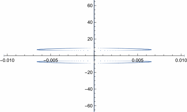
Figure 1 provides two examples of the numerically computed spectrum of (2.13). The periodic traveling waves are close together in $\triangle$ (see also Figure 4)—indeed, only the value of $\alpha$ differs slightly—and yet they exhibit a dramatic difference in the spectrum at $\pm i\infty$. In the left panel, for which (2.20) is elliptic (in a band), the spectrum lies apparently along the imaginary axis outside of some bounded set. In the right panel, on the other hand, the spectrum tends towards infinity along $\pm\sigma+i\mathbb{R}$, where $\sigma\approx 0.006726$, and $\sigma$ agrees well with $\frac{\log(|\mu|)}{T}$, where $\mu$ is numerically computed eigenvalue of the monodromy matrix of (2.20) such that $|\mu|>1$. Therefore the numerical result corroborates Theorem 2. There is a modulational instability to long wavelength perturbations near $0\in\mathbb{C}$ in both panels, although it is hard to distinguish at this scale. Also there is spectral instability to finite wavelength perturbations away from $0\in\mathbb{C}$ in the left panel.

In the left panel of Figure 2, for which (2.20) is in a gap—the second gap of the associated Lamé equation (see Section 2.4)—the numerically computed spectrum tends towards infinity along $\pm\sigma+i\mathbb{R}$, where $\sigma\approx 0.455$, far greater than the right panel of Figure 1, and $\sigma$ agrees well with $\frac{\log(|\mu|)}{T}$, where $\mu$ is the numerically computed eigenvalue of the monodromy matrix of (2.20) such that $|\mu|>1$. See also Figure 3 for modulational instability.

References

• [1] Jaime Angulo and Jose R. Quintero, Existence and orbital stability of cnoidal waves for a 1D Boussinesq equation, Int. J. Math. Math. Sci. (2007), Art. ID 52020, 36.
• [2] F. M. Arscott, Periodic differential equations. An introduction to Mathieu, Lamé, and allied functions, International Series of Monographs in Pure and Applied Mathematics, Vol. 66. A Pergamon Press Book, The Macmillan Co., New York, 1964.
• [3] T.B. Benjamin, J.L. Bona, and JJ. Mahony, Model equations for long waves in nonlinear dispersive systems, Philos. Trans. Roy. Soc. London Ser. A 272 (1972), 47–78.
• [4] D. J. Benney and J. C. Luke, On the interactions of permanent waves of finite amplitude, J. Math. and Phys. 43 (1964), 309–313.
• [5] J. L. Bona, M. Chen, and J.-C. Saut, Boussinesq equations and other systems for small-amplitude long waves in nonlinear dispersive media. I. Derivation and linear theory, J. Nonlinear Sci. 12 (2002), no. 4, 283–318.
• [6]   , Boussinesq equations and other systems for small-amplitude long waves in nonlinear dispersive media. II. The nonlinear theory, Nonlinearity 17 (2004), no. 3, 925–952.
• [7] J. Boussinesq, Théorie des ondes et des remous qui se propagent le long d’un canal rectangulaire horizontal, en communiquant au liquide contenu dans ce canal des vitesses sensiblement pareilles de la surface au fond, J. Math. Pures Appl. (2) 17 (1872), 55–108.
• [8] Jared C Bronski, Vera Mikyoung Hur, and Mathew A Johnson, Modulational instability in equations of KdV type, New approaches to nonlinear waves, Springer, 2016, pp. 83–133.
• [9] Jared C. Bronski, Vera Mikyoung Hur, and Samuel Lee Wester, Modulational instability for regularized long-wave models, In preparation (2021).
• [10] Jared C Bronski and Mathew A Johnson, The modulational instability for a generalized Korteweg–de Vries equation, Archive for rational mechanics and analysis 197 (2010), no. 2, 357–400.
• [11] Jared C Bronski, Mathew A Johnson, and Todd Kapitula, An index theorem for the stability of periodic travelling waves of Korteweg-de Vries type, Proceedings. Section A, Mathematics-The Royal Society of Edinburgh 141 (2011), no. 6, 1141.
• [12] Hongqiu Chen, Min Chen, and Nghiem V. Nguyen, Cnoidal wave solutions to Boussinesq systems, Nonlinearity 20 (2007), no. 6, 1443–1461.
• [13] Min Chen, Christopher W. Curtis, Bernard Deconinck, Crystal W. Lee, and Nghiem Nguyen, Spectral stability of stationary solutions of a Boussinesq system describing long waves in dispersive media, SIAM J. Appl. Dyn. Syst. 9 (2010), no. 3, 999–1018.
• [14] Carmen Chicone, Ordinary differential equations with applications, Texts in Applied Mathematics, vol. 34, Springer-Verlag, New York, 1999.
• [15] M. S. P. Eastham, The spectral theory of periodic differential equations, Texts in Mathematics (Edinburgh), Scottish Academic Press, Edinburgh; Hafner Press, New York, 1973.
• [16] Robert A. Gardner, Spectral analysis of long wavelength periodic waves and applications, Journal für die reine und angewandte Mathematik 1997 (1997), no. 491, 149–182.
• [17] Vera Mikyoung Hur and Ashish Kumar Pandey, Modulational instability in nonlinear nonlocal equations of regularized long wave type, Phys. D 325 (2016), 98–112.
• [18] Avinash Khare and Uday Sukhatme, New solvable and quasiexactly solvable periodic potentials, Journal of Mathematical Physics 40 (1999), no. 11, 5473–5494.
• [19] Ayşe Kiper, Fourier series coefficients for powers of the Jacobian elliptic functions, Mathematics of Computation 43 (1984), no. 167, 247–259.
• [20] D. J. Korteweg and G. de Vries, On the change of form of long waves advancing in a rectangular canal, and on a new type of long stationary waves, Philos. Mag. (5) 39 (1895), no. 240, 422–443.
• [21] Wilhelm Magnus and Stanley Winkler, Hill’s equation, Dover Publications, Inc., New York, 1979, Corrected reprint of the 1966 edition.
• [22] Georgios Pastras, The Weierstrass elliptic function and applications in classical and quantum mechanics, SpringerBriefs in Physics, Springer, Cham, [2020] ©2020, A primer for advanced undergraduates.
• [23] Robert L Pego and José Raúl Quintero, Two-dimensional solitary waves for a benney–luke equation, Physica D: Nonlinear Phenomena 132 (1999), no. 4, 476–496.
• [24] G. B. Whitham, Linear and nonlinear waves, Pure and Applied Mathematics (New York), John Wiley & Sons, Inc., New York, 1999, Reprint of the 1974 original, A Wiley-Interscience Publication.
• [25] E. T. Whittaker and G. N. Watson, A course of modern analysis, 1996, An introduction to the general theory of infinite processes and of analytic functions; with an account of the principal transcendental functions, Reprint of the fourth (1927) edition, pp. vi+608.
Appendix A The spectrum for the generalized KdV equation
Let θ∈[0,1]\theta\in[0,1] and we consider the spectral problem
λ​ϕ=ϕx​x​x−c​ϕx+θ​(u⁡(x)​ϕ)x,ϕ∈L2​(ℝ/2​π​ℤ),\lambda\phi=\phi_{xxx}-c\phi_{x}+\theta(u(x)\phi)_{x},\quad\phi\in L^{2}(\mathbb{R}/2\pi\mathbb{Z}), (A.1)
for some smooth and 2​π2\pi periodic function uu for some c≠−1,∈ℝc\neq-1,\in\mathbb{R}. We wish to show that the spectrum of (A.1) lies in the imaginary axis outside some bounded set. Let
ϕ⁡(x)=∑k∈ℤϕ^k​ei​k​xandu⁡(x)=∑k∈ℤu^k​ei​k​x,\phi(x)=\sum_{k\in\mathbb{Z}}\widehat{\phi}_{k}e^{ikx}\quad\text{and}\quad u(x)=\sum_{k\in\mathbb{Z}}\widehat{u}_{k}e^{ikx},
and we can reformulate (A.1) equivalently as
ϕ^k+i​θ​kλ+i​k3+i​c​k​∑n∈ℤu^n​ϕ^n−k=0,k∈ℤ.\widehat{\phi}_{k}+\frac{i\theta k}{\lambda+ik^{3}+ick}\sum_{n\in\mathbb{Z}}\widehat{u}_{n}\widehat{\phi}_{n-k}=0,\quad k\in\mathbb{Z}. (A.2)
Let
Sk={λ:|λ+i​k3+i​c​k|⩽k​∑n∈ℤ|u^n|}andS=⋃k∈ℤSk.S_{k}=\Big\{\lambda:|\lambda+ik^{3}+ick|\leqslant k\sum_{n\in\mathbb{Z}}|\widehat{u}_{n}|\Big\}\quad\text{and}\quad S=\bigcup_{k\in\mathbb{Z}}S_{k}.
We pause to remark that ∑n∈ℤ|u^n|<+∞\sum_{n\in\mathbb{Z}}|\widehat{u}_{n}|<+\infty because uu is smooth, whence |u^n|→0|\widehat{u}_{n}|\to 0 as |n|→∞|n|\to\infty more rapidly than polynomially. Observe that:
• •
The spectrum of (A.1) is contained in SS because if λ∉S\lambda\notin S then (A.2) is invertible of ϕ^k\widehat{\phi}_{k} for any k∈ℤk\in\mathbb{Z} for any θ∈[0,1]\theta\in[0,1];
SkS_{k} are disjoint when |k|≫1|k|\gg 1 because |ω⁡(k+1)−ω⁡(k)|→∞|\omega(k+1)-\omega(k)|\to\infty as |k|→∞|k|\to\infty, where ω⁡(k)=−k3−c​k\omega(k)=-k^{3}-ck is the dispersion relation of (A.1); For a regularized long-wave model, such as (1.3), on the other hand, |ω⁡(k+1)−ω⁡(k)||\omega(k+1)-\omega(k)| remains bounded for all k∈ℝk\in\mathbb{R};
λ\lambda is continuous in θ∈[0,1]\theta\in[0,1] and there is one in each SkS_{k} when θ=0\theta=0, whereby there is exactly one in each SkS_{k} when θ=1\theta=1.
To recapitulate, there are countably many SkS_{k} outside of a bounded set, each of which contains one eigenvalue of (A.1). Since (A.1) remains invariant under
λ↦λ∗andϕ↦ϕ∗\lambda\mapsto\lambda^{*}\quad\text{and}\quad\phi\mapsto\phi^{*}
where the asterisk denotes complex conjugation, and under
λ↦−λandx↦−x,\lambda\mapsto-\lambda\quad\text{and}\quad x\mapsto-x,
if there is one eigenvalue in each SkS_{k} then such an eigenvalue must lie in the imaginary axis. Therefore only finitely many eigenvalues can fall off the imaginary axis. The same will hold true for the quasi-periodic boundary condition.