OCT-GAN: Neural ODE-based Conditional Tabular GANsConference: Proceedings of the Web Conference 2021; April 19–23, 2021; Ljubljana, SloveniaProceedings of the Web Conference 2021 (WWW ’21), April 19–23, 2021, Ljubljana, SloveniaDOI: 10.1145/3442381.3449999ISBN: 978-1-4503-8312-7/21/04CCS: Computing methodologies Machine learningCCS: Computing methodologies Neural networks

GANs consist of two neural networks: a generator and a discriminator. They perform a two-play zero-sum game and its equilibrium state is theoretically well defined, where the generator achieves the optimal generation quality and the discriminator cannot distinguish between real and fake samples. WGAN and its variants are widely used among many GANs proposed so far (Arjovsky et al. 2017; Gulrajani et al. 2017; Adler and Lunz 2018). In particular, WGAN-GP is one of the most successful models and is defined as follows:

where $p_{\bm{z}}$ is a prior distribution; $p_{\bm{x}}$ is a distribution of data; G is a generator function; D is a discriminator (or Wasserstein critic) function; $\bar{\bm{x}}$ is a randomly weighted combination of $\texttt{G}(\bm{z})$ and $\bm{x}$. The discriminator provides feedback on the quality of the generation. In addition, we let $p_{g}$ be a distribution of fake data induced by the function $\texttt{G}(\bm{z})$ from $p_{\bm{z}}$, and $p_{\bar{\bm{x}}}$ be a distribution created after the random combination. We typically use $\mathcal{N}(\bm{0},\bm{1})$ for the prior $p_{\bm{z}}$. Many task-specific GAN models are designed on top of the WGAN-GP framework. We use $\mathcal{L}_{\texttt{D}},\mathcal{L}_{\texttt{G}}$ to denote the WGAN-GP’s loss functions to train the discriminator and the generator, respectively.

A popular variant of GANs are conditional GANs (Mirza and Osindero 2014; Isola et al. 2017). Under the regime of conditional GANs, the generator $\texttt{G}(\bm{z},\bm{c})$ is fed with a noisy vector $\bm{z}$ and a condition vector $\bm{c}$. In many cases, the condition vector is a one-hot vector denoting a class label to generate.

Tabular data synthesis, which generates a realistic synthetic table by modeling a joint probability distribution of columns in a table, encompasses many different methods depending on the types of data. For instance, Bayesian networks (Aviñó et al. 2018; Zhang et al. 2017) and decision trees (Reiter 2005) are used to generate discrete variables. A recursive modeling of tables using the Gaussian copula is used to generate continuous variables (Patki et al. 2016). A differentially private algorithm for decomposition is used to synthesize spatial data (Cormode et al. 2011; Zhang et al. 2016). However, some constraints that these models have such as the type of distributions and computational problems have hampered high-fidelity data synthesis.

In recent years, several data generation methods based on GANs have been introduced to synthesize tabular data, which mostly handle healthcare records. RGAN (Esteban et al. 2017) generates continuous time-series healthcare records while MedGAN (Choi et al. 2017), corrGAN (Patel et al. 2018) generate discrete records. EhrGAN (Che et al. 2017) generates plausible labeled records using semi-supervised learning to augment limited training data. PATE-GAN (Jordon et al. 2019) generates synthetic data without endangering the privacy of original data. TableGAN (Park et al. 2018) improved tabular data synthesis using convolutional neural networks to maximize the prediction accuracy on the label column.

Let $\bm{h}(t)$ be a function that outputs a hidden vector at time (or layer) $t$ in a neural network. In Neural ODEs (NODEs), a neural network $f$ with a set of parameters, denoted $\bm{\theta}_{f}$, approximates $\frac{d\bm{h}(t)}{dt}$, and $\bm{h}(t_{m})$ is calculated by $\bm{h}(t_{0})+\int_{t_{0}}^{t_{m}}f(\bm{h}(t),t;\bm{\theta}_{f})\,dt$, where $f(\bm{h}(t),t;\bm{\theta}_{f})=\frac{d\bm{h}(t)}{dt}$. In other words, the internal dynamics of the hidden vector evolution process is described by a system of ODEs parameterized by $\bm{\theta}_{f}$. One advantage of using NODEs is that we can interpret $t$ as continuous, which is discrete in usual neural networks. Therefore, more flexible constructions are possible in NODEs, which is one of the main reasons why we adopt an ODE layer in our discriminator.

To solve the integral problem, $\bm{h}(t_{0})+\int_{t_{0}}^{t_{m}}f(\bm{h}(t),t;\bm{\theta}_{f})\,dt$, in NODEs, we rely on an ODE solver which transforms an integral into a series of additions. The Dormand–Prince (DOPRI) method (Dormand and Prince 1980) is one of the most powerful integrators and is widely used in NODEs. It is a member of the Runge–Kutta family of ODE solvers. DOPRI dynamically controls its step size while solving an integral problem. It is now the default method in MATLAB, GNU Octave, etc.

Let $\phi_{t}:\mathbb{R}^{\dim(\bm{h}(t_{0}))}\rightarrow\mathbb{R}^{\dim(\bm{h}(t_{m}))}$ be a mapping from $t_{0}$ to $t_{m}$ created by an ODE after solving the integral problem. It is well-known that $\phi_{t}$ becomes a homeomorphic mapping: $\phi_{t}$ is continuous and bijective and $\phi_{t}^{-1}$ is also continuous for all $t\in[0,T]$, where $T$ is the last time point of the time domain (Dupont et al. 2019; Massaroli et al. 2020). From this characteristic, the following proposition can be derived:

While preserving the topology, NODEs can perform machine learning tasks and it was shown in (Yan et al. 2020) that it increases the robustness of representation learning to adversarial attacks.

Instead of the backpropagation method, the adjoint sensitivity method is used to train NODEs for its efficiency and theoretical correctness (Chen et al. 2018). After letting $\bm{a}_{\bm{h}}(t)=\frac{d\mathcal{L}}{d\bm{h}(t)}$ for a task-specific loss $\mathcal{L}$, it calculates the gradient of loss w.r.t model parameters with another reverse-mode integral as follows:

$\nabla_{\bm{h}(0)}\mathcal{L}$ can also be calcualte in a similar way and we can propagate the gradient backward to layers earlier than the ODE if any. It is worth of mentioning that the space complexity of the adjoint sensitivity method is $\mathcal{O}(1)$ whereas using the backpropagation to train NODEs has a space complexity proportional to the number of DOPRI steps. Their time complexities are similar or the adjoint sensitivity method is slightly more efficient than that of the backpropagation. Therefore, we can train NODEs efficiently.

We consider tabular data with two types of columns: discrete columns, denoted {$D_{1}$, $D_{2}$, …, $D_{N_{D}}$}, and continuous columns, denoted {$C_{1}$, $C_{2}$, …, $C_{N_{C}}$}. Discrete values are transformed to one-hot vectors as usual. However, continuous values are preprocessed with a mode-specific normalization technique (Xu et al. 2019). GANs generating tabular data frequently suffer from mode collapse and irregular data distribution. By specifying modes before training, the mode-specific normalization can alleviate the problems. The $i_{th}$ raw sample $r_{i}$ (a row or record in the tabular data) can be written as $d_{i,1}$ $\oplus$ $d_{i,2}$ $\oplus$ … $\oplus$ $d_{i,N_{D}}$ $\oplus$ $c_{i,1}$ $\oplus$ $c_{i,2}$ $\oplus$ … $\oplus$ $c_{i,N_{C}}$, where $d_{i,j}$ (resp. $c_{i,j}$) is a value in column $D_{j}$ (resp. column $C_{j}$). After the following three steps, the raw sample $r_{i}$ is preprocessed to $x_{i}$.

1. (1)

   Each discrete values {$d_{i,1}$, $d_{i,2}$, …, $d_{i,N_{D}}$} are transformed to one-hot vector {$\bm{d}_{i,1}$, $\bm{d}_{i,2}$, …, $\bm{d}_{i,N_{D}}$}.

2. (2)

   Using the variational Gaussian mixture (VGM) model, we fit each continuous column $C_{j}$ to a Gaussian mixture. The fitted Gaussian mixture is $\Pr_{j}(c_{i,j})=\sum_{k=1}^{n_{j}}w_{j,k}\mathcal{N}(c_{i,j};\mu_{j,k},\sigma_{j,k})$, where $n_{j}$ is the number of modes (i.e., the number of Gaussian distributions) in columns $C_{j}$. $w_{j,k},\mu_{j,k},\sigma_{j,k}$ are a fitted weight, mean and standard deviation of $k_{th}$ Gaussian distribution.

3. (3)

   With a probability of $\Pr_{j}(k)=\frac{w_{j,k}\mathcal{N}(c_{i,j};\mu_{j,k},\sigma_{j,k})}{\sum_{p=1}^{n_{j}}w_{j,p}\mathcal{N}(c_{i,j};\mu_{j,p},\sigma_{j,p})}$, we sample an appropriate mode $k$ for $c_{i,j}$. We then normalize $c_{i,j}$ from the mode $k$ with its fitted standard deviation, and save the normalized value $\alpha_{i,j}$ and the mode information $\beta_{i,j}$. For example, if there are 4 modes and we pick the third mode, i.e., $k=3$, then $\alpha_{i,j}$ is $\frac{c_{i,j}-\mu_{3}}{4\sigma_{3}}$ and $\beta_{i,j}$ is $[0,0,1,0]$.

4. (4)

   As a result, $r_{i}$ is transformed to $x_{i}$ which is denoted as follows:

   $$x_{i}=\alpha_{i,1}\oplus\beta_{i,1}\oplus\cdots\oplus\alpha_{i,N_{c}}\oplus\beta_{i,N_{c}}\oplus\bm{d}_{i,1}\oplus\cdots\oplus\bm{d}_{i,N_{D}}.$$

We note that in $x_{i}$, we can specify the detailed mode-based information of $r_{i}$. Our discriminator and generator work with $x_{i}$ instead of $r_{i}$ for its clarification on modes. However, $x_{i}$ can be readily changed to $r_{i}$, once generated, using the fitted parameters of the Gaussian mixture.

We design a NODE-based discriminator and consider the trajectory of $\bm{h}(t)$, where $t\in[0,t_{m}]$, when predicting whether an input sample $x$ is real or fake. To this end, we use the following ODE-based discriminator that outputs $\texttt{D}(x)$ given a (preprocessed or generated) sample $x$:

where $\oplus$ means the concatenation operator, $\mathtt{Leaky}$ is the leaky ReLU, $\mathtt{Drop}$ is the dropout, and $\mathtt{FC}$ is the fully connected layer. The ODE function $f(\bm{h}(t),t;\bm{\theta}_{f})$ is defined as follows:

where $\mathtt{BN}$ is the batch normalization and $\mathtt{ReLU}$ is the rectified linear unit.

We note that the trajectory of $\bm{h}(t)$ is continuous in NODEs. However, it is difficult to consider continuous trajectories in training GANs. To discretize the trajectory of $\bm{h}(t)$, therefore, $t_{1},t_{2},\cdots,t_{m}$ are trained and $m$ is a hyperparameter in our proposed method. We also note that Eqs. (3) to (6) share the same parameter $\bm{\theta}_{f}$, which means they constitute a single system of ODEs but for the purpose of discretization we separate them. After letting $\bm{a}_{t}(t)=\frac{d\mathcal{L}}{dt}$, we use the following gradient definition (derived from the adjoint sensitivity method) to train $t_{i}$ for all $i$:

For the same reason above, $\nabla_{t_{i}}\mathcal{L}=\frac{d\mathcal{L}}{dt_{i}}=\bm{a}_{\bm{h}}(t_{i})f(\bm{h}(t_{i}),t_{i};\bm{\theta}_{f})$ where $i<m$. But we do not want to save any intermediate adjoint states for space complexity purposes and calculate the gradient with a reverse-mode integral as follows:

We note that we need to save only one adjoint sate $\bm{a}_{\bm{h}}(t_{m})$ and calculate $\nabla_{t_{i}}\mathcal{L}$ with the two functions $f$ and $\bm{a}_{\bm{h}}(t)$.

We typically use the last hidden vector $\bm{h}(t_{m})$ for classification. In our case, however, we use the entire trajectory for classification. When using only the last hidden vector, all needed information for classification should be correctly captured in it. In our setting, however, even two similar last hidden vectors can be easily distinguished if their intermediate trajectories are different at least at a value of $t$. In addition, we train $t_{i}$, which further improves the efficacy of the proposed method by finding key time points to distinguish trajectories. We note that training $t_{i}$ is impossible in usual neural networks because their layer constructions are discrete. Fig. 3 illustrates such an example that only our NODE-based discriminator with learnable intermediate time points can correctly classify, and Fig. 4 also shows that our method can address the problem of the limited learning representation of NODEs.

The proposed OCT-GAN is a conditional GAN and its generator reads a noisy vector as well as a condition vector to generate a fake sample. Our definition of the condition vector is as follows:

where $\bm{c}_{i}$ is either a zero vector or a random one-hot vector of the $i_{th}$ discrete column. We randomly decide $s\in\{1,2,\cdots,N_{D}\}$ and only $\bm{c}_{s}$ is a random one-hot vector and for all other $i\neq s$, $\bm{c}_{i}$ is a zero vector, i.e., we specify a discrete value in the $s_{th}$ discrete column.

Given an initial input $\bm{p}(0)=\bm{z}\oplus\bm{c}$, we feed it into an ODE layer to transform into another latent vector. We denote this transformed vector by $\bm{z}^{\prime}$. For this transformation, we use an ODE layer independent from the ODE layer in the discriminator as follows:

We fix the integral time to $[0,1]$ because any ODE in $[0,w]$, $w>0$, with $g$ can be reduced into a unit-time integral with $g^{\prime}$ by letting $g^{\prime}=\frac{g(\bm{p}(t),t;\bm{\theta}_{g})}{w}$.

As noted earlier, an ODE is a homeomorphic mapping. We exploit the characteristic to design a semantically reliable mapping (or transformation). GANs typically use a noisy vector sampled from a Gaussian distribution, which is known as sub-optimal (Karras et al. 2019). Thus, the transformation is needed in our case.

The Grönwall–Bellman inequality states that given an ODE $\phi_{t}$ and its two initial states $\bm{p}_{1}(0)=\bm{x}$ and $\bm{p}_{2}(0)=\bm{x}+\bm{\delta}$, there exists a constant $\tau$ such that $\|\phi_{t}(\bm{x})-\phi_{t}(\bm{x}+\bm{\delta})\|\leq exp(\tau)\|\bm{\delta}\|$ (Pachpatte 1997). In other words, two similar input vectors with small $\bm{\delta}$ will be mapped to close to each other within a boundary of $exp(\tau)\|\bm{\delta}\|$.

In addition, we do not extract $\bm{z}^{\prime}$ from intermediate time points so the generator’s ODE learns a homeomorphic mapping. Thus, the topology of the initial input vector space is maintained. The initial input vector $\bm{p}(0)$ contains non-trivial information on what to generate, e.g., condition, so we would like to maintain the relationships among initial input vectors while transforming them onto another latent vector space suitable for generation. Fig. 5 shows an example of our two-stage approach where i) the ODE layer finds a balancing distribution between the initial input distribution and the real data distribution and ii) the following procedures generate realistic fake samples. In particular, our transformation makes the interpolation of synthetic samples smooth, i.e., given two similar initial inputs, two similar synthetic samples are generated by the generator (as proved in the Grönwall–Bellman inequality) — we show these smooth interpolations in our experiment section. The proposed generator equipped with learning the optimal transformation is as follows:

where $\mathtt{Tanh}$ is the hyperbolic tangent, and $\mathtt{Gumbel}$ is the Gumbel-softmax to generate one-hot vectors. The ODE function $g(\bm{p}(t),t;\bm{\theta}_{g})$ is defined as follows:

where $\mathtt{Norm}(\bm{p})=\frac{\bm{p}}{\|\bm{p}\|_{2}}$.

As stated earlier, we specify a discrete value in a discrete column as a condition. Thus, it is required that $\hat{\bm{d}}_{s}=\bm{c}_{s}$, and we use a cross-entropy loss to enforce the match, denoted $\mathcal{L}_{matching}=H(\bm{c}_{s},\hat{\bm{d}}_{s})$. Another possible design choice is to copy $\bm{c}_{s}$ to $\hat{\bm{d}}_{s}$. However, we do not copy for a principled training of the generator.

We train OCT-GAN using the loss in Eq. (1) in conjunction with $\mathcal{L}_{matching}$ and its training algorithm is in Alg. 1. To train OCT-GAN, we need a real table $\mathtt{T}_{\textrm{train}}$, and a maximum epoch number $max\_epoch$. After creating a mini-batch $b$ (line 1), we perform the adversarial training (lines 1, 1), followed by updating $t_{i}$ with the custom gradient calculated by the adjoint sensitivity method (line 1).

The space complexity to calculate $\nabla_{t_{i}}\mathcal{L}$ is $\mathcal{O}(1)$ (see Section 3.2). Calculating $\nabla_{t_{j}}\mathcal{L}$ subsumes the computation of $\nabla_{t_{i}}\mathcal{L}$, where $t_{0}\leq t_{j}<t_{i}\leq t_{m}$. While solving the reverse-mode integral from $t_{m}$ to $t_{0}$, thus, we can retrieve $\frac{d\mathcal{L}}{dt_{i}}$ for all $i$. Therefore, the space complexity to calculate all the gradients is $\mathcal{O}(m)$ at line 1, which is additional overhead incurred by our method.

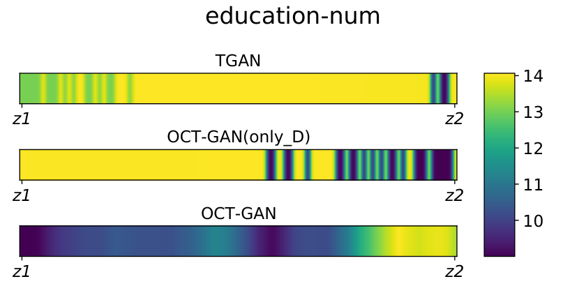
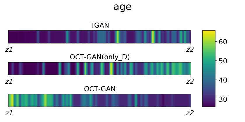
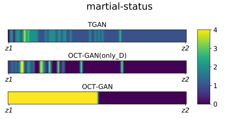
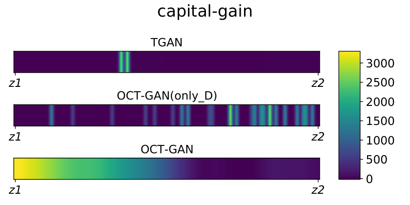
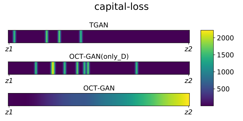
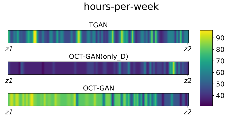
To further show the efficacy of the ODE-based transformation in the generator, we visualize several interpolation results in Adult. We select two noisy vectors $\bm{z}_{1},\bm{z}_{2}$ and interpolate many intermediate vectors by $e\bm{z}_{1}+(1-e)\bm{z}_{2}$, where $0<e<1$, to generate samples given a fixed random condition vector. In Fig. 6, we show those interpolation results in several columns of Adult. In our observation, TGAN and OCT-GAN(only_D) show similar interpolation patterns and OCT-GAN can interpolate in a smooth way.