Energy-preserving fully-discrete schemes for nonlinear stochastic wave equations with multiplicative noiseJournal: *

Jialin Hong Email: hjl@lsec.cc.ac.cn Address: Institute of Computational Mathematics and Scientific/Engineering Computing, Academy of Mathematics and Systems Science, Chinese Academy of Sciences, Beijing 100190, China Address: School of Mathematical Sciences, University of Chinese Academy of Sciences, Beijing 100049, China Baohui Hou Email: houbaohui@lsec.cc.ac.cn Corresponding author: Corresponding author Address: Institute of Computational Mathematics and Scientific/Engineering Computing, Academy of Mathematics and Systems Science, Chinese Academy of Sciences, Beijing 100190, China Liying Sun Email: liyingsun@lsec.cc.ac.cn Address: Institute of Computational Mathematics and Scientific/Engineering Computing, Academy of Mathematics and Systems Science, Chinese Academy of Sciences, Beijing 100190, China

Abstract

In this paper, we focus on constructing numerical schemes preserving the averaged energy evolution law for nonlinear stochastic wave equations driven by multiplicative noise. We first apply the compact finite difference method and the interior penalty discontinuous Galerkin finite element method to discretize space variable and present two semi-discrete schemes, respectively. Then we make use of the discrete gradient method and the Padé approximation to propose efficient fully-discrete schemes. These semi-discrete and fully-discrete schemes are proved to preserve the discrete averaged energy evolution law. In particular, we also prove that the proposed fully-discrete schemes exactly inherit the averaged energy evolution law almost surely if the considered model is driven by additive noise. Numerical experiments are given to confirm theoretical findings.

Keywords:

Compact finite difference method , Interior penalty discontinuous Galerkin finite element method , Padé approximation , Averaged energy evolution law , Stochastic wave equation , Multiplicative noise

1 Introduction

The nonlinear stochastic wave equation plays an important role in a wide range of applications in the field of engineering, science, etc., and is commonly used to describe a variety of physical processes, such as the motion of a strand of DNA in a liquid, the motion of shock waves on the surface of the sun, the dynamics of the primary current density vector field within the grey matter of the human brain and the sound propagation in the sea and so on (see e.g., [3, 7, 8, 11] and references therein). In this paper, we consider the following nonlinear stochastic wave equation driven by multiplicative noise

\left\{\begin{aligned} &du=vdt,&&(x,t)\in(a,b)\times(0,T],\\ &dv=\Delta udt-f(u)dt+g(u)dW(t),&&(x,t)\in(a,b)\times(0,T],\\ &u(x,0)=u_{0}(x),v(x,0)=v_{0}(x),&&x\in[a,b],\end{aligned}\right.

(1.1)

where $u_{0}$ and $v_{0}$ are real-valued deterministic functions, and $\Delta$ is the Laplace operator with Dirichlet or periodic boundary condition. Here, $\{W(t)\}_{t\geq 0}$ is an $\mathscr{H}$ -valued $Q$ -Wiener process with respect to a normal filtration $\{\mathcal{F}_{t}\}_{t\geq 0}$ on a filtered probability space $(\Omega,\mathcal{F},\{\mathcal{F}_{t}\}_{t\geq 0},\mathbb{P})$ and has the form of

W(t)=\sum_{k=1}^{\infty}\sqrt{q_{k}}e_{k}\beta_{k}(t),

where $\mathscr{H}=L^{2}([a,b];\mathbb{R})$ , $\{(q_{k},e_{k})\}_{k=1}^{\infty}$ are eigenpairs of symmetric, positive definite and finite trace operator $Q$ with orthonormal eigenvectors and $\{\beta_{k}(t)\}_{k=1}^{\infty}$ is a sequence of real-valued mutually independent standard Brownian motions. Assume that $f:\mathscr{H}\rightarrow\mathscr{H}$ and $g(u):\mathscr{H}\rightarrow\mathscr{L}_{2}^{0}$ satisfy the global Lipschitz condition, where $\mathscr{L}_{2}^{0}=\mathscr{L}_{2}(\mathscr{H},\mathscr{H}_{0})$ denotes the separable Hilbert space of Hilbert-Schmidt operators from $\mathscr{H}$ to $\mathscr{H}_{0}$ with $\mathscr{H}_{0}=Q^{\frac{1}{2}}(\mathscr{H})$ . For the well-posedness of (1.1), we refer readers to [1, 24]. It has been shown that the averaged energy of the nonlinear stochastic wave equation (1.1) satisfies the following identity

\mathbb{E}[H(u(t),v(t))]=\mathbb{E}[H(u(0),v(0))]+\frac{1}{2}\mathbb{E}\left[\int_{0}^{t}Tr\left((g(u)Q^{\frac{1}{2}})(g(u)Q^{\frac{1}{2}})^{*}\right)ds\right],

(1.2)

where

H(u,v)=\frac{1}{2}\int_{a}^{b}\left(v^{2}+\left(\frac{\partial u}{\partial x}\right)^{2}\right)dx+\int_{a}^{b}\widetilde{f}\left(u\right)dx,

(1.3)

and $f=\frac{\partial\widetilde{f}}{\partial u}$ . In particular, when $g(u)=\lambda$ with $\lambda$ being a positive constant, (1.1) becomes a nonlinear stochastic wave equation driven by additive noise. It is shown in (1.2) that the averaged energy increases linearly with respect to the evolution of time with a growth rate $\frac{\lambda^{2}}{2}Tr(Q)$ . (1.2) is also related to the energy equation, which is a tool that can be used to analyze the existence or nonexistence of solutions to nonlinear stochastic wave equations (see [1]).

It is well-known that numerical simulations are often used to understand the behavior of the solutions for stochastic partial differential equations. Especially, numerical schemes preserving energy evolution law often yield physically correct results and numerical stability in computation. Much effort has been devoted to the numerical method of stochastic wave equations (see e.g., [1, 3, 6, 8, 9, 10, 16, 21, 26] and references therein). For instance, [8] proves that the fully-discrete scheme based on the finite element method and the stochastic trigonometric scheme preserves the linear growth of the averaged energy for the linear stochastic wave equation with additive noise. With regard to the nonlinear stochastic wave equation with additive noise, [3] shows that the discontinuous Galerkin finite element method satisfies the trace formula. [10] proposes a full discretization by adopting the spectral Galerkin method and the averaged vector field method preserving the averaged energy evolution law of the stochastic cubic wave equation with additive noise. In [1], the authors utilize the standard linear finite element approximation and a stochastic trigonometric method to propose a fully-discrete scheme for the nonlinear stochastic wave equation driven by multiplicative noise, and prove that this numerical scheme satisfies an almost trace formula for the case of the additive noise. To the best of knowledge, there has not been a fully-discrete scheme which can exactly preserve the averaged energy evolution law of nonlinear stochastic wave equations driven by multiplicative noise.

In this paper, we aim to propose fully-discrete schemes preserving averaged energy evolution law for nonlinear stochastic wave equations driven by multiplicative noise (1.1). Motivated by the fact that the compact finite difference method enjoys the flexibility to handle the boundary conditions and could achieve high-order accuracy with smaller stencils and the fact that the interior penalty discontinuous Galerkin finite element method is particularly suitable to deal with complex computational domains and is easy to design high-order approximations, we apply these two numerical schemes to discretizing (1.1) and obtain two semi-discrete schemes in space. We prove that the resulting finite dimensional stochastic differential equations preserve the discrete version of the averaged energy evolution law of the original system. Besides numerical schemes in space, the energy-preserving fully-discrete scheme also depends on the numerical schemes in time, which confronts the difficulty brought by the treatment of the time approximation on both drift and diffusion coefficients. For example, if we make use of the discrete gradient method to the nonlinear drift term and the explicit Euler method to the diffusion term for semi-discrete scheme, which is given by means of the compact finite difference in spatial direction, of the nonlinear stochastic wave equation (1.1), the averaged energy of the obtained fully-discrete scheme is more $\frac{1}{2}h\Delta t\mathbb{E}\left[(\frac{1}{2}\mathbf{A^{-1}D}(\mathbf{U}^{n+1}+\mathbf{U}^{n})-\overline{\nabla}_{U}\mathbf{F}(\mathbf{U}^{n+1},\mathbf{U}^{n}))G(\mathbf{U}^{n})\mathbf{E}\boldsymbol{\Lambda}\Delta\boldsymbol{\beta}_{n}\right]$ than that of the original stochastic system (the concrete meanings of symbols are given below). To overcome this difficulty, we discretize the solution given by the constant variation method of aforementioned two semi-discrete schemes based on the discrete gradient method and the Padé approximation. We prove that the proposed fully-discrete schemes admit the discrete averaged energy evolution law, which is consistent with the averaged energy evolution law of (1.1). We would like to mention that the proposed fully-discrete schemes are flexible due to the flexibility of the Padé approximation. Finally, numerical experiments confirm the theoretical analysis results.

The paper is organized as follows. In Section 2, we employ the compact finite difference method and the interior penalty discontinuous Galerkin finite element method to obtain two semi-discrete schemes, and prove that both of them possess discrete averaged energy evolution laws. Then the discrete gradient method and the Padé approximation are ulitized to construct fully-discrete schemes, and the conservation of discrete averaged energy evolution laws is proved in Section 3. Numerical experiments are carried out in Section 4. Finally, the conclusion is given in Section 5.

2 Energy-preserving semi-discrete schemes in space

In this section, we investigate the compact finite difference method and the interior penalty discontinuous Galerkin finite element method for the nonlinear stochastic wave equation (1.1), respectively. Then we prove that these semi-discrete schemes preserve the averaged energy evolution laws for (1.1) below. Denote the uniform partition of $[a,b]$ by $\{x_{i}\}_{0\leq i\leq M}$ with $x_{i}=a+ih$ , where $M$ is a positive integer, and $h:=(b-a)/M$ denotes the spatial step size.

2.1 Semi-discrete scheme via the compact finite difference method

The compact finite difference method, as the high accuracy discrete method utilizing smaller stencils and treating boundary conditions easily, has been extensively studied in [5, 12, 19]. We first apply the compact finite difference method to discretizing the nonlinear stochastic wave equation (1.1) with Dirichlet boundary condition. Now we introduce the discrete grid $\Omega_{h}=\{x_{i}|~1\leq i\leq M-1\}$ , and difference operators $\delta_{x}^{2}$ and $\mathcal{A}$ defined as

\quad\delta_{x}^{2}u_{i}=\frac{u_{i-1}-2u_{i}+u_{i+1}}{h^{2}},\qquad\mathcal{A}u_{i}=\left(1+\frac{h^{2}}{12}\delta_{x}^{2}\right)u_{i}

for any grid function $u=\{u_{i}|~x_{i}\in\Omega_{h},u_{0}=u_{M}=0\}$ . From [14, 19], it can be verified that the compact finite difference operator $\mathcal{A}^{-1}\delta_{x}^{2}$ satisfies

\mathcal{A}^{-1}\delta_{x}^{2}u_{i}=\frac{\partial^{2}u}{\partial x^{2}}(x_{i})+O(h^{4}),\quad 1\leq i\leq M-1.

Based on the above operator, the compact finite difference method for (1.1) with Dirichlet boundary condition reads

\left\{\begin{aligned} dU_{i}&=V_{i}dt,\\ dV_{i}&=\mathcal{A}^{-1}\delta_{x}^{2}U_{i}dt-f(U_{i})dt+g(U_{i})\sum_{k=1}^{P}\sqrt{q_{k}}e_{k}(x_{i})d\beta_{k}(t),\end{aligned}\right.

(2.1)

where $U_{i},V_{i}$ are the approximations of $u_{i}=u(x_{i},t),v_{i}=v(x_{i},t)$ , respectively, for $1\leq i\leq M-1$ . Denote

		$\displaystyle\mathbf{U}=\left(U_{1},U_{2},\dots,U_{M-1}\right)^{\top},\quad$		$\displaystyle\mathbf{V}=\left(V_{1},V_{2},\dots,V_{M-1}\right)^{\top},$
		$\displaystyle\boldsymbol{\Lambda}={\rm{diag}}\{\sqrt{q_{1}},\sqrt{q_{2}},\dots,\sqrt{q_{P}}\},\quad$		$\displaystyle\boldsymbol{\beta}=\left(\beta_{1},\beta_{2},\dots,\beta_{P}\right)^{\top},$
		$\displaystyle F(\mathbf{U})=\left(f(U_{1}),f(U_{2}),\dots,f(U_{M-1})\right)^{\top},\quad$		$\displaystyle G(\mathbf{U})={\rm{diag}}\{g(U_{1}),g(U_{2}),\dots,g(U_{M-1})\}$

and

\mathbf{E}={\left[\begin{array}[]{cccc}e_{1}(x_{1})&e_{2}(x_{1})&\cdots&e_{P}(x_{1})\\ e_{1}(x_{2})&e_{2}(x_{2})&\cdots&e_{P}(x_{2})\\ \vdots&\vdots&&\vdots\\ e_{1}(x_{M-1})&e_{2}(x_{M-1})&\cdots&e_{P}(x_{M-1})\\ \end{array}\right]_{(M-1)\times P}}.

Define matrices $\mathbf{D}$ and $\mathbf{A}$ of order $(M-1)\times(M-1)$ as

\mathbf{D}=\frac{1}{h^{2}}{\left[\begin{array}[]{cccccccc}-2&1&0&0&\cdots&0&0&0\\[3.61371pt] 1&-2&1&0&\cdots&0&0&0\\ \vdots&\vdots&\vdots&\vdots&&\vdots&\vdots&\vdots\\ 0&0&0&0&\cdots&1&-2&1\\[3.61371pt] 0&0&0&0&\cdots&0&1&-2\end{array}\right]},\quad\mathbf{A}={\left[\begin{array}[]{cccccccc}\frac{10}{12}&\frac{1}{12}&0&0&\cdots&0&0&0\\[3.61371pt] \frac{1}{12}&\frac{10}{12}&\frac{1}{12}&0&\cdots&0&0&0\\ \vdots&\vdots&\vdots&\vdots&&\vdots&\vdots&\vdots\\ 0&0&0&0&\cdots&\frac{1}{12}&\frac{10}{12}&\frac{1}{12}\\[3.61371pt] 0&0&0&0&\cdots&0&\frac{1}{12}&\frac{10}{12}\end{array}\right]},

(2.2)

which are arising from the operator $\delta_{x}^{2}$ and $\mathcal{A}$ , respectively. In addition, let $\mathbf{A^{-1}D}$ be the matrix associated to operator $\mathcal{A}^{-1}\delta_{x}^{2}$ . Then we can rewrite (2.1) into

\left\{\begin{aligned} d\mathbf{U}&=\mathbf{V}dt,\\ d\mathbf{V}&=\mathbf{A^{-1}D}\mathbf{U}dt-F(\mathbf{U})dt+G(\mathbf{U})\mathbf{E}\boldsymbol{\Lambda}d\boldsymbol{\beta}.\\ \end{aligned}\right.

(2.3)

The semi-discrete scheme (2.3) preserves the discrete version of stochastic energy evolution law, which is stated in the following theorem.

Theorem 2.1.

The averaged energy for semi-discrete scheme (2.3) has the following evolutionary relationship

\mathbb{E}\left[\bar{H}(\mathbf{U}(t),\mathbf{V}(t))\right]=\mathbb{E}\left[\bar{H}(\mathbf{U}(0),\mathbf{V}(0))\right]+\frac{h}{2}\mathbb{E}\left[\int_{0}^{t}Tr(G^{2}(\mathbf{U})\mathbf{E}\boldsymbol{\Lambda}^{2}\mathbf{E}^{\top})ds\right],

(2.4)

where

\bar{H}(\mathbf{U}(t),\mathbf{V}(t))=\frac{1}{2}\sum_{i=1}^{M-1}hV_{i}^{2}(t)-\frac{1}{2}\sum_{i=1}^{M-1}hU_{i}(t)\mathcal{A}^{-1}\delta_{x}^{2}U_{i}(t)+\sum_{i=1}^{M-1}h\widetilde{f}(U_{i}(t))

is the discrete energy with respect to (1.3).

Proof. Based on Itô’s formula for $\frac{1}{2}\sum_{i=1}^{M-1}hV_{i}^{2}$ , we obtain

$\displaystyle\frac{1}{2}\sum_{i=1}^{M-1}hV_{i}^{2}(t)$	$\displaystyle=\frac{1}{2}\sum_{i=1}^{M-1}hV_{i}^{2}(0)+\int_{0}^{t}\sum_{i=1}^{M-1}hV_{i}(s)g(U_{i}(s))\sum_{k=1}^{P}\sqrt{q_{k}}e_{k}(x_{i})d\beta_{k}(s)$	(2.5)
	$\displaystyle+\int_{0}^{t}\sum_{i=1}^{M-1}hV_{i}(s)(\mathcal{A}^{-1}\delta_{x}^{2}U_{i}(s))ds-\int_{0}^{t}\sum_{i=1}^{M-1}hV_{i}(s)f(U_{i}(s))ds$
	$\displaystyle+\frac{1}{2}\int_{0}^{t}h\sum_{i=1}^{M-1}\sum_{k=1}^{P}g^{2}(U_{i}(s))q_{k}e_{k}^{2}(x_{i})ds.$

Direct calculations yield

	$\displaystyle\int_{0}^{t}\sum_{i=1}^{M-1}hV_{i}(s)(\mathcal{A}^{-1}\delta_{x}^{2}U_{i}(s))ds$	$\displaystyle=\int_{0}^{t}\sum_{i=1}^{M-1}\frac{h}{2}d\left(U_{i}(s)\mathcal{A}^{-1}\delta_{x}^{2}U_{i}(s)\right)$		(2.6)
		$\displaystyle=\sum_{i=1}^{M-1}\frac{h}{2}\left(U_{i}(t)\mathcal{A}^{-1}\delta_{x}^{2}U_{i}(t)-U_{i}(0)\mathcal{A}^{-1}\delta_{x}^{2}U_{i}(0)\right),$		(2.6)

-\int_{0}^{t}\sum_{i=1}^{M-1}hV_{i}(s)f(U_{i}(s))ds=-\int_{0}^{t}\sum_{i=1}^{M-1}hd\widetilde{f}(U_{i}(s))=-\sum_{i=1}^{M-1}h\left(\widetilde{f}(U_{i}(t))-\widetilde{f}(U_{i}(0))\right).

(2.7)

Combining the definition of $\bar{H}(\mathbf{U}(t),\mathbf{V}(t))$ as follows

\bar{H}(\mathbf{U}(t),\mathbf{V}(t))=\frac{1}{2}\sum_{i=1}^{M-1}hV_{i}^{2}(t)-\frac{1}{2}\sum_{i=1}^{M-1}hU_{i}(t)\mathcal{A}^{-1}\delta_{x}^{2}U_{i}(t)+\sum_{i=1}^{M-1}h\widetilde{f}(U_{i}(t))

(2.8)

and (2.6), (2.7), then (2.5) can be rewritten as

	$\displaystyle\bar{H}(\mathbf{U}(t),\mathbf{V}(t))$	$\displaystyle=\bar{H}(\mathbf{U}(0),\mathbf{V}(0))+\int_{0}^{t}\sum_{i=1}^{M-1}hV_{i}(s)g(U_{i}(s))\sum_{k=1}^{P}\sqrt{q_{k}}e_{k}(x_{i})d\beta_{k}(s)$		(2.9)
		$\displaystyle+\frac{h}{2}\int_{0}^{t}\sum_{i=1}^{M-1}\sum_{k=1}^{P}g^{2}(U_{i}(s))q_{k}e_{k}^{2}(x_{i})ds.$		(2.9)

Taking expectation, we derive

\mathbb{E}\left[\bar{H}(\mathbf{U}(t),\mathbf{V}(t))\right]=\mathbb{E}\left[\bar{H}(\mathbf{U}(0),\mathbf{V}(0))\right]+\frac{h}{2}\mathbb{E}\left[\int_{0}^{t}Tr(G^{2}(\mathbf{U})\mathbf{E}\boldsymbol{\Lambda}^{2}\mathbf{E}^{\top})ds\right],

which completes the proof. $\square$

Remark 2.2.

If we consider the nonlinear stochastic wave equation (1.1) with periodic boundary condition, the corresponding matrices associated to operator $\delta_{x}^{2}$ and $\mathcal{A}$ are

\mathbf{D}_{p}=\frac{1}{h^{2}}{\left[\begin{array}[]{cccccccc}-2&1&0&0&\cdots&0&0&1\\[3.61371pt] 1&-2&1&0&\cdots&0&0&0\\ \vdots&\vdots&\vdots&\vdots&&\vdots&\vdots&\vdots\\ 0&0&0&0&\cdots&1&-2&1\\[3.61371pt] 1&0&0&0&\cdots&0&1&-2\end{array}\right]},\quad\mathbf{A}_{p}={\left[\begin{array}[]{cccccccc}\frac{10}{12}&\frac{1}{12}&0&0&\cdots&0&0&\frac{1}{12}\\[3.61371pt] \frac{1}{12}&\frac{10}{12}&\frac{1}{12}&0&\cdots&0&0&0\\ \vdots&\vdots&\vdots&\vdots&&\vdots&\vdots&\vdots\\ 0&0&0&0&\cdots&\frac{1}{12}&\frac{10}{12}&\frac{1}{12}\\[3.61371pt] \frac{1}{12}&0&0&0&\cdots&0&\frac{1}{12}&\frac{10}{12}\end{array}\right]},

where $\mathbf{D}_{p}$ and $\mathbf{A}_{p}$ are matrices of order $M\times M$ . Also, the corresponding semi-discrete scheme discretized by the compact finite difference method is

\left\{\begin{aligned} d\mathbf{U}&=\mathbf{V}dt,\\ d\mathbf{V}&=\mathbf{A}_{p}^{-1}\mathbf{D}_{p}\mathbf{U}dt-F(\mathbf{U})dt+G(\mathbf{U})\mathbf{E}_{p}\boldsymbol{\Lambda}d\boldsymbol{\beta},\\ \end{aligned}\right.

(2.10)

where $\mathbf{U}=\left(U_{1},U_{2},\dots,U_{M}\right)^{\top}$ , $\mathbf{V}=\left(V_{1},V_{2},\dots,V_{M}\right)^{\top}$ , $F(\mathbf{U})=\left(f(U_{1}),f(U_{2}),\dots,f(U_{M})\right)^{\top}$ , $G(\mathbf{U})={\rm{diag}}(g(U_{1}),g(U_{2}),\dots,g(U_{M}))$ and $\mathbf{E}_{p}=(e_{i}(x_{k}))$ for $i\in\{1,2,\dots,P\},k\in\{1,2,\dots,M\}$ . Similarly, the semi-discrete scheme (2.10) of the nonlinear stochastic wave equation with periodic boundary condition possesses the averaged energy evolution law, i.e.,

\mathbb{E}\left[\bar{\bar{H}}(\mathbf{U}(t),\mathbf{V}(t))\right]=\mathbb{E}\left[\bar{\bar{H}}(\mathbf{U}(0),\mathbf{V}(0))\right]+\frac{h}{2}\mathbb{E}\left[\int_{0}^{t}Tr(G^{2}(\mathbf{U})\mathbf{E}_{p}\boldsymbol{\Lambda}^{2}\mathbf{E}_{p}^{\top})ds\right],

where

\bar{\bar{H}}(\mathbf{U}(t),\mathbf{V}(t))=\frac{1}{2}\sum_{i=1}^{M}hV_{i}^{2}(t)-\frac{1}{2}h\mathbf{U}(t)^{\top}\mathbf{A}_{p}^{-1}\mathbf{D}_{p}\mathbf{U}+\sum_{i=1}^{M}h\widetilde{f}(U_{i}(t)).

2.2 Semi-discrete scheme via the interior penalty discontinuous Galerkin finite element method

The discontinuous Galerkin finite element method is flexible to deal with the complex computational domain and is easy to construct locally high-order approximations, which has been extensively studied in [2, 3, 17]. In this subsection, we discretize (1.1) with Dirichlet boundary condition by using the interior penalty discontinuous Galerkin finite element method in space. Here, we use the same uniform mesh division of $[a,b]$ as in Subsection 2.1, denote $I_{i}=(x_{i},x_{i+1})$ , and define the discontinuous polynomial space as follows

V_{h}=\{u\in L^{2}([a,b]):u|_{I_{i}}\in\mathcal{P}^{k},~u(a)=u(b)=0~~\forall~i=0,1,\dots,M-1\},

where $\mathcal{P}^{k}$ denotes the polynomials of degree less or equal to $k\geq 1$ . Moreover, let

u(x_{i}^{+})=\lim_{\begin{subarray}{c}\epsilon\rightarrow 0\\ \epsilon>0\end{subarray}}u(x_{i}+\epsilon),\qquad u(x_{i}^{-})=\lim_{\begin{subarray}{c}\epsilon\rightarrow 0\\ \epsilon>0\end{subarray}}u(x_{i}-\epsilon).

Then we define the jump and average of $u$ at the endpoints of $I_{i}$ as follows

\llbracket{u(x_{i})}\rrbracket=u(x_{i}^{-})-u(x_{i}^{+}),\quad\boldsymbol{\{}u(x_{i})\boldsymbol{\}}=\frac{1}{2}\left(u(x_{i}^{-})+u(x_{i}^{+})\right)\quad\forall~i=1,2,\dots,M-1.

By convention, we also extend the definition of jump and average at the endpoints of the unit interval

	$\displaystyle$	$\displaystyle\llbracket{u(x_{0})}\rrbracket=-u(x_{0}^{+}),\quad~~\boldsymbol{\{}u(x_{0})\boldsymbol{\}}=u(x_{0}^{+}),$		(2.11)
		$\displaystyle\llbracket{u(x_{M})}\rrbracket=u(x_{M}^{-}),\quad~~\boldsymbol{\{}u(x_{M})\boldsymbol{\}}=u(x_{M}^{-}).$		(2.11)

Multiplying (1.1) by $\xi(x)$ and integrating by parts on each interval $I_{i}$ , with $\xi(x)$ being a function in $V_{h}$ for $i\in\{1,2,\dots,M-1\}$ , we get

\int_{x_{i}}^{x_{i+1}}\Delta u(x)\xi(x)dx=-\int_{x_{i}}^{x_{i+1}}\nabla u(x)\nabla\xi(x)dx+\nabla u(x_{i+1}^{-})\xi(x_{i+1}^{-})-\nabla u(x_{i}^{+})\xi(x_{i}^{+}).

Summing above equation from $i=0$ to $M-1$ , and using (2.11), we have

\sum_{i=0}^{M-1}\int_{x_{i}}^{x_{i+1}}\Delta u(x)\xi(x)dx=-\sum_{i=0}^{M-1}\int_{x_{i}}^{x_{i+1}}\nabla u(x)\nabla\xi(x)dx+\sum_{i=0}^{M}\llbracket{\nabla u(x_{i})\xi(x_{i})}\rrbracket.

(2.12)

It can be verified that

\llbracket{\nabla u(x_{i})\xi(x_{i})}\rrbracket=\boldsymbol{\{}\nabla u(x_{i})\boldsymbol{\}}\llbracket{\xi(x_{i})}\rrbracket+\boldsymbol{\{}\xi(x_{i})\boldsymbol{\}}\llbracket{\nabla u(x_{i})}\rrbracket,\quad 1\leq i\leq M-1.

Due to the fact that the exact solution satisfies $\boldsymbol{\{}\xi(x_{i})\boldsymbol{\}}\llbracket{\nabla u(x_{i})}\rrbracket=0$ for $0\leq i\leq M$ , (2.12) becomes

\sum_{i=0}^{M-1}\int_{x_{i}}^{x_{i+1}}\Delta u(x)\xi(x)dx=-\sum_{i=0}^{M-1}\int_{x_{i}}^{x_{i+1}}\nabla u(x)\nabla\xi(x)dx+\sum_{i=0}^{M}\boldsymbol{\{}\nabla u(x_{i})\boldsymbol{\}}\llbracket{\xi(x_{i})}\rrbracket.

Let $B_{h}$ be the symmetric interior penalty discrete bilinear form

	$\displaystyle B_{h}(u,\xi)$	$\displaystyle=-\sum_{i=0}^{M-1}\int_{x_{i}}^{x_{i+1}}\nabla u(x)\nabla\xi(x)dx+\sum_{i=0}^{M}\boldsymbol{\{}\nabla u(x_{i})\boldsymbol{\}}\llbracket{\xi(x_{i})}\rrbracket$		(2.13)
		$\displaystyle+\sum_{i=0}^{M}\boldsymbol{\{}\nabla\xi(x_{i})\boldsymbol{\}}\llbracket{u(x_{i})}\rrbracket-\sum_{i=0}^{M}\frac{\sigma}{h}\llbracket{u(x_{i})}\rrbracket\llbracket{\xi(x_{i})}\rrbracket,$		(2.13)

where the positive constant $\sigma$ is the interior penalty stabilization parameter. The third term in the right hand of (2.13) makes the bilinear form symmetric and the last term ensures coercivity of the bilinear with sufficiently large $\sigma$ . The bilinear form $B_{h}(\cdot,\cdot)$ defines a discrete linear operator $\Delta_{h}:V_{h}\rightarrow V_{h}$ as

\langle\Delta_{h}U,\xi\rangle=B_{h}(U,\xi)\quad\forall~\xi\in V_{h},

where $\langle\cdot,\cdot\rangle$ is the inner product in $L^{2}([a,b])$ .

As a consequence, the discrete formulation is given by: find $U,V\in V_{h}$ such that

\left\{\begin{aligned} dU&=Vdt,\\ dV&=\Delta_{h}Udt-P_{h}f(U)dt+P_{h}g(U)dW(t),\\ \end{aligned}\right.

(2.14)

where $P_{h}:L^{2}([a,b])\rightarrow V_{h}$ is the projection. Analogous to (2.3), the semi-discrete scheme (2.14) preserves the following discrete version of energy evolution law.

Theorem 2.3.

The averaged energy for semi-discrete scheme (2.14) has the following evolutionary relationship

\mathbb{E}\left[\widehat{H}(U(t),V(t))\right]=\mathbb{E}\left[\widehat{H}(U(0),V(0))\right]+\frac{1}{2}\mathbb{E}\left[\int_{0}^{t}Tr\left(P_{h}g(U)Q(P_{h}g(U))^{*}\right)ds\right],

(2.15)

where

\widehat{H}(U(t),V(t))=\frac{1}{2}\langle V(t),V(t)\rangle-\frac{1}{2}\langle\Delta_{h}U(t),U(t)\rangle+\int_{a}^{b}P_{h}\widetilde{f}(U(t))dx

is the discrete energy with respect to (1.3).

Proof. By the Itô’s formula for $\frac{1}{2}\int_{a}^{b}V(t)^{\top}V(t)dx=\frac{1}{2}\langle V(t),V(t)\rangle$ , we deduce

	$\displaystyle\frac{1}{2}\langle V(t),V(t)\rangle$	$\displaystyle=\frac{1}{2}\langle V(0),V(0)\rangle+\int_{0}^{t}\langle V(s),P_{h}g(U(s))dW(s)\rangle+\int_{0}^{t}\langle V(s),\Delta_{h}U(s)-P_{h}f(U(s))\rangle ds$		(2.16)
		$\displaystyle+\frac{1}{2}\int_{0}^{t}Tr\big[(P_{h}g(U)Q^{\frac{1}{2}})(P_{h}g(U)Q^{\frac{1}{2}})^{*}\big]ds.$		(2.16)

Using the first equation of (2.14), we get

$\displaystyle$	$\displaystyle\int_{0}^{t}\langle V(t),\Delta_{h}U(s)-P_{h}f(U(s))\rangle ds$	(2.17)
	$\displaystyle=\int_{0}^{t}\left\langle\frac{dU(s)}{ds},\Delta_{h}U(s)\right\rangle ds-\int_{a}^{b}\int_{0}^{t}\frac{dU(s)}{ds}P_{h}f(U(s))dsdx$
	$\displaystyle=\frac{1}{2}\langle\Delta_{h}U(s),U(s)\rangle\Big\|_{0}^{t}-\int_{a}^{b}P_{h}\widetilde{f}(U(s))\Big\|_{0}^{t}dx$
	$\displaystyle=\frac{1}{2}\langle\Delta_{h}U(t),U(t)\rangle-\frac{1}{2}\langle\Delta_{h}U(0),U(0)\rangle-\int_{a}^{b}P_{h}\widetilde{f}(U(t))dx+\int_{a}^{b}P_{h}\widetilde{f}(U(0))dx.$

We combine (2.16), (2.17) and take expectation to obtain

$\displaystyle$	$\displaystyle\mathbb{E}\left[\frac{1}{2}\langle V(t),V(t)\rangle-\frac{1}{2}\langle\Delta_{h}U(t),U(t)\rangle+\int_{a}^{b}P_{h}\widetilde{f}(U(t))dx\right]$	(2.18)
	$\displaystyle=\mathbb{E}\left[\frac{1}{2}\langle V(0),V(0)\rangle-\frac{1}{2}\langle\Delta_{h}U(0),U(0)\rangle+\int_{a}^{b}P_{h}\widetilde{f}(U(0))dx\right]$
	$\displaystyle+\frac{1}{2}\mathbb{E}\left[\int_{0}^{t}Tr\left(P_{h}g(U)Q(P_{h}g(U))^{*}\right)ds\right].$

Then according to the definition of $\widehat{H}(U(t),V(t))$ , we derive

\mathbb{E}\left[\widehat{H}(U(t),V(t))\right]=\mathbb{E}\left[\widehat{H}(U(0),V(0))\right]+\frac{1}{2}\mathbb{E}\left[\int_{0}^{t}Tr\left(P_{h}g(U)Q(P_{h}g(U))^{*}\right)ds\right],

which completes the proof. $\square$

Remark 2.4.

If we consider (1.1) with periodic boundary condition, the corresponding jump and average at the endpoints of the unit interval are

		$\displaystyle\llbracket{u(x_{0})}\rrbracket_{p}=u(x_{M}^{-})-u(x_{0}^{+}),\quad~~\boldsymbol{\{}u(x_{0})\boldsymbol{\}}_{p}=\frac{1}{2}\left(u(x_{0}^{+})+u(x_{M}^{-})\right),$
		$\displaystyle\llbracket{u(x_{M})}\rrbracket_{p}=u(x_{M}^{-})-u(x_{0}^{+}),\quad\boldsymbol{\{}u(x_{M})\boldsymbol{\}}_{p}=\frac{1}{2}\left(u(x_{0}^{+})+u(x_{M}^{-})\right).$

In addition, the symmetric interior penalty discrete bilinear form is

	$\displaystyle B_{hp}(u,\xi)$	$\displaystyle=\sum_{i=0}^{M-1}\int_{x_{i}}^{x_{i+1}}\Delta u(x)\xi(x)dx=-\sum_{i=0}^{M-1}\int_{x_{i}}^{x_{i+1}}\nabla u(x)\nabla\xi(x)dx$
		$\displaystyle+\sum_{i=0}^{M-1}\boldsymbol{\{}\nabla u(x_{i})\boldsymbol{\}}_{p}\llbracket{\xi(x_{i})}\rrbracket_{p}+\sum_{i=0}^{M-1}\boldsymbol{\{}\nabla\xi(x_{i})\boldsymbol{\}}_{p}\llbracket{u(x_{i})}\rrbracket_{p}+\sum_{i=0}^{M-1}\frac{\sigma}{h}\llbracket{u(x_{i})}\rrbracket_{p}\llbracket{\xi(x_{i})}\rrbracket_{p}.$

Moreover, the corresponding semi-discrete scheme discretized by the interior penalty discontinuous Galerkin finite element method is to find $U,V\in\overline{V}_{h}$ such that

\left\{\begin{aligned} dU&=Vdt,\\ dV&=\Delta_{hp}Udt-P_{hp}f(U)dt+P_{hp}g(U)dW(t),\\ \end{aligned}\right.

(2.19)

where $\overline{V}_{h}=\{u\in L^{2}([a,b]):u|_{I_{i}}\in\mathcal{P}^{k},~u(a)=u(b)~~\forall~i=0,1,\dots,M-1\}$ , $P_{hp}:L^{2}([a,b])\rightarrow\overline{V}_{h}$ is the projection, and $\Delta_{hp}:\overline{V}_{h}\rightarrow\overline{V}_{h}$ is a discrete linear operator defined by bilinear form $B_{h}(\cdot,\cdot)$ as follows

\langle\Delta_{hp}U,\xi\rangle=B_{hp}(U,\xi)\quad\forall~\xi\in\overline{V}_{h}.

Similarly, the semi-discrete scheme (2.19) of the nonlinear stochastic wave equation with periodic boundary condition preserves the averaged energy evolution law, i.e.,

\mathbb{E}\left[\check{H}(U(t),V(t))\right]=\mathbb{E}\left[\check{H}(U(0),V(0))\right]+\frac{1}{2}\mathbb{E}\left[\int_{0}^{t}Tr\left(P_{hp}g(U)Q(P_{hp}g(U))^{*}\right)ds\right],

where

\check{H}(U(t),V(t))=\frac{1}{2}\langle V(t),V(t)\rangle-\frac{1}{2}\langle\Delta_{hp}U(t),U(t)\rangle+\int_{a}^{b}P_{hp}\widetilde{f}(U(t))dx.

3 Energy-preserving fully-discrete schemes

In this section, we turn to considering energy-preserving fully-discrete schemes for the nonlinear stochastic wave equation (1.1) based on semi-discrete schemes in Section 2. What follows mainly focuses on the construction of fully-discrete schemes by discretizing (2.3) in temporal direction. We denote by the $n$ th time level $t_{n}=n\Delta t$ , $n=0,1,\dots,N$ with time step size $\Delta t=T/N$ .

We first rewrite the semi-discrete scheme (2.3) as

\displaystyle d\mathbf{X}(t)=\widetilde{\mathbf{A}}\mathbf{X}(t)dt+\mathbf{J}\mathbf{\Phi}(\mathbf{X}(t))dt+\mathbf{\Upsilon}(\mathbf{X}(t))d\boldsymbol{\beta}(t),

where

\mathbf{X}=\begin{bmatrix}\mathbf{U}\\ \mathbf{V}\end{bmatrix},\quad\widetilde{\mathbf{A}}=\begin{bmatrix}0&\mathbf{I}\\ \mathbf{A^{-1}D}&0\end{bmatrix},\quad\mathbf{J}=\begin{bmatrix}0&\mathbf{I}\\ -\mathbf{I}&0\end{bmatrix},\quad\mathbf{\Phi}(\mathbf{X})=\begin{bmatrix}\mathbf{F}(\mathbf{U})\\ 0\end{bmatrix},\quad\mathbf{\Upsilon}(\mathbf{X})=\begin{bmatrix}0\\ G(\mathbf{U})\mathbf{e}\boldsymbol{\Lambda}\end{bmatrix}.

It can be known that the solution given by the constant variation method reads

\mathbf{X}(t)=\exp(\widetilde{\mathbf{A}}t)\mathbf{X}(0)+\int_{0}^{t}\exp(\widetilde{\mathbf{A}}(t-s))\mathbf{J}\mathbf{\Phi}(\mathbf{X}(s))ds+\int_{0}^{t}\exp(\widetilde{\mathbf{A}}(t-s))\mathbf{\Upsilon}(\mathbf{X}(s))d\boldsymbol{\beta}(s).

(3.1)

The Padé approximation of a rational function is given by ratio of two polynomials. The coefficients of the polynomial in both the numerator and the denominator are determined by using the coefficients in the Taylor series expansion of the function. The main advantage of the Padé approximation over the Taylor series approximation is that the Taylor series approximation can exhibit oscillation which may produce an approximation error bound (see [20]). In what follows, we use the Padé approximation to approximate the exponential matrix to construct the fully-discrete schemes which can preserve the averaged energy evolution law.

As is well known, the matrix exponential $\exp{(\mathbf{R})}$ for $(M-1)$ -dimensional matrix $\mathbf{R}$ has the Taylor expansion

\exp{(\mathbf{R})}=\mathbf{I}+\sum_{i=1}^{\infty}\frac{\mathbf{R}^{i}}{i!}.

A simple way to approximate the exponential function $\exp{(x)}$ is making use of the rational Padé approximation

\exp{(x)}\approx P_{(r,s)}(x)=D_{(r,s)}^{-1}(x)N_{(r,s)}(x),

(3.2)

where

D_{(r,s)}(x)=1+\sum_{i=1}^{s}\frac{(r+s-i)!s!}{(r+s)!i!(s-i)!}(-x)^{i}=1+\sum_{i=1}^{s}\tilde{a}_{i}(-x)^{i},

N_{(r,s)}(x)=1+\sum_{i=1}^{r}\frac{(r+s-i)!r!}{(r+s)!i!(r-i)!}x^{i}=1+\sum_{i=1}^{r}a_{i}x^{i}

with

\tilde{a}_{i}=\frac{(r+s-i)!s!}{(r+s)!i!(s-i)!},\qquad a_{i}=\frac{(r+s-i)!r!}{(r+s)!i!(r-i)!}.

By exploiting the Padé approximation of the exponential matrix and combining with the discrete gradient method, we propose a methodology of constructing the energy-preserving numerical scheme as follows

\mathbf{X}^{n+1}=P_{l,l}(\Delta t\widetilde{\mathbf{A}})\mathbf{X}^{n}+\widetilde{\mathbf{A}}^{-1}(P_{l,l}(\Delta t\widetilde{\mathbf{A}})-I)\mathbf{J}\mathbf{\Phi}(\mathbf{X}^{n},\mathbf{X}^{n+1})+P_{l,l}(\Delta t\widetilde{\mathbf{A}})\mathbf{\Upsilon}(\mathbf{X}^{n})\Delta\boldsymbol{\beta}_{n}

(3.3)

with

P_{l,l}(\Delta t\widetilde{\mathbf{A}})=D_{l,l}^{-1}(\Delta t\widetilde{\mathbf{A}})N_{l,l}(\Delta t\widetilde{\mathbf{A}}),\quad\mathbf{\Phi}(\mathbf{X}^{n},\mathbf{X}^{n+1})=\begin{bmatrix}\overline{\nabla}_{U}F(\mathbf{U}^{n+1},\mathbf{U}^{n})\\ 0\end{bmatrix},\quad\mathbf{\Upsilon}(\mathbf{X}^{n})=\begin{bmatrix}0\\ G(\mathbf{U}^{n})\mathbf{e}\boldsymbol{\Lambda}\end{bmatrix},

where

	$\displaystyle\overline{\nabla}_{U}F(\mathbf{U}^{n+1},\mathbf{U}^{n})$	$\displaystyle=\left(\frac{\widetilde{f}(U_{1}^{n+1})-\widetilde{f}(U_{1}^{n})}{U_{1}^{n+1}-U_{1}^{n}},\frac{\widetilde{f}(U_{2}^{n+1})-\widetilde{f}(U_{2}^{n})}{U_{2}^{n+1}-U_{2}^{n}},\dots,\frac{\widetilde{f}(U_{M-1}^{n+1})-\widetilde{f}(U_{M-1}^{n})}{U_{M-1}^{n+1}-U_{M-1}^{n}}\right)^{\top},$
	$\displaystyle\Delta\boldsymbol{\beta}_{n}$	$\displaystyle=\left(\beta_{1}(t_{n+1})-\beta_{1}(t_{n}),\beta_{2}(t_{n+1})-\beta_{2}(t_{n}),\dots,\beta_{P}(t_{n+1})-\beta_{P}(t_{n})\right)^{\top}.$

In order to deal with the unboundedness of $\Delta_{j}\beta_{n}=\beta_{j}(t_{n+1})-\beta_{j}(t_{n})$ for $j\in\{1,2,\dots,P\}$ , which is simulated by $\sqrt{\Delta t}\xi_{j}^{n}$ with $\xi_{j}^{n}\sim\mathcal{N}(0,1)$ , we introduce the following truncated random variable $\Delta_{j}\widehat{\beta}_{n}=\widehat{\beta}_{j}(t_{n+1})-\widehat{\beta}_{j}(t_{n})=\sqrt{\Delta t}\widehat{\xi}_{j}^{n}$

\widehat{\xi}_{j}^{n}=\left\{\begin{aligned} &\quad\xi_{j}^{n},\quad\qquad if~|\xi_{j}^{n}|\leq A_{\Delta t},\\ &\quad A_{\Delta t},~\qquad if~\xi_{j}^{n}>A_{\Delta t},\\ &-A_{\Delta t},\quad\quad if~\xi_{j}^{n}<-A_{\Delta t},\\ \end{aligned}\right.

with $A_{\Delta t}:=\sqrt{2k|ln\Delta t|}$ , where $k\geq 2$ is an integer. Then $|\widehat{\xi}_{j}^{n}|\leq\sqrt{2k|ln\Delta t|}$ . To avoid confusion, the truncated random variable $\Delta_{j}\widehat{\beta}_{n}$ is still denoted by $\Delta_{j}\beta_{n}$ .

More specifically, we can rewrite (3.3) as

\left\{\begin{aligned} \mathbf{U}^{n+1}-\mathbf{U}^{n}&=-\sum_{k=1}^{[l/2]}b_{k}(\mathbf{U}^{n+1}-\mathbf{U}^{n})+\sum_{k=0}^{[(l-1)/2]}c_{k}(\mathbf{V}^{n+1}+\mathbf{V}^{n})\\ &+\sum_{k=0}^{[(l-1)/2]}c_{k}G(\mathbf{U}^{n})\mathbf{E}\boldsymbol{\Lambda}\Delta\boldsymbol{\beta}_{n},\\ \mathbf{V}^{n+1}-\mathbf{V}^{n}&=-\sum_{k=1}^{[l/2]}b_{k}(\mathbf{V}^{n+1}-\mathbf{V}^{n})+\sum_{k=0}^{[(l-1)/2]}c_{k}\mathbf{A^{-1}D}(\mathbf{U}^{n+1}+\mathbf{U}^{n})\\ &-2\sum_{k=0}^{[(l-1)/2]}c_{k}\overline{\nabla}_{U}F(\mathbf{U}^{n+1},\mathbf{U}^{n})+\sum_{k=0}^{[l/2]}b_{k}G(\mathbf{U}^{n})\mathbf{E}\boldsymbol{\Lambda}\Delta\boldsymbol{\beta}_{n},\end{aligned}\right.

(3.4)

where $b_{k}=a_{2k}(\Delta t)^{2k}(\mathbf{A^{-1}D})^{k}$ and $c_{k}=a_{2k+1}(\Delta t)^{2k+1}(\mathbf{A^{-1}D})^{k}$ .

When we take $l=1,2$ , (3.4) becomes

\left\{\begin{aligned} \mathbf{U}^{n+1}-\mathbf{U}^{n}&=\frac{\Delta t}{2}(\mathbf{V}^{n+1}+\mathbf{V}^{n})+\frac{\Delta t}{2}G(\mathbf{U}^{n})\mathbf{E}\boldsymbol{\Lambda}\Delta\boldsymbol{\beta}_{n},\\ \mathbf{V}^{n+1}-\mathbf{V}^{n}&=\frac{\Delta t}{2}\mathbf{A^{-1}D}(\mathbf{U}^{n+1}+\mathbf{U}^{n})-\Delta t\overline{\nabla}_{U}F(\mathbf{U}^{n+1},\mathbf{U}^{n})+G(\mathbf{U}^{n})\mathbf{E}\boldsymbol{\Lambda}\Delta\boldsymbol{\beta}_{n},\end{aligned}\right.

(3.5)

and

\left\{\begin{aligned} \mathbf{U}^{n+1}-\mathbf{U}^{n}&=\frac{\Delta t}{2}(\mathbf{V}^{n+1}+\mathbf{V}^{n})-\frac{\Delta t^{2}}{12}\mathbf{A^{-1}D}(\mathbf{U}^{n+1}-\mathbf{U}^{n})+\frac{\Delta t}{2}G(\mathbf{U}^{n})\mathbf{E}\boldsymbol{\Lambda}\Delta\boldsymbol{\beta}_{n},\\ \mathbf{V}^{n+1}-\mathbf{V}^{n}&=\frac{\Delta t}{2}\mathbf{A^{-1}D}(\mathbf{U}^{n+1}+\mathbf{U}^{n})-\Delta t\overline{\nabla}_{U}F(\mathbf{U}^{n+1},\mathbf{U}^{n})-\frac{\Delta t^{2}}{12}\mathbf{A^{-1}D}(\mathbf{V}^{n+1}-\mathbf{V}^{n})\\ &\quad+G(\mathbf{U}^{n})\mathbf{E}\boldsymbol{\Lambda}\Delta\boldsymbol{\beta}_{n}+\frac{\Delta t^{2}}{12}\mathbf{A^{-1}D}G(\mathbf{U}^{n})\mathbf{E}\boldsymbol{\Lambda}\Delta\boldsymbol{\beta}_{n}.\end{aligned}\right.

(3.6)

It is obvious that the fully-discrete scheme (3.4) is implicit. The unique solvability can be proved similarly as Lemma 2.4 in [18] by using the contraction mapping principle, the global Lipschitz condition and the fact that $-\mathbf{A}^{-1}\mathbf{D}$ is a symmetric positive definite matrix. We now prove that the fully-discrete scheme of the nonlinear stochastic wave equation, that is, the numerical solution given by (3.4) satisfies the averaged energy evolution law.

Theorem 3.5.

The averaged energy for fully-discrete scheme (3.4) has the following evolutionary relationship

\mathbb{E}\left[\bar{H}(\mathbf{U}^{n+1},\mathbf{V}^{n+1})\right]=\mathbb{E}\left[\bar{H}(\mathbf{U}^{n},\mathbf{V}^{n})\right]+\frac{h\Delta t}{2}\mathbb{E}\left[Tr(G^{2}(\mathbf{U}^{n})\mathbf{E}\boldsymbol{\Lambda}^{2}\mathbf{E}^{\top})\right].

(3.7)

Proof. For the sake of simplicity, we assume that $l=2m+1,$ with $m\geq 1,$ since the case that $l$ is an even integer is similar. Based on (3.4), we deduce

\begin{array}[]{ll}\begin{bmatrix}\displaystyle\mathbf{U}^{n+1}-\mathbf{U}^{n}\\[7.22743pt] \displaystyle\mathbf{V}^{n+1}-\mathbf{V}^{n}\end{bmatrix}&=\begin{bmatrix}\displaystyle-\sum_{k=1}^{m}b_{k}(\mathbf{U}^{n+1}-\mathbf{U}^{n})+\sum_{k=0}^{m}c_{k}(\mathbf{V}^{n+1}+\mathbf{V}^{n})\\[7.22743pt] \displaystyle-\sum_{k=1}^{m}b_{k}(\mathbf{V}^{n+1}-\mathbf{V}^{n})+\sum_{k=0}^{m}c_{k}\mathbf{A^{-1}D}(\mathbf{U}^{n+1}+\mathbf{U}^{n})-2\sum_{k=0}^{m}c_{k}\overline{\nabla}_{U}F(\mathbf{U}^{n+1},\mathbf{U}^{n})\end{bmatrix}\\[14.45377pt] &\quad+\begin{bmatrix}\displaystyle\sum_{k=0}^{m}c_{k}G(\mathbf{U}^{n})\mathbf{E}\boldsymbol{\Lambda}\Delta\boldsymbol{\beta}_{n}\\[7.22743pt] \displaystyle\sum_{k=0}^{m}b_{k}G(\mathbf{U}^{n})\mathbf{E}\boldsymbol{\Lambda}\Delta\boldsymbol{\beta}_{n}\end{bmatrix}.\\[7.22743pt] \end{array}

(3.8)

Multiplying $[(\mathbf{U}^{n+1}+\mathbf{U}^{n})^{\top},(\mathbf{V}^{n+1}+\mathbf{V}^{n})^{\top}]\begin{bmatrix}-\mathbf{A^{-1}D}&0\\ 0&\mathbf{I}\end{bmatrix}$ on the both side of (3.8), we have

$\displaystyle$	$\displaystyle-\sum_{i=1}^{M-1}\left(U_{i}^{n+1}\mathcal{A}^{-1}\delta_{x}^{2}U_{i}^{n+1}-U_{i}^{n}\mathcal{A}^{-1}\delta_{x}^{2}U_{i}^{n}\right)+\sum_{i=1}^{M-1}\left((V_{i}^{n+1})^{2}-(V_{i}^{n})^{2}\right)$	(3.9)
	$\displaystyle=(\mathbf{U}^{n+1}+\mathbf{U}^{n})^{\top}\mathbf{A^{-1}D}\sum_{k=1}^{m}b_{k}(\mathbf{U}^{n+1}-\mathbf{U}^{n})$
	$\displaystyle+(\mathbf{V}^{n+1}+\mathbf{V}^{n})^{\top}\Big[-\sum_{k=1}^{m}b_{k}(\mathbf{V}^{n+1}-\mathbf{V}^{n})-2\sum_{k=0}^{m}c_{k}\overline{\nabla}_{U}F(\mathbf{U}^{n+1},\mathbf{U}^{n})\Big]$
	$\displaystyle-(\mathbf{U}^{n+1}+\mathbf{U}^{n})^{\top}\mathbf{A^{-1}D}\sum_{k=0}^{m}c_{k}G(\mathbf{U}^{n})\mathbf{E}\boldsymbol{\Lambda}\Delta\boldsymbol{\beta}_{n}+(\mathbf{V}^{n+1}+\mathbf{V}^{n})^{\top}\sum_{k=0}^{m}b_{k}G(\mathbf{U}^{n})\mathbf{E}\boldsymbol{\Lambda}\Delta\boldsymbol{\beta}_{n}$
	$\displaystyle:=I_{1}+I_{2}+I_{3}+I_{4},$

where $U_{i}^{n}$ and $V_{i}^{n}$ are the $i$ th component of vectors $\mathbf{U}^{n}$ and $\mathbf{V}^{n}$ for $i\in\{1,2,\dots,M-1\}$ . Based on (3.8), we derive

$\displaystyle I_{1}+I_{2}$	$\displaystyle=(\mathbf{U}^{n+1}+\mathbf{U}^{n})^{\top}\mathbf{A^{-1}D}\sum^{m}_{k=1}b_{k}(\sum_{k=0}^{m}b_{k})^{-1}(\sum\limits_{k=0}^{m}c_{k})(\mathbf{V}^{n+1}+\mathbf{V}^{n})$
	$\displaystyle\quad-(\mathbf{V}^{n+1}+\mathbf{V}^{n})^{\top}\sum^{m}_{k=1}b_{k}(\sum_{k=0}^{m}b_{k})^{-1}(\sum_{k=0}^{m}c_{k})\mathbf{A^{-1}D}(\mathbf{U}^{n+1}+\mathbf{U}^{n})$
	$\displaystyle\quad+2(\mathbf{V}^{n+1}+\mathbf{V}^{n})^{\top}\sum^{m}_{k=1}b_{k}(\sum_{k=0}^{m}b_{k})^{-1}(\sum_{k=0}^{m}c_{k})\overline{\nabla}_{U}F(\mathbf{U}^{n+1},\mathbf{U}^{n})$
	$\displaystyle\quad-2(\mathbf{V}^{n+1}+\mathbf{V}^{n})^{\top}(\sum_{k=0}^{m}c_{k})\overline{\nabla}_{U}F(\mathbf{U}^{n+1},\mathbf{U}^{n})$	(3.10)
	$\displaystyle\quad+(\mathbf{U}^{n+1}+\mathbf{U}^{n})^{\top}\mathbf{A^{-1}D}\sum_{k=1}^{m}b_{k}(\sum_{k=0}^{m}b_{k})^{-1}(\sum_{k=0}^{m}c_{k})G(\mathbf{U}^{n})\mathbf{E}\boldsymbol{\Lambda}\Delta\boldsymbol{\beta}_{n}$
	$\displaystyle\quad-(\mathbf{V}^{n+1}+\mathbf{V}^{n})^{\top}\sum^{m}_{k=1}b_{k}G(\mathbf{U}^{n})\mathbf{E}\boldsymbol{\Lambda}\Delta\boldsymbol{\beta}_{n}$
	$\displaystyle=:II_{1}+II_{2}+II_{3}+II_{4}+II_{5}+II_{6}.$

The symmetry of $\mathbf{A^{-1}D}$ leads to

II_{1}+II_{2}=0,

(3.11)

and

II_{3}+II_{4}=-2(\mathbf{V}^{n+1}+\mathbf{V}^{n})^{\top}(\sum_{k=0}^{m}b_{k})^{-1}(\sum_{k=0}^{m}c_{k})\overline{\nabla}_{U}F(\mathbf{U}^{n+1},\mathbf{U}^{n}).

(3.12)

The first equation of (3.8) equals to

\displaystyle\mathbf{U}^{n+1}-\mathbf{U}^{n}=(\sum_{k=0}^{m}b_{k})^{-1}(\sum_{k=0}^{m}c_{k})(\mathbf{V}^{n+1}+\mathbf{V}^{n})+(\sum_{k=0}^{m}b_{k})^{-1}(\sum_{k=0}^{m}c_{k})G(\mathbf{U}^{n})\mathbf{E}\boldsymbol{\Lambda}\Delta\boldsymbol{\beta}_{n},

which yields

\displaystyle II_{3}+II_{4}=-2\sum_{i=1}^{M-1}\left(\widetilde{f}(U_{i}^{n+1})-\widetilde{f}(U_{i}^{n})\right)+2(G(\mathbf{U}^{n})\mathbf{E}\boldsymbol{\Lambda}\Delta\boldsymbol{\beta}_{n})^{\top}(\sum_{k=0}^{m}b_{k})^{-1}(\sum_{k=0}^{m}c_{k})\overline{\nabla}_{U}F(\mathbf{U}^{n+1},\mathbf{U}^{n}).

As a consequence,

$\displaystyle$	$\displaystyle I_{3}+I_{4}+II_{3}+II_{4}+II_{5}+II_{6}$	(3.13)
	$\displaystyle=-2\sum_{i=1}^{M-1}\left(\widetilde{f}(U_{i}^{n+1})-\widetilde{f}(U_{i}^{n})\right)+2(G(\mathbf{U}^{n})\mathbf{E}\boldsymbol{\Lambda}\Delta\boldsymbol{\beta}_{n})^{\top}(\sum_{k=0}^{m}b_{k})^{-1}(\sum_{k=0}^{m}c_{k})\overline{\nabla}_{U}F(\mathbf{U}^{n+1},\mathbf{U}^{n})$
	$\displaystyle-(\mathbf{U}^{n+1}+\mathbf{U}^{n})^{\top}\mathbf{A^{-1}D}\sum_{k=0}^{m}c_{k}G(\mathbf{U}^{n})\mathbf{E}\boldsymbol{\Lambda}\Delta\boldsymbol{\beta}_{n}+(\mathbf{V}^{n+1}+\mathbf{V}^{n})^{\top}\sum_{k=0}^{m}b_{k}G(\mathbf{U}^{n})\mathbf{E}\boldsymbol{\Lambda}\Delta\boldsymbol{\beta}_{n}$
	$\displaystyle+(\mathbf{U}^{n+1}+\mathbf{U}^{n})^{\top}\mathbf{A^{-1}D}\sum_{k=1}^{m}b_{k}(\sum_{k=0}^{m}b_{k})^{-1}(\sum_{k=0}^{m}c_{k})G(\mathbf{U}^{n})\mathbf{E}\boldsymbol{\Lambda}\Delta\boldsymbol{\beta}_{n}$
	$\displaystyle-(\mathbf{V}^{n+1}+\mathbf{V}^{n})^{\top}\sum^{m}_{k=1}b_{k}G(\mathbf{U}^{n})\mathbf{E}\boldsymbol{\Lambda}\Delta\boldsymbol{\beta}_{n}$
	$\displaystyle=-2\sum_{i=1}^{M-1}\left(\widetilde{f}(U_{i}^{n+1})-\widetilde{f}(U_{i}^{n})\right)+2(G(\mathbf{U}^{n})\mathbf{E}\boldsymbol{\Lambda}\Delta\boldsymbol{\beta}_{n})^{\top}(\sum_{k=0}^{m}b_{k})^{-1}(\sum_{k=0}^{m}c_{k})\overline{\nabla}_{U}F(\mathbf{U}^{n+1},\mathbf{U}^{n})$
	$\displaystyle-(\mathbf{U}^{n+1}+\mathbf{U}^{n})^{\top}\mathbf{A^{-1}D}(\sum_{k=0}^{m}b_{k})^{-1}(\sum_{k=0}^{m}c_{k})G(\mathbf{U}^{n})\mathbf{E}\boldsymbol{\Lambda}\Delta\boldsymbol{\beta}_{n}$
	$\displaystyle+(\mathbf{V}^{n+1}+\mathbf{V}^{n})^{\top}G(\mathbf{U}^{n})\mathbf{E}\boldsymbol{\Lambda}\Delta\boldsymbol{\beta}_{n}.$

By using the second equation of (3.8),

	$\displaystyle(\mathbf{V}^{n+1}-\mathbf{V}^{n})$	$\displaystyle=(\sum_{k=0}^{m}b_{k})^{-1}(\sum_{k=0}^{m}c_{k})\mathbf{A^{-1}D}(\mathbf{U}^{n+1}+\mathbf{U}^{n})$
		$\displaystyle-2(\sum_{k=0}^{m}b_{k})^{-1}(\sum_{k=0}^{m}c_{k})\overline{\nabla}_{U}F(\mathbf{U}^{n+1},\mathbf{U}^{n})+G(\mathbf{U}^{n})\mathbf{E}\boldsymbol{\Lambda}\Delta\boldsymbol{\beta}_{n}.$

We have the estimate of (3.13) as follows

		$\displaystyle\quad I_{3}+I_{4}+II_{3}+II_{4}+II_{5}+II_{6}$
		$\displaystyle=-2\sum_{i=1}^{M-1}\left(\widetilde{f}(U_{i}^{n+1})-\widetilde{f}(U_{i}^{n})\right)-(G(\mathbf{U}^{n})\mathbf{E}\boldsymbol{\Lambda}\Delta\boldsymbol{\beta}_{n})^{\top}(\mathbf{V}^{n+1}-\mathbf{V}^{n})$
		$\displaystyle\quad+(G(\mathbf{U}^{n})\mathbf{E}\boldsymbol{\Lambda}\Delta\boldsymbol{\beta}_{n})^{\top}(\sum_{k=0}^{m}b_{k})^{-1}(\sum_{k=0}^{m}c_{k})\mathbf{A^{-1}D}(\mathbf{U}^{n+1}+\mathbf{U}^{n})$
		$\displaystyle\quad+(G(\mathbf{U}^{n})\mathbf{E}\boldsymbol{\Lambda}\Delta\boldsymbol{\beta}_{n})^{\top}G(\mathbf{U}^{n})\mathbf{E}\boldsymbol{\Lambda}\Delta\boldsymbol{\beta}_{n}$		(3.14)
		$\displaystyle\quad-(\mathbf{U}^{n+1}+\mathbf{U}^{n})^{\tau}\mathbf{A^{-1}D}(\sum_{k=0}^{m}b_{k})^{-1}(\sum_{k=0}^{m}c_{k})G(\mathbf{U}^{n})\mathbf{E}\boldsymbol{\Lambda}\Delta\boldsymbol{\beta}_{n}$
		$\displaystyle\quad+(\mathbf{V}^{n+1}+\mathbf{V}^{n})^{\top}G(\mathbf{U}^{n})\mathbf{E}\boldsymbol{\Lambda}\Delta\boldsymbol{\beta}_{n}.$

We combine the above estimates of (3.9)-(3.11) with (3) and take expectation to obtain

	$\displaystyle$	$\displaystyle\mathbb{E}\left[-\sum_{i=1}^{M-1}\left(U_{i}^{n+1}\mathcal{A}^{-1}\delta_{x}^{2}U_{i}^{n+1}-U_{i}^{n}\mathcal{A}^{-1}\delta_{x}^{2}U_{i}^{n}\right)+\sum_{i=1}^{M-1}\left((V_{i}^{n+1})^{2}-(V_{i}^{n})^{2}\right)\right]$		(3.15)
		$\displaystyle=\mathbb{E}\left[-2\sum_{i=1}^{M-1}\left(\widetilde{f}(U_{i}^{n+1})-\widetilde{f}(U_{i}^{n})\right)\right)+\mathbb{E}\left((G(\mathbf{U}^{n})\mathbf{E}\boldsymbol{\Lambda}\Delta\boldsymbol{\beta}_{n})^{\top}G(\mathbf{U}^{n})\mathbf{E}\boldsymbol{\Lambda}\Delta\boldsymbol{\beta}_{n}\right].$		(3.15)

Multiplying $\frac{h}{2}$ on the both side of (3.15) and noting the definition of $\bar{H}(\mathbf{U},\mathbf{V})$ , we have

\mathbb{E}\left[\bar{H}(\mathbf{U}^{n+1},\mathbf{V}^{n+1})\right]=\mathbb{E}\left[\bar{H}(\mathbf{U}^{n},\mathbf{V}^{n})\right]+\frac{h\Delta t}{2}\mathbb{E}\left[Tr(\mathbf{E}G^{2}(\mathbf{U}^{n})\boldsymbol{\Lambda}^{2}\mathbf{E}^{\top}\right],

which finishes the proof. $\square$

Remark 3.6.

Similarly, for the semi-discrete scheme (2.14) which is discretized by the interior penalty discontinuous Galerkin finite element method for solving (1.1) with Dirichlet boundary condition, we have the fully-discrete scheme

\left\{\begin{aligned} U^{n+1}-U^{n}&=-\sum_{k=1}^{[l/2]}\tilde{b}_{k}(U^{n+1}-U^{n})+\sum_{k=0}^{[(l-1)/2]}\tilde{c}_{k}(V^{n+1}+V^{n})\\ &\quad+\sum_{k=0}^{[(l-1)/2]}\tilde{c}_{k}P_{h}g(U^{n})\Delta W_{n},\\ V^{n+1}-V^{n}&=-\sum_{k=1}^{[l/2]}\tilde{b}_{k}(V^{n+1}-V^{n})+\sum_{k=0}^{[(l-1)/2]}\tilde{c}_{k}\Delta_{h}(U^{n+1}+U^{n})\\ &\quad-2\sum_{k=0}^{[(l-1)/2]}\tilde{c}_{k}P_{h}\frac{\widetilde{f}(U^{n+1})-\widetilde{f}(U^{n})}{U^{n+1}-U^{n}}+\sum_{k=0}^{[l/2]}\tilde{b}_{k}P_{h}g(U^{n})\Delta W_{n},\end{aligned}\right.

(3.16)

where $\tilde{b}_{k}=a_{2k}(\Delta t)^{2k}\Delta_{h}^{k}$ and $\tilde{c}_{k}=a_{2k+1}(\Delta t)^{2k+1}\Delta_{h}^{k}$ , and $\Delta W_{n}=W(t_{n+1})-W(t_{n})$ .

In addition, using the same analysis technique in Theorem 3.5, the averaged energy for fully-discrete scheme (3.16) has the following relationship

\mathbb{E}\left[\hat{H}(U^{n+1},V^{n+1})\right]=\mathbb{E}\left[\hat{H}(U^{n},V^{n})\right]+\frac{\Delta t}{2}\mathbb{E}\left[\int_{a}^{b}Tr(P_{h}g(U^{n})Q(P_{h}g(U^{n}))^{*})dx\right].

Remark 3.7.

For the semi-discrete schemes (2.10) and (2.19), which approximate the nonlinear stochastic wave equation (1.1) with periodic boundary condition, two fully-discrete schemes (3.4) and (3.16) can be given corresponding, respectively. Besides, the unique solvability and averaged energy evolution law of fully-discrete schemes can be given by using similar arguments.

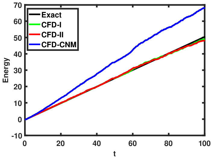
Refer to caption — Figure 1: Averaged energy evolution relationship ( $f(u)=0,g(u)=1$ ) with $\Delta t=1/20,h=1/10$

4 Numerical experiments

This section presents various numerical experiments in order to illustrate the energy-preserving property of the proposed fully-discrete schemes (3.4) and (3.16) with $l=1,2$ for the 1-dimensional nonlinear stochastic wave equation under the homogeneous Dirichlet boundary condition. We will compare the proposed numerical schemes with the following classical fully-discrete schemes based on

1. backward Euler-Maruyama (BEM) method ([15]) and compact finite difference method (2.3)

\left\{\begin{aligned} \mathbf{U}^{n+1}&=\mathbf{U}^{n}+\Delta t\mathbf{V}^{n+1},\\ \mathbf{V}^{n+1}&=\mathbf{V}^{n}+\Delta t\mathbf{A^{-1}D}\mathbf{U}^{n+1}-\Delta tF(\mathbf{U}^{n+1})dt+G(\mathbf{U}^{n})\mathbf{e}\boldsymbol{\Lambda}\Delta\boldsymbol{\beta}_{n},\\ \end{aligned}\right.

(4.1)

2. backward Euler-Maruyama (BEM) method ([15]) and discontinuous Galerkin finite element method (2.14)

\left\{\begin{aligned} U^{n+1}&=U^{n}+\Delta tV^{n+1},\\ V^{n+1}&=V^{n}+\Delta t\Delta_{h}U^{n+1}-\Delta tP_{h}f(U^{n+1})+P_{h}g(U^{n})\Delta W_{n},\end{aligned}\right.

(4.2)

3. semi-implicit Crank-Nicolson-Maruyama (CNM) method ([13, 25]) and compact finite difference method (2.3)

\left\{\begin{aligned} \mathbf{U}^{n+1}&=\mathbf{U}^{n}+\Delta t\frac{\mathbf{V}^{n}+\mathbf{V}^{n+1}}{2},\\ \mathbf{V}^{n+1}&=\mathbf{V}^{n}+\Delta t\mathbf{A^{-1}D}\frac{\mathbf{U}^{n}+\mathbf{U}^{n+1}}{2}-\Delta tF(\mathbf{U}^{n})+G(\mathbf{U}^{n})\mathbf{e}\boldsymbol{\Lambda}\Delta\boldsymbol{\beta}_{n},\\ \end{aligned}\right.

(4.3)

4. semi-implicit Crank-Nicolson-Maruyama (CNM) method ([13, 25]) and discontinuous Galerkin finite element method (2.14)

\left\{\begin{aligned} U^{n+1}&=U^{n}+\Delta t\frac{V^{n}+V^{n+1}}{2},\\ V^{n+1}&=V^{n}+\Delta t\Delta_{h}\frac{U^{n+1}+U^{n}}{2}-\Delta tP_{h}f(U^{n})+P_{h}g(U^{n})\Delta W_{n}.\end{aligned}\right.

(4.4)

For convenience, we denote numerical schemes (3.5), (3.6), (4.1) and (4.3) by CFD-I, CFD-II, CFD-BEM and CFD-CNM, respectively, in the case that the semi-discrete scheme is based on the compact finite difference method. Similarly, for the case that discontinuous Galerkin finite element method is applied in spatial direction, the numerical schemes (3.16) with $l=1,2$ , (4.2), (4.4) are denoted by DG-I, DG-II, DG-BEM and DG-CNM, respectively. The first and second examples (Subections 4.1 and 4.2) test the numerical approximation by simulating the stochastic wave equation with globally Lipschitz continuous coefficients. In Subection 4.3, numerical tests of the proposed fully-discrete schemes for the non-globally Lipschitz case are presented. In all the experiments, the expectation is approximated by taking average over 1000 realizations.

4.1 Stochastic wave equation with $f(u)=0$

Consider the following stochastic wave equation

\left\{\begin{aligned} &du=vdt,\\ &dv=\Delta udt+g(u)dW(t),&&(x,t)\in(0,1)\times(0,100]\end{aligned}\right.

(4.5)

with initial conditions $u(x,0)=0,v(x,0)=1$ . In this experiment, the diffusion coefficients are chosen as $g(u)=1$ , $g(u)=\sin(u)$ and $g(u)=u$ , which correspond to the additive noise case and multiplicative noise cases, respectively. In the sequel, we choose the orthonormal basis $\left\{e_{k}\right\}_{k\in\mathbb{N}+}$ and the corresponding eigenvalue $\left\{q_{k}\right\}_{k\in\mathbb{N}+}$ of $Q$ as

\displaystyle e_{k}=\sqrt{2}\sin(k\pi x),\quad q_{k}=\frac{1}{k^{6}}.

When $g(u)=1,$ it is known that the averaged energy of the exact solution grows linearly as time increases. The left hand picture of Fig. 1 plots the quantity $\frac{h}{2}\mathbb{E}[(\mathbf{V}^{n})^{\top}\mathbf{V}^{n}-(\mathbf{U}^{n})^{\top}\mathbf{A^{-1}D}\mathbf{U}^{n}]$ for CFD-I, CFD-II and CFD-BEM, and the right hand picture of Fig. 1 plots the quantity $\frac{1}{2}\mathbb{E}[\langle V^{n},V^{n}\rangle-\langle\Delta_{h}U^{n},U^{n}\rangle]$ for DG-I, DG-II and DG-BEM for $n=1,\ldots,N,$ in the case of the stochastic wave equation (4.5) with additive noise. Moreover, the reference straight line (black line) in Fig. 1 stands for the averaged energy evolution law of the exact solution, and has slope $\frac{1}{2}\sum_{k=1}^{N}q_{k}$ with $N=2000$ . It can be observed that the proposed schemes named CFD-I, CFD-II, DG-I and DG-II reproduce the linear growth of the averaged energy, but both CFD-BEM and DG-BEM do not. The numerical results coincide with the fact that the BEM method applied does not preserve the averaged evolution law of the linear stochastic oscillator (see [23]). Fig. 2 and Fig. 3 demonstrate the evolution of the discrete averaged energy for CFD-I, CFD-II, CFD-BEM, DG-I, DG-II and DG-BEM of the stochastic wave equation (4.5) with $g(u)=\sin(u)$ and $g(u)=u$ , respectively. We can see that the averaged energy in Fig. 3 grows faster than that in Fig. 2. Furthermore, it can be also checked that the proposed four schemes preserve perfectly the averaged energy evolution law, while CFD-BEM and DG-BEM fail.

4.2 Nonlinear stochastic wave equation with $f(u)=\sin(u)$

In this section, we consider the following nonlinear stochastic equation

\left\{\begin{aligned} &du=vdt,\\ &dv=\Delta udt-\sin(u)dt+g(u)dW(t),&&(x,t)\in(0,1)\times(0,100]\end{aligned}\right.

(4.6)

with $u(x,0)=0,v(x,0)=1$ , and take the cases $g(u)=1$ and $g(u)=\sin(u)$ into account.

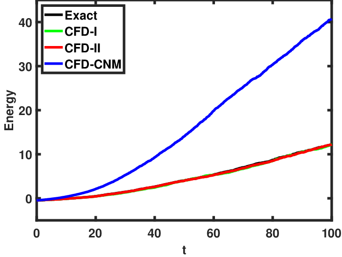
Figs. 4-5 present the evolution of discrete averaged energies for fully-discrete schemes named CFD-I, CFD-II, DG-I, DG-II, CFD-CNM and DG-CNM. From Fig. 4, it can be seen that averaged energies associated with numerical solutions of CFD-I, CFD-II, DG-I and DG-II grow linearly with the time raising, and coincide with the averaged energy of exact solution when the stochastic wave equation is driven by additive noise. Although the expected energies of CFD-CNM and DG-CNM also possess the linear growth property, the slope of blue lines is greater than the one of the reference black one, which means that CFD-CNM and DG-CNM could not inherit the averaged energy evolution law of the original nonlinear stochastic wave equation with additive noise. In the case of stochastic wave equation (4.5) driven by multiplicative noise, from Fig. 5 it also can be found the preservation of averaged energy of the proposed schemes, and the unpreservation of CFD-CNM and DG-CNM. The numerical results are consistent with the theoretical results. Fig. 6 displays the temporal approximation errors $\|u(T)-U^{N}\|$ against $N$ on log-log scale with $N=2^{\bf s},\,{\bf s}=3,4,5,6$ at time $T=1$ for multiplicative noise with $g(u)=\sin(u).$ We simulate the exact solution with the numerical one using a sufficiently small step size $\Delta t=2^{-11}.$ It can be observed that the slopes of six fully-discrete schemes are closed to 1 on the temporal convergence order.

4.3 Nonlinear stochastic wave equation with $f(u)=u^{3}$

In this subsection, we focus on the following nonlinear stochastic equation

\left\{\begin{aligned} &du=vdt,\\ &dv=\Delta udt-u^{3}dt+g(u)dW(t),&&(x,t)\in(0,1)\times(0,100],\end{aligned}\right.

(4.7)

subject to the initial conditions $u(x,0)=0,$ $v(x,0)=1$ . The diffusion coefficients are the same as those in Section 4.1, and the six fully-discrete schemes are chosen as same as those in Section 4.2. Note that the well-posedness of the nonlinear stochastic wave equation (4.7) with cubic nonlinearity and the considered diffusion coefficient can be obtained in [4, 7, 22].

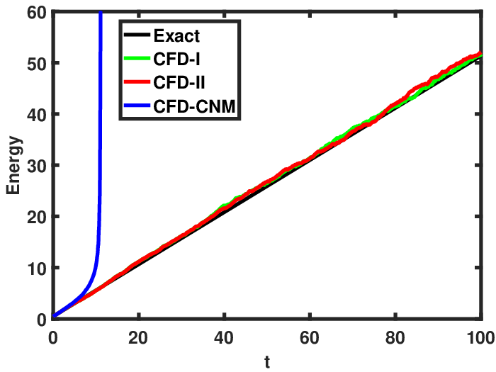
For the case of additive noise, Fig. 7 shows that the averaged energies of CFD-I, CFD-II, DG-I and DG-II grow linearly, and coincide with the averaged energy of the exact solution. However, the averaged energies of CFD-CNM and DG-CNM grow very fast and do not grow linearly, which fail to preserve the averaged energy evolution law of the original system. For the cases of multiplicative noise, i.e., the diffusion coefficients are chosen as $g(u)=\sin(u)$ and $g(u)=u$ , Figs. 8-9 also indicate that the four proposed schemes preserve the evolution of averaged energy, while the CFD-CNM and DG-CNM schemes do not, which coincide with theoretical analysis results, and Fig. 9 demonstrates clearly the effectiveness of the proposed fully-discrete schemes for simulating the nonlinear stochastic wave equation with multiplicative noise and non-globally Lipschitz continuous drift coefficient. In addition, it can be seen clearly that the averaged energy in Fig. 9 grows faster than that in Fig. 8. Compared with the reference line in Fig. 6 , it can be observed that the strong convergence order of six fully-discrete schemes is 1 in temporal direction.

5 Conclusion

In this paper, we propose fully-discrete schemes by the compact finite difference method or the interior penalty discontinuous Galerkin finite element method in space, the discrete gradient method and the Padé approximation in time, for solving the nonlinear stochastic wave equations driven by multiplicative noise. We prove that the proposed schemes preserve the discrete averaged energy evolution laws exactly. Numerical experiments confirm the theoretical analysis results. One future work is the study of the strong convergence analysis and the estimate of the strong convergence order for the proposed schemes, which is widely used to characterize the efficiency and accuracy of numerical method. Another future work is the numerical study of the nonlinear stochastic wave equations with non-globally Lipschitz nonlinearity, which is difficult to obtain the well-posedness and strong convergence order of numerical schemes.

Acknowledgements

This work is supported by National Natural Science Foundation of China (No. 11971470, No. 11871068, No. 12031020, No. 12022118).

References

[1] R. Anton, D. Cohen, S. Larsson, X. Wang, Full discretization of semilinear stochastic wave equations driven by multiplicative noise, SIAM J. Numer. Anal. 54 (2016) 1093-1119.
[2] D. Arnold, An interior penalty finite element method with discontinuous elements, SIAM J. Numer. Anal. 19 (1982) 742-760.
[3] L. Banjai, G. Lord, J. Molla, Strong convergence of a Verlet integrator for the semi-linear stochastic wave equation, arXiv: 2009.07710.
[4] V. Barbu, M. Röckner, The finite speed of propagation for solutions to nonlinear stochastic wave equations driven by multiplicative noise, J. Differential Equations 255 (2013) 560-571.
[5] S. Britt, E. Turkel, S. A. Tsynkov, High order compact time/space finite difference scheme for the wave equation with variable speed of sound, J. Sci. Comput. 76 (2018) 777-811.
[6] Y. Cao, L. Lin, Spectral Galerkin method for stochastic wave equations driven by space-time white noise, Commun. Pure Appl. Anal. 6 (2007) 607-617.
[7] P. Chow, Stochastic wave equations with polynomial nonlinearity, Ann. Appl. Probab. 12 (2002) 361-381.
[8] D. Cohen, S. Larsson, M. Sigg, A trigonometric method for the linear stochastic wave equation, SIAM J. Numer. Anal. 51(2013) 204-222.
[9] D. Cohen, L. Quer-Sardanyons, A fully discrete approximation of the one-dimensional stochastic wave equation, IMA J. Numer. Anal. 36 (2016) 400-420.
[10] J. Cui, J. Hong, L, Ji, L, Sun, Energy-preserving exponential integrable numerical method for stochastic cubic wave equation with additive noise, arXiv: 1909.00575.
[11] R. Dalang, D. Khoshnevisan, C. Mueller, D. Nualart, Y. Xiao, A minicourse on stochastic partial differential equations, Lecture Notes in Math. 1962, Springer-Verlag, Berlin, 2009.
[12] D. Deng, D. Liang, The time fourth-order compact ADI methods for solving two-dimensional nonlinear wave equations. Appl. Math. Comput. 329 (2018) 188-209.
[13] E. Hausenblas, Approximation for semilinear stochastic evolution equations, Potential Anal. 18(2003) 141-186.
[14] R. S. Hirsh, Higher order accurate difference solutions of fluid mechanics problems by a compact differencing technique, J. Comput. Phys. 19 (1975) 90-109.
[15] P. E. Kloeden, E. Platen, Numerical solution of stochastic differential equations, Appl. Math. (New York) 23, Springer-Verlag, Berlin, 1992.
[16] M. Kovács, S. Larsson, F. Saedpanah, Finite element approximation of the linear stochastic wave equation with additive noise, SIAM J. Numer. Anal. 48 (2010) 408-427.
[17] Y. Li, C. Shu, S. Tang, A discontinuous Galerkin method for stochastic conservation laws, SIAM J. Sci. Comput. 42 (2020) A54-A86.
[18] G. N. Milstein, Y. M. Repin, M. V. Tretyakov, Numerical methods for stochastic systems preserving symplectic structure, SIAM J. Numer. Anal. 40 (2002) 1583-1604.
[19] H. Moghaderi, M. Dehghan, A multigrid compact finite difference method for solving the one-dimensional nonlinear sine-Gordon equation, Math. Methods Appl. Sci. 38 (2016) 3901-3922.
[20] M. Y. Ongun, The Laplace adomian decomposition method for solving a model for HIV infection of CD4+T cells, Math. Comput. Modelling 53 (2011) 597-603.
[21] L. Quer-Sardanyons, M. Sanz-Solé, Space semi-discretizations for a stochastic wave equation, Potential Anal., 24 (2006) 303-332.
[22] H. Schurz, Analysis and discretization of semi-linear stochastic wave equations with cubic nonlinearity and additive space-time noise, Discrete Contin. Dyn. Syst. Ser. S 2 (2008) 353-363.
[23] A. H. Strømmen Melbø, D. J. Higham, Numerical simulation of a linear stochastic oscillator with additive noise, Appl. Numer. Math. 51 (2004) 89-99.
[24] X. Wang, An exponential integrator scheme for time discretization of nonlinear stochastic wave equation, J. Sci. Comput. 64 (2015) 234-263.
[25] J. B. Walsh, Finite element methods for parabolic stochastic PDE’s, Potential Anal. 23 (2005) 1-43.
[26] J. B. Walsh, On numerical solutions of the stochastic wave equation, Illinois J. Math. 50 (2006) 991-1018.

Energy-preserving fully-discrete schemes for nonlinear stochastic wave equations with multiplicative noiseJournal: *

Abstract

Keywords:

1 Introduction

2 Energy-preserving semi-discrete schemes in space

2.1 Semi-discrete scheme via the compact finite difference method

Theorem 2.1.

Remark 2.2.

2.2 Semi-discrete scheme via the interior penalty discontinuous Galerkin finite element method

Theorem 2.3.

Remark 2.4.

3 Energy-preserving fully-discrete schemes

Theorem 3.5.

Remark 3.6.

Remark 3.7.

4 Numerical experiments

4.1 Stochastic wave equation with f⁡(u)=0f(u)=0

4.2 Nonlinear stochastic wave equation with f⁡(u)=sin⁡(u)f(u)=\sin(u)

4.3 Nonlinear stochastic wave equation with f⁡(u)=u3f(u)=u^{3}

5 Conclusion

Acknowledgements

References

References

4.1 Stochastic wave equation with $f(u)=0$

4.2 Nonlinear stochastic wave equation with $f(u)=\sin(u)$

4.3 Nonlinear stochastic wave equation with $f(u)=u^{3}$