The HulC: Confidence Regions from Convex Hulls
Abstract
We develop and analyze the HulC, an intuitive and general method for constructing confidence sets using the convex hull of estimates constructed from subsets of the data. We present this method in the context of independent data. Unlike classical methods which are based on estimating the (limiting) distribution of an estimator, the HulC is often simpler to use and effectively bypasses this step. In comparison to the bootstrap, the HulC requires fewer regularity conditions and succeeds in many examples where the bootstrap provably fails. Unlike subsampling, the HulC does not require knowledge of the rate of convergence of the estimators on which it is based. The validity of the HulC requires knowledge of the (asymptotic) median-bias of the estimators. We further analyze a variant of our basic method, called the Adaptive HulC, which is fully data-driven and estimates the median-bias using subsampling. We show that the Adaptive HulC retains the aforementioned strengths of the HulC. In certain cases where the underlying estimators are pathologically asymmetric the HulC and Adaptive HulC can fail to provide useful confidence sets. We propose a final variant, the Unimodal HulC, which can salvage the situation in cases where the distribution of the underlying estimator is (asymptotically) unimodal. We discuss these methods in the context of several challenging inferential problems which arise in parametric, semi-parametric, and non-parametric inference. Although our focus is on validity under weak regularity conditions, we also provide some general results on the width of the HulC confidence sets, showing that in many cases the HulC confidence sets have near-optimal width.
Abstract
This supplement contains the proofs of all the main results in the paper.
1 Introduction
Estimation and uncertainty quantification are two of the most fundamental aspects of statistical analysis. The theory of point estimation is very well-studied starting from the principle of maximum likelihood estimation (Stigler, 2007; Pfanzagl, 1994; Lehmann and Casella, 1998). Relatively more recent frameworks of parametric efficiency (van der Vaart, 1998, Chapters 4–8) and semiparametric influence functions (Bickel et al., 1993) provide general methods of constructing good estimators. Uncertainty quantification, for instance, when testing a statistical hypothesis or constructing a confidence set, most often follows from studying the asymptotic distribution of the estimator. In many cases this approach requires estimating the asymptotic distribution of the estimator (properly normalized). Even in favorable cases, when this asymptotic distribution is mean zero Gaussian, one needs to further estimate the asymptotic variance of the estimator in order to construct a valid confidence set. As a consequence, in practice, methods which yield uncertainty quantification while using only a method for point estimation are often favored.
Generic techniques to obtain uncertainty quantification that do not require any more than the estimation method are the bootstrap and subsampling (Efron, 1979; Politis and Romano, 1994; Shao and Tu, 1995; Hall, 1992). The bootstrap however requires that the estimator be Hadamard differentiable; see Dümbgen, 1993 and Shao and Tu, 1995. Subsampling is more general, but requires knowing the rate of convergence of the estimator. Bertail et al., 1999 provides a scheme to estimate the unknown rate of convergence, but this method cannot estimate the slowly varying components of the rate (such as factors); see Sherman and Carlstein, 2004 for details.
In this paper, we propose a new method, the HulC (Hull based Confidence) that does not require variance estimation and is applicable in many examples where the bootstrap and subsampling are not. The HulC does not require knowing the rate of convergence of the estimator. In many cases, the HulC does not involve any tuning parameters. Besides being asymptotically valid, the HulC is eventually finite sample meaning that the coverage is exact for all samples of size for some finite . Throughout the paper, we restrict ourselves to independent data. Although applicable for dependent data, HulC for dependent data is beyond the scope of the current paper and will be dealt with elsewhere.
The basis for the HulC is an assumption that the estimators on which it is based are not pathologically asymmetric: their distributions do not place all their mass to one side of the target parameter. We measure the asymmetry in terms of the median bias of the estimator. This makes the method widely applicable and easy to use. Our method has some similarity to the typical values approach of Hartigan, 1969; Hartigan, 1970. See, in particular, point 5 in Section 7 of Hartigan, 1970. The work of Ibragimov and Müller, 2010 also uses estimators computed on a fixed number of splits of the data as we do and combines them via a -statistic to obtain an asymptotically valid confidence interval; also, see Lam, 2022. We note that, unlike ours, this approach relies heavily on the asymptotic normality of a properly normalized estimate.
Mean unbiasedness is a popular criterion for good estimators and mean bias reduction is well-studied in the statistics literature (Firth, 1993; Kosmidis and Firth, 2009; Kim, 2016). However, as noted in Pfanzagl, 2017 the fact that an estimator is mean unbiased does not naturally aid in uncertainty quantification. In contrast, median unbiasedness implies that the estimator is equally likely to underestimate and overestimate the target of interest. As will be shown in this article, this property can lead to a simple method for constructing confidence intervals. Median unbiasedness and median bias reduction are not as widely known as the mean unbiasedness and mean bias reduction, but we will develop their implications for inference. We refer the reader to Pfanzagl, 1994 for details regarding median unbiased estimation and to Kenne Pagui et al., 2017; Kosmidis et al., 2020 for median bias reduction methods in parametric models.
Inspired by the practical success of resampling methods like the bootstrap and subsampling, the HulC directly exploits our relatively strong understanding of point estimation to address challenging inferential problems. As with these methods, the width of the intervals we construct is naturally related to the accuracy of the underlying estimators, i.e. the HulC based on a very accurate estimator will lead to small confidence sets. On the other hand, in contrast to these methods, the HulC uses sample-splitting to avoid strong regularity conditions, and its validity relies instead on a relatively mild assumption. This follows a line of recent work by the authors (for instance, Wasserman et al., 2020; Chakravarti et al., 2019; Rinaldo et al., 2019), and more classical work by Bickel, 1982, where sample-splitting eases the challenges of statistical inference, often at a surprisingly small price.
The remainder of this article is organized as follows. In Section 2, we describe our assumptions and the HulC method for constructing confidence regions for univariate and multivariate parameters. We compare the proposed confidence interval to Wald confidence intervals based on asymptotic Normality in terms of their widths. We also compare to the bootstrap and subsampling in terms of applicability. In Section 3, we discuss the applicability of the HulC to some standard examples where limiting distributions are well-understood but constructing valid confidence sets can still be challenging; the examples we consider include mean and median estimation, Binomial proportion estimation, and parameter estimation in exponential families. Our method involves an assumption on the median bias of the estimators under consideration. In Section 4, we describe the Adaptive HulC which estimates the median bias using subsampling. Interestingly, in contrast to directly using subsampling for constructing a confidence set, the Adaptive HulC does not require knowledge of the rate of convergence. In Section 5, we provide some applications of the Adaptive HulC to nonparametric models including shape constrained regression. In Section 6, we provide an extension, called the Unimodal HulC, based on the assumption of unimodality. Between our median bias assumption and unimodality assumption, we believe that many challenging confidence set construction problems based on independent observations are solved. In Section 7, we briefly discuss the application of HulC for multivariate parameters/functionals. Finally, in Section 8, we summarize the article and discuss some future directions. Throughout the article, we focus on the pointwise validity (as in Politis and Romano, 1994) of our confidence region, where we treat the distribution of the data as fixed, as the sample size increases. Some preliminary results on uniform validity of HulC are presented in Kuchibhotla et al., 2023.
The proofs of all the main results are provided in the supplementary material. Section S.1 provides a discussion on the application of Bonferroni inequality with Wald interval, supplementing HulC method for multivariate parameters in Section 7. The sections and equations of the supplementary file are prefixed with “S.” and “E.”, respectively, for convenience. We provide the code to reproduce the figures in the paper, including an implementation of our methods in R together with Jupyter notebooks illustrating their application at https://github.com/Arun-Kuchibhotla/HulC.
2 The HulC: Hull based Confidence Regions
In this section, we describe the HulC and compare it to classical asymptotic normality based confidence intervals. We present several results for the HulC, and in order to aid readability we provide a brief roadmap here:
- 1.
Focusing first on univariate parameters, in Theorem 1, we show that when the median bias of the estimators is known to be at most the HulC (as described in Algorithm 1) has guaranteed coverage of at least . We also show that, under some mild additional conditions, if the underlying estimators have median bias exactly then the HulC has coverage exactly .
- 2.
In Proposition 1, we investigate properties of a (slightly) conservative variant of the HulC, showing that the HulC when provided with the asymptotic median bias still ensures finite-sample coverage, for sufficiently large sample sizes. This setting is practically useful because in many cases we know the limiting distribution of our estimates is normal (say) and in these cases the asymptotic median bias is known to be 0.
- 3.
- 4.
In (25) and (26), we provide two simple analyses of the width of the HulC intervals. In (25) we show that in the classical setting where the estimates have an asymptotic normal distribution, the width of the HulC interval is the same as that of the corresponding Wald interval up to a factor of . In (26), we show that under much more generality the HulC based on splits yields a variance-sensitive confidence interval whose expected width is upper bounded by , where is the standard deviation of the estimators on which the HulC is based.
2.1 HulC for univariate parameters
Suppose is a parameter or functional of interest. Let be independent random variables from some measurable space . For , let be independent estimators of . These can be obtained by splitting the data into batches and computing an estimate from each batch. Formally, let be a (random) partition of into subsets. For , let be the estimator computed on -th batch of observations . Define the median bias of the estimator for as
| (1) |
where for any . From the definition, it is clear that lies in . Using the independence of the estimators , we obtain the following result (proved in Section S.2 of the supplementary material).
Lemma 1.
If are independent random variables and
| (2) |
then
Observe that in general depends on , the distribution of the data as well as the batch sizes , …, . For simplicity, we do not index with these quantities. Lemma 1 provides a two-sided confidence interval with a bound on the miscoverage probability. It is easy to also obtain one-sided confidence intervals with explicit bounds on miscoverage. For instance, if there exists a such that for all , then .
An estimator is said to median unbiased for if (Pfanzagl, 1994). It is worth noting that median unbiasedness does not imply that the estimator is symmetric. The non-strict inequality in the definition (1) is important: it allows for and to be equal to or be larger than . This is useful in cases where is on the boundary or has a discrete distribution and puts non-zero mass at . An estimator based on observations is asymptotically median unbiased if . One of the prominent examples of asymptotically median unbiased estimators is the class of asymptotically normal estimators; some of these are described in Section 3. A simple example with non-zero asymptotic median bias is the estimation of , where is the mean of i.i.d. random variables . The estimator has an asymptotic median bias of when as shown in Section 3.5. (Here denotes the chi-square random variable with degrees of freedom 1.)
For any and , set the upper bound on the miscoverage probability from Lemma 1 as
| (3) |
If is known, then choosing such that , we conclude that
In words, the smallest rectangle (interval) containing independent estimators of has a coverage of at least 11 1 Throughout this paper we use the phrase “asymptotically valid” (or “valid”) to indicate that the coverage is asymptotically (or finite-sample) at least . When the coverage is exactly we indicate this by the phrase “asymptotically exact” (or simply “exact” in the finite-sample setting).. The smallest interval containing estimators is their (convex) hull and hence we call this interval HulC (Hull based Confidence) interval. Because is an integer, decreases in steps as changes over positive integers and this can lead to conservative coverage i.e., miscoverage probability strictly less than as there may not exist an integer such that . This issue can be resolved easily by randomizing the choice of . Formally, we generate a random variable from the uniform distribution on and set
| (4) |
If , then . Most often is unknown. This issue will be resolved in Section 4 where we show how to estimate .
Algorithm 1 gives the steps to find a randomized confidence interval with coverage when the median bias is known.
| (5) |
There are no restrictions on the input in Algorithm 1 except that it produces an estimate with median bias bounded by . Its rate of convergence and variance play a role only in the width properties of the resulting confidence interval, not in the validity guarantee. A better estimator will lead to a smaller confidence interval. Here are two examples of the estimation procedure :
- •
If are identically distributed and , then one can take In general, the median bias of the sample mean is unknown, but typically tends to zero as . If the observations are symmetrically distributed around , then
- •
If are random variables generated from a parametric model that belongs to the parametric family , then one can take as the maximum likelihood estimator (MLE) of based on the observations . Under standard regularity conditions, MLE has an asymptotic normal distribution and hence the median bias of converges to zero.
The following result (proved in Section S.3 of the supplementary material) establishes that the confidence interval from Algorithm 1 has a coverage of at least .
Theorem 1.
If are independent random variables and the estimation procedure in Algorithm 1 returns estimates that have a median bias of at most , then the confidence interval returned by Algorithm 1 satisfies
| (6) |
Further, if , for all , and the estimation procedure in Algorithm 1 returns estimates that have a median bias of exactly , then
| (7) |
In Algorithm 1, it is implicitly assumed that defined in step 2 is smaller than the sample size so that the estimation procedure can be applied on splits of the data. Recall from (3) and that is the smallest integer such that It is easy to prove that is an increasing function of and hence we obtain that . Therefore, satisfies
| (8) |
Here , for any real , denotes the smallest integer larger than . It is easy to verify that, as . Figure 1 shows the plot of as varies from to and varies between . The right panel of Figure 1 shows the values of for some choices of and . In the favourable case of , and for the usual choices of , the number of independent splits required is about 5, a feasible choice for any reasonable sample size.
| 0.15 | 0.1 | 0.05 | |
|---|---|---|---|
| 0 | 4 | 5 | 6 |
| 0.05 | 4 | 5 | 6 |
| 0.1 | 5 | 5 | 7 |
| 0.15 | 5 | 6 | 7 |
| 0.2 | 6 | 7 | 9 |
| 0.25 | 7 | 9 | 11 |
| 0.3 | 9 | 11 | 14 |
| 0.35 | 12 | 15 | 19 |
| 0.4 | 19 | 22 | 29 |
2.2 HulC when asymptotic median bias is known
Algorithm 1 requires knowledge of the median bias of the estimators. In some settings, estimation procedures can be constructed so as to ensure median unbiasedness (i.e., ). When , . These examples are discussed in Section 3.
Because is a piecewise constant function in , we do not need to know exactly. This observation implies that for estimators that are asymptotically symmetric around , one can take to be zero in Algorithm 1 and still retain (asymptotic) validity. Formally, if as , then the convex hull of estimators has an asymptotic coverage of at least . Furthermore, the convex hull is eventually finite sample valid, meaning that there is a sample size such that the coverage is at least for all . Now, we provide more details.
Proposition 1 proved in Section S.4 of the supplementary material formally establishes that is a piecewise constant function of (as illustrated in Figure 1).
Proposition 1.
For and , if
| (9) |
then Moreover, if
| (10) |
then .
Remark 2.1 Note that the right hand side of (9) is non-zero if and only if in (4). In a typical application, one would take as the hypothesized (or asymptotic) value of the median bias and is the true median bias. Hence, the right hand side of (9) can be computed exactly for any user choice of . As a practical matter, the user can change by a tiny amount to increase the right hand side of (9). In the most common setting of asymptotic normality, , and consequently the requirement becomes more relaxed as in (10); this relaxation stems from the fact that has zero first derivative at . Using the definition of Lambert function, the fact that , and that , the requirement (10) can be shown to be implied by
| (11) |
where represents the principal branch of the Lambert function. Figures S.1 and S.2 show the behavior of the right hand sides of (9) and (11) for various values of and .
Recall from the calculation surrounding (3) that the smallest interval containing estimators has a coverage of at least if the estimators have a median bias of at most . Proposition 1 implies that one need not know the median bias of the estimators exactly in order to find . Suppose the estimators have a known asymptotic median bias of . Recall defined in (4). Proposition 1 implies that for every satisfying there exists such that for all
| (12) |
Inequality (12) is obvious from Lemma 1 with estimators. Proposition 1 along with asymptotic median bias of implies that for . The threshold sample size depends on how fast converges to zero and how big the right hand side of (9), (10) are. The coverage guarantee (12) can be compared to the coverage guarantee for Wald, bootstrap, and subsampling intervals. None of these intervals have a guarantee of at least coverage even for large sample sizes; the coverage only converges to with sample size.
To understand how depends on , we consider bounds on which use traditional Berry–Esseen bounds. In most cases including parametric and semiparametric models, Berry–Esseen type bounds are available that provide bounds of the form,
| (13) |
where is the number of observations in the -th split of the sample based on which is computed. Here is a constant that depends on the true distribution of the data. (If is the sample mean, then can be bounded in terms of the skewness of the random variables .) For results of this type, see Pfanzagl, 1971; Pfanzagl, 1973a, Bentkus et al., 1997; Bentkus, 2005, and Pinelis, 2017. (In semi/non-parametric models as in Zhang and Liang, 2011 and Han and Kato, 2022, the rate of convergence may be slower than .) In this case, assuming (i.e., data is split approximately equally into many samples), we get that,
| (14) |
Note that this conclusion requires a weaker bound than the one in (13) because we only care about in (13). For example, in case of the sample mean, if the observations are symmetric around the population mean, then irrespective of any moment assumptions, but a general Berry–Esseen bound (13) need not hold true without additional moment assumptions. If we take to be the set of all strictly increasing functions and is the class of all continuous distributions with , then can also be bounded as
| (15) |
This follows from the fact that for all strictly increasing functions . Allowing for arbitrary increasing transformations may result in better normal approximations in many cases. Classical examples include the Fisher’s z-transformation for the correlation coefficient and Anscombe’s arcsine transformation for Binomial random variable; see Borges, 6970; Gebhardt, 1969; Borges, 1971; Efron, 1982 for some examples. Because symmetric distributions belong to and the standard normal distribution belongs to it, the right hand side of (15) is always better (i.e., smaller) than the bound attained by (13). Moreover, if has zero median, then the right hand side of (15) is zero but (13) can result in a constant order upper bound.
If inequality (14) holds true, then the requirement (11) holds if
| (16) |
This equivalence (16) follows from inequality (8) for . The right hand side of (16) can be as large as even for small values of as shown in Figure S.2.
By making use of an Edgeworth expansion, estimators with smaller median bias can be constructed via median bias reduction (Pfanzagl, 1973b; Kenne Pagui et al., 2017). Pfanzagl, 1973b provides a general recipe for constructing estimators with a median bias of for any . Kenne Pagui et al., 2017 yields estimates that satisfy . In this case, for some constant and hence, requirement (16) can be relaxed to
The reduction in median bias, hence, leads to a smaller threshold sample size after which our intervals are finite-sample valid.
The above argument for asymptotically median unbiased estimators implies that the smallest interval containing many independent estimators of has a finite sample coverage of at least after a sample size of . This, however, does not imply coverage validity for the confidence interval returned by Algorithm 1. This happens because with non-zero probability Algorithm 1 uses estimators. The following result proves upper and lower bounds on the miscoverage of the confidence interval returned by Algorithm 1 with whenever the estimation procedure has a median bias of converging to as sample size diverges to infinity. For simplicity, the result is stated only for asymptotically median unbiased estimators, i.e., . See Remark 2.2 and the proof of Theorem 2 for upper and lower bounds on true coverage when Algorithm 1 is applied with when the estimators has a median bias of at most .
Recall that is the confidence interval returned by Algorithm 1 when it is applied with as the median bias parameter. Theorem 2 below is proved in Section S.5.
Theorem 2.
Suppose are independent random variables. If the estimation procedure returns estimators that have a median bias of at most , then
| (17) |
Furthermore, if for all and all have the same median bias of , then
| (18) |
Note that the conditions of same median bias and same probability of undercoverage are trivally satisfied if all of the batches contain the same number of observations and all the observations are independent and identically distributed.
Remark 2.2 In Section S.5, we also consider the case when is not necessarily 0. If the finite-sample median bias of the estimation procedure is close to (rather than zero), then
Further, if and the estimators all have the same median bias , then
These two inequalities imply that if , then converges to .
Remark 2.3 The main conclusion of Theorem 2 is that Algorithm 1 can be used with and it retains asymptotic validity for large sample sizes if the estimation procedure produces asymptotically median unbiased estimators.
Theorem 2 is a finite sample result characterizing explicitly the effect of misspecifying in Algorithm 1. The misspecification of is measured by how far the median bias of the estimators is from , the asymptotic median bias. To illustrate Theorem 2, consider the setting under which (14) holds true. Theorem 2 along with (14) implies that,
| (19) |
In case an estimation procedure with reduced median bias is employed in Algorithm 1, then we get for some constant and hence, Theorem 2 yields
| (20) |
Theorem 2 (and the conclusions (19), (20)) can be compared to the guarantees offered by classical confidence intervals constructed based on the assumption of asymptotic normality. Under a bound like (13), such confidence intervals only satisfy
| (21) |
In other words, the coverage of differs from by a quantity of order and can significantly miscover if . The same comment also applies to the bootstrap and subsampling confidence intervals. Confidence intervals obtained by various methods are often compared in terms of the rate of convergence in (21). In parametric models or, more generally, cases where is estimable at an rate, confidence intervals which attain a rate of in (21) are called first-order accurate, those that attain a rate of are called second-order accurate and so on. Asymptotic normality based Wald confidence intervals are usually first-order accurate. Bootstrap confidence intervals can be constructed to be second-order accurate (Hall, 1986; Hall, 1988; Mammen, 1992). Subsampling intervals can also be constructed to satisfy second-order accuracy (Bertail and Politis, 2001). In contrast, the HulC readily obtains second-order accuracy and is valid even if converges to zero. Further, if we use an estimator with reduced median bias, the HulC is sixth-order accurate; see (20). Another important difference is that the HulC attains relative accuracy (i.e., is small) instead of absolute accuracy as in (21). In the problem of mean estimation, some results for relative accuracy of Wald confidence intervals are available using self-normalized large deviation techniques (Shao, 1997; Jing et al., 2003). To our knowledge, such refined results are unavailable for a large class of -estimators.
2.3 Comparison with Wald confidence intervals
In this section we show that our intervals have lengths close to those of the Wald intervals. In order to facilitate this comparison, we assume in this section that slowly as a function of . Let and . Suppose that
| (22) |
as and for all . Under this assumption, if is a consistent estimator , then the Wald confidence interval is given by where is the -th quantile of the standard Gaussian distribution. The scaled width of this confidence interval is given by This converges in probability to . From the properties of the normal distribution, it follows that as . See, for example, Proposition 4.1 of Boucheron and Thomas, 2012. Hence, the width of the Wald confidence interval is asymptotically equal to as and .
To compare this width to the width of the HulC, for simplicity, we treat as a fixed (i.e., non-stochastic) value and assume that is a multiple of so that each split has many observations. Assumption (22) implies that for Because the estimators are independent and , we get that the convergence is joint for all the estimators . Recall that our confidence interval is the smallest rectangle (interval) containing these estimators and hence
| (23) |
Joint asymptotic convergence of the estimators implies that
| (24) |
where is a Gaussian random vector with mean zero and a diagonal covariance matrix with all diagonal entries equal to . This shows the first difference in widths. Unlike the classical Wald confidence intervals, the width of our confidence interval does not degenerate after scaling by ; the width after proper scaling converges weakly to a non-degenerate distribution. Using (24), we can control of the width of our confidence region in terms of the width of the convex hull of many independent mean zero Gaussian random variables. Because ’s are symmetric around zero,
The last equality here holds as and follows from Theorem 1.2 of Kabluchko and Zaporozhets, 2019 (and the discussion before that theorem). Therefore, the width of our confidence interval is asymptotically From inequalities (8), we know that and are of order ; note that under asymptotic normality, we can take . Hence, the width of our confidence interval is asymptotically
| (25) |
This implies that the ratio of the expected width of our confidence interval to that of the Wald interval is approximately equal to . This is always larger than , and grows very slowly as . For , this ratio ranges between and . In a way, this is the price to pay for the generality of the confidence interval. While the Wald confidence interval makes complete use of asymptotic normality, our confidence interval only makes use of the fact that its median is zero; we do not even make use of symmetry.
Unlike the Wald confidence interval, the HulC does not explicitly or implicitly estimate the variance of the estimator but its width as given in (25) adapts to the unknown standard deviation . The calculation shown above uses asymptotic arguments, but some simple bounds can be obtained using no more than two moments for . Observe from (23) that
| (26) |
Assuming convergence in mean square of to a distribution with mean zero and variance , we get that the expected width is asymptotically bounded by . This calculation does not require convergence to Gaussianity and shows that the width of our confidence interval, in general, adapts to the standard deviation of the estimators. The calculation (26) can be significantly improved if the estimators are known to have higher moments. In the first inequality of (26) we only use second moment Jensen’s inequality. Replacing the second moments by -th moment here will yield instead of in the last line of (26).
Transformed Parameters.
In contrast to Wald intervals, the HulC interval is equivariant to monotone transformations, assuming that the estimators are equivariant under monotone transformations. It is worth noting that the validity of our confidence interval does not require any smoothness conditions on the transformation In comparison, the delta method requires continuous differentiability of .
2.4 Numerical Comparisons
2.4.1 Simple Linear Regression
Figure 2 shows the coverage and width of the 95% HulC interval (obtained from Algorithm 1 with ) and the Wald interval from ordinary least squares linear regression. The simulation setting is as follows: for , independent observations are generated from
| (27) |
For , observations follow the standard linear model and for , observations do not follow a linear model with non-linear mean function and a heteroscedastic error variable. With , misspecification from linear conditional expectation and homoscedasticity increase. We define the estimator and target as and , where
Here represents the expectation when are generated from (27). Note that need not be equal to for . By Monte-Carlo approximation of with samples, we have and . The Wald interval in this case is obtained using the sandwich variance estimator as in Buja et al., 2019.
2.4.2 Multiple Linear Regression
Figure 3 provides an illustration when the estimator is obtained from multiple linear regression. The setting for Figure 3 is as follows: for , independent observations are generated from , where and is generated according to the following law: , , , and . Here are independent of and . This is also a misspecified linear regression model and is taken from Kuchibhotla et al., 2021. Our estimator and target are defined as
where and represent the last 5 coordinates of and respectively. With Monte Carlo approximation of , we found that . For level , the HulC (with ) requires splitting the data into approximately 5 parts. This implies that for a sample of size , each part only has 4 observations and one cannot fit uniquely a linear regression estimator because the model has 6 covariates. Interestingly, when we just use the output from R function lm(), the HulC still covers the true with required confidence because in this case lm() simply ignores the last 2 covariates.
2.4.3 Quantile Regression
In the previous examples of simple and multiple regression both bootstrap and subsampling are well-known to be consistent and their width matches that of Wald interval as the sample size diverges. In this subsection, we consider the example of quantile regression where the theory can be a lot more subtle. We restrict ourselves to the case of quantile regression with one covariate and no intercept, i.e., with data , the estimator is given by
This is a univariate M-estimation problem with a convex objective function and the results of Kuchibhotla, 2021 imply that is asymptotically median unbiased for the population parameter without requiring any assumptions on the conditional distribution of given . On the other hand, asymptotic normality of requires existence of the conditional density of given ; see Knight, 1998; Knight, 1999; Knight, 2008 for details. Further, if the conditional density of given does not exist, then the rate of convergence depends on the smoothness properties of the conditional distribution function. For our discussion, we focus on a particular example discussed in Example 1 of Knight, 1999.
Suppose are independent and identically distributed random vectors obtained via
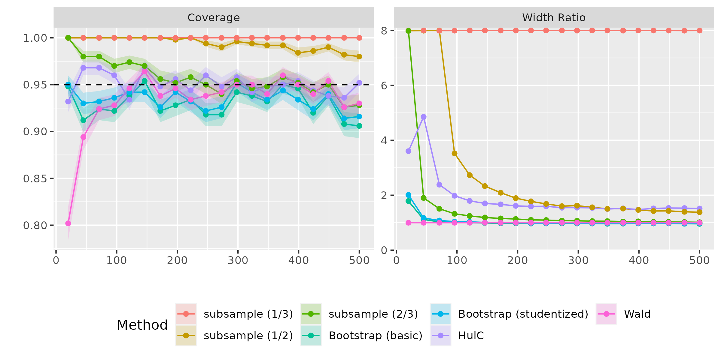
Theorem 1 (and Example 1) of Knight, 1999 imply that converges in distribution to a non-normal distribution defined by a minimization problem. Section 3 of Knight, 1999 shows that bootstrap is consistent for this problem if and only if (or equivalently, when the limiting distribution is normal). Subsampling is also not readily applicable because the rate of convergence of the estimator is unknown apriori. But subsampling with estimated rate of convergence as in Bertail et al., 1999 is applicable. We compare the performance of HulC , and subsampling with estimated rate of convergence with three different choices of subsample sizes (, , and ) across different and different sample sizes . (It is worth mentioning here that HulC does not involve any tuning parameters where as subsampling with estimated rate of convergence includes more than 10 tuning parameters other than the subsample size.) Figure 4 shows the performance of these procedures based on 200 Monte Carlo replications for each sample size and each .

3 Applications to standard problems
In this section, we present some simple applications including mean estimation, median estimation, and parametric exponential models. In parametric and semi-parametric models, regularity conditions and efficiency theory implies the existence of estimators which when centered at the target have an asymptotic mean zero Gaussian distribution. In these cases, often one can modify the estimators to ensure reduced median bias. For some examples of (approximately) median-unbiased estimators, see Birnbaum, 1964; John, 1974; Pfanzagl, 1970a; Pfanzagl, 1970b; Pfanzagl, 7172; Pfanzagl, 1979; Hirji et al., 1989; Andrews and Phillips, 1987; Kenne Pagui et al., 2017.
In all the examples in this section, we assume that the batch sizes are all the same, i.e., . This can be trivially achieved by ignoring less than observations, if necessary.
3.1 Mean estimation
Suppose are independent real-valued random variables with a common mean . Consider the problem of constructing a confidence interval for . Note that the random variables need not be identically distributed. If the random variables have a finite second moment and satisfy the Lindeberg condition, then the sample mean satisfies where . This implies that the estimator is asymptotically median unbiased and Algorithm 1 with yields an asymptotically valid confidence interval for . In this case, Wald intervals are also asymptotically valid.
The setting becomes more interesting when we consider random variables with less than two finite moments. In this case, the limiting distribution of is known to be a stable law and its rate of convergence also changes depending on the tail decay of the random variables. If the random variables satisfy
| (28) |
then the limiting stable law of is symmetric around zero (see, for instance, Theorem 9.34 in Breiman, 1992). In this special case, Algorithm 1 continues to provide asymptotically valid confidence intervals, while Wald intervals and the bootstrap are known to fail for ; see, for example, Athreya, 1987 and Knight, 1989. In particular, if the underlying distributions are all symmetric around the mean , then without any moment assumptions the confidence interval returned by Algorithm 1 is finite sample valid. It is worth noting that subsampling (Romano and Wolf, 1999) is still applicable in the case of infinite variance.
If the assumption (28) does not hold true, then the limiting stable law is not symmetric and the asymmetry depends on the gap between the left and right hand side quantities in (28). In this case, the median bias of the limiting distribution is not readily available and the methods presented in previous sections are not applicable. This can be resolved using the Adaptive HulC which we describe in Section 4.
3.2 Median estimation
Suppose are independent real-valued random variables with common median . Consider the problem of constructing a confidence interval for . The usual estimator for the population median is the sample median. Set . If the average distribution function has a derivative bounded away from zero at , then it is known (Sen, 1968) that where . Here is the derivative of at . There are several classical methods for constructing confidence intervals for including Wald’s, quantile or rank based intervals. Wald confidence intervals in this case require estimating of the density at and the quantile based intervals require choosing the appropriate quantiles for end points. Unlike the Wald interval, the quantile based intervals are finite sample valid (Lanke, 1974). Because the limiting distribution is mean zero Gaussian, the HulC applies and yields an asymptotically valid confidence interval.
Once again the setting becomes interesting when the underlying distributions do not satisfy the conditions for normality. For example, if the density is not bounded away from zero at the common median , then the limiting distribution of is not Gaussian and hence Wald as well as bootstrap intervals break down. The limiting distribution in this case is explicitly described in Knight, 1998. In this case, the rate of convergence of the median depends on how fast the density decays to zero as approaches . When the population median is unique, the sample median computed based on odd number of observations is known to be median unbiased (Desu and Rodine, 1969). This observation implies that Algorithm 1 with yields a finite sample valid confidence interval for if each has an odd number of observations (which can be trivially ensured). In fact, with any given number of observations (even or odd), an estimator that randomly (equally likely) chooses between the -th order statistic and -th order statistic is median unbiased for as shown in Section 4 of Desu and Rodine, 1969.
3.3 Binomial distribution
Consider for some . The problem of constructing confidence intervals for is a well-studied problem with focus on coverage as changes with the sample size (Brown et al., 2002). It is well-known that, when properly normalized, the limiting distribution of Binom as changes from a Gaussian to a Poisson distribution depending on whether or . Because of this change, the Wald confidence intervals can undercover when is small relative to the sample size (Brown et al., 2001). We will now consider the coverage properties of the HulC when using the sample proportion as an estimator for . For any set , Theorem 10 of Doerr, 2018 shows that whenever , the estimator has a median bias of at most . Theorem 1 of Greenberg and Mohri, 2014 yields this result for . For a more precise result, see Lemma 8 of Doerr, 2018. Hence, Algorithm 1 with yields finite sample coverage of at least for all ; here represents the minimum number of observations in each split of the data. Because , we get finite sample coverage validity even for . Note that the binomial distribution is not approximately normal in this case.
Allowing for some modifications of either the estimator or the final confidence set, we can obtain finite sample coverage for all . Firstly, note that the HulC interval from Algorithm 1 with will always cover the true median of the estimators. With the proportion estimator , the HulC interval from Algorithm 1 with with a probability of at least will contain the median of where for all . Hamza, 1995 proves that
| (29) |
Therefore, if represents the confidence interval from Algorithm 1 with , we get that for all ,
This is a modification of confidence interval returned by Algorithm 1 but uses the classical binomial proportion estimator. If we modify the estimator, then no changes are required in Algorithm 1 with to obtain a finite sample coverage. Because the binomial distribution has a monotone likelihood ratio, the results of Pfanzagl, 1970a; Pfanzagl, 7172 can be applied to obtain a median unbiased estimator of . It might be worth noting here that binomial distribution being discrete, any median unbiased estimator has to be randomized; see page 74 of Pfanzagl, 1994 for a discussion. The exact median unbiased estimator of Pfanzagl, 1970a; Pfanzagl, 7172 is computationally intensive. A simpler estimator for with reduced median bias can be obtained from Hirji et al., 1989, and Kenne Pagui et al., 2017. These works discuss binary regression and estimating a binomial proportion is the special case when there are no regressors except for an intercept. Hamza, 1995 also proves that (29) holds true for replaced by . This implies that the confidence interval from Algorithm 1 inflated by also has a finite sample coverage of at least for every .
3.4 Exponential families
Lehmann, 1959 provide median unbiased estimators in monotone likelihood ratio and exponential families with a Lebesgue density. Extending this work, Pfanzagl, 1979 provides an algorithm to construct an exactly median unbiased estimator for every sample size in a full rank exponential family, even in the presence of nuisance parameters. Pfanzagl, 1979 considers a more general parametric model than exponential families; see Read, 2004. A related result for exponential families is also obtained in Brown et al., 1976. For brevity, we will not describe this algorithm here and refer to the papers mentioned above; also, see Cabrera and Watson, 1997 for some computational methods. With such an estimator, the HulC can be applied with to obtain a finite sample valid confidence interval.
3.5 Squared mean estimation
Suppose are independent random variables with common mean and common variance . Consider the estimation of . A natural estimator of is , the square of the sample mean. The asymptotic distribution of depends on the true mean and the population variance:
| (30) |
There are two aspects to consider here. First, the rate of convergence changes from to as changes from non-zero to zero. Second, the limiting distribution of becomes one-sided for and this implies that the estimator has an asymptotic median bias of for . The first aspect is not an issue for Algorithm 1, but the second aspect renders Algorithm 1 useless for close to zero because it would require nearly infinite many splits of the data. Alternatively, for each subset of the data, consider the -statistic estimator
| (31) |
It readily follows that for all , unlike which is biased for close to zero. Once again has different limiting distributions depending the magnitude of . Specifically,
| (32) |
The rate of convergence changes between and , but now the limiting distribution has median bias bounded away from zero. It may be worth pointing out that the limiting distribution in general would be a mixture of normal and Chi-square as becomes close to zero. We can prove the following result on the median bias of that is uniform over all . The proof in Section S.7 can be easily extended to accommodate non-identically distributed observations expect for common mean and variance.
Proposition 2.
Suppose are independent and identically distributed. Then for any and , the median bias of is bounded by
| (33) |
Note that the first term on the right hand side of (33) can be computed given without the knowledge of and . Further, the last three terms of (33) all disappear as whenever certain moments of are bounded away from and . Exact computation for some sample sizes shows that the supremum in the first term in (33) is attained at and equals . Hence, Algorithm 1 can be applied with and the estimator to attain an uniformly valid asymptotic confidence interval for . It is worth pointing out that the resulting confidence interval is adaptive in its width as approaches zero, i.e. the expected width of the HulC interval scales as when is close to 0, and as when is large. This follows from the fact that has an adaptive rate of convergence.
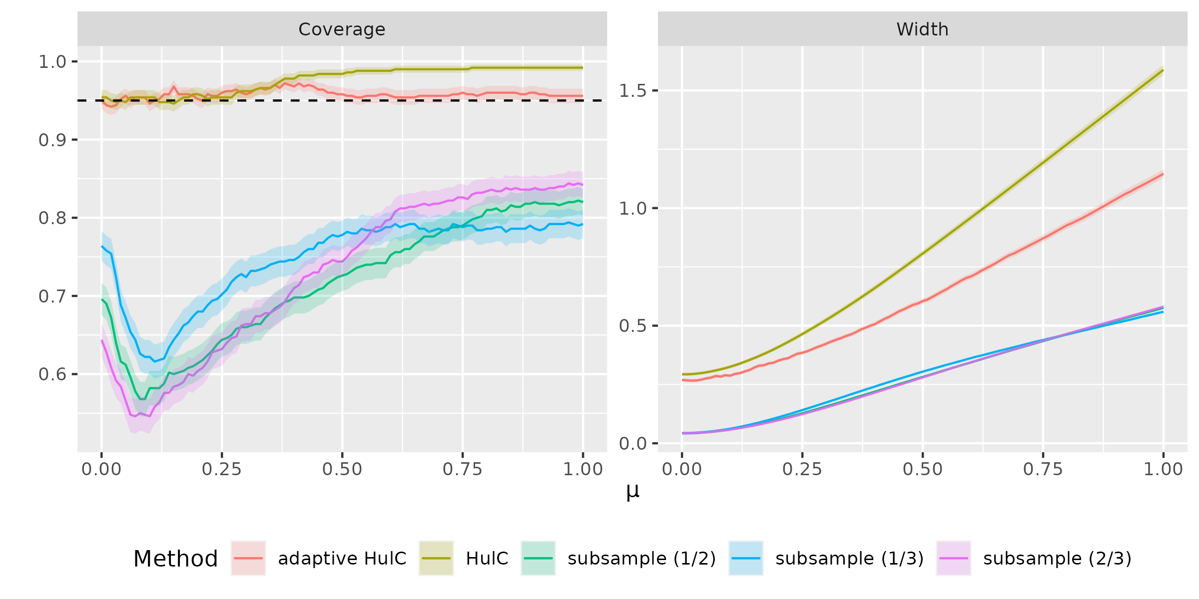
With 100 observations from and varying , Figure 5 shows the performance of several confidence intervals for as changes from to . Note that in this problem, subsampling is not readily applicable because the rate of convergence is unknown (as it depends on ). We use subsampling with estimated rate of convergence from Bertail et al., 1999.
3.6 Uniform model
Suppose are independent real-valued random variables from , the uniform distribution on . The maximum likelihood estimator of from the -th batch is given by which is both mean and median biased. The median bias is and hence Algorithm 1 would be inapplicable because it requires infinitely many splits of the data. Note that in this model, converges to at an rate.
Interestingly, there are estimators of that are median unbiased in this case. For instance, with and representing the largest and the second largest values in , it can be shown that the estimator is finite sample median unbiased for ; see Section 3 of Robson and Whitlock, 1964 for a proof. Hence, Algorithm 1 can be applied with and to obtain a finite-sample valid confidence set for . Note that also has an rate of convergence. In this case, it is known that the classical bootstrap is invalid, but subsampling works; see e.g., Politis and Romano, 1994 and Loh, 1984.
The estimator described above is approximately median unbiased for a large class of distributions of the form for ; see Robson and Whitlock, 1964. Here is an arbitrary distribution function on . Also, see Hall, 1982 for other estimators of , in a large class of non-parametric distributions, that have a limiting distribution that is symmetric around .
3.7 Constrained Estimation
Suppose are independent real-valued random variables with mean . Consider the estimation of . We have seen in Section 3.1 how to apply the HulC for . Although is a simple transformation, it changes the behavior of many commonly used estimators of . This is because is a non-regular functional and hence, there does not exist any regular estimator for ; this follows from Hirano and Porter, 2012. The implication is that classical Wald confidence intervals based on the estimator can fail to cover for close to zero (Robins, 2004, Appendix 1.1). Further, bootstrap and subsampling are also similarly inconsistent; see Fang and Santos, 2019 and Andrews, 2000 for bootstrap, and Andrews and Guggenberger, 2010 for subsampling. It is, however, easy to show that the estimator is asymptotically median unbiased for because is asymptotically median unbiased for . This follows simply from the fact that is monotonic in and hence,
| (34) |
Note that is not strictly increasing. This implies that
| (35) |
Hence, the HulC with the estimator and yields a second-order accurate confidence interval for .
Inequalities (34) and (35) do not require the specific form of the function . They hold for any monotone function and, in particular, for any piecewise constant function. Theorem 3.2 of Fang and Santos, 2019 implies that bootstrap is inconsistent unless is differentiable. This shows the wide range of applicability of our confidence interval. Finally, we note that projection to any set on the real line is a monotone function and hence our confidence interval from the HulC is asymptotically valid with the natural estimator that projects the MLE (or any other estimator) to the constraint set. A simple example where this is useful is in the squared mean estimation example of Section 3.5. The estimator in (31) is not necessarily non-negative, but its target is always non-negative. Using the facts discussed here, we can safely use instead of in the squared mean estimation example.
3.8 Matching Estimators
In causal inference, matching estimators for the average treatment effect (ATE) are popular, partly because they are intuitive. Under certain regularity conditions, matching estimators are known to be asymptotically normal centered at the true ATE. Hence, the HulC with yields a second order accurate confidence interval for ATE. Abadie and Imbens, 2008 proved that the bootstrap is inconsistent for matching estimators. They also commented that subsampling can still be used, but given the computational cost of matching, subsampling becomes computationally intensive with larger samples.
3.9 Semiparametric Estimation
In all the examples above, we have cases where the bootstrap and subsampling are either not easily applicable or fail to provide an asymptotically valid confidence interval. There are many cases where all the usual methods apply but the HulC is much simpler and computationally cheaper.
In non- and semi-parametric problems, when a functional of interest can be estimated by an estimator that is asymptotically normal, two possibilities arise. In the simpler case, the estimator is regular and asymptotically linear with a known (or easily estimable) influence function, while in general the estimator may not have a simple asymptotic expansion. In the first case, we may estimate the asymptotic variance consistently via the sample variance of the (estimated) influence function but obtaining finite-sample guarantees (say via a Berry-Esseen bound) typically requires a case-by-case analysis. More generally however, the variance often involves more nuisance (non-parametric) components than the functional and hence, variance estimation often requires more assumptions or regularity conditions than estimation of the functional. On the other hand, the HulC requires no more nuisance estimation than required for the estimation of the functional. We give three simple examples to illustrate this.
- 1.
Integral functionals of density. Consider the estimation of when are independent and identically distributed observations with a common marginal density supported on a compact set. Theorem 2 of Laurent, 1997 provides an asymptotically efficient estimator for that is asymptotically normal under certain smoothness assumptions on . The asymptotic variance of , however, involves higher order derivatives of when . For a more concrete example, consider the Fisher information functional defined as . The asymptotic variance of the efficient estimator is given by , which involves the second derivative of .
- 2.
Single Index Model. Suppose are independent observations satisfying when is an unknown convex function. Consider the least squares estimator which is obtained as a minimizer of over that is convex, Lipschitz, and in . Kuchibhotla et al., 2021 prove that is asymptotically normal with an asymptotic variance depending on nuisance components such as the conditional mean of on , the derivative of , and the conditional variance of given .
- 3.
Functionals of Normal Models. Suppose are independent observations from in the space (either a Hilbert or a Banach space). Consider the estimation of , if is Banach or , if is Hilbert. Koltchinskii and Zhilova, 2021b; Koltchinskii and Zhilova, 2021a provide asymptotically efficient estimators of which have a normal limiting distribution. Also, see Koltchinskii, 2020. The asymptotic variance is if and is if . Estimating the asymptotic variance hence requires estimating more complicated functionals of . Such variance estimation is not discussed in these works.
In all of these cases our approach using the HulC yields a conceptually simpler confidence interval without any additional nuisance estimation.
4 Adaptive HulC
In this section, we provide a method, the Adaptive HulC, to estimate based on subsampling (Politis and Romano, 1994) and consequently, provide a simple method for constructing a valid confidence interval. One might wonder at this point “why not just use subsampling to construct the confidence interval directly?” The answer is that the Adaptive HulC does not require the knowledge of the rate of convergence of the estimator. As an example, in the mean estimation case with fewer than two finite moments, we do not know the rate of convergence a priori. Further, we do not need to estimate the rate of convergence as suggested in Bertail et al., 1999 for subsampling.
We return now to the univariate parameter setting. Suppose converges in distribution to a continuous random variables as , for some sequence diverging to . Then it follows that
Hence, is the asymptotic median bias and can be estimated using subsampling. Let denote random subsamples of size and let be the estimates based on the subsamples. Let be the estimate based on the full data (of size ). Then can be estimated by
| (36) |
Given this estimator , we can estimate the upper bound on the miscoverage probability in (3) of the convex hull of estimators by . The results of Politis and Romano, 1994 imply that is (asymptotically) consistent for (see also, our Lemma 2, which develops finite-sample bounds) and hence, for large enough ; see Proposition 1. Therefore, the convex hull based on estimators has an asymptotic miscoverage probability of at most . To avoid conservativeness, one can randomize the number of estimators between and to attain asymptotically exact coverage as shown in Algorithm 2. In other words, the output of Algorithm 1 with is the Adaptive HulC interval denoted by
We now prove bounds on the miscoverage probabilities of the confidence intervals of the Adaptive HulC. The first result provides a bound without using the fact that is obtained from subsampling and then using distributional convergence assumptions, we obtain the final miscoverage bound for . Define as the median bias of with , i.e.,
Note that in general depends also on and the true distribution of the data.
Consider the following assumption:
- (A1)
There exists a random variable , a non-decreasing sequence , and a non-increasing sequence converging to zero such that the estimator obtained by applying on observations satisfies
Further, .
Define the asymptotic median bias of the estimation procedure as For any and , define
and for ,
These quantities are taken from Proposition 1 and (11) which implies that for any , if , then . Finally, recall that represents the confidence interval returned by the HulC when the median bias parameter is chosen to be (irrespective of what the true finite sample median bias is).
To succinctly state our next result we define some additional quantities. Given an estimate we compute the number of splits, . We then hypothesize splitting the data twice into and parts with approximately equal number of observations in each split. We then define,
Here are estimators computed based on . We have the following result:
Theorem 3.
Suppose the random variables are independent and assumption (A1) holds true. Then for any , the Adaptive HulC confidence intervals satisfy
| (37) |
and for any ,
| (38) |
Theorem 3 (proved in Section S.8) provides a bound on miscoverage of the confidence interval from Algorithm 2 but does not assume that is obtained from subsampling. The miscoverage probabilities of confidence intervals obtained from non-random choices of number of splits and only requires controlling the probability of . From Proposition 1, it follows that we do not need to be consistent for . Note that the second term in (37) only depends on how close to is.
For the miscoverage probability of that randomizes the number of splits to avoid overcoverage, we require consistency of to . If is obtained from an independent sample, then we would not require such consistency and can apply Theorem 2 to prove miscoverage. Regarding inequality (38), we recall from Theorem 2 (and Remark 2.2) that can be upper and lower bounded by quantities close to . Such lower bounds do not hold true for and . Finally, because is a random selection of one of and , we get
and inequality (37) can be used to imply that has an approximate miscoverage probability of when holds with high probability.
In the multivariate case, one can apply union bound directly on (37) with replaced by to obtain a bound on miscoverage. But using the proof, one can refine this by replacing by . Here is the limiting median bias of the estimator of -th coordinate of and is its estimator. Because the second term on the right hand side of (37) is multiplicative in , a union bound can be safely applied to obtain a non-trivial guarantee, as in Section 7. Similarly, one can replace the first term on the right hand side of (38) with . The second term being multiplicative in does not affect the applicability of a union bound to obtain a non-trivial bound.
Inequality (38) holds true for all . With a consistent estimator for , one can take converging to zero with sample size. In the following, we will prove a bound on when is obtained using subsampling (as in Algorithm 2). It is worth emphasizing that any method of estimating can be used in Theorem 3.
- (A2)
There exists and such that the distribution function of satisfies
- (A3)
The subsample size satisfies and as . Further, the number of subsamples diverges: .
These assumptions are similar to those used in the analysis of subsampling. In contrast to the classical analysis of subsampling by Politis and Romano, 1994 we provide a finite sample analysis.
Lemma 2.
The proof follows a similar structure to that of Politis and Romano, 1994 and appears in Section S.9.
5 Applications to non-standard problems
Many commonly used estimators are derived from classical parametric and semi-parametric efficiency theory and after proper normalization have an asymptotic normal distribution with zero mean. This implies that these estimators have an asymptotic median bias of zero, making them standard problems and allowing for the application of the HulC with . There do exist estimators that have a non-standard rate of convergence and a non-standard limiting distribution. In this section, we discuss four non-standard examples where either the rate of convergence or the limiting distribution or both are unknown in practice. With the rate of convergence unknown, subsampling does not readily apply to yield a confidence interval; one needs to estimate the rate of convergence as in Bertail et al., 1999.
5.1 Squared mean estimation (revisited)
In Section 3.5, we discussed the application of HulC in the context of squared mean estimation. In this application, the rate of convergence of the estimator can be or depending on and as as at different rates, other rates of convergence are possible. Figure 5 shows the performance of HulC (with a conservative median bias bound) and Adaptive HulC and compares them to subsampling. As expected, HulC yields a conservative confidence interval with coverage at least . Subsampling with estimated rate of convergence as in Bertail et al., 1999 fails to attain correct coverage. This can be due to two reasons. First, we fixed the sample size at 100, which might not be large enough for asymptotics of subsampling. Second, subsampling is not uniformly valid in this example. This means that for each (fixed as changes), the coverage asymptotically is at least but if is also allowed to change with the sample size, then subsampling asymptotics break down as shown in Andrews and Guggenberger, 2010. In Figure 5, this can be seen via the dip in the coverage for close enough to ( in our setting). It is very interesting and rather surprising to observe that Adaptive HulC maintains coverage for all and is further close to the nominal for close to and farther away from zero. Although subsampling is not valid for construction of confidence intervals, the estimate of median bias from subsampling, from our experiments, seems to be at least as high as the true median bias.
5.2 Heavy-tailed mean estimation
In Section 3.1, we discussed the application of the HulC in the context of mean estimation when the limiting distribution is symmetric around zero. When the random variables do not have a finite second moment, then the limiting distribution of the sample mean can fail to be symmetric around the population mean with the amount of asymmetry depending on the tail decay on either side of . In this case, the rate of convergence also depends on tail decay and is unknown a priori, which makes subsampling inapplicable. See Romano and Wolf, 1999 for an application of subsampling using the studentized statistic, which does not require estimating the rate of convergence. Without knowing the rate of convergence, we can apply Algorithm 2 to obtain an estimate of the median bias and create a confidence interval for the population mean. In this case, provided that the median bias is not too close to the Adaptive HulC will yield non-trivial confidence intervals.
5.3 Shape constrained regression
Constructing confidence intervals in the context of general non-parametric regression is a difficult task. In order to obtain optimal estimation rates we aim to explicitly balance (squared) bias and variance. On the other hand, the exact bias is often intractable and difficult to account for in confidence interval construction. As a consequence, often under-smoothing is used to ensure that the squared bias is negligible compared to the variance asymptotically. In practice, however, under-smoothing can be sensitive to the precise choice of tuning parameters.
If the conditional mean function is assumed to satisfy a shape constraint such as monotonicity or convexity, then the least squares estimator of the conditional mean has negligible bias uncomplicating the inference problem. However, the rate of convergence and the limiting distribution depends on the local smoothness of the conditional mean. To be concrete, consider the setting of univariate monotone regression with equi-spaced design, i.e., where s are independent and identically distributed with mean zero and finite variance , and is our shape constrained target. Consider the least squares estimator (LSE) of as
Note that is defined uniquely only at , and is, conventionally, defined to as a piecewise constant increasing function on . In this setting, for any such that has a positive continuous derivative on some neighborhood of , the LSE satisfies where has Chernoff’s distribution (here is a two-sided Brownian motion starting from ). It is important here that . If for and (for ), where denotes the -th derivative, then converges to a non-degenerate distribution depending on and . Finally, if is flat at , then the rate of convergence becomes . These results are known in both the fixed and random design settings (see for instance, Wright, 1981; Durot, 2008; Guntuboyina and Sen, 2018). These rates of convergences imply that the LSE admits an adaptive behavior and for arbitrary monotone functions and consequently it is unclear how to perform inference. The situation becomes more complicated in the multi-dimensional case where the limiting distribution depends on the anisotropic smoothness of . Recently Deng et al., 2021 proved that the rates of convergence along with the nuisance parameters in the limiting distributions can be estimated consistently using . This theory requires substantial new techniques and still requires estimation of . Alternatively, we can use the Adaptive HulC in all of these cases to obtain asymptotically valid confidence intervals. It is worth mentioning that in most of these settings, the median bias of the limiting distribution is also unknown because it depends on the unknown local smoothness. The same discussion also holds true for other shape constrained models such as convex regression and current status regression; see Guntuboyina and Sen, 2018 and Deng et al., 2022 for details.
We note that for shape constrained regression, it is possible to obtain confidence bands from confidence intervals at several points on the domain. For example if we know and for two points in the domain, then using the information that is non-decreasing we can conclude that for all , where
| (39) |
Of course, the more points at which confidence intervals are available, the better the confidence band is. Figure 6 shows the simultaneous confidence intervals obtained from the Adaptive HulC (with subsample size and ) for a monotone conditional mean from observations where and . The choice can be obtained by minimizing the bound in Lemma 2 with , which with or represents the rate of convergence of the monotone LSE; see Han and Kato, 2022. This figure only shows one replication of the experiment and suggests that the width of the band seems to adapt to the local smoothness of . In the following subsection, we present one simulation setting for monotone regression comparing the coverage and width of HulC with subsampling. For more simulations comparing the coverage and width of HulC and Adaptive HulC in shape constrained problems, see https://github.com/Arun-Kuchibhotla/HulC/blob/main/R/HulC%20for%20Shape%20Constrained%20Regression.ipynb.
5.3.1 Pointwise Confidence Interval for Monotone Regression
Suppose are independent and identically distributed observations satisfying
Clearly, is a monotonically increasing function on and which implies that is locally -smooth at . From the results of Wright, 1981, it follows that the LSE satisfies converges in distribution to where is the slope at zero of the greatest convex minorant of with being the two-sided Weiner-Levy process with variance one per unit time. Hence, the rate of convergence and the limiting distribution depends curcially on the local smoothness parameter . Experimentally, we verified that is equally likely to be positive or negative and hence, suggests that is asymptotically median unbiased for no matter the value of . With this experimental backing, we applied HulC for this setting and also compared with the performance of subsampling procedure of Bertail et al., 1999 that estimates the rate of convergence with different choices of subsample sizes. Figure 7 shows the comparison of the coverage and width as the sample size changes from 50 to 1000, based on 200 Monte Carlo replications for each sample size and each .

5.4 Nonparametric Regression and Forests
The HulC also yields confidence intervals for nonparametric regression even in the presence of unknown asymptotic mean bias. We briefly sketch the main ideas, deferring most of the details to future work. We focus on constructing a confidence interval for the non-parametric regression function at a fixed point . For example, let be a kernel regression estimator with bandwidth . If is chosen to balance bias and variance then converges to a Gaussian law with mean (which is the asymptotic mean bias), and finite, non-zero variance. As we discussed earlier, classical methods often rely on undersmoothing to ensure that . However, the Adaptive HulC works as long as is finite, since in this case the asymptotic median bias is bounded away from . We also emphasize that, in contrast to undersmoothing for which there are relatively few guidelines on practical implementation, it is more conventional in non-parametric regression to balance (squared) bias and variance, and in many cases cross-validation methods yield tuning parameters which achieve this balancing under various conditions (see for instance, Theorem 2.2 in Li and Racine, 2004).
The argument above is not specific to kernel regression estimators. More generally, let be a complicated nonparametric estimator such as a random forest. The Adaptive HulC yields a valid interval for provided that we are able to balance (squared) bias and variance, i.e. so long as we can ensure that for some possibly unknown , we have that converges to a Gaussian law with possibly non-zero (but finite) mean, and non-zero, finite variance.
6 Confidence Regions under Unimodality
In previous sections, we have considered the construction of confidence intervals based on the median bias of the estimation procedure. In some cases, the estimation procedure has a large median bias close to . For example in the mean square estimation problem, has a median bias of when and in the uniform model, the MLE has a median bias of . In these cases, the HulC and Adaptive HulC are not useful because they would require infinite splits of the data. Interestingly, in these examples, the limiting distribution of the estimation procedure is unimodal at the true parameter. In the univariate setting, unimodality of an estimator at means that the distribution function of the estimator is convex on and concave on . It is important to note that unimodality of a random variable is a global property of the distribution function unlike median bias, which is a local property.
Using the results of Lanke, 1974, we can construct a confidence interval based on unimodality of the estimation procedure. The resulting confidence interval is very similar to the one from the HulC. The Unimodal HulC method is presented in Algorithm 3.
| (40) |
The Unimodal HulC can be seen as a generalization of the HulC where we also use the unimodality of estimators, if available. Unimodal HulC involves a tuning parameter indicates how much to inflate the convex hull confidence interval. Taking in the Unimodal HulC gives exactly the HulC. The confidence interval with need not have coverage validity if the asymptotic median bias is and by taking , we get asymptotic coverage when the limiting distribution is unimodal even if the asymptotic median bias is . Even if , using yields a reduction in the number of estimators used for convex hull. Formally, set , which is upper bounded by . Then Unimodal HulC only requires many independent estimators, where is the smallest integer such that .
In the Unimodal HulC, we assume that the limiting median bias is known, but one can always substitute if median bias is unknown; recall that for all . Instead of assuming a known , one can use the subsampling approach from Section 4 to replace with the subsampling estimator. We leave it to future work to derive a final miscoverage bound for this subsampling-based procedure.
The following theorem (proved in Section S.10) shows that the confidence interval returned by the Unimodal HulC has a miscoverage probability bounded asymptotically by .
Theorem 4.
Suppose the estimators in the Unimodal HulC are independent and are constructed based on approximately equal sized samples. Further, suppose the estimators are continuously distributed and satisfy
| (41) |
for some sequence and a continuous random variable that is unimodal at and has a median bias of (i.e., ). Then for all , , and ,
| (42) |
Similar to Theorem 2, Theorem 4 shows that the confidence interval from the Unimodal HulC has its miscoverage probability bounded by up to a multiplicative error. Once again, this is unlike the coverage guarantee for Wald’s interval. Because of the multiplicative error, the guarantee from Theorem 4 is also suitable for an application of the union bound to obtain a valid multivariate confidence region, as discussed previously in Section 7.
Note that the right hand side of (42) is finite if and only if . It is easy to prove that when either or and in many cases, . Hence, the condition for finiteness would hold true as long as ; this is similar to the requirement in the HulC. The importance of the Unimodal HulC stems from its ability to tackle problems where the median bias of the estimator is large (near ).
The width of the confidence interval is given by . This is times larger than the width of confidence interval from the HulC. The confidence interval has asymptotically valid coverage of at least for any parameter and as increases, the number of splits in the Unimodal HulC decreases leading to a smaller value of . Similar to the map , the map is a piecewise constant function.
6.1 Standard problems (revisited)
The Unimodal HulC can make use of both asymptotic unimodality and asymptotic median unbiasedness which holds true for most of the standard problems where the limiting distribution is Gaussian (a symmetric unimodal distribution). In many of the examples discussed in Section 3, one can use the Unimodal HulC to (potentially) obtain a tighter confidence interval. Note that in the Unimodal HulC is always smaller than in the HulC. Once again the advantage is that we do not need to estimate the limiting variance of the estimators being used and need not know the rate of convergence.
6.2 Application 2: shape constrained regression (revisited)
In Section 5.3, we used subsampling to estimate the median bias of the LSE in shape constrained regression. Experimentally, we found that the distribution of the LSE is unimodal at the true value. Consider the regression problem where and . The histograms of the LSE error for ranging from to are shown in Figure 8 when the estimator is computed based on samples and 1000 replications. Figure 8 indicates that the distribution of has a unique mode and that mode is close to zero, and this property is unaffected by the location of .
We are not aware of a result proving unimodality of the limiting distribution of the LSE in general (when higher derivatives of may vanish at ). But, motivated by our experimental results, we apply the Unimodal HulC to construct a confidence band, and leave a more rigorous investigation of its validity to future work.
The performance of the Unimodal HulC for monotone regression is shown in Figure 9; for illustration, we use . It shows adaptation and shows higher uncertainty around the change point. The confidence band here is noticeably larger than the one from the Adaptive HulC.
7 HulC for multivariate parameters
Suppose now that . A slight modification of the HulC still works if we replace the interval with either the convex hull or the rectangular hull of the estimators.
As before, let be independent estimators of . The convex hull of a set of points in is the smallest convex set containing these points. The smallest rectangle containing the estimators , which we call the rectangular hull, is
where represent the canonical basis vectors in ; and denotes the Cartesian product.
To compactly state our next result, we define the following coordinate-wise maximum median bias,
| (43) |
Similar to Lemma 1, we have the following result (proved in Section S.6) on the coverage of the convex hull and the smallest rectangle.
Lemma 3.
Suppose are independent estimators of .
- 1.
If for all , then for ,
(44) - 2.
Recall the definition of in (43). For all ,
(45)
The proof of (44) follows from the works of Wendel, 1962 and Wagner and Welzl, 2001. The requirement of more than estimators can be restrictive in practice. This is especially so in near high dimensional problems where the dimension can grow with the sample size . The proof of (45) follows by using the union bound on the univariate confidence region in Lemma 1. Furthermore, to obtain (45) we only assume that the coordinate-wise median bias of the estimators is bounded and this condition is much weaker than the corresponding condition used to obtain (44).
Inequality (45) is written with a single parameter as a bound on the median bias for all coordinates. It is, however, easy to obtain similar bounds when the median bias is different for different coordinates; see the proof of Lemma 3 for details. Similarly, we also note that, one need not compute random vector estimators. One might construct a different number of estimators for and construct univariate confidence intervals along each coordinate to obtain a multivariate confidence rectangle for . Formally, if is a confidence interval of level for constructed using Algorithm 1 with (a known) , then
| (46) |
Note that construction of requires estimators of . Following inequalities (8), we conclude that
This implies that one only needs to split the original data into (about) many batches. In Lemma 3, (45) requires for a constant for a coverage of . This can be compared with the requirement for the validity of (44). Hence, for moderate to high dimensional problems, the smallest rectangle is an economical choice.
Similar to the univariate case, one need not know median bias of exactly. It suffices to know it approximately as dictated by Proposition 1. The conclusions from Proposition 1 continue to hold true even with a growing dimension. For instance, for asymptotically median unbiased estimators, if
| (47) |
for some constant , then irrespective of the dimension , we obtain
It follows from Figures S.1 & S.2 that the right hand side of (47) can be as large as for certain choices of , even for . Similarly, Theorem 2 (in particular its implication (19)) yields
| (48) |
Here the union bound is valid irrespective of what the dimension is relative to the sample size . If the estimators are median bias reduced, then the same argument as above yields
| (49) |
Note, once again, that and hence the miscoverage probabilities are bounded by (under (14)) and (under median bias reduction).
We see that we only require (or in the bias reduced case) and we do not require joint/multivariate distributional convergence whatsoever. This can be contrasted with the results from the literature on high-dimensional central limit theorems (Belloni et al., 2018; Koike, 2021; Fang and Koike, 2021; Deng, 2020; Chernozhukov et al., 2020). These results concern Gaussian approximation for high-dimensional averages. Under certain moment assumptions on the joint distribution, these results imply a joint Gaussian approximation with a minimum requirement of (Fang and Koike, 2021, Proposition 1.1). Belloni et al., 2018 uses the union bound based on moderate deviations but still requires joint moment conditions and the condition that . With usual estimators, the HulC also has the same dimensionality requirement while only making use of marginal median bias. With median bias reduced estimators, the HulC only requires and this is even weaker than , which is the best possible dimension restriction for a Gaussian approximation (Das and Lahiri, 2021, Theorem 3). It is worth mentioning that by slightly enlarging the bootstrap confidence regions, the dimensionality requirement can be reduced to in the case of mean estimation (Deng, 2020).
Although we have used the union bound above to obtain a coverage of for a multivariate parameter, we only required asymptotic median unbiasedness of marginally. There is no requirement whatsoever on the asymptotic joint convergence or symmetry of . Interestingly, such a result is not possible with the usual confidence intervals. This point is discussed further in Section S.1 of the supplementary material.
8 Conclusions and Future Directions
In this paper, we developed and analyzed a simple and broadly applicable method, the HulC , for constructing confidence sets, using the convex hull of estimates constructed on independent subsamples of the data. All the HulC intervals presented have an asymptotic coverage either equal to or greater than . The HulC bypasses the difficult problem of estimating nuisance components in the limiting distribution, requires fewer regularity conditions than the bootstrap and unlike subsampling does not require knowledge of the rate of convergence of the underlying estimates on which it is based. These advantages, in many cases, come at a surprisingly small price in the width of the interval. The width of the intervals are determined in general by the accuracy of the underlying estimators, as well as their median bias. We also present two variants, the Adaptive HulC which estimates the median bias using subsampling, and the Unimodal HulC which can be useful even in cases when the median bias is large so long as the limiting distribution is unimodal. Beyond these methodological contributions, we also studied several challenging confidence set construction problems and showed how our methods can often provide simple solutions to these problems.
From a computational standpoint, the HulC only requires computing the estimator times where is typically around 5 or 10, and so is less computationally intensive than the bootstrap. In cases where the underlying estimator has computational complexity which is super-linear in the number of samples, computing estimates on samples can in fact be cheaper than computing a single estimate on the whole dataset. These considerations are relevant no matter the dimension of the estimator.
Intuitively, the HulC is also quite robust in the sense that we only use qualitative properties, such as an upper bound on the median bias, of the limiting distribution rather than its exact form. In finite samples, the distribution of a statistic might be close to symmetric even if it does not resemble a Gaussian distribution.
Our analysis has not discussed the important problem of obtaining confidence intervals with uniform coverage. This is especially important in irregular problems where the rate of convergence and limiting distribution can vary across the parameter space. Developing this understanding is an important open problem that we plan to address in future work.
Acknowledgements
We are grateful to Prof. Hannes Leeb for helpful comments, and for pointing out a gap in an earlier version of Theorem 1 and Proposition 1. We also thank Jin-Hong Du for his help with Figures 2–5. We also thank the reviewers and the associate editor for their constructive comments that led to several improvements of the paper.
References
- Abadie and Imbens, (2008) Abadie, A. and Imbens, G. W. (2008). On the failure of the bootstrap for matching estimators. Econometrica, 76(6):1537–1557.
- Andrews, (2000) Andrews, D. W. K. (2000). Inconsistency of the bootstrap when a parameter is on the boundary of the parameter space. Econometrica, 68(2):399–405.
- Andrews and Guggenberger, (2010) Andrews, D. W. K. and Guggenberger, P. (2010). Asymptotic size and a problem with subsampling and with the out of bootstrap. Econometric Theory, 26(2):426–468.
- Andrews and Phillips, (1987) Andrews, D. W. K. and Phillips, P. C. B. (1987). Best median-unbiased estimation in linear regression with bounded asymmetric loss functions. J. Amer. Statist. Assoc., 82(399):886–893.
- Athreya, (1987) Athreya, K. B. (1987). Bootstrap of the mean in the infinite variance case. Ann. Statist., 15(2):724–731.
- Belloni et al., (2018) Belloni, A., Chernozhukov, V., Chetverikov, D., Hansen, C., and Kato, K. (2018). High-dimensional econometrics and regularized GMM. arXiv preprint arXiv:1806.01888.
- Bentkus, (2005) Bentkus, V. (2005). A Lyapunov type bound in . Theory Probab. Appl., 49(2):311–323.
- Bentkus et al., (1997) Bentkus, V., Bloznelis, M., and Götze, F. (1997). A Berry-Esséen bound for -estimators. Scand. J. Statist., 24(4):485–502.
- Bertail and Politis, (2001) Bertail, P. and Politis, D. N. (2001). Extrapolation of subsampling distribution estimators: the i.i.d. and strong mixing cases. Canad. J. Statist., 29(4):667–680.
- Bertail et al., (1999) Bertail, P., Politis, D. N., and Romano, J. P. (1999). On subsampling estimators with unknown rate of convergence. J. Amer. Statist. Assoc., 94(446):569–579.
- Bickel, (1982) Bickel, P. J. (1982). On adaptive estimation. Ann. Statist., 10(3):647–671.
- Bickel et al., (1993) Bickel, P. J., Klaassen, C. A. J., Ritov, Y., and Wellner, J. A. (1993). Efficient and adaptive estimation for semiparametric models. Johns Hopkins Series in the Mathematical Sciences. Johns Hopkins University Press, Baltimore, MD.
- Birnbaum, (1964) Birnbaum, A. (1964). Median-unbiased estimators. Bull. Math. Statist., 11(1-2):25–34.
- Borges, (6970) Borges, R. (1969/70). Eine Approximation der Binomialverteilung durch die Normalverteilung der Ordnung . Z. Wahrscheinlichkeitstheorie und Verw. Gebiete, 14:189–199.
- Borges, (1971) Borges, R. (1971). Derivation of normalizing transformations with an error of order . Sankhyā Ser. A, 33:441–460.
- Boucheron and Thomas, (2012) Boucheron, S. and Thomas, M. (2012). Concentration inequalities for order statistics. Electron. Commun. Probab., 17:no. 51, 12.
- Breiman, (1992) Breiman, L. (1992). Probability, volume 7 of Classics in Applied Mathematics. Society for Industrial and Applied Mathematics (SIAM), Philadelphia, PA. Corrected reprint of the 1968 original.
- Brown et al., (2001) Brown, L. D., Cai, T. T., and DasGupta, A. (2001). Interval estimation for a binomial proportion. Statist. Sci., 16(2):101–133. With comments and a rejoinder by the authors.
- Brown et al., (2002) Brown, L. D., Cai, T. T., and DasGupta, A. (2002). Confidence intervals for a binomial proportion and asymptotic expansions. Ann. Statist., 30(1):160–201.
- Brown et al., (1976) Brown, L. D., Cohen, A., and Strawderman, W. E. (1976). A complete class theorem for strict monotone likelihood ratio with applications. Ann. Statist., 4(4):712–722.
- Buja et al., (2019) Buja, A., Brown, L., Berk, R., George, E., Pitkin, E., Traskin, M., Zhang, K., and Zhao, L. (2019). Models as approximations I: consequences illustrated with linear regression. Statist. Sci., 34(4):523–544.
- Cabrera and Watson, (1997) Cabrera, J. and Watson, G. (1997). Simulation methods for mean and median bias reduction in parametric estimation. Journal of statistical planning and inference, 57(1):143–152.
- Chakravarti et al., (2019) Chakravarti, P., Balakrishnan, S., and Wasserman, L. (2019). Gaussian mixture clustering using relative tests of fit. arXiv preprint arXiv:1910.02566.
- Chernozhukov et al., (2020) Chernozhukov, V., Chetverikov, D., and Koike, Y. (2020). Nearly optimal central limit theorem and bootstrap approximations in high dimensions. arXiv preprint arXiv:2012.09513.
- Das and Lahiri, (2021) Das, D. and Lahiri, S. (2021). Central Limit Theorem in high dimensions: the optimal bound on dimension growth rate. Trans. Amer. Math. Soc., 374(10):6991–7009.
- Deng, (2020) Deng, H. (2020). Slightly conservative bootstrap for maxima of sums. arXiv preprint arXiv:2007.15877.
- Deng et al., (2022) Deng, H., Han, Q., and Sen, B. (2022). Inference for local parameters in convexity constrained models. Journal of the American Statistical Association, (just-accepted):1–33.
- Deng et al., (2021) Deng, H., Han, Q., and Zhang, C.-H. (2021). Confidence intervals for multiple isotonic regression and other monotone models. Ann. Statist., 49(4):2021–2052.
- Desu and Rodine, (1969) Desu, M. M. and Rodine, R. H. (1969). Estimation of the population median. Scandinavian Actuarial Journal, 1969(1-2):67–70.
- Doerr, (2018) Doerr, B. (2018). An elementary analysis of the probability that a binomial random variable exceeds its expectation. Statist. Probab. Lett., 139:67–74.
- Dümbgen, (1993) Dümbgen, L. (1993). On nondifferentiable functions and the bootstrap. Probab. Theory Related Fields, 95(1):125–140.
- Durot, (2008) Durot, C. (2008). Monotone nonparametric regression with random design. Math. Methods Statist., 17(4):327–341.
- Efron, (1979) Efron, B. (1979). Bootstrap methods: another look at the jackknife. Ann. Statist., 7(1):1–26.
- Efron, (1982) Efron, B. (1982). Transformation theory: how normal is a family of distributions? Ann. Statist., 10(2):323–339.
- Fang and Koike, (2021) Fang, X. and Koike, Y. (2021). High-dimensional central limit theorems by Stein’s method. Ann. Appl. Probab., 31(4):1660–1686.
- Fang and Santos, (2019) Fang, Z. and Santos, A. (2019). Inference on directionally differentiable functions. Rev. Econ. Stud., 86(1):377–412.
- Firth, (1993) Firth, D. (1993). Bias reduction of maximum likelihood estimates. Biometrika, 80(1):27–38.
- Gebhardt, (1969) Gebhardt, F. (1969). Some numerical comparisons of several approximations to the binomial distribution. J. Amer. Statist. Assoc., 64(328):1638–1646.
- Greenberg and Mohri, (2014) Greenberg, S. and Mohri, M. (2014). Tight lower bound on the probability of a binomial exceeding its expectation. Statist. Probab. Lett., 86:91–98.
- Guntuboyina and Sen, (2018) Guntuboyina, A. and Sen, B. (2018). Nonparametric shape-restricted regression. Statist. Sci., 33(4):568–594.
- Hall, (1982) Hall, P. (1982). On estimating the endpoint of a distribution. Ann. Statist., 10(2):556–568.
- Hall, (1986) Hall, P. (1986). On the bootstrap and confidence intervals. Ann. Statist., 14(4):1431–1452.
- Hall, (1988) Hall, P. (1988). Theoretical comparison of bootstrap confidence intervals. Ann. Statist., 16(3):927–985. With a discussion and a reply by the author.
- Hall, (1992) Hall, P. (1992). The bootstrap and Edgeworth expansion. Springer Series in Statistics. Springer-Verlag, New York.
- Hamza, (1995) Hamza, K. (1995). The smallest uniform upper bound on the distance between the mean and the median of the binomial and Poisson distributions. Statist. Probab. Lett., 23(1):21–25.
- Han and Kato, (2022) Han, Q. and Kato, K. (2022). Berry–Esseen bounds for Chernoff-type nonstandard asymptotics in isotonic regression. Ann. Appl. Probab., 32(2):1459–1498.
- Hartigan, (1969) Hartigan, J. A. (1969). Using subsample values as typical values. J. Amer. Statist. Assoc., 64:1303–1317.
- Hartigan, (1970) Hartigan, J. A. (1970). Exact confidence intervals in regression problems with independent symmetric errors. Ann. Math. Statist., 41:1992–1998.
- Hayakawa et al., (2021) Hayakawa, S., Lyons, T., and Oberhauser, H. (2021). Estimating the probability that a given vector is in the convex hull of a random sample. arXiv preprint arXiv:2101.04250.
- Hirano and Porter, (2012) Hirano, K. and Porter, J. R. (2012). Impossibility results for nondifferentiable functionals. Econometrica, 80(4):1769–1790.
- Hirji et al., (1989) Hirji, K. F., Tsiatis, A. A., and Mehta, C. R. (1989). Median unbiased estimation for binary data. Amer. Statist., 43(1):7–11.
- Hoeffding, (1963) Hoeffding, W. (1963). Probability inequalities for sums of bounded random variables. J. Amer. Statist. Assoc., 58:13–30.
- Ibragimov and Müller, (2010) Ibragimov, R. and Müller, U. K. (2010). -statistic based correlation and heterogeneity robust inference. J. Bus. Econom. Statist., 28(4):453–468.
- Jing et al., (2003) Jing, B.-Y., Shao, Q.-M., and Wang, Q. (2003). Self-normalized Cramér-type large deviations for independent random variables. Ann. Probab., 31(4):2167–2215.
- John, (1974) John, S. (1974). Median-unbiased most acceptable estimates of Poisson, binomial and negative-binomial distributions. Comm. Statist., 3:1155–1159.
- Kabluchko and Zaporozhets, (2019) Kabluchko, Z. and Zaporozhets, D. (2019). Expected volumes of Gaussian polytopes, external angles, and multiple order statistics. Trans. Amer. Math. Soc., 372(3):1709–1733.
- Kenne Pagui et al., (2017) Kenne Pagui, E. C., Salvan, A., and Sartori, N. (2017). Median bias reduction of maximum likelihood estimates. Biometrika, 104(4):923–938.
- Kim, (2016) Kim, K. I. (2016). Higher order bias correcting moment equation for m-estimation and its higher order efficiency. Econometrics, 4(4):48.
- Knight, (1989) Knight, K. (1989). On the bootstrap of the sample mean in the infinite variance case. Ann. Statist., 17(3):1168–1175.
- Knight, (1998) Knight, K. (1998). Limiting distributions for regression estimators under general conditions. Ann. Statist., 26(2):755–770.
- Knight, (1999) Knight, K. (1999). Asymptotics for -estimators of regression parameters under heteroscedasticityy. Canadian Journal of Statistics, 27(3):497–507.
- Knight, (2008) Knight, K. (2008). Asymptotics of the regression quantile basic solution under misspecification. Applications of Mathematics, 53(3):223–234.
- Koike, (2021) Koike, Y. (2021). Notes on the dimension dependence in high-dimensional central limit theorems for hyperrectangles. Jpn. J. Stat. Data Sci., 4(1):257–297.
- Koltchinskii, (2020) Koltchinskii, V. (2020). Estimation of smooth functionals in high-dimensional models: bootstrap chains and gaussian approximation. arXiv preprint arXiv:2011.03789.
- (65) Koltchinskii, V. and Zhilova, M. (2021a). Efficient estimation of smooth functionals in Gaussian shift models. Ann. Inst. Henri Poincaré Probab. Stat., 57(1):351–386.
- (66) Koltchinskii, V. and Zhilova, M. (2021b). Estimation of smooth functionals in normal models: bias reduction and asymptotic efficiency. Ann. Statist., 49(5):2577–2610.
- Kosmidis and Firth, (2009) Kosmidis, I. and Firth, D. (2009). Bias reduction in exponential family nonlinear models. Biometrika, 96(4):793–804.
- Kosmidis et al., (2020) Kosmidis, I., Kenne Pagui, E. C., and Sartori, N. (2020). Mean and median bias reduction in generalized linear models. Stat. Comput., 30(1):43–59.
- Kuchibhotla, (2021) Kuchibhotla, A. K. (2021). Median bias of M-estimators. arXiv preprint arXiv:2106.00164.
- Kuchibhotla et al., (2023) Kuchibhotla, A. K., Balakrishnan, S., and Wasserman, L. (2023). Median regularity and honest inference. Biometrika, Accepted.
- Kuchibhotla et al., (2021) Kuchibhotla, A. K., Patra, R. K., and Sen, B. (2021). Semiparametric efficiency in convexity constrained single index model. J. Amer. Statist. Assoc.
- Lam, (2022) Lam, H. (2022). A cheap bootstrap method for fast inference. arXiv preprint arXiv:2202.00090.
- Lanke, (1974) Lanke, J. (1974). Interval estimation of a median. Scand. J. Statist., 1(1):28–32.
- Laurent, (1997) Laurent, B. (1997). Estimation of integral functionals of a density and its derivatives. Bernoulli, 3(2):181–211.
- Lehmann, (1959) Lehmann, E. L. (1959). Testing statistical hypotheses. John Wiley & Sons, Inc., New York; Chapman & Hall, Ltd., London.
- Lehmann and Casella, (1998) Lehmann, E. L. and Casella, G. (1998). Theory of point estimation. Springer Texts in Statistics. Springer-Verlag, New York, second edition.
- Li and Racine, (2004) Li, Q. and Racine, J. (2004). Cross-validated local linear nonparametric regression. Statist. Sinica, 14(2):485–512.
- Loh, (1984) Loh, W.-Y. (1984). Estimating an endpoint of a distribution with resampling methods. Ann. Statist., 12(4):1543–1550.
- Mammen, (1992) Mammen, E. (1992). Bootstrap, wild bootstrap, and asymptotic normality. Probab. Theory Related Fields, 93(4):439–455.
- Massart, (1990) Massart, P. (1990). The tight constant in the Dvoretzky-Kiefer-Wolfowitz inequality. Ann. Probab., 18(3):1269–1283.
- (81) Pfanzagl, J. (1970a). Median unbiased estimates for M. L. R.-families. Metrika, 15:30–39.
- (82) Pfanzagl, J. (1970b). On the asymptotic efficiency of median unbiased estimates. Ann. Math. Statist., 41:1500–1509.
- Pfanzagl, (1971) Pfanzagl, J. (1971). The Berry-Esseen bound for minimum contrast estimates. Metrika, 17:82–91.
- Pfanzagl, (7172) Pfanzagl, J. (1971/72). On median unbiased estimates. Metrika, 18:154–173.
- (85) Pfanzagl, J. (1973a). Asymptotic expansions related to minimum contrast estimators. Ann. Statist., 1:993–1026.
- (86) Pfanzagl, J. (1973b). Asymptotic expansions related to minimum contrast estimators. The Annals of Statistics, pages 993–1026.
- Pfanzagl, (1979) Pfanzagl, J. (1979). On optimal median unbiased estimators in the presence of nuisance parameters. Ann. Statist., 7(1):187–193.
- Pfanzagl, (1994) Pfanzagl, J. (1994). Parametric statistical theory. De Gruyter Textbook. Walter de Gruyter & Co., Berlin. With the assistance of R. Hamböker.
- Pfanzagl, (2017) Pfanzagl, J. (2017). Optimality of unbiased estimators: Nonasymptotic theory. In Mathematical Statistics, Springer Series in Statistics, pages 83–106. Springer-Verlag, Berlin. Essays on history and methodology, Springer Series in Statistics. Perspectives in Statistics.
- Pinelis, (2017) Pinelis, I. (2017). Optimal-order uniform and nonuniform bounds on the rate of convergence to normality for maximum likelihood estimators. Electron. J. Stat., 11(1):1160–1179.
- Politis and Romano, (1994) Politis, D. N. and Romano, J. P. (1994). Large sample confidence regions based on subsamples under minimal assumptions. Ann. Statist., 22(4):2031–2050.
- Read, (2004) Read, C. B. (2004). Median unbiased estimators. Encyclopedia of statistical sciences, 7.
- Rinaldo et al., (2019) Rinaldo, A., Wasserman, L., and G’Sell, M. (2019). Bootstrapping and sample splitting for high-dimensional, assumption-lean inference. Ann. Statist., 47(6):3438–3469.
- Robins, (2004) Robins, J. M. (2004). Optimal structural nested models for optimal sequential decisions. In Proceedings of the Second Seattle Symposium in Biostatistics, volume 179 of Lect. Notes Stat., pages 189–326. Springer, New York.
- Robson and Whitlock, (1964) Robson, D. S. and Whitlock, J. H. (1964). Estimation of a truncation point. Biometrika, 51:33–39.
- Romano and Wolf, (1999) Romano, J. P. and Wolf, M. (1999). Subsampling inference for the mean in the heavy-tailed case. Metrika, 50(1):55–69.
- Sen, (1968) Sen, P. K. (1968). Asymptotic normality of sample quantiles for -dependent processes. Ann. Math. Statist., 39:1724–1730.
- Shao and Tu, (1995) Shao, J. and Tu, D. S. (1995). The jackknife and bootstrap. Springer Series in Statistics. Springer-Verlag, New York.
- Shao, (1997) Shao, Q.-M. (1997). Self-normalized large deviations. Ann. Probab., 25(1):285–328.
- Sherman and Carlstein, (2004) Sherman, M. and Carlstein, E. (2004). Confidence intervals based on estimators with unknown rates of convergence. Comput. Statist. Data Anal., 46(1):123–139.
- Stigler, (2007) Stigler, S. M. (2007). The epic story of maximum likelihood. Statist. Sci., 22(4):598–620.
- van der Vaart, (1998) van der Vaart, A. W. (1998). Asymptotic statistics, volume 3 of Cambridge Series in Statistical and Probabilistic Mathematics. Cambridge University Press, Cambridge.
- Wagner and Welzl, (2001) Wagner, U. and Welzl, E. (2001). A continuous analogue of the upper bound theorem. volume 26, pages 205–219. ACM Symposium on Computational Geometry (Hong Kong, 2000).
- Wasserman et al., (2020) Wasserman, L., Ramdas, A., and Balakrishnan, S. (2020). Universal inference. Proc. Natl. Acad. Sci. USA, 117(29):16880–16890.
- Wendel, (1962) Wendel, J. G. (1962). A problem in geometric probability. Math. Scand., 11:109–111.
- Wright, (1981) Wright, F. T. (1981). The asymptotic behavior of monotone regression estimates. Ann. Statist., 9(2):443–448.
- Zhang and Liang, (2011) Zhang, J.-J. and Liang, H.-Y. (2011). Berry-Esseen type bounds in heteroscedastic semi-parametric model. J. Statist. Plann. Inference, 141(11):3447–3462.
Supplement to
“The HulC: Confidence Regions from Convex Hulls”
S.1 Union bound with Wald intervals
If, for each , the estimators are asymptotically normal, then asymptotic normality implies that for all ,
for some converging to zero as ; an example is (13). First order accurate confidence intervals (such as Wald’s) satisfy , second order accurate ones satisfy and so on. Taking and applying the union bound, we only obtain
In order for the right hand side to be asymptotically, one needs . This is a very stringent requirement, especially when the dimension grows faster than the sample size .
There is a simple way to resolve this issue following our proposed methodology. The idea is to construct Wald confidence regions for each coordinate from each of and then take the union of these regions. Formally, set . For , suppose is the Wald confidence region of coverage based on . This means that
The right hand side here depends on the dimension because is computed based on many observations. Under these conditions, the following result provides a valid confidence regions using Wald’s confidence intervals and a union bound. The interesting aspect (similar to (12)) is that the coverage implied by Proposition 3 is eventually finite sample (i.e., holds after some sample size) even though the coverage of is asymptotic.
Proposition 3.
If
| (E.1) |
then
Proof.
Similar to the right hand side of (9), the right hand side of (E.1) is be bounded away from zero unless is a power of . It is worth noting that, unlike (12), the construction of the confidence region requires estimation of variance of the estimators and its validity requires (marginal) distributional convergence of the estimators .
S.2 Proof of Lemma 1
S.3 Proof of Theorem 1
The confidence interval from the HulC is either based on estimators or based on estimators. The number of estimators used depends on the realization of the uniform random variable in step 2 of the HulC. With probability , the confidence interval will be based on estimators and with probability , the confidence interval will be based on estimators. Hence from Lemma 1, we obtain
| (E.2) |
This proves (6). Under the additional assumptions for (7), the only inequality in (E.2) becomes equality. Firstly, for all implies that
Secondly, the assumption that all the estimators have a median bias of exactly, implies that this probability is exactly . This proves (7).
S.4 Proof of Proposition 1
If , then the conclusion is obvious. Consider the case, . Note that is an increasing function of . Hence, for any , we have
| (E.3) |
Reversing the roles of and , we conclude that if , then
Hence, for all , and all , we have
| (E.4) |
Because , using (E.4) with , we get if
| (E.5) |
Similarly, , using (E.4) with , we get if
| (E.6) |
Note that both the ratios on the right hand side of (E.5) and (E.6) are at least . Furthermore, inequality (E.6) will be satisfied if Combining inequalities (E.5) and (E.6), we get that if (9) holds true, then and hence .
Note that in inequality (E.3), we used an inequality for the ratio . Observe that if , then has zero derivative at . Observe that, with ,
for some . For , the right most term is zero and for we have that
Because , we obtain for all ,
| (E.7) |
By definition . Taking in (E.7), we obtain
| (E.8) |
Again by definition . Taking in (E.7), we obtain
| (E.9) |

S.5 Proof of Theorem 2
Because the median bias of estimators from is , we set
Lemma 1 implies that
The right hand side involves an expectation because is a random variable satisfying
This follows from (4). Therefore,
| (E.10) |
From the proof of Proposition 1 (in particular (E.7)), it follows that
| (E.11) |
Substituting this inequality in (E.10) yields
The last equality follows from the definition (4) of . This completes the proof of upper bound in (17).
From the proof of Lemma 1, it follows, under the assumption of and the exact median bias of , that
the last equality follows again from the definition of in (4). This completes the proof of (18).
For the case where the estimators have an asymptotic median bias of (), we use the HulC to obtain , while the true finite sample median bias is bounded by . In this case, to prove the upper bound, we use the inequality
in place of (E.11). Using this inequality in (E.10) (with replaced by ), we obtain
From the proof of Lemma 1, it follows, under the assumption of and the exact median bias of , that
This proves the upper and lower bounds for a non-zero asymptotic median bias of .
S.6 Proof of Lemma 3
Equality (44) follows from Theorem 3 of Hayakawa et al., 2021. This result was originally proved in Wendel, 1962 under symmetry of . Wagner and Welzl, 2001 proved that the miscoverage probability is lower bounded by the quantity on the right hand side whenever has an absolutely continuous distribution; this does not require the assumption of for all .
S.7 Proof of Proposition 2
For notational convenience and without loss of generality, we will prove the result when is computed based on observations. Set
This can be rewritten as
In terms of and , this becomes
It is clear that
Set . By the univariate Berry–Esseen bound, we get
| (E.12) |
Similarly,
| (E.13) |
Inequality (E.12) implies that
Clearly,
| (E.14) |
Similarly,
| (E.15) |
Note that
| (E.16) |
Using inequality (E.13), we obtain
Finally, note that
Combining the two inequalities above, we get
| (E.17) |
Substituting these inequalities in (E.14) and (E.15), we conclude
| (E.18) |
Here
This implies
Note that the right hand side of (E.18) is of order and does not depend on ; it only depends on . Inequality (E.18) implies that the median bias of can be obtained by taking the maximum over all of
It seems the maximum is attained at for any .
S.8 Proof of Theorem 3
Throughout the proof, we write instead of for convenience. Define the event
and set
| (E.19) |
Recall from (4). On the event , we get that
We first bound the miscoverage probabilities of and when event occurs. From the definition of and Lemma 1,
| (E.20) |
The first inequality follows from proof of Proposition 1 (in particular (E.4)) while the second inequality follows from the fact that and for any . Similarly,
| (E.21) |
This completes the proof of (37). We will now prove a bound on the miscoverage probability of . Writing to represent the expectation with respect to which is a uniform random variable independent of the data, we get
| (E.22) |
Note that the miscoverage probability of is . Using inequalities (E.20) and (E.21), we can readily obtain
If , this only implies approximately miscoverage probability. If converges to zero in probability, then converges to zero and we obtain asymptotically miscoverage probability for . This is the aim in proving (38). For this, we cannot readily use inequality (37) because depend on the same data as and . In order to overcome this, we show is close to in a relative error sense. For this, it is not sufficient to know . We need to be small. Consider the event
for some . Recall from Proposition 1 implies that if , then . Hence, if , then and . To control the difference between and , we write as
where and . Similarly, we can write for defined similar to with replacing . From inequalities (E.4) and (E.7), we get that
The same inequalities also hold true for . For notational convenience, let us write and the same for . It is easy to verify that is a decreasing function of and and hence
Recall that and . It follows that
This yields
Hence, on event ,
| (E.23) |
Note that is non-random and only depends on in the event . Inequality (E.23) can be alternatively written as .
From (E.22) and the fact that for on the event (when ), we get
| (E.24) |
Because
it follows from (E.24) and (E.23) that
| (E.25) |
The second reminder term in (E.25) is controlled using the definition of in (E.23) and the bounds (E.20), (E.21) for and . Finally, we use the fact that (from and Figure S.1) to bound for as
This completes the proof of (38).
S.9 Proof of Lemma 2
Set and . Note that by the triangle inequality, , so we obtain that,
Fix such that . Define the event
On the event , we have
| (E.26) |
Because , assumption (A2) implies that
From assumption (A1), we conclude
Therefore, on the event ,
| (E.27) |
Observe that are independent and identically distributed random variables conditional on the data drawn from the finite population . Corollary 1 of Massart, 1990 implies that
Furthermore, note that is a non-degenerate -statistics of order and with a kernel bounded between and . Hence, Hoeffding’s inequality for -statistics (Hoeffding, 1963, inequality (5.7)) implies that
Hence, with probability at least ,
Now, note that
Therefore, with probability at least ,
S.10 Proof of Theorem 4
Define
Similarly, define and . Set
The assumed hypothesis implies that for all and all . Finally, define the miscoverage probability
We will prove that for all , , and ,
| (E.28) |
The same bound holds true for . The definition of implies that
Combining this with the inequalities for and the result is proved. Note that
This implies that can be written in terms of the smallest and largest order statistic of , . Bounding will also provide a bound for by taking negative random variables . Under the assumption of continuous distribution for , we get following the proof of Lanke, 1974 that
| (E.29) |
Recall that and are close and satisfy
and because the distribution of is unimodal at , we get
This follows from the fact that unimodality implies is convex below and concave above implying for and . Finally, using the closeness of and once again, we conclude
Substituting this inequality in (E.29), we obtain
Applying the same calculations with which has the distribution function would yield
Therefore,
| (E.30) |
The second inequality here follows again from the closeness of and . From the continuous distribution assumption, the asymptotic median bias is given by . Hence, it follows that
| (E.31) |
Now consider .
To bound the right hand side, consider the function for . It is clear that
Furthermore,
Hence, we conclude that and