A coupled discontinuous Galerkin-Finite Volume framework for solving gas dynamics over embedded geometries

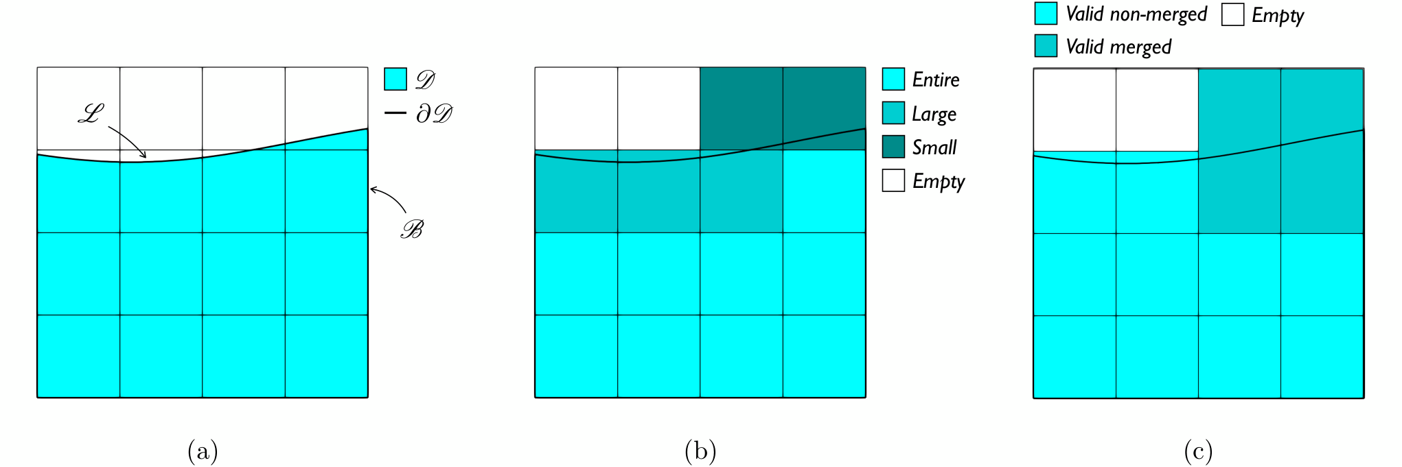
Let $\mathscr{D}$ be the domain, which we assume to be enclosed in a background rectangle $\mathscr{R}\supseteq\mathscr{D}$. We then let $\Phi:\mathscr{R}\rightarrow\mathbb{R}$ be a level set function such that $\mathscr{D}$ is implicitly defined as the region where $\Phi$ is negative, i.e. $\mathscr{D}\equiv\{\boldsymbol{x}\in\mathscr{R}:\Phi(\boldsymbol{x})<0\}$, and its boundary $\partial\mathscr{D}$ is defined as $\partial\mathscr{D}\equiv\mathscr{B}\cup\mathscr{L}$, where $\mathscr{B}\equiv\{\boldsymbol{x}\in\partial\mathscr{R}:\Phi(\boldsymbol{x})<0\}$ is the portion of the rectangle’s outer boundary $\partial\mathscr{R}$ where $\Phi$ is negative, and $\mathscr{L}\equiv\{\boldsymbol{x}\in\mathscr{R}:\Phi(\boldsymbol{x})=0\}$ is the zero level of $\Phi$. We then introduce a structured grid $\mathscr{G}_{h}\equiv\cup_{\boldsymbol{i}}\mathscr{C}^{\boldsymbol{i}}\subseteq\mathscr{R}$, where $h$ denotes a characteristic mesh size, $\mathscr{C}^{\boldsymbol{i}}$ is a generic rectangular cell and $\boldsymbol{i}\equiv\{i_{k}\}$ is the $d$-tuple identifying the location of the cell within the grid. The cell $\mathscr{C}^{\boldsymbol{i}}$ is defined as $[x_{1}^{\boldsymbol{i}},x_{1}^{\boldsymbol{i}}+h_{1}]\times\dots\times[x_{d}^{\boldsymbol{i}},x_{d}^{\boldsymbol{i}}+h_{d}]$, where $x_{k}^{\boldsymbol{i}}$ is the cell’s lower corner in the $k$-th direction and $h_{k}$ is the grid’s mesh size in that direction.

When intersected with the domain $\mathscr{D}$, cells are characterized by their volume fraction $\nu$: entire cells fall entirely inside $\mathscr{D}$ and have volume fraction $\nu=1$; empty cells fall entirely outside $\mathscr{D}$ and have volume fraction $\nu=0$; partial cells are cut by $\mathscr{L}$ and have volume fraction $0<\nu<1$. We then introduce a volume fraction threshold $\overline{\nu}$ to label each partial cell as either large if $\overline{\nu}<\nu<1$ or small if $0<\nu\leq\overline{\nu}$. As an example, Fig.(1a) shows a two-dimensional domain embedded in a $4\times 4$ grid and Fig.(1b) shows the corresponding cell classification.

The volume fraction threshold triggers the cell-merging strategy, whereby all cells labelled as small are merged with nearby cells. Several possibilities exist for implementing the cell-merging strategy. Here, a small cell is merged with one of its entire or large neighboring cells, henceforth collectively referred to as valid cells. The neighbor targeted for merging is selected according to its location with respect to the small cell and its volume fraction. Specifically, neighboring cells are queried in the following order: in 3D, we first consider the set of valid cells sharing a face with the small cell, second we consider the set of valid cells sharing an edge with the small cell and finally we consider the set of valid cells sharing a corner with the small cell. Within each set, the neighbors are ordered according to their volume fraction. Then, the target neighbor is the first cell in the first non-empty set. It follows that, in the choice of the target neighbor, a large cell sharing a face with the small cell has higher priority than an entire cell sharing an edge with the small cell. In 2D, the search starts from the cells that share an edge with a small cell.

Once the cell-merging procedure is applied, the cells of the grid $\mathscr{G}_{h}$ consist of valid non-merged cells, i.e. the entire and large cells that have not been targeted during the merging process, valid merged cells, i.e. the union of small cells and their merging large or entire neighbors, and empty cells. Such a classification for the background cells of Fig.(1b) is shown in Fig.(1c). Then, the implicitly-defined mesh $\mathcal{M}_{h}$ associated with $\mathscr{G}_{h}$ is defined by the intersection of the valid merged and non-merged cells of $\mathscr{G}_{h}$ and the domain $\mathscr{D}$, such that $\mathcal{M}_{h}\equiv\{\mathscr{D}^{e}\}$ and $\mathscr{D}^{e}$ is the $e$-th implicitly-defined mesh element. Figure (2) shows the implicitly-defined mesh associated with the grid of Fig.(1c) and highlights (in darker color) an implicitly-defined element $\mathscr{D}^{e}$ resulting from the merging of a small cell and an entire cell. The figure also shows the outer boundaries $\mathscr{B}^{e}$ and $\mathscr{L}^{e}$ of the $e$-th element, which stem from the intersection of the grid with $\mathscr{B}$ and $\mathscr{L}$, respectively, and the internal boundaries $\mathscr{I}^{e,e^{\prime}}$ that the $e$-th element shares with its generic neighboring element $e^{\prime}$. A few comments are worth pointing out:

• •

  In the implementation of the implicit mesh, we do not explicitly merge cells. When a small cell and a valid cell have been merged, both the dG and the reconstructed FV representations of the solution on that merged cell are specified in terms of coefficients associated with the valid cell. Moreover, the geometry of the curved elements is never explicitly constructed or parameterized and is only inferred by the quadrature rules for domains and boundaries implicitly defined by the level set function.

• •

  The cell-merging procedure needs to traverses the cells only once and is fully parallelizable. In fact, the volume fraction of the cells is computed prior to and does not change during the merging process; for example, after being merged, a small cell does not become a large cell eligible for merging with another small cell. Each small cell queries its neighboring cells and selects the most appropriate neighbor according to the procedure described above. Note that multiple small cells can target the same cell for merging; as a 2D example, Fig.(3a) shows a 4$\times$4 grid where the small cells $\mathscr{C}^{4,3}$, $\mathscr{C}^{3,4}$ and $\mathscr{C}^{4,4}$ all merge with the cell $\mathscr{C}^{3,3}$ to define the implicitly-defined mesh element $\mathscr{D}^{e}$. A similar example in 3D is shown in Fig.(3b).

• •

  In general, and especially for high volume fraction thresholds, it is possible that the merging algorithm does not find a suitable neighbor, i.e., given a small cell, all the cells in its 3$\times$3 (in 2D) or its 3$\times$3$\times$3 (in 3D) neighborhood are small or empty; if this occurs, the simulation will terminate and require a smaller volume fraction threshold. However, in all the numerical tests considered here, a volume fraction threshold of 0.3 in 2D and a volume fraction threshold of 0.15 in 3D was found to be satisfactory. Other approaches could be implemented to deal with small cells that do not find suitable neighbors for merging. For example, one could consider merging multiple small cells together, thus increasing the effective mesh size of the elements, or one could lower the volume fraction threshold that triggers the merging and introduce an additional higher volume fraction thresholds that instead triggers a reduced polynomial order representation, thus improving the stability of the scheme. These approaches are, however, not considered here.

Discontinuous Galerkin schemes are based on a weak form of the governing equations. For each element in the mesh we define a local polynomial basis on that element and extend it to vanish on all of the other elements. The collection of these functions for each element then forms a discontinuous basis. Here, it is natural to define the local basis functions as tensor-product polynomials since the discretization is constructed using Cartesian grids and the majority of the mesh elements are rectangular cells.

Let $\mathscr{D}^{e}$ be the implicitly-defined element associated with the grid cell $\mathscr{C}^{\boldsymbol{i}}$ (and all the small cells that are merged with $\mathscr{C}^{\boldsymbol{i}}$) and let $\mathcal{P}_{hp}^{e}$ be the space of tensor-product polynomials of degree $p$ in the rectangular domain occupied by $\mathscr{C}^{\boldsymbol{i}}$. Then, the space $\mathcal{V}_{hp}$ of discontinuous basis functions for the mesh $\mathcal{M}_{h}$ based on the grid $\mathscr{G}_{h}$ is

while the related space $\mathcal{V}_{hp}^{N}$ of discontinuous polynomials vector fields is $\mathcal{V}_{hp}^{N}\equiv(\mathcal{V}_{hp})^{N}$.

Following Cockburn et al.[29, 30], we integrate by parts in space to obtain the weak form of Eq.(1) as

In Eq.(5), $\mathcal{N}^{e}$ denotes the set of mesh elements that are neighbors of $\mathscr{D}^{e}$, and $\widehat{\boldsymbol{F}}_{n}$ denotes the so-called numerical flux, whose expression for hyperbolic equations is typically computed using an exact or an approximate Riemann solver [55, 56].

We now approximate $\boldsymbol{U}$ on each element as a linear combination of basis functions with time dependent coefficients. This can be written compactly as

where $\boldsymbol{B}^{e}$ is an $N_{u}\times N_{u}N_{p}$ matrix where each column corresponds to a basis function in $\mathcal{V}_{hp}$ and $\boldsymbol{X}^{e}(t)$ is a vector of coefficients of length $N_{u}N_{p}$. Here $N_{u}=d+2$ is the number of unknowns in the system and $N_{p}=(1+p)^{d}$ is the number of polynomials in $\mathcal{P}_{hp}^{e}$. Substituting Eq. (6) into Eq.(5) and letting $\boldsymbol{V}$ range over the basis functions, we obtain the final semidiscrete evolution equation

where the superimposed dot denotes the derivative with respect to time, and $\boldsymbol{M}^{e}$ is the mass matrix of $e$-th element given by

The domain and boundary integrals appearing in Eqs.(7) and (8) are evaluated using high-order quadrature rules for implicitly-defined domains and boundaries. These quadrature rules are generated using the algorithm developed by Saye [54] and provide high-order accuracy in the presence of smooth embedded geometries. This is a key ingredient for the accuracy of the overall scheme. For example, Qin and Krivodonova [6] discuss the importance of an accurate representation of embedded geometries and use curvature-aware boundary conditions to avoid the loss of accuracy due to the piecewise representation of the embedded boundaries. An example of the quadrature rules used here is provided in Fig.(4), which shows the distribution of the quadrature points for the domain and boundary integrals of 2D and 3D implicitly-defined elements.

In a FV setting, the weak form of the governing equations can be derived by integrating Eq.(1) over a generic implicitly-defined element $\mathscr{D}^{e}\in\mathcal{M}_{h}$ and applying the divergence theorem with respect to the space variables to obtain

where the superimposed dot again denotes the derivative with respect to time, $m^{e}\equiv\int_{\mathscr{D}^{e}}1~\mathrm{d}{V}$ is the volume of $\mathscr{D}^{e}$, $\boldsymbol{U}^{e}$ represents the average of the conserved variables over $\mathscr{D}^{e}$, i.e. $\boldsymbol{U}^{e}\equiv\frac{1}{m^{e}}\int_{\mathscr{D}^{e}}\boldsymbol{U}\mathrm{d}{V}$, and the remaining symbols have the same meaning as those appearing in Eq.(5).

Similar to Eq.(7), high-order quadrature rules are employed to evaluate the right-hand side of Eq.(9) and maintain the high-order accuracy representation of the geometry for the FV scheme. However, unlike dG schemes, where the solution at any space location within the element is computed via its polynomial representation, Eq.(9) requires a suitable reconstruction and limiting strategy, which allows one to evaluate the solution, and thus the numerical flux $\widehat{\boldsymbol{F}}_{n}$, at the element’s boundaries.

Although high-order reconstruction methods are available in the literature, the present approach is based on a linear representation of the solution, which leads to a scheme that is at most second-order accurate in space. This choice is mainly motivated by the fact that, within the adaptive mesh refinement algorithm, the FV grids will be fine-tuned to track and resolve the regions containing solution discontinuities, where high-order schemes would be reduced to first-order schemes by the limiter. The details of the limiter employed here are given in Sec.(3.3.1).

The dG schemes and FV schemes are integrated into a block-structured adaptive mesh refinement algorithm (AMR) [60, 61, 62] that represents the solution as a hierarchy of levels of refinement ranging from coarsest ($\ell=0$) to finest ($\ell={\ell}_{\rm finest}$). Each level is represented by the union of non-overlapping logically-rectangular grids of a given resolution.

Here, the grids at level $\ell=0$ are generated at the beginning of the simulation and cover the entire domain; the corresponding implicitly-defined mesh is also generated at startup and does not change during the simulation. Grids at levels $\ell>0$ are created and destroyed dynamically during the simulation, and the corresponding implicitly-defined meshes follow the same dynamic evolution. We consider AMR configurations where dG schemes are used at the levels $0\leq\ell<{\ell}_{\rm finest}$ while the FV scheme is always used at the finest level $\ell={\ell}_{\rm finest}$. This includes the case where AMR uses dG schemes only or the case where AMR consists of a single-level FV scheme. The present AMR strategy also supports the use of different order basis functions at different dG levels and, as such, is referred to as $hp$-AMR. Figure (6) shows an example of a 3-level $hp$-AMR configuration with a refinement ratio of 4 between level 0 and level 1 and a refinement ratio of 2 between level 1 and level 2. The figure also shows that dG schemes are used at levels 0 and 1 and a FV scheme is used at the level 2. This configuration is typical of what one would expect for a discontinuity attached to a curved boundary.

The dynamic update of the AMR levels is governed by tagging and un-tagging operations, whereby a cell at a given level is assigned a two-value variable, or tag, that determines whether a finer resolution is required at its location or whether the existing set of finer grid cells can be replaced by a coarse cell. These operations require coarsening and refinement operations that transfer the solution between levels. For instance, when a coarse cell is tagged for refinement and a finer grid is overlaid on it, the solution from the coarse level needs to be interpolated to the newly created fine grid. Conversely, the solution at a fine level must be restricted to the corresponding coarser level to determine whether or not the fine grid is still required at that location. These operations must preserve the high-order accuracy of the method and must be available for all the possible combinations of the numerical schemes used between consecutive levels. Nevertheless, these are linear operations local to elements and therefore can be efficiently implemented using matrix-vector products taking advantage of parallelization offered by dG and FV schemes.

To illustrate how interpolation and restriction are performed here, we introduce the vector $\boldsymbol{X}_{\ell}$ of the solution at the level $\ell$. For a level that uses a dG scheme, $\boldsymbol{X}_{\ell}$ contains the coefficients of the basis functions representing the conserved variables, whereas, for a level that uses the FV scheme, $\boldsymbol{X}_{\ell}$ collects the element averages of the conserved variables. For the interpolation and restriction operations, we consider the FV scheme as a dG scheme of discontinuous constant basis functions. This means that interpolation to the finest level returns the element averages, which are subsequently used to perform the reconstruction and limiting process presented in Sec.(3.3.1). Note that interpolation is never performed from the finest level and therefore the reconstructed slopes are not used during the interpolation and restriction operations.

As sketched in Fig.(7a), the interpolation operator $\boldsymbol{I}_{\ell+1,\ell}$ computes the solution $\boldsymbol{X}_{\ell+1}$ at the fine level $\ell+1$ from the solution $\boldsymbol{X}_{\ell}$ at the coarse level $\ell$, and is formally written as

In Eq.(19), $\boldsymbol{I}_{\ell+1,\ell}$ is a block-structured matrix computed using a Galerkin projection, so that, given an element $\mathscr{D}_{\ell+1}^{e^{\prime}}$ of the fine level $\ell+1$ and an element $\mathscr{D}_{\ell}^{e}$ of the coarse level $\ell$ for which the interpolation operation is meaningful, the block $\boldsymbol{I}_{\ell+1,\ell}^{e^{\prime},e}$ is given by

where, for an element $e$ on level $\ell$, $\boldsymbol{B}_{\ell}^{e}$ contains the basis functions and $\boldsymbol{M}_{\ell}^{e}$ is the mass matrix as defined in Eq.(8).

It is worth giving a practical example of how the interpolation operator $\boldsymbol{I}_{\ell+1,\ell}$ acts on $\boldsymbol{X}_{\ell}$. Consider Fig.(7b), which shows a two-element coarse mesh $\mathcal{M}_{h_{\ell}}\equiv\{\mathscr{D}_{\ell}^{1},\mathscr{D}_{\ell}^{2}\}$ associated with a $1\times 2$ coarse grid, and a five-element fine mesh $\mathcal{M}_{h_{\ell+1}}\equiv\{\mathscr{D}_{\ell+1}^{1},\mathscr{D}_{\ell+1}^{2},\dots,\mathscr{D}_{\ell+1}^{5}\}$ associated with a $2\times 4$ grid that is obtained by refining the coarse grid with a refinement ratio of 2. Then, $\boldsymbol{X}_{\ell}$ consists of the basis functions coefficients of the elements $\mathscr{D}_{\ell}^{1}$ and $\mathscr{D}_{\ell}^{2}$, $\boldsymbol{X}_{\ell+1}$ consists of the basis functions coefficients of the elements $\mathscr{D}_{\ell+1}^{1}$ to $\mathscr{D}_{\ell+1}^{5}$. The interpolation operation given in Eq.(19) becomes

where each block $\boldsymbol{I}_{\ell+1,\ell}^{e,e^{\prime}}$, with $e=1,\dots,5$ and $e^{\prime}=1,2$, is computed via Eq.(20). While the first, second, third and fifth rows of Eq.(21) are the result of a trivial application of the Galerkin projection, it is interesting to derive the interpolation operation given in the fourth row of Eq.(21). First, with reference to Fig.(7b), note that the fine element $\mathscr{D}_{\ell+1}^{4}$ is the result of a merging operation and covers portions of the two distinct coarse elements $\mathscr{D}_{\ell}^{1}$ and $\mathscr{D}_{\ell}^{2}$. Then, assuming for simplicity that $\boldsymbol{X}_{\ell}$ contains the basis functions coefficients of a discontinuous scalar field $u:\mathcal{M}_{h_{\ell}}\rightarrow\mathbb{R}$ at the coarse level $\ell$, the Galerkin projection of $u$ onto the fine element $\mathscr{D}_{\ell+1}^{4}$ is given by

where the last equality is obtained by noting that $\mathscr{D}_{\ell+1}^{4^{\prime}}\equiv\mathscr{D}_{\ell+1}^{4}\cap\mathscr{D}_{\ell}^{1}$ and $\mathscr{D}_{\ell+1}^{4^{\prime\prime}}\equiv\mathscr{D}_{\ell+1}^{4}\cap\mathscr{D}_{\ell}^{2}$, and by using Eq.(20). The structure of $\boldsymbol{I}_{\ell+1,\ell}$ given in Eq.(21) reflects the configurations of the coarse and the fine meshes displayed in Fig.(7b), including the merging between cells; moreover, if $\mathscr{D}_{\ell+1}^{e^{\prime}}\cap\mathscr{D}_{\ell}^{e}=\emptyset$, then the corresponding block $\boldsymbol{I}_{\ell+1,\ell}^{e,e^{\prime}}$ is a zero matrix.

Figure (7b) also sketches the inverse of the interpolation operation, namely the restriction operation, where a solution $\boldsymbol{X}_{\ell}$ at a coarse level $\ell$ is computed from the solution $\boldsymbol{X}_{\ell+1}$ at a fine level $\ell+1$ using the restriction operator $\boldsymbol{R}_{\ell,\ell+1}$

Following Fortunato et al.[63], the restriction operator can be defined as the adjoint of the interpolation operator and can evaluated as follows

where $\boldsymbol{M}_{\ell}$ denotes the block-diagonal mass matrix associated to the entire level $\ell$, i.e. $\boldsymbol{M}_{\ell}\equiv\mathrm{diag}(\{\boldsymbol{M}_{\ell}^{e}\})$. Note that Eq.(24) can also be obtained by applying the Galerkin projection from the fine level $\ell+1$ onto the coarse level $\ell$ and using Eq.(20). For the case shown in Fig.(7b), Eq.(24) becomes

A few comments are worth pointing out:

• •

  The interpolation and restriction operators defined via Eqs.(20) and (23), respectively, are valid regardless of the choice of basis functions and can accommodate AMR levels using different mesh sizes, polynomial orders or both. In particular, they are valid even if the same mesh uses the same space of basis functions with different polynomial orders; this feature will be used to define the shock sensor discussed in Sec.(3.4.1).

• •

  From an implementation perspective, given an $hp$-AMR configuration, one only needs to evaluate the interpolation operators and the Cholesky decomposition of the mass matrices; then the restriction operator can be applied on-the-fly using Eq.(24). Moreover, all the standard rectangular elements (which represent most of the mesh elements) share the same mass matrix, which can precomputed and stored at the beginning of the simulation; the same applies to the interpolation operator between two standard rectangular elements of two different AMR levels. For the remaining implicitly-defined mesh elements, the mass matrices and the interpolation operators are in general unique and are computed using high-order quadrature rules [54].

• •

  The mass matrix and interpolation operator are formally given by $\boldsymbol{M}_{\ell}$ and $\boldsymbol{I}_{\ell+1,\ell}$ that dynamically change as the $hp$-AMR levels evolve. However, these matrices are composed of localized blocks that can be computed and stored after each regridding.

• •

  The interpolation and restriction operations are well-defined in all configurations of the implicitly-defined mesh obtained from the cell-merging algorithm as long as tagged cells are not merged with non-tagged cells. This situation can always be avoided by making sure that if an extended cell is tagged for refinement, so are all the small cells merged with it.

As the last comment on the present $hp$-AMR strategy, recall that when the right-hand side of Eq.(7) or (9) is to be evaluated, the coupling between neighboring elements $e$ and $e^{\prime}$ occurs solely through the numerical flux $\widehat{\boldsymbol{F}}_{n}$ appearing in the boundary integrals over $\mathscr{I}^{e,e^{\prime}}$. This applies equally to the cases when $e$ and $e^{\prime}$ belong to the same $hp$-AMR level or when $e$ and $e^{\prime}$ belong to different $hp$-AMR levels, including the level using the FV scheme. In fact, at a generic quadrature point $\boldsymbol{x}$ of $\mathscr{I}^{e,e^{\prime}}$, $\widehat{\boldsymbol{F}}_{n}$ is computed as $\widehat{\boldsymbol{F}}_{n}=\widehat{\boldsymbol{F}}_{n}(\widetilde{\boldsymbol{U}}{}^{e},\widetilde{\boldsymbol{U}}{}^{e^{\prime}})$, where $\widetilde{\boldsymbol{U}}{}^{e}$ is the solution evaluated at $\boldsymbol{x}$ using either its representation in terms of basis functions, if the element $e$ belongs to a level using a dG scheme, or the reconstruction provided by Eq.(10), if the element $e$ belongs to a level using the FV scheme. However, is it pointed out that at the boundary between two levels using different schemes, the order of the quadrature rules must be high enough to provide an accurate integration of the contributions from the higher-order scheme.

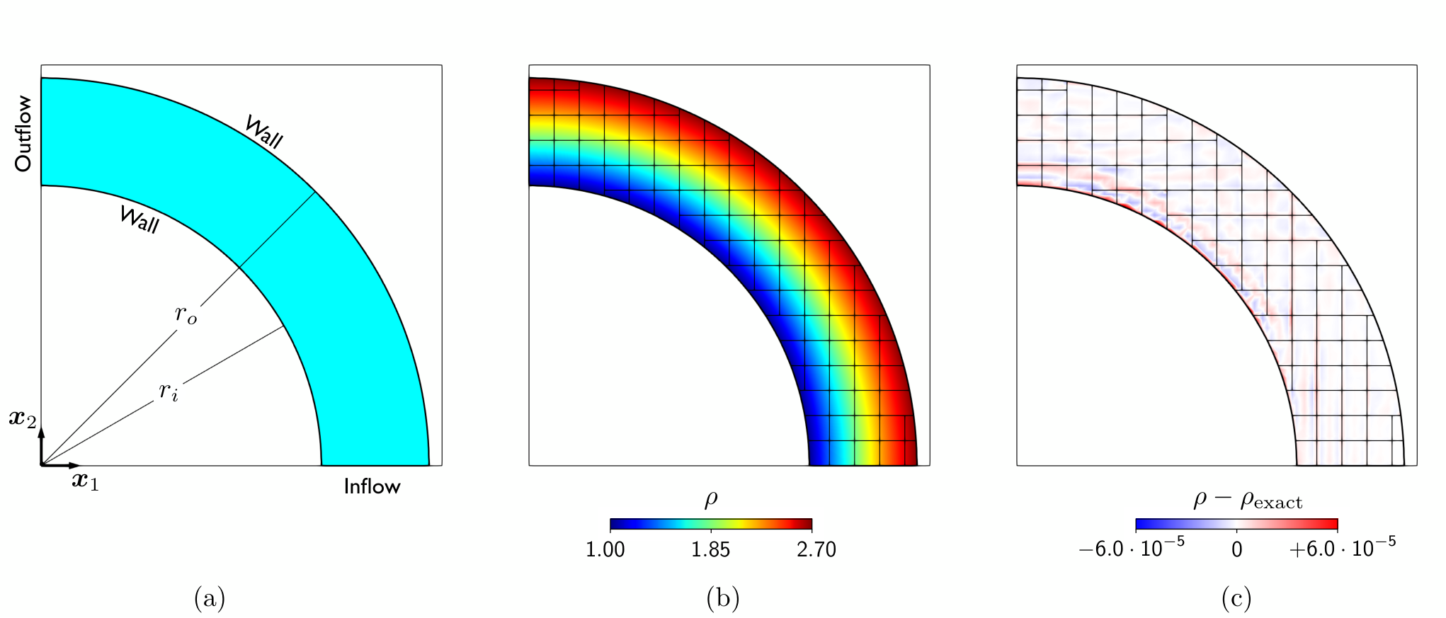
In this test, we consider a two-dimensional supersonic vortex problem with an exact smooth solution that has been employed in several studies to investigate the accuracy of numerical methods for inviscid gas dynamics, see e.g. [64, 28]. The problem consists of isentropic flow in a circular annulus of inner radius $r_{i}=1$ and outer radius $r_{o}=1.384$. The exact solution for density $\rho_{\mathrm{exact}}$, pressure $p_{\mathrm{exact}}$, and velocity components $v_{1\mathrm{exact}}$ and $v_{2\mathrm{exact}}$ are given by the following expressions

where $v_{\theta}=a_{i}M_{i}\frac{r_{i}}{r}$, $r$ is the distance between a point inside the annulus and the center of the annulus, and $\rho_{i}=1$, $a_{i}=1$ and $M_{i}=2.25$ are the density, sound speed and Mach number, respectively, at $r=r_{i}$.

The problem is defined in the background square $\mathscr{R}=[0,1.43]^{2}$ where the domain $\mathscr{D}$ and its boundaries are represented by the level set function

Figure (8a) shows the geometry of the problem and indicates the boundary conditions. The exact solution given in Eq.(31) is used to define the initial conditions for Eq.(29). The system is integrated in time until a steady state is reached. We consider two error measures

where $||\cdot||_{2}$ and $||\cdot||_{\infty}$ are the standard $L_{2}(\mathscr{D})$ norm and $L_{\infty}(\mathscr{D})$ norm, respectively, defined on the domain $\mathscr{D}$, $\rho$ is the value computed using the present approach and $\rho_{\mathrm{exact}}$ is given by Eq.(31). The steady-state solution is assumed to be reached when the relative error between the evaluation of the norms given in Eq.(33) between two consecutive time steps is less than 10^-5. For all considered simulations, this occurred at $t>5.0$.

The simulations are performed using a single-level mesh, with $h\equiv 1.43/n$, where $n$ is the number of elements per side of the background square, and where the volume fraction threshold $\overline{\nu}=0.3$. Figure (8b) shows the density distribution obtained using a $16\times 16$ background mesh and a dG₃ scheme; the corresponding density error distribution is reported in fig.(8c), which also shows that the maximum error is observed near the inner boundary of the annulus. The error measures defined in Eq.(33) are shown in Fig.(9) as functions of the numerical scheme and the mesh size $h$. As seen in the figures, the dG schemes show an $\mathcal{O}(h^{p+1})$ convergence rate in the $L_{2}$ norm and an $\mathcal{O}(h^{p+1/2})$ convergence rate in the $L_{\infty}$ norm, while the FV scheme using the reconstruction (without limiting) presented in Sec.(3.3.1) obtains the same convergence rate as the dG₁ scheme, albeit with a slightly larger error.

In the second test, we consider Sod’s shock tube problem in embedded geometries. These simulations assess the ability of the implicitly-defined mesh and the reconstruction and limiting technique presented in Sec.(3.3.1) to reproduce a one-dimensional flow within a geometry that is not aligned with the background grid.

The problem is defined in the background unit cube $\mathscr{R}=[0,1]^{d}$ as shown in Fig.(10). In 2D, the tube is a strip of width $2r$ centered at $\boldsymbol{c}\equiv\{0.5,0.5\}$ whose orientation is defined by the parameter $\theta$, which denotes the inclination of the tube’s centerline. In 3D, the tube is a cylinder with a circular cross section of radius $r$ centered at $\boldsymbol{c}\equiv\{0.5,0.5,0.5\}$ whose orientation is defined by the two parameters $\theta$ and $\phi$, which denote the azimuth and the elevation, respectively, of the tube’s centerline. For convenience, we introduce a rotated coordinate system $\hat{\boldsymbol{\xi}}\hat{\boldsymbol{\eta}}$ (in 2D) or $\hat{\boldsymbol{\xi}}\hat{\boldsymbol{\eta}}\hat{\boldsymbol{\zeta}}$ (in 3D) centered in $\boldsymbol{c}$, where $\hat{\boldsymbol{\xi}}$ is aligned with the tube’s centerline and the unit vectors have the following components

in 2D or 3D, respectively. Then, a convenient way to represent the domain and its boundaries is through the level set function $\boldsymbol{\Phi}(\boldsymbol{x})\equiv\eta^{2}-r^{2}$ in 2D, or $\boldsymbol{\Phi}(\boldsymbol{x})\equiv\eta^{2}+\zeta^{2}-r^{2}$ in 3D, where $\xi$, $\eta$ and $\zeta$ are the components of $\boldsymbol{x}$ in the rotated coordinate system.

The initial conditions are given by

and the final time is $T=0.2$. Wall boundary conditions are prescribed along the embedded boundaries. At the intersection between the domain and the background cube’s boundary, ghost states with the initial conditions are prescribed at the quadrature points.

The solution to Sod’s shock tube problem consists of three waves: a rarefaction wave, a contact discontinuity and a shock wave. To account for the presence of the discontinuities, a two-level mesh is employed. Level $\ell=0$ is obtained by subdividing the background domain into $64^{d}$ cells and uses a dG₂ scheme. Level $\ell=1$ is constructed using a refinement ratio of 4 and is dynamically updated from level 0 using the shock sensor described in Sec.(3.4.1). Specifically, at time $t$, the smoothness indicator $s^{e}$ given in Eq.(27) is computed for each element of the implicitly-defined mesh at level 0; then, the elements satisfying the condition (28) are tagged for refinement to level 1. In Eq.(28), $\kappa_{s}=-2.00$ for the 2D problem and $\kappa_{s}=-2.45$ for the 3D problem. Finally, the implicitly-defined mesh is generated using volume fraction thresholds $\overline{\nu}_{0}=\overline{\nu}_{1}=0.3$ in 2D and $\overline{\nu}_{0}=\overline{\nu}_{1}=0.15$ in 3D. It is worth pointing out that the implicitly-defined elements are simple polygons in 2D, whereas they have curved surfaces in 3D. However, as shown in the results, this will have very little effect on the computed numerical solutions.

The top row of images in Fig.(11) shows the density distribution at times $t=0$, $t=0.04$ and $t=0.20$ for the 2D tube corresponding to the orientation $\theta=30^{\circ}$. The bottom row of images in Fig.(11) shows the density distribution at the same times for the 3D tube corresponding to the orientation $\theta=60^{\circ}$ and $\phi=30^{\circ}$. In 3D, the density distribution is represented by isosurfaces of $\rho=\{0.15,0.3,0.6,0.7,0.8,0.9\}$, which allow us to see the rarefaction wave, the contact discontinuity and the shock along the tube. Figure (11) also displays the evolution of the mesh level using the FV scheme, whose location is identified by the stepped black lines. The figure shows that the FV level tracks the shock discontinuity but not the contact discontinuity. Although it is possible to adjust the constant $\kappa_{s}$ in (28) in such a way as to make the FV level track the contact discontinuities, numerical experiments show that these discontinuities are only temporarily tracked by the FV scheme and, once they are sufficiently smoothed, they stop satisfying the condition (28) and start being tracked by the unlimited dG scheme. This is an expected behavior since shocks steepen while contact discontinuities do not.

The robustness of the proposed approach is tested by considering four orientations each in 2D and 3D while keeping the same settings for the implicitly-defined mesh and the shock sensor. Figure (12) shows the results at the final time $t=0.2$ for orientation angles $\theta=0^{\circ}$, $30^{\circ}$, $45^{\circ}$ and $60^{\circ}$, in 2D, and for orientation angles $\{\theta,\phi\}=\{0^{\circ},0^{\circ}\}$, $\{0^{\circ},30^{\circ}\}$, $\{45^{\circ},60^{\circ}\}$ and $\{60^{\circ},30^{\circ}\}$, in 3D. The first row shows the density distribution for the four 2D configurations, the second row shows the corresponding pressure distribution, the third row shows the density distribution for the four 3D configurations and the fourth row shows the corresponding pressure. For the 3D cases, the density distribution is represented by isosurfaces of $\rho=\{0.15,0.3,0.6,0.7,0.8,0.9\}$ while the pressure distribution is represented by isosurfaces of $p=\{0.15,0.6,0.7,0.8,0.9\}$. For all configurations, the coupled dG-FV scheme is able to reproduce the one-dimensional flow in embedded curved geometries that are not aligned with the background grid. This can be seen more clearly by looking at line plots of the density and pressure distribution along the centerline and the wall for the embedded shock tubes at the final time $t=0.2$. Figures (13a), (13b), (13c) and (13d) show the density along the centerline, the pressure along the centerline, the density along the wall and the pressure along the wall, respectively, as functions of the local reference system coordinate $\xi$ and the 2D tube’s orientation. Similarly, Figs.(14a), (14b), (14c) and (14d) show the same quantities as functions of the local reference system coordinate $\xi$ and the 3D tube’s orientation. As seen in the figures, the rarefaction wave, the contact discontinuity and the shock wave are all well captured by the proposed approach and match the one-dimensional solution well, regardless of the orientation of the embedded geometry. Moreover, the numerical results in the tilted geometries are nearly indistinguishable from the numerical results in the aligned geometry, which can be viewed as a reference solution where the implicitly-defined mesh has little effect.

Finally, we note in Fig.(10), the wall values in 2D are those computed at $\eta=r$, i.e. at the upper embedded boundary of the tube, whereas the wall values in 3D are those computed at $\eta=\zeta=\tilde{r}\equiv r/\sqrt{2}$, i.e. at one line on the embedded boundary of the tube. Similar results are observed if the wall values are evaluated at other boundary locations.

In the third test, we consider a shock reflection from a cylinder in 2D and a shock reflection from a sphere in 3D. These problems have been investigated experimentally [65] and allow us to assess the capabilities of numerical methods to capture the shock structure as well as the details of the smooth flow patterns.

Shock reflection from a cylinder in 2D is defined in the background unit square $\mathscr{R}=[0,1]^{2}$. The geometry is represented by the level set function $\Phi(\boldsymbol{x})\equiv r^{2}-(x_{k}-c_{k})(x_{k}-c_{k})$ where $\boldsymbol{c}=\{0.5,0.5\}$ and $r=0.1$ are the center and the radius of the cylinder, respectively as shown in Fig.(15a). The shock is initially located at $x_{1}=d_{s}=0.2$ and travels towards the cylinder at a mach number $M=2.81$. The initial conditions are given by

References

- Aftosmis et al. [2000] Aftosmis, M., Berger, M., and Adomavicius, G. A parallel multilevel method for adaptively refined cartesian grids with embedded boundaries. In 38th Aerospace Sciences Meeting and Exhibit, page 808, 2000.
- Peskin [2002] Peskin, C. S. The immersed boundary method. Acta numerica, 11:479–517, 2002.
- Mokbel et al. [2018] Mokbel, D., Abels, H., and Aland, S. A phase-field model for fluid–structure interaction. Journal of Computational Physics, 372:823–840, 2018.
- Kemm et al. [2020] Kemm, F., Gaburro, E., Thein, F., and Dumbser, M. A simple diffuse interface approach for compressible flows around moving solids of arbitrary shape based on a reduced baer–nunziato model. Computers & Fluids, 204:104536, 2020.
- Moës et al. [1999] Moës, N., Dolbow, J., and Belytschko, T. A finite element method for crack growth without remeshing. International journal for numerical methods in engineering, 46(1):131–150, 1999.
- Qin and Krivodonova [2013] Qin, R. and Krivodonova, L. A discontinuous galerkin method for solutions of the euler equations on cartesian grids with embedded geometries. Journal of Computational Science, 4(1-2):24–35, 2013.
- Alauzet et al. [2016] Alauzet, F., Fabrèges, B., Fernández, M. A., and Landajuela, M. Nitsche-xfem for the coupling of an incompressible fluid with immersed thin-walled structures. Computer Methods in Applied Mechanics and Engineering, 301:300–335, 2016.
- Saye [2017a] Saye, R. Implicit mesh discontinuous galerkin methods and interfacial gauge methods for high-order accurate interface dynamics, with applications to surface tension dynamics, rigid body fluid–structure interaction, and free surface flow: Part i. Journal of Computational Physics, 344:647–682, 2017a.
- Saye [2017b] Saye, R. Implicit mesh discontinuous galerkin methods and interfacial gauge methods for high-order accurate interface dynamics, with applications to surface tension dynamics, rigid body fluid–structure interaction, and free surface flow: Part ii. Journal of Computational Physics, 344:683–723, 2017b.
- Milazzo et al. [2018] Milazzo, A., Benedetti, I., and Gulizzi, V. An extended ritz formulation for buckling and post-buckling analysis of cracked multilayered plates. Composite Structures, 201:980–994, 2018.
- Berger [2017] Berger, M. Cut cells: Meshes and solvers. In Handbook of Numerical Analysis, volume 18, pages 1–22. Elsevier, 2017.
- LeVeque et al. [2002] LeVeque, R. J. et al. Finite volume methods for hyperbolic problems, volume 31. Cambridge university press, 2002.
- Versteeg and Malalasekera [2007] Versteeg, H. K. and Malalasekera, W. An introduction to computational fluid dynamics: the finite volume method. Pearson education, 2007.
- Clarke et al. [1986] Clarke, D. K., Salas, M., and Hassan, H. Euler calculations for multielement airfoils using cartesian grids. AIAA journal, 24(3):353–358, 1986.
- Gaffney and Hassan [1987] Gaffney, JR, R. and Hassan, H. Euler calculations for wings using cartesian grids. In 25th AIAA Aerospace Sciences Meeting, page 356, 1987.
- Hartmann et al. [2008] Hartmann, D., Meinke, M., and Schröder, W. An adaptive multilevel multigrid formulation for cartesian hierarchical grid methods. Computers & Fluids, 37(9):1103–1125, 2008.
- Ji et al. [2010] Ji, H., Lien, F.-S., and Yee, E. Numerical simulation of detonation using an adaptive cartesian cut-cell method combined with a cell-merging technique. Computers & fluids, 39(6):1041–1057, 2010.
- Hartmann et al. [2011] Hartmann, D., Meinke, M., and Schröder, W. A strictly conservative cartesian cut-cell method for compressible viscous flows on adaptive grids. Computer Methods in Applied Mechanics and Engineering, 200(9-12):1038–1052, 2011.
- Cecere and Giacomazzi [2014] Cecere, D. and Giacomazzi, E. An immersed volume method for large eddy simulation of compressible flows using a staggered-grid approach. Computer Methods in Applied Mechanics and Engineering, 280:1–27, 2014.
- Muralidharan and Menon [2016] Muralidharan, B. and Menon, S. A high-order adaptive cartesian cut-cell method for simulation of compressible viscous flow over immersed bodies. Journal of Computational Physics, 321:342–368, 2016.
- Pember et al. [1995] Pember, R. B., Bell, J. B., Colella, P., Curtchfield, W. Y., and Welcome, M. L. An adaptive cartesian grid method for unsteady compressible flow in irregular regions. Journal of computational Physics, 120(2):278–304, 1995.
- Almgren et al. [1997] Almgren, A. S., Bell, J. B., Colella, P., and Marthaler, T. A cartesian grid projection method for the incompressible euler equations in complex geometries. SIAM Journal on Scientific Computing, 18(5):1289–1309, 1997.
- Colella et al. [2006] Colella, P., Graves, D. T., Keen, B. J., and Modiano, D. A cartesian grid embedded boundary method for hyperbolic conservation laws. Journal of Computational Physics, 211(1):347–366, 2006.
- Graves et al. [2013] Graves, D., Colella, P., Modiano, D., Johnson, J., Sjogreen, B., and Gao, X. A cartesian grid embedded boundary method for the compressible navier–stokes equations. Communications in Applied Mathematics and Computational Science, 8(1):99–122, 2013.
- Helzel et al. [2005] Helzel, C., Berger, M. J., and LeVeque, R. J. A high-resolution rotated grid method for conservation laws with embedded geometries. SIAM Journal on Scientific Computing, 26(3):785–809, 2005.
- Berger and Helzel [2012] Berger, M. and Helzel, C. A simplified h-box method for embedded boundary grids. SIAM Journal on Scientific Computing, 34(2):A861–A888, 2012.
- Gokhale et al. [2018] Gokhale, N., Nikiforakis, N., and Klein, R. A dimensionally split cartesian cut cell method for hyperbolic conservation laws. Journal of Computational Physics, 364:186–208, 2018.
- Berger and Giuliani [2021] Berger, M. and Giuliani, A. A state redistribution algorithm for finite volume schemes on cut cell meshes. Journal of Computational Physics, 428:109820, 2021.
- Cockburn et al. [1990] Cockburn, B., Hou, S., and Shu, C.-W. The runge-kutta local projection discontinuous galerkin finite element method for conservation laws. iv. the multidimensional case. Mathematics of Computation, 54(190):545–581, 1990.
- Cockburn and Shu [1998] Cockburn, B. and Shu, C.-W. The runge–kutta discontinuous galerkin method for conservation laws v: multidimensional systems. Journal of Computational Physics, 141(2):199–224, 1998.
- Arnold et al. [2002] Arnold, D. N., Brezzi, F., Cockburn, B., and Marini, L. D. Unified analysis of discontinuous galerkin methods for elliptic problems. SIAM journal on numerical analysis, 39(5):1749–1779, 2002.
- Cockburn [2018] Cockburn, B. Discontinuous galerkin methods for computational fluid dynamics. Encyclopedia of Computational Mechanics Second Edition, pages 1–63, 2018.
- Cangiani et al. [2017] Cangiani, A., Dong, Z., and Georgoulis, E. H. hp-version space-time discontinuous galerkin methods for parabolic problems on prismatic meshes. SIAM Journal on Scientific Computing, 39(4):A1251–A1279, 2017.
- Antonietti and Pennesi [2019] Antonietti, P. F. and Pennesi, G. V-cycle multigrid algorithms for discontinuous galerkin methods on non-nested polytopic meshes. Journal of Scientific Computing, 78(1):625–652, 2019.
- Bastian and Engwer [2009] Bastian, P. and Engwer, C. An unfitted finite element method using discontinuous galerkin. International journal for numerical methods in engineering, 79(12):1557–1576, 2009.
- Johansson and Larson [2013] Johansson, A. and Larson, M. G. A high order discontinuous galerkin nitsche method for elliptic problems with fictitious boundary. Numerische Mathematik, 123(4):607–628, 2013.
- Brandstetter and Govindjee [2015] Brandstetter, G. and Govindjee, S. A high-order immersed boundary discontinuous-galerkin method for poisson’s equation with discontinuous coefficients and singular sources. International Journal for Numerical Methods in Engineering, 101(11):847–869, 2015.
- Gürkan and Massing [2019] Gürkan, C. and Massing, A. A stabilized cut discontinuous galerkin framework for elliptic boundary value and interface problems. Computer Methods in Applied Mechanics and Engineering, 348:466–499, 2019.
- Lew and Buscaglia [2008] Lew, A. J. and Buscaglia, G. C. A discontinuous-galerkin-based immersed boundary method. International Journal for Numerical Methods in Engineering, 76(4):427–454, 2008.
- Heimann et al. [2013] Heimann, F., Engwer, C., Ippisch, O., and Bastian, P. An unfitted interior penalty discontinuous galerkin method for incompressible navier–stokes two-phase flow. International Journal for Numerical Methods in Fluids, 71(3):269–293, 2013.
- Kummer [2017] Kummer, F. Extended discontinuous galerkin methods for two-phase flows: the spatial discretization. International Journal for Numerical Methods in Engineering, 109(2):259–289, 2017.
- Krause and Kummer [2017] Krause, D. and Kummer, F. An incompressible immersed boundary solver for moving body flows using a cut cell discontinuous galerkin method. Computers & Fluids, 153:118–129, 2017.
- Saye [2020] Saye, R. Fast multigrid solution of high-order accurate multiphase stokes problems. Communications in Applied Mathematics and Computational Science, 15(2):147–196, 2020.
- Gulizzi et al. [2020a] Gulizzi, V., Benedetti, I., and Milazzo, A. An implicit mesh discontinuous galerkin formulation for higher-order plate theories. Mechanics of Advanced Materials and Structures, 27(17):1494–1508, 2020a.
- Gulizzi et al. [2020b] Gulizzi, V., Benedetti, I., and Milazzo, A. A high-resolution layer-wise discontinuous galerkin formulation for multilayered composite plates. Composite Structures, 242:112137, 2020b.
- Müller et al. [2017] Müller, B., Krämer-Eis, S., Kummer, F., and Oberlack, M. A high-order discontinuous galerkin method for compressible flows with immersed boundaries. International Journal for Numerical Methods in Engineering, 110(1):3–30, 2017.
- Geisenhofer et al. [2019] Geisenhofer, M., Kummer, F., and Müller, B. A discontinuous galerkin immersed boundary solver for compressible flows: Adaptive local time stepping for artificial viscosity–based shock-capturing on cut cells. International Journal for Numerical Methods in Fluids, 91(9):448–472, 2019.
- Fidkowski and Darmofal [2007] Fidkowski, K. J. and Darmofal, D. L. A triangular cut-cell adaptive method for high-order discretizations of the compressible navier–stokes equations. Journal of Computational Physics, 225(2):1653–1672, 2007.
- Xiao et al. [2019] Xiao, H., Febrianto, E., Zhang, Q., and Cirak, F. An immersed discontinuous galerkin method for compressible navier-stokes equations on unstructured meshes. International Journal for Numerical Methods in Fluids, 91(10):487–508, 2019.
- Persson and Peraire [2006] Persson, P.-O. and Peraire, J. Sub-cell shock capturing for discontinuous galerkin methods. In 44th AIAA Aerospace Sciences Meeting and Exhibit, page 112, 2006.
- Chaudhuri et al. [2017] Chaudhuri, A., Jacobs, G. B., Don, W.-S., Abbassi, H., and Mashayek, F. Explicit discontinuous spectral element method with entropy generation based artificial viscosity for shocked viscous flows. Journal of Computational Physics, 332:99–117, 2017.
- Krivodonova [2007] Krivodonova, L. Limiters for high-order discontinuous galerkin methods. Journal of Computational Physics, 226(1):879–896, 2007.
- Zahr et al. [2020] Zahr, M. J., Shi, A., and Persson, P.-O. Implicit shock tracking using an optimization-based high-order discontinuous galerkin method. Journal of Computational Physics, 410:109385, 2020.
- Saye [2015] Saye, R. High-order quadrature methods for implicitly defined surfaces and volumes in hyperrectangles. SIAM Journal on Scientific Computing, 37(2):A993–A1019, 2015.
- Colella and Glaz [1985] Colella, P. and Glaz, H. M. Efficient solution algorithms for the riemann problem for real gases. Journal of Computational Physics, 59(2):264–289, 1985.
- Toro [2013] Toro, E. F. Riemann solvers and numerical methods for fluid dynamics: a practical introduction. Springer Science & Business Media, 2013.
- Van Leer [1979] Van Leer, B. Towards the ultimate conservative difference scheme. v. a second-order sequel to godunov’s method. Journal of computational Physics, 32(1):101–136, 1979.
- Berger et al. [2005] Berger, M., Aftosmis, M., and Muman, S. Analysis of slope limiters on irregular grids. In 43rd AIAA Aerospace Sciences Meeting and Exhibit, page 490, 2005.
- Barth and Jespersen [1989] Barth, T. and Jespersen, D. The design and application of upwind schemes on unstructured meshes. In 27th Aerospace sciences meeting, page 366, 1989.
- Berger and Colella [1989] Berger, M. J. and Colella, P. Local adaptive mesh refinement for shock hydrodynamics. Journal of computational Physics, 82(1):64–84, 1989.
- Bell et al. [1994] Bell, J., Berger, M., Saltzman, J., and Welcome, M. Three-dimensional adaptive mesh refinement for hyperbolic conservation laws. SIAM Journal on Scientific Computing, 15(1):127–138, 1994.
- Zhang et al. [2019] Zhang, W., Almgren, A., Beckner, V., Bell, J., Blaschke, J., Chan, C., Day, M., Friesen, B., Gott, K., Graves, D., et al. Amrex: a framework for block-structured adaptive mesh refinement. Journal of Open Source Software, 4(37):1370–1370, 2019.
- Fortunato et al. [2019] Fortunato, D., Rycroft, C. H., and Saye, R. Efficient operator-coarsening multigrid schemes for local discontinuous galerkin methods. SIAM Journal on Scientific Computing, 41(6):A3913–A3937, 2019.
- Krivodonova and Berger [2006] Krivodonova, L. and Berger, M. High-order accurate implementation of solid wall boundary conditions in curved geometries. Journal of computational physics, 211(2):492–512, 2006.
- Bryson and Gross [1961] Bryson, A. and Gross, R. Diffraction of strong shocks by cones, cylinders, and spheres. Journal of Fluid Mechanics, 10(1):1–16, 1961.
- Ram et al. [2015] Ram, O., Geva, M., and Sadot, O. High spatial and temporal resolution study of shock wave reflection over a coupled convex–concave cylindrical surface. Journal of Fluid Mechanics, 768:219–239, 2015.
- Soni et al. [2017] Soni, V., Hadjadj, A., Chaudhuri, A., and Ben-Dor, G. Shock-wave reflections over double-concave cylindrical reflectors. Journal of Fluid Mechanics, 813:70, 2017.
- Koronio et al. [2020] Koronio, E., Ben-Dor, G., Sadot, O., and Geva, M. Similarity in mach stem evolution and termination in unsteady shock-wave reflection. Journal of Fluid Mechanics, 902, 2020.
- Krivodonova et al. [2004] Krivodonova, L., Xin, J., Remacle, J.-F., Chevaugeon, N., and Flaherty, J. E. Shock detection and limiting with discontinuous galerkin methods for hyperbolic conservation laws. Applied Numerical Mathematics, 48(3-4):323–338, 2004.
- Klöckner et al. [2011] Klöckner, A., Warburton, T., and Hesthaven, J. S. Viscous shock capturing in a time-explicit discontinuous galerkin method. Mathematical Modelling of Natural Phenomena, 6(3):57–83, 2011.
- Lv et al. [2016] Lv, Y., See, Y. C., and Ihme, M. An entropy-residual shock detector for solving conservation laws using high-order discontinuous galerkin methods. Journal of Computational Physics, 322:448–472, 2016.
- Fernandez et al. [2018] Fernandez, P., Nguyen, C., and Peraire, J. A physics-based shock capturing method for unsteady laminar and turbulent flows. In 2018 AIAA Aerospace Sciences Meeting, page 0062, 2018.
- Clain et al. [2011] Clain, S., Diot, S., and Loubère, R. A high-order finite volume method for systems of conservation laws—multi-dimensional optimal order detection (mood). Journal of computational Physics, 230(10):4028–4050, 2011.
- Dumbser et al. [2014] Dumbser, M., Zanotti, O., Loubère, R., and Diot, S. A posteriori subcell limiting of the discontinuous galerkin finite element method for hyperbolic conservation laws. Journal of Computational Physics, 278:47–75, 2014.
- Zanotti et al. [2015] Zanotti, O., Fambri, F., Dumbser, M., and Hidalgo, A. Space–time adaptive ader discontinuous galerkin finite element schemes with a posteriori sub-cell finite volume limiting. Computers & Fluids, 118:204–224, 2015.
- Minion [2004] Minion, M. L. Semi-implicit projection methods for incompressible flow based on spectral deferred corrections. Applied numerical mathematics, 48(3-4):369–387, 2004.
- Almgren et al. [2013] Almgren, A. S., Aspden, A., Bell, J. B., and Minion, M. L. On the use of higher-order projection methods for incompressible turbulent flow. SIAM Journal on Scientific Computing, 35(1):B25–B42, 2013.
- Minion and Saye [2018] Minion, M. L. and Saye, R. Higher-order temporal integration for the incompressible navier–stokes equations in bounded domains. Journal of Computational Physics, 375:797–822, 2018.
- Titarev and Toro [2002] Titarev, V. A. and Toro, E. F. Ader: Arbitrary high order godunov approach. Journal of Scientific Computing, 17(1):609–618, 2002.
- Balsara et al. [2013] Balsara, D. S., Meyer, C., Dumbser, M., Du, H., and Xu, Z. Efficient implementation of ader schemes for euler and magnetohydrodynamical flows on structured meshes–speed comparisons with runge–kutta methods. Journal of Computational Physics, 235:934–969, 2013.