Stability and Super-resolution of MUSIC and ESPRIT for Multi-snapshot Spectral Estimation
Abstract
This paper studies the spectral estimation problem of estimating the locations of a fixed number of point sources given multiple snapshots of Fourier measurements collected by a uniform array of sensors. We prove novel stability bounds for MUSIC and ESPRIT as a function of the noise standard deviation, number of snapshots, source amplitudes, and support. Our most general result is a perturbation bound of the signal space in terms of the minimum singular value of Fourier matrices. When the point sources are located in several separated clumps, we provide an explicit upper bound of the noise-space correlation perturbation error in MUSIC and the support error in ESPRIT in terms of a Super-Resolution Factor (SRF). The upper bound for ESPRIT is then compared with a new Cramér-Rao lower bound for the clumps model. As a result, we show that ESPRIT is comparable to that of the optimal unbiased estimator(s) in terms of the dependence on noise, number of snapshots and SRF. As a byproduct of our analysis, we discover several fundamental differences between the single-snapshot and multi-snapshot problems. Our theory is validated by numerical experiments.
Index Terms:
Multi-snapshot spectral estimation, stability, super-resolution, MUSIC algorithm, optimality of ESPRIT algorithm, Cramér-Rao lower bound, array imaging.I Introduction
I-A Problem formulation and motivation
This paper studies the spectral estimation problem of estimating the locations of a fixed number of point sources given multiple time snapshots of Fourier measurements collected by a uniform array of sensors. Let be the number of point sources which we assume are located in the set , where is the torus. We denote the source amplitudes at time by the complex-valued vector . At time , a uniform array of sensors collects a noisy measurement vector
| (I.1) |
where is the Fourier sensing matrix with entries
for and and represents a noise vector at time . The sensing matrix only depends on and , and is independent of time . It does not necessarily contain orthogonal columns unless is a subset of .
Typically in practice, samples of are collected at times and each is called a snapshot. This paper studies the multi-snapshot spectral estimation problem of estimating the source locations from these snapshots: . This problem appears in many interesting imaging and signal processing applications, including inverse scattering [15], Direction-Of-Arrival (DOA) estimation [22, 45, 38] and spectral analysis [48].
Various methods have been developed by the imaging and signal processing communities for multi-snapshot spectral estimation [40, 45, 44, 20, 1]. A class of algorithms commonly referred to as subspace methods are widely used in applications due to their impressive empirical performance, especially in the context of super-resolution imaging where some point sources are close together. In particular, MUSIC [45] and ESPRIT [44] are among the most popular subspace methods. MUSIC and ESPRIT are applicable in multi-dimensions as well [43]. The success of MUSIC and ESPRIT has been demonstrated in many simulations and applications [53].
Despite great developments in numerical methods and extensive empirical studies, there are many open theoretical questions regarding the stability and super-resolution of subspace methods. This paper focuses on the fundamental performance analysis question: What is the stability of MUSIC and ESPRIT, as a function of the noise standard deviation, the number of snapshots, source amplitudes, and the support set?
Prior theoretical work on related super-resolution problems [13, 31, 30] suggest that the stability of the multi-snapshot spectral estimation problem crucially depends on the locations of the point sources. The minimum separation of is
where . Since consecutive Fourier coefficients are collected during each time snapshot, the standard imaging resolution is , which is referred to as the Rayleigh Length (RL) in optics [10].
We expect the stability of this problem to be different depending on the relationship between and . In this article, we are particularly interested in is the super-resolution regime where , so that there exist and whose distance is smaller than 1 RL. When this is the case, we define the super-resolution factor (SRF) by
| (I.2) |
I-B Main results
The main contribution of this paper is a detailed performance analysis of MUSIC and ESPRIT in terms of the fundamental model quantities: the number of snapshots, noise standard deviation, support set, and source amplitudes.
- (a)
Our most general upper bounds for the perturbation of MUSIC (Theorem IV.5) and ESPRIT (Theorem IV.6) show that their average errors can be controlled by a term that is linear in
(I.3) where Noise represents the noise standard deviation to be specified in Assumption (II.1), denotes the -th largest singular value of , and is the minimum eigenvalue of the amplitude covariance matrix to be defined in (II.1). This inequality not only captures the correct dependence on the number of snapshots and noise, but it also highlights how the stability of both algorithms implicitly depends on the configuration of the support set through the quantity .
- (b)
To give a more transparent upper bound in the super-resolution regime, we consider a specific scenario where consists of separated clumps and the point sources in each clump can be close together. Our upper bounds for the stability of MUSIC (Theorem V.3) and ESPRIT (Theorem V.4) are proportional to
where is the cardinality of the largest clump. This indicates that, for challenging super-resolution problems where is large, additional snapshots or higher quality samples must be taken for compensation.
- (c)
We prove a new Cramér-Rao lower bound (Theorem VI.3) under a specific separated clumps model in Theorem VI.3. This lower bound matches our upper bound for ESPRIT in terms of the dependence on noise, and , thereby certifying that the performance of ESPRIT is comparable to that of the optimal unbiased estimator(s) for this model.
I-C Comparison and connection to other works
Prior resolution analysis of subspace methods for multi-snapshot spectral estimation [58, 16, 41] focused on a special case where there are only two closely spaced point sources. The papers [58, 16] analyzed the probability that two sources are correctly detected instead of being misspecified as a single source. It was shown in [41] that the ESPRIT support error is upper bounded by a term on the order of for certain Signal-to-Noise Ratio (SNR) defined in the referenced article.
To our knowledge, there are no other theoretical works that address more complicated situations beyond two closely spaced point sources, e.g., when the support contains multiple clumps of point sources and the point sources in each clump can be closely spaced. A theoretical analysis for more complicated situations could be valuable. For example, a recent article [34] empirically compared the performance of several numerical methods, including MUSIC, for DOA estimation of several point sources arranged in complicated ways. Other models have been considered, see [9, 57], but this direction is beyond the scope of this work.
In literature, many existing works have addressed the sensitivity of multi-snapshot MUSIC [17, 52, 28, 18] and ESPRIT [51, 28, 37]. Many of these works focus on sensitivity to model errors, which arise from antenna array perturbations, sensor gain and phase errors, diagonal noise covariance perturbations, etc. A first-order perturbation analysis is given in [17, 52, 28, 27, 18, 41] for MUSIC, in [51, 28, 37] for ESPRIT, in [43] for tensor-ESPRIT in the multidimensional case, and in [12] for the estimation of a damped complex exponential. The results in [27, 41, 43] and many others prove that, the sensitivity of MUSIC and ESPRIT is proportional to Noise. However, they are implicit for a super-resolution analysis since the dependence on SRF is often hidden in some matrix eigenvalue.
When MUSIC and ESPRIT are used in applications, many interesting techniques have been developed to improve its performance. Spatial smoothing [39, 42, 46] is widely used when some sources are coherent, or if only a small number of snapshots is available. A first-order perturbation analysis with spatial smoothing is given in [39, 42] and in [46] in the multi-dimensional case. When the source amplitudes are non-circular, some analysis can be found in [46]. Mathematical theories on the sensitivity of MUSIC and ESPRIT usually assume that the number of sources is known. In practice, an accurate estimation of is an interesting problem. We refer to [59, 55, 23, 33, 56] for some interesting techniques and statistical analysis on the estimation of .
The classical Cramér-Rao Bound (CRB) [8] provided a lower bound on the variance of any unbiased estimator of the support, and was extensively investigated in [49, 50, 26, 21]. The paper that is most relevant to us is [26], which gave a Cramér-Rao lower bound when all point sources are almost equally spaced in a small interval. This result is summarized in detail in Section VI-A.
In recent years, spectral estimation has been extensively studied in the single-snapshot scenario where , and primarily from a deterministic viewpoint. Performance guarantees of a convex optimization algorithm were established in [6, 14] for sufficiently separated point sources and in [36, 4] for super-resolution. On the other hand, MUSIC and ESPRIT are non-convex methods, and their stability and super-resolution limits were addressed in [30, 29, 31]. A detailed review for the single-snapshot setting can be found in [30]. There are fundamental differences between the single-snapshot and multi-snapshot problems, which we discuss in Section VIII. Due to these differences, the results in this paper can not be directly deduced from the ones in [30, 29, 31].
I-D Organization
This paper is organized as follows. We introduce assumptions and define important terminology in Section II. We define the signal space associated with this problem and derive an error between the true and empirical signal spaces in Section III. We present our stability analysis for MUSIC and ESPRIT in Section IV, and then consider a separated clumps model in Section V. To understand the fundamental limits of spectral estimation, we deduce a new Cramér-Rao lower bound under a specific separated clumps model in Section VI and compare it to our upper bound for ESPRIT. We present numerical experiments in Section VII and discuss the differences between the multi-snapshot versus single-snapshot problems in Section VIII. All proofs are contained in Section XI.
I-E Notation
We use and to denote the set of real and complex numbers respectively. For , we denote its angle by . For a vector , we denote the diagonal matrix with on the diagonal by . We let denote the Euclidean norm of and be its conjugate transpose. Let be the identity matrix and be the Kronecker delta; that is, if , and if .
For a matrix , we use to denote the singular values of listed in non-increasing order, and each singular value appears according to its multiplicity. If has real eigenvalues, we use to denote its eigenvalues of . We use and for the spectral and Frobenius norms of , respectively. Let be the conjugate transpose of . We use to denote the Hadamard (pointwise) product of two matrices of equal size. For a linear operator , we denote its range by . For any subspace , we let be the orthogonal projection onto . Slightly abusing notation, we let be the orthogonal projection onto .
We use to specify that is a random variable such that , , and for all . For a complex , we write to mean that the real and imaginary parts are independent random variables. If is an event, then denotes its complement and is the indicator function of .
We use the notation to mean that there exists a depending only on such that .
Throughout the paper, we assume that the noise vectors are random, and the expectation is taken over the probability distribution of the noise .
II Assumptions and covariance matrices
Our performance guarantees for MUSIC and ESPRIT require the following standard assumptions.
Assumption II.1.
(Model assumptions) Fix positive integers such that and .
- (a)
has cardinality and does not depend on .
- (b)
The amplitude covariance matrix,
(II.1) is strictly positive-definite.
- (c)
There exist such that for any , the entries of are independent complex random variables. For , assume and are independent. These assumptions imply that
- (d)
For each , we are given
- (e)
The noise level satisfies the following assumption
(II.2)
Assumption II.1 is standard in spectral and DOA estimations [45, 22, 49]. This assumption can be justified as follows:
Assumption II.1(a) is necessary from a statistical viewpoint. If is allowed to change over time, then there might be no relationship between and for , so collecting additional snapshots might not be beneficial. Under this assumption, is a special type of matrix, often referred to as a non-harmonic Fourier matrix or Vandermonde matrix with nodes on the complex unit circle, and by the celebrated Vandermonde determinant theorem, has rank and .
Assumption II.1(b) on the strictly positive-definiteness of the amplitude covariance matrix is standard in array imaging and DOA estimation [45, 22, 49]. This assumption is equivalent to the requirement that span . If this assumption is void, both MUSIC and ESPRIT can be modified as the single-snapshot scenario by utilizing a Hankel structure. This is a technical point to be discussed in Section VIII.
For example, Assumption II.1(b) can be used in models where evolves over time according to a physical law. Many stochastic models of fulfill Assumption II.1(b). For instance, if are independent Gaussian vectors with i.i.d. entries, then has full rank with probability one. More generally, if is sub-Gaussian and the population covariance of is strictly positive-definite, then has full rank with high probability, see [54][Theorem 4.71 and Exercise 4.7.3].
When snapshots of measurements are taken, we define the matrices
| (II.3) | ||||
The empirical covariance matrices are
| (II.4) | ||||
| (II.5) |
Defining , one can verify that
| (II.6) |
III Signal space and its empirical estimation
III-A Signal and noise space
A signal space plays an important role in a class of subspace methods [22], including MUSIC and ESPRIT. These algorithms first compute an empirical version of the signal space by a truncated eigen-decomposition, and then extract the source locations based on this signal space.
Definition III.1 (Signal and noise spaces).
The signal space is defined to be the column space of , and the noise space is defined to be the orthogonal complement of the signal space.
Although the signal and noise spaces do not depend on the specific choice of orthonormal basis, we pick particular bases purely for convenience. Throughout this paper, we let and such that and be matrices whose columns form an orthonormal basis for the signal space and the noise space, respectively. Due to identity (II.6) and Assumption II.1(b), the signal space is the eigenspace associated with the largest eigenvalues of .
With snapshots of noisy measurements, the signal and noise spaces can be estimated from the empirical covariance matrix as follows. Let be a unitary matrix whose columns are eigenvectors of , and the columns of are the eigenvectors corresponding to the largest eigenvalues of .
Definition III.2.
We refer to and as the empirical signal space and the empirical noise space, respectively.
III-B An accurate perturbation bound for the signal space
In this paper, we establish an accurate perturbation bound for . Roughly speaking, if the number of snapshots is sufficiently large, and everything else is fixed, the empirical signal space is a good approximation of the signal space . We first quantify the distance between and by their canonical angles.
Definition III.3.
Suppose and . The canonical angles between and are defined to be , for . Let
The (Euclidean) distance between and is
| (III.1) |
This definition extends the notion of an angle between two vectors to subspaces, and it is invariant to the particular choice of basis. It follows from [47, Chapter I, Theorem 5.5] and [7, Lemma 2.1.2] that
| (III.2) | ||||
It is a consequence of [58, Theorem 3] that the distance between and satisfies the following expectation bound. See Section XI-A for the details.
Theorem III.4.
Under Assumption II.1, there exists a constant depending only on such that
Remark III.5.
Note that defined in (II.1) is normalized by , so we can interpret has a normalized quantity. Since has columns each with Euclidean norm , we can also interpret as a normalized quantity. Hence, Theorem III.4 tells us that the average squared distance between and tends to zero proportional (at least) linearly in .
Remark III.6.
Throughout this paper, we will provide upper bounds for the average squared distance. We can use Jensen’s inequality, to convert them into an upper bound for the expected error if desired.
IV Stability of MUSIC and ESPRIT
IV-A Review of MUSIC and ESPRIT
In signal processing, MUSIC [45] and ESPRIT [44] have been widely used in applications due to their impressive numerical performance and super-resolution phenomenon.
We first introduce some important notations. We define the signal vector at as
The columns of in (I.1) exactly consist of the signal vectors at the sources locations:
In the noiseless situation, MUSIC amounts to finding the noise space, forming the noise-space correlation function and identifying the zero set of the noise-space correlation, which is necessarily the support set. When , we have the following observations regarding the Vandermonde matrix :
- •
- •
if and only if .
These observations imply that, if and only if . Since the signal space is exactly , the condition of can be quantified by a noise-space correlation function or an imaging function.
Definition IV.1 (Noise-space correlation (NSC) and imaging functions).
For any , the noise-space correlation function is defined as
The imaging function is defined as
The MUSIC algorithm is based on the following lemma:
Lemma IV.2.
Let . Then
Lemma IV.2 implies that, the source locations can be exactly identified through the roots of the noise-space correlation function, or the peaks of the imaging function.
When snapshots of noisy measurements are taken, we can compute the empirical signal space .
Definition IV.3 (Empirical NSC and imaging functions).
For any , the empirical noise-space correlation (NSC) function is defined to be
The empirical imaging function is defined to be
An estimate for the support set is obtained by extracting the largest local maxima of , or equivalently, the smallest local minima of . MUSIC is summarized in Algorithm 1.
ESPRIT reformulates the support estimation step as an eigenvalue problem. We first discuss the noiseless situation. By definition, the signal space is the column space of , and so there exists an invertible matrix such that Let and be two submatrices of containing the first and the last rows respectively. Denote as the submatrix containing the first rows of . Letting , we have
Setting guarantees that and have rank . It follows that
Hence, the eigenvalues of are exactly . The ESPRIT algorithm amounts to finding the support set through the eigenvalues of .
When snapshots of noisy measurements are taken, ESPRIT follows the same steps but with the empirical signal space instead of . It is summarized in Algorithm 1.
To quantify the error between and , we introduce the support matching distance.
Definition IV.4.
The matching distance between and is
where is a permutation on .
IV-B Stability of MUSIC and ESPRIT
The stability of MUSIC depends on the perturbation of the NSC function from to , which can be measured as
Theorem IV.5.
Unlike MUSIC, ESPRIT is an explicit algorithm since it reformulates the main question as an eigenvalue problem. For ESPRIT, we have the following estimate for the matching distance between the true and recovered support.
Theorem IV.6.
Due to the considerable length of the proof of Theorem IV.6, we split the proof into two parts. Parts (a) and (b) are proved in Sections XI-C and XI-D respectively. Part (a) holds for all possible values of and . On the other hand, part (b) requires that (which can be interpreted as a scaled and squared signal-to-noise-ratio) is sufficiently large depending on the model parameters.
V Super-resolution of multi-snapshot MUSIC and ESPRIT
V-A Minimum singular value of Fourier matrices
In this section, we consider a general model of where the point sources are clustered into separated clumps.
Assumption V.1.
(Separated clumps model). Let and be a positive integers and have cardinality We say that consists of separated clumps with parameters if the following hold.
- (a)
can be written as the union of disjoint sets where each is contained in an interval of length .
- (b)
with where is the cardinality of .
- (c)
If then the distance between any two clumps is at least .
An example of separated clumps is given in Figure 1. There are many types of discrete sets that consist of separated clumps. Extreme examples include when is a single clump containing all points, and when consists of clumps containing a single point. While our theory applies to both extremes, the in-between case where consists of several clumps each of modest size is most interesting. A super-resolution theory of single-snapshot MUSIC and ESPRIT for this separated clumps model is developed in [30, 31, 29]. This paper focuses on the multi-snapshot scenario. The difference between the single-snapshot and multi-snapshot cases is discussed in Section VIII.
Under this separated clumps model, can be estimated as an aggregate of terms, where each term only depends on the “geometry” of each clump [30, Theorem 2.7].
Theorem V.2.
Let . Assume satisfies Assumption V.1 with parameters for some and
| (V.1) |
Then there exist explicit constants where only depends on and such that
An explicit formula for is given in [30, Theorem 2.7, Eq. (2.5)]. In particular, only depends on and (although can be further upper bounded in terms of only if desired) and importantly, does not depend on .
The main feature of this theorem is the exponent on , which depends on the cardinality of each clump as opposed to the total number of points . Let be the cardinality of the largest clump:
| (V.2) |
Since the inequality holds for any that is a set, then it holds for . Defining the super-resolution factor as equation (I.2), Lemma V.2 implies
| (V.3) |
V-B Super-resolution of MUSIC and ESPRIT
In this section, we combine our stability analysis for multi-snapshot MUSIC and ESPRIT in Section IV-B with the minimum singular value estimate in Theorem V.2 to derive a super-resolution theory for multi-snapshot MUSIC and ESPRIT.
For MUSIC, we obtain an upper bound for the perturbation of the noise-space correlation function by combining Theorems IV.5 and V.2.
Theorem V.3.
Theorem V.3 provides a perturbation bound for the noise-space correlation function in multi-snapshot MUSIC under the separated clumps model. The terms that appear in the upper bound in Theorem V.3 can be interpreted as follows: is the noise variance, is the usual stochastic factor, and the quantity in front of can be interpreted as the condition number of super-resolution recovery of multi-snapshot MUSIC. Letting be the cardinality of the largest clump defined in (V.2), Theorem V.3 shows that
| (V.5) |
Notice that the right hand side only depends on the cardinality of the largest clump instead of the total number of point sources . This perturbation bound on MUSIC is verified by numerical experiments in Section VII.
Theorem V.4.
Suppose , satisfies the separated clumps model in Assumption V.1 with parameters such that (V.1) holds. Under Assumption II.1, let and be the constants in Theorems III.4 and V.2 respectively, and let be the output of ESPRIT.
- (a)
Moderate SNR regime. We have
- (b)
Large SNR regime. Define
There is a sufficiently large depending only on such that if
then it holds that
Theorem V.4 provides an estimate of the support error in multi-snapshot ESPRIT under the separated clumps model. Let be the cardinality of the largest clump defined in (V.2). If the assumptions in part (b) hold, then we can provide a simpler estimate,
| (V.6) |
This perturbation bound on ESPRIT is verified by numerical experiments in Section VII.
In comparison, classical perturbation bounds on MUSIC and ESPRIT usually depend on some eigenvalues and eigenvectors of the noiseless covariance matrix , such as (29a, 29b) of [41]. If we know the true source locations and amplitudes, we can compute the eigenvalues and eigenvectors, and then plug them into (29a) of [41]. In real applications, we do not know the true source locations and amplitudes. Therefore, those bounds can not be directly evaluated.
In the special case of two sources, (33a) of [41] shows that the squared source localization error is proportional to ( is referred as the one defined in [41]). The two-source scenario is a special case of our clumps model where the support consists of a single clump with two point sources: and . Therefore, (33a) of [41] is a special case of our Theorem V.3 and Theorem V.4. Our results consider a more general class of support, and such generalization is highly nontrivial.
VI Cramér-Rao lower bound
VI-A Background
The classical Cramér-Rao bound (CRB) [8] expresses a lower bound on the variance of any unbiased estimator of the support . In literature, the Cramér-Rao lower bound has been derived for various models of the support set, and we review some important contributions further below.
Before we proceed, let us recall some old definitions and define some new ones that will be used in this section and Section XI-E. Let .
- •
denotes the vector whose -th entry, for , is .
- •
For each , we let be the vector whose entries are the -th derivative of . Hence, .
- •
For convenience, we let , which will play an important role below.
- •
Given , we let be the matrices whose columns are of the form and , respectively, for each .
The CRB for spectral estimation has been extensively studied [49, 50, 26, 21, 38]. We briefly review some important results. A fundamental result in [49, Theorem 4.1] implies that, under appropriate assumptions, for any unbiased estimator of , not necessarily just MUSIC or ESPRIT, we have
| (VI.1) |
To simplify the notation in this section, we always assume that the elements of have been re-indexed to minimize its matching distance to .
While inequality (VI.1) already gives the optimal dependence on the noise variance and the number of snapshots , the matrix that appears on the right hand side implicitly depends on , so it is unclear how behaves as a function of and . One would hope for an explicit bound depending on the geometry of .
The paper [26] considered a situation where consists of points approximately spaced by . The main result in the aforementioned paper provided an expansion of the right hand side of (VI.1) in the asymptotic limit . In particular, it was shown that
| (VI.2) |
where is independent of but is allowed to depend on the other parameters.
VI-B New CRB for clumps model
The geometric results in Section V, as well as prior work on super-resolution [30], strongly suggest that inequality (VI.2) is unnecessarily pessimistic and is achieved in the worst-case scenario where all point sources are located in a single clump.
This section provides a new CRB for the separated clumps model, under the additional requirements that each clump has elements that are equally spaced by a small parameter . We will derive a CRB on the order of , which is much improved since it is possible that .
We consider a situation where there are clumps that are far apart, and each clump contains points separated by . This is a more specific model than the one considered in Assumption V.1.
Definition VI.1.
We say is a set if and can be written as
Note that this implies consists of disjoint sets each supported in an interval of length and has cardinality .
We also require the following assumptions on the noise and amplitudes.
Assumption VI.2.
Fix any positive integers such that and .
- (a)
Fix and distinct and let be a set.
- (b)
The amplitude covariance matrix is strictly positive-definite.
- (c)
For each and , is a Gaussian random vector with independent entries such that . Also assume that and are independent for .
- (d)
For each , we are given
Theorem VI.3.
Under Assumption VI.2, there exists depending only on , , and such that the following hold. For all , any unbiased estimator of satisfies the lower bound
| (VI.3) |
where the implicit constant does not depend on , , , , and .
VI-C Comparison of our CRB and the classical CRB
In order to explain the main improvement of Theorem VI.3 over classical the CRBs, consider the support set shown in Figure 2. For the depicted in Figure 2, the classical CRB, such as (VI.2), yields the prediction that for any unbiased estimator ,
On the other hand, our CRB in Theorem VI.3 yields
| (VI.5) |
In the super-resolution regime, can be much smaller than , so our CRB provides a significant improvement over the classical CRB.
VI-D Near optimality of ESPRIT
ESPRIT is one of the most popular subspace methods for spectral estimation. To compare our upper bound for ESPRIT and our new CRB, we consider a situation where the assumptions to both Theorems V.4 and VI.3 hold.
- •
- •
Assume that the amplitude covariance matrix is strictly positive-definite.
- •
Assume that for each and , is a Gaussian random vector with independent entries such that . Also assume that and are independent for .
If is sufficiently large so that the assumptions in Theorem V.4 part (b) hold, then the output of ESPRIT satisfies
On the other hand, for any unbiased estimator , Theorem VI.3 and (VI.4) demonstrate that
Notice that these statements are not contradictory since
Thus, we observe that ESPRIT has the same dependence on the noise level , the number of snapshots , and the super-resolution factor compared to the optimal unbiased estimator(s).
VII Numerical experiments
In this section, we perform systematic numerical simulations to validate our theory, under the separated clumps model. We consider the support consisting of clumps of point sources, i.e., . Each clump contains equally spaced points separated by for and respectively. Each amplitude is i.i.d. complex normal such that the real and imaginary parts are independent normal, i.e. . With such amplitudes, . Each noise is an i.i.d. random variable whose real and imaginary parts are independent normal, i.e. . We take snapshots of noisy Fourier measurements according to (I.1). Our upper bounds are proved for the noise-space correlation (NSC) function perturbation in MUSIC and the support error in ESPRIT. When and , we conduct and trials of experiments respectively, and display the average NSC function perturbation in MUSIC and support error in ESPRIT, as well as the standard deviation in Figure 3 - 6. The standard deviation is represented by the error bar.
Our numerical experiments in Figure 3 - 6 are to validate the NSC perturbation in MUSIC and the support error in ESPRIT versus the noise standard deviation , the number of snapshots , and . For MUSIC, the perturbation of the NSC is proved in Theorem IV.5 and Theorem V.3 where the dependence on , , , , can be summarized as:
| (VII.1) |
For ESPRIT, the support error is proved in Theorem IV.6 and Theorem V.4 where the dependence on , , , , in the large SNR regime can be summarized as:
| (VII.2) |
Finally, we show phase transition figures for ESPRIT that validate our perturbation analysis for ESPRIT.
VII-A Error versus Noise
We first test the NSC perturbation in MUSIC and the support error in ESPRIT versus Noise. We set , and for and respectively. Figure 3 (a) shows the NSC perturbation in MUSIC as a function of noise in scale. Figure 3 (b) shows the support error in ESPRIT as a function of noise in scale. The slope for all curves is close to , which demonstrates that the NSC perturbation in MUSIC and the support error in ESPRIT is linear in noise as predicted in (VII.1) and (VII.2).


VII-B Error versus the number of snapshots
We next test the NSC perturbation in MUSIC and the support error in ESPRIT versus the number of snapshots , when and . Figure 4 (a) shows the NSC perturbation in MUSIC as a function of in scale. Figure 4 (b) shows the support error in ESPRIT as a function of in scale. The slope for all curves is close to , which is consistent with (VII.1) and (VII.2).


VII-C Error versus and super-resolution factor (SRF)
Finally we test the NSC perturbation in MUSIC and the support error in ESPRIT versus and SRF respectively, when and . While and are fixed, we vary such that and vary.
Figure 5 (a) shows the NSC perturbation in MUSIC as a function of in scale. Figure 5 (b) shows the support error in ESPRIT as a function of in scale. The slope for all curves is around , which is consistent with (VII.1) and (VII.2).
Figure 6 (a) shows the NSC perturbation in MUSIC as a function of in scale. Figure 6 (b) shows the support error in ESPRIT as a function of in scale. The slope for all curves is around , which is consistent with (VII.1) and (VII.2).


VII-D Phase transition figures for ESPRIT
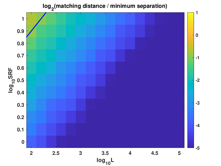
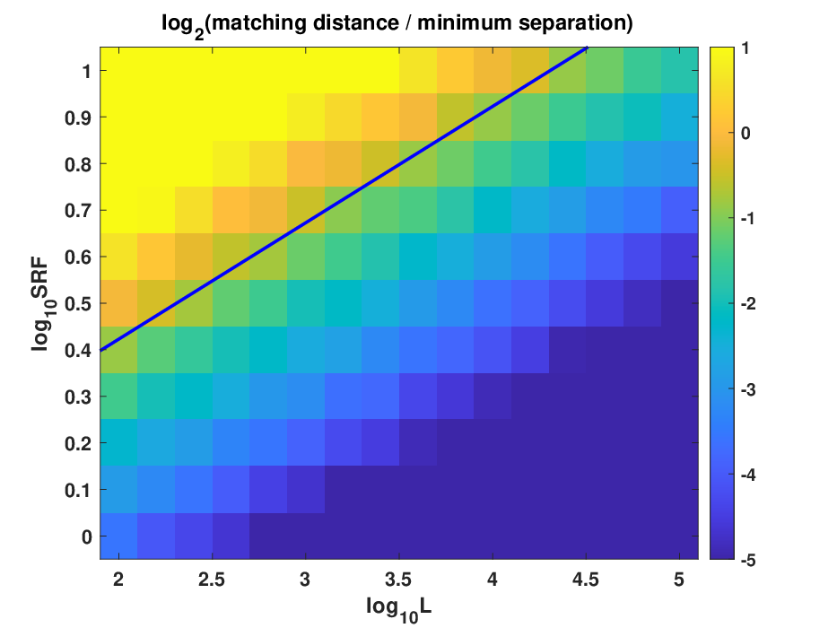
Finally we show the phase transition figures of ESPRIT in Figure 7. Figure 7 shows the average with respect to: (a,b) and when and ; (c,d) and when and ; (e,f) and when and . We observe a clear phase transition phenomenon, and a blue phase transition curve is extracted in each figure. According to (VII.2), we expect the phase transition curve follows
| (VII.3) |
After numerically fitting the phase transition curves, our empirical slope is consistent with our theoretical one in (VII.3).




VIII Multiple versus single snapshot
This paper focuses on the multi-snapshot spectral estimation problem where Fourier measurements of and are collected at different time instances. Since information is collected at different times, it is natural to impose statistical assumptions, which is what we and many other papers have done.
MUSIC and ESPRIT are still applicable for the single-snapshot spectral estimation problem (the case), with proper modification. Instead of forming the empirical covariance matrix in the first step of Algorithm 1, one forms the Hankel matrix of a single-snapshot [32, 31]. From a theoretical perspective, the single-snapshot problem is usually treated from a deterministic point of view.
Single-snapshot MUSIC and ESPRIT enjoy theoretically provable robustness properties in the super-resolution regime, as shown in [30, 31]. The main results there show that for MUSIC and ESPRIT,
| (VIII.1) |
where the implicit constants do not depend on the noise standard deviation , the support set , and . This upper bound matches, up to implicit constants, the minimax lower bounds [30, 2].
A naïve guess is that the error incurred by multi-snapshot MUSIC and ESPRIT would be times that of the single-snapshot setting. Perhaps surprisingly, our results show that this naïve guess is incorrect. Indeed, the main results of this paper for MUSIC (Theorems IV.5 and V.3) and ESPRIT (Theorems IV.6 and V.4) show that on average,
| (VIII.2) |
where again, the implicit constants do not depend on the noise standard deviation , the support set , , and .
Comparing the upper bounds for single-snapshot and multi-snapshot errors, we see that not only does collecting multiple snapshots provide us with the extra cancellation, but it also enjoys an additional square root in the and terms. In other words, the condition numbers of multi-snapshot MUSIC and ESPRIT are significantly better than their single-snapshot counterparts.
The improvement can be explained by the strictly positive-definite assumption on made in Assumption II.1. To see why, consider the deterministic setting where is fixed throughout time, so . Then the collected snapshots are of the form,
Hence, collecting multiple snapshots does not provide us with any new information about the range of since is constant, and the best that can be done is to average all such snapshots,
in order to reduce the variance of the noise by a factor of and feed this averaged signal into single-snapshot MUSIC and ESPRIT. In this highly degenerate situation, the naïve guess for the stability of multi-snapshot MUSIC and ESPRIT is correct.
We also explain how the strictly positive-definite assumption on changes the inherent geometry of the problem. For the sake of this discussion, assume that for all . Since does not change in time, for each . If is strictly positive definite, then spans a -dimensional subspace, so the span of is precisely . On the other hand, if does not have full rank, then only contains partial information about the range of . In which case, multi-snapshot MUSIC and ESPRIT would fail and we would need to use their single-snapshot versions.
IX Conclusion and discussion
This paper analyzes the performance of MUSIC and ESPRIT, and identifies some key quantities that control their stability: number of snapshots, noise variance, amplitude covariance matrix, and the smallest singular value of Fourier matrices (which can then be further estimated in terms of SRF). Our results accurately quantify intuitive phenomenon. For instance, if many point sources are closely spaced then we expect recovery to be sensitive to noise – this is precisely captured by our results since in this case, would be small, and would be large. Likewise if the amplitudes of vary slowly over time, then we expect inversion to be challenging – this is again captured by our results since in that case, would be small and lead to instability. If , then multi-snapshot ESPRIT and MUSIC would fail, but we can instead use their single snapshot versions.
The upper bound for ESPRIT matches a Cramér-Rao lower bound in terms of SRF and max clump cardinality. This proves that no unbiased algorithm can be fundamentally better than ESPRIT for this imaging problem in the large SRF regime – any improvements can only be made in terms of other model parameters such as , , and . These are valuable results for practitioners, as they provide an accurate and solid theoretical footing for discriminating between favorable and unfavorable imaging situations. While this paper only focuses on a one dimensional scenario with plain MUSIC and ESPRIT, we believe the techniques here are also relevant for the analysis of their multi-dimensional counterparts and variations.
X Acknowledgement
All authors would like to thank Zai Yang for finding an error in the first version of this manuscript, and bringing [5] to our attention.
XI Proofs
XI-A Proof of Theorem III.4
Proof.
Recall that . To put this in the framework of [5], we rescale the problem so that
so that now is a matrix with i.i.d. entries. This scaling does not change the singular spaces of and . Applying [5, Theorem 3], which extends to complex matrices without issue, there is a only depending on such that
| (XI.1) |
Since is full rank and assumption (II.2) holds, we have
Using this inequality in (XI.1) completes the proof. ∎
XI-B Proof of Theorem IV.5
XI-C Preparation and proof of Theorem IV.6 part (a)
The stability of ESPRIT relies on several deterministic perturbation results for the perturbation of from , that can be estimated by matrix perturbation theory.
Lemma XI.1.
Suppose and . Then
| (XI.2) |
Proof.
Before we proceed to the stability analysis, we need to point out an important feature of ESPRIT. ESPRIT is invariant to the specific choice of orthonormal basis for the column span of . In other words, the eigenvalues of remain the same if one uses different orthonormal basis for the column space of [31, Section III]. According to [7, Lemma 2.1.3], we can properly choose an orthonormal basis for such that
| (XI.3) |
According to [31, Lemma 3], is lower bounded such that
| (XI.4) |
Combining (XI.3), (XI.4) and the assumption of Lemma XI.1 implies
This enables us to apply [31, Lemma 6], and obtain
We next provide a deterministic bound between and , with [31, Lemma 2].
Lemma XI.2.
On the condition that , the following statements hold:
- (a)
Moderate perturbation regime. We have
- (b)
Small perturbation regime. If additionally,
then
XI-D Preparation and proof of Theorem IV.6 part (b)
We begin by recalling two lemmas, and are essentially immediate consequences of [5].
Lemma XI.3.
Suppose Assumption II.1 holds. Define the events
There exists a sufficiently large depending only on such that the following hold. Suppose
| (XI.6) |
- 1.
There is a depending only on such that
(XI.7) - 2.
There are depending only on such that for all ,
(XI.8)
Proof.
The proof essentially follows from Lemma 4 in the supplement of [5]. For ease of notation, let . To use the mentioned lemma, we first rescale by and take the conjugate transpose of to get,
| (XI.9) |
Notice that the matrix has entries that are i.d.d. random variables. The the right singular vectors of are the left singular vectors of , and the conjugate transpose does not alter the singular values or their ordering.
In this proof, are constants that depend only on , and their values may change from line to line. Now we apply Lemma 4 in the supplement of [5] to (XI.9) to get that, for all ,
| (XI.10) | ||||
For the first bound in (XI.10), we pick
Hence, . The noise condition (II.2) implies that
| (XI.11) |
We also have . So for sufficiently large depending only on (which only depend on ), condition (XI.6) and inequality (XI.11) allow us to say that
| (XI.12) | ||||
Inserting this value of into (XI.10), and using the above observations, we see that
Lemma XI.4.
Suppose Assumption II.1 holds. If , then
Proof of Theorem IV.6 part (b).
In this proof, we let be constants that only depend on . Their values may change from one line to another. Let and be the events defined in Lemma XI.3 and set . Define the event
In this proof, we consider the three events , , and . The first event is a good event where we will be able to apply Lemma XI.1. The third event can be readily controlled using Lemma XI.3. The majority of the proof pertains to the second event , and to do this, we will estimate .
Under event , the inequalities in Lemmas XI.3 imply
This allows us to use Lemma XI.4 when occurs. Using the inequalities in Lemmas XI.3 again, since has orthonormal columns, and from (II.2), under event ,
This inequality implies,
The term can be safely ignored, since by Lemma XI.3 and (IV.2), we have
For sufficiently large depending only on (since the implicit constants in this inequality only depend on ), we have and .
Let us continue with our goal of bounding . We use Lemma XI.4 to see that
Condition (IV.2) implies that , so for sufficiently large , we have
We use the inequality, for all , with and , which is justified by (IV.2), to finally see that
| (XI.13) |
Now we are ready to finish the proof. Recall we have the trivial upper bound . When event holds, we can employ Lemma XI.1 and part (b) of Lemma XI.2 to see that Then
We use Theorem III.4 to deal with the first term, and inequality (XI.13) for the second term. For the third term, by Lemma XI.3 and the inequality with and , we have
∎
XI-E Preparation and proof of Theorem VI.3
The proof of the Cramer-Rao lower bound for clumps stated in Theorem VI.3 requires several technical lemmas. While our approach is similar in spirit to that of [26], we need to extend the ideas in the referenced paper to several clumps.
We introduce several functions of a single complex variable . We typically use upper-case letters to denote functions of a single complex variable. The -th Laurent coefficient of a (expanded at ) is denoted by . Throughout, we fix a positive integer and . We define the functions
| (XI.14) | ||||
For each , let
| (XI.15) |
Notice that has simple poles at for each and a pole of multiplicity 2 at . We have the partial fraction expansion of ,
| (XI.16) |
Lemma XI.5.
For each , positive integer , and , the coefficients defined in (XI.16) satisfy the system of equations:
| (XI.17) |
where is a Vandermonde matrix with real nodes,
Proof.
Recall the following Laurent series expansions at : for any , we have
Fix . Using these expansions in (XI.15) and (XI.16), we see that
Examining the terms for in this equation, we see that
and that for , we have
This is precisely the system of equations in (XI.19).
∎
The following lemma bounds the growth rate of the coefficients that were defined earlier.
Lemma XI.6.
For each , positive integer , and , the coefficients defined in (XI.16) satisfy
Proof.
For , let denote the circle in the complex plane oriented counter-clockwise with center and radius . Integrating both sides of equation (XI.16) over , we see that
Here, we used that for each is holomorphic in an open disk containing and that . Since has circumference , the above imply
Observe that for each , we have and
Hence,
Combining the above inequalities completes the proof. ∎
One of the key results is a following Taylor-like approximation of by linear combinations of . It will be clear in the proof of Theorem VI.3 why this is helpful.
Lemma XI.7.
Fix , positive integers and , and . For all sufficiently small depending only on , , and , there exist coefficients and that do not depend on such that
Moreover, we have that
| (XI.18) |
Proof.
We first fix . Using that the collection of functions, for , are analytic, for sufficiently small depending , and , we have
where the above series converges absolutely. Differentiating each term, we see that
We define as the unique solution to the system of equations:
| (XI.19) |
where is a Vandermonde matrix as defined in Lemma XI.5. The are well-defined because is Vandermonde. Note that is independent of . By definition, we have
Using this equation, we see that
Defining the quantity
proves the first statement of the lemma.
Proof of Theorem VI.3.
Using that the maximum of a finite set exceeds its average and inequality (VI.1), we see that
| (XI.20) |
Next, we use basic properties of the trace and spectral norm and that for any matrices and , we have and , see [19, Theorem 5.5.1]. Hence
| (XI.21) |
Since is a projection matrix, we have
| (XI.22) |
Each column of has the form . Let us fix any and . Applying Lemma XI.7 (with and ), for all sufficiently small depending on , and ,
| (XI.23) |
where the above series converges absolutely and we used the crucial observation that for all . To make some the resulting expressions simpler, we set . A direct calculation shows that
| (XI.24) | ||||
It follows from equation (XI.23), inequality (XI.24), and the upper bound for given in Lemma XI.7, that
| (XI.25) | ||||
where we have defined By making even smaller if necessary, the series on the right hand side of (XI.25) converges to some value that can be upper bounded by a that depends only on . Note that from this equation, a necessary condition is that . Recall that also depends on and . Making even smaller if necessary so that (XI.25) holds for all and , we see that
| (XI.26) | ||||
Combining inequalities (XI.20), (XI.21), (XI.22), and (XI.26) completes the proof. ∎
References
- [1] Arthur Barabell. Improving the resolution performance of eigenstructure-based direction-finding algorithms. In ICASSP’83. IEEE International Conference on Acoustics, Speech, and Signal Processing, volume 8, pages 336–339. IEEE, 1983.
- [2] Dmitry Batenkov, Laurent Demanet, Gil Goldman, and Yosef Yomdin. Conditioning of partial nonuniform fourier matrices with clustered nodes. SIAM Journal on Matrix Analysis and Applications, 41(1):199–220, 2020.
- [3] Dmitry Batenkov, Benedikt Diederichs, Gil Goldman, and Yosef Yomdin. The spectral properties of vandermonde matrices with clustered nodes. Linear Algebra and its Applications, 2020.
- [4] John J. Benedetto and Weilin Li. Super-resolution by means of Beurling minimal extrapolation. Applied and Computational Harmonic Analysis, 48(1):218–241, 2020.
- [5] T. Tony Cai and Anru Zhang. Rate-optimal perturbation bounds for singular subspaces with applications to high-dimensional statistics. The Annals of Statistics, 46(1):60–89, 2018.
- [6] Emmanuel J. Candès and Carlos Fernandez-Granda. Super-resolution from noisy data. Journal of Fourier Analysis and Applications, 19(6):1229–1254, 2013.
- [7] Yuxin Chen, Yuejie Chi, Jianqing Fan, and Cong Ma. Spectral methods for data science: A statistical perspective. arXiv preprint arXiv:2012.08496, 2020.
- [8] Harald Cramér. Mathematical methods of statistics, volume 43. Princeton university press, 1999.
- [9] A De Maio, A Farina, and G Foglia. Target fluctuation models and their application to radar performance prediction. IEE Proceedings-Radar, Sonar and Navigation, 151(5):261–269, 2004.
- [10] Arnold Jan Den Dekker and A. Van den Bos. Resolution: A survey. Journal of Optical Society of America, 14(3):547–557, 1997.
- [11] Benedikt Diederichs. Well-posedness of sparse frequency estimation. arXiv preprint arXiv:1905.08005, 2019.
- [12] El-Hadi Djermoune and Marc Tomczak. Perturbation analysis of subspace-based methods in estimating a damped complex exponential. IEEE Transactions on Signal Processing, 57(11):4558–4563, 2009.
- [13] David L. Donoho. Superresolution via sparsity constraints. SIAM Journal on Mathematical Analysis, 23(5):1309–1331, 1992.
- [14] Vincent Duval and Gabriel Peyré. Exact support recovery for sparse spikes deconvolution. Foundations of Computational Mathematics, 15(5):1315–1355, 2015.
- [15] Albert C. Fannjiang. The MUSIC algorithm for sparse objects: a compressed sensing analysis. Inverse Problems, 27(3):035013, 2011.
- [16] Anne Ferreol, Pascal Larzabal, and Mats Viberg. Statistical analysis of the music algorithm in the presence of modeling errors, taking into account the resolution probability. IEEE Transactions on Signal Processing, 58(8):4156–4166, 2010.
- [17] Benjamin Friedlander. A sensitivity analysis of the music algorithm. IEEE Transactions on acoustics, speech, and signal processing, 38(10):1740–1751, 1990.
- [18] Benjamin Friedlander and Anthony J Weiss. Effects of model errors on waveform estimation using the music algorithm. IEEE Transactions on Signal Processing, 42(1):147–155, 1994.
- [19] Roger A. Horn and Charles R. Johnson. Topics in Matrix Analysis. Cambridge University Press, 1994.
- [20] Yingbo Hua and Tapan K. Sarkar. Matrix pencil method for estimating parameters of exponentially damped/undamped sinusoids in noise. IEEE Transactions on Acoustics, Speech, and Signal Processing, 38(5):814–824, 1990.
- [21] Ali Koochakzadeh and Piya Pal. Cramér–Rao bounds for underdetermined source localization. IEEE Signal Processing Letters, 23(7):919–923, 2016.
- [22] Hamid Krim and Viberg Mats. Two decades of array signal processing research: the parametric approach. IEEE Signal Processing Magazine, 13(4):67–94, 1996.
- [23] Shira Kritchman and Boaz Nadler. Non-parametric detection of the number of signals: Hypothesis testing and random matrix theory. IEEE Transactions on Signal Processing, 57(10):3930–3941, 2009.
- [24] Stefan Kunis and Dominik Nagel. On the condition number of vandermonde matrices with pairs of nearly-colliding nodes. Numerical Algorithms, pages 1–24, 2020.
- [25] Stefan Kunis and Dominik Nagel. On the smallest singular value of multivariate Vandermonde matrices with clustered nodes. Linear Algebra and its Applications, 604:1–20, 2020.
- [26] Harry B. Lee. The cramér-rao bound on frequency estimates of signals closely spaced in frequency. IEEE Transactions on Signal Processing, 40(6):1507–1517, 1992.
- [27] Fu Li, Hui Liu, and Richard J Vaccaro. Performance analysis for doa estimation algorithms: unification, simplification, and observations. IEEE Transactions on Aerospace and Electronic Systems, 29(4):1170–1184, 1993.
- [28] Fu Li and Richard J Vaccaro. Sensitivity analysis of doa estimation algorithms to sensor errors. IEEE Transactions on Aerospace and Electronic Systems, 28(3):708–717, 1992.
- [29] Weilin Li and Wenjing Liao. Conditioning of restricted fourier matrices and super-resolution of music. In 2019 13th International conference on Sampling Theory and Applications (SampTA), pages 1–4. IEEE, 2019.
- [30] Weilin Li and Wenjing Liao. Stable super-resolution limit and smallest singular value of restricted Fourier matrices. Applied and Computational Harmonic Analysis, 51:118–156, 2021.
- [31] Weilin Li, Wenjing Liao, and Albert Fannjiang. Super-resolution limit of the ESPRIT algorithm. IEEE Transactions on Information Theory, 66(7):4593–4608, 2020.
- [32] Wenjing Liao and Albert Fannjiang. MUSIC for single-snapshot spectral estimation: Stability and super-resolution. Applied and Computational Harmonic Analysis, 40(1):33–67, 2016.
- [33] Athanasios P Liavas and Phillip A Regalia. On the behavior of information theoretic criteria for model order selection. IEEE Transactions on Signal Processing, 49(8):1689–1695, 2001.
- [34] Fan Liu, Christos Masouros, Athina P Petropulu, Hugh Griffiths, and Lajos Hanzo. Joint radar and communication design: Applications, state-of-the-art, and the road ahead. IEEE Transactions on Communications, 68(6):3834–3862, 2020.
- [35] Ankur Moitra. Super-resolution, extremal functions and the condition number of Vandermonde matrices. Proceedings of the Forty-Seventh Annual ACM Symposium on Theory of Computing, 2015.
- [36] Veniamin I. Morgenshtern and Emmanuel J. Candès. Super-resolution of positive sources: The discrete setup. SIAM Journal on Imaging Sciences, 9(1):412–444, 2016.
- [37] Vladimir Nekrutkin. Perturbation expansions of signal subspaces for long signals. arXiv preprint arXiv:1001.1051, 2010.
- [38] Björn Ottersten, Mats Viberg, Petre Stoica, and Arye Nehorai. Exact and large sample maximum likelihood techniques for parameter estimation and detection in array processing. In Radar array processing, pages 99–151. Springer, 1993.
- [39] S Unnikrishna Pillai and Byung Ho Kwon. Performance analysis of music-type high resolution estimators for direction finding in correlated and coherent scenes. IEEE Transactions on Acoustics, Speech, and Signal Processing, 37(8):1176–1189, 1989.
- [40] Gaspard Riche de Prony. Essai expérimentale et analytique. Journal de L’Ecole Polytechnique, 1(22):24–76, 1795.
- [41] Bhaskar D Rao and KV Sl Hari. Performance analysis of root-music. IEEE Transactions on Acoustics, Speech, and Signal Processing, 37(12):1939–1949, 1989.
- [42] Bhaskar D. Rao and KVS Hari. Effect of spatial smoothing on the performance of MUSIC and the minimum-norm method. In IEE Proceedings F (Radar and Signal Processing), volume 137, pages 449–458. IET, 1990.
- [43] Florian Roemer, Martin Haardt, and Giovanni Del Galdo. Analytical performance assessment of multi-dimensional matrix-and tensor-based esprit-type algorithms. IEEE Transactions on Signal Processing, 62(10):2611–2625, 2014.
- [44] Richard Roy and Thomas Kailath. ESPRIT-estimation of signal parameters via rotational invariance techniques. IEEE Transactions on Acoustics, Speech, and Signal Processing, 37(7):984–995, 1989.
- [45] Ralph Schmidt. Multiple emitter location and signal parameter estimation. IEEE Transactions on Antennas and Propagation, 34(3):276–280, 1986.
- [46] Jens Steinwandt, Florian Roemer, Martin Haardt, and Giovanni Del Galdo. Performance analysis of multi-dimensional esprit-type algorithms for arbitrary and strictly non-circular sources with spatial smoothing. IEEE Transactions on signal processing, 65(9):2262–2276, 2017.
- [47] G. W. Stewart and Ji Guang Sun. Matrix Perturbation Theory. Academic Press, 1990.
- [48] Petre Stoica and Randolph L. Moses. Introduction to Spectral Analysis, volume 1. Prentice Hall, 1997.
- [49] Petre Stoica and Arye Nehorai. MUSIC, maximum likelihood, and Cramer-Rao bound. IEEE Transactions on Acoustics, Speech, and Signal Processing, 37(5):720–741, 1989.
- [50] Petre Stoica and Arye Nehorai. MUSIC, maximum likelihood, and Cramer-Rao bound: further results and comparisons. IEEE Transactions on Acoustics, Speech, and Signal Processing, 38(12):2140–2150, 1990.
- [51] A. Lee Swindlehurst and Thomas Kailath. On the sensitivity of the ESPRIT algorithm to non-identical subarrays. Sadhana, 15(3):197–212, 1990.
- [52] A. Lee Swindlehurst and Thomas Kailath. A performance analysis of subspace-based methods in the presence of model errors. I. The MUSIC algorithm. IEEE Transactions on Signal Processing, 40(7):1758–1774, 1992.
- [53] Martin Tschudin, Christopher Brunner, Tobias Kurpjuhn, Martin Haardt, and Josef A Nossek. Comparison between unitary esprit and sage for 3-d channel sounding. In 1999 IEEE 49th Vehicular Technology Conference (Cat. No. 99CH36363), volume 2, pages 1324–1329. IEEE, 1999.
- [54] Roman Vershynin. High-Dimensional Probability: An Introduction with Applications in Data Science. Cambridge Series in Statistical and Probabilistic Mathematics. Cambridge University Press, 2018.
- [55] Mati Wax and Ilan Ziskind. Detection of the number of coherent signals by the mdl principle. IEEE Transactions on Acoustics, Speech, and Signal Processing, 37(8):1190–1196, 1989.
- [56] Guanghan Xu, Richard H Roy, and Thomas Kailath. Detection of number of sources via exploitation of centro-symmetry property. IEEE Transactions on Signal processing, 42(1):102–112, 1994.
- [57] Xiaojian Xu and Peikang Huang. A new RCS statistical model of radar targets. IEEE Transactions on Aerospace and Electronic Systems, 33(2):710–714, 1997.
- [58] Q.T. Zhang. Probability of resolution of the MUSIC algorithm. IEEE Transactions on Signal Processing, 43(4):978–987, 1995.
- [59] LC Zhao, PR Krishnaiah, and ZD Bai. On detection of the number of signals in presence of white noise. Journal of multivariate analysis, 20(1):1–25, 1986.