跳到论文正文
W Papers独立论文阅读器 arXiv:2105.14227 论文正文 计算阅读时间 · 0%
引用这篇论文根据当前论文元数据生成,正式投稿前建议核对。


License: CC BY-NC-ND 4.0
arXiv:2105.14227v1 [math.PR] 29 May 2021

The expected degree distribution in transient duplication divergence models

A. D. Barbour11 1 Institut für Mathematik, Universität Zürich, Winterthurertrasse 190, CH-8057 ZÜRICH; e-mail a.d.barbour@math.uzh.ch    & Tiffany Y. Y. Lo22 2 School of Mathematics and Statistics, University of Melbourne, Parkville, VIC 3010, Australia; e-mail tiffanyloyinyuan@gmail.com Affiliation: Universität Zürich & University of Melbourne
Abstract

We study the degree distribution of a randomly chosen vertex in a duplication–divergence graph, under a variety of different generalizations of the basic model of [5] and [26]. We pay particular attention to what happens when a non-trivial proportion of the vertices have large degrees, establishing a central limit theorem for the logarithm of the degree distribution. Our approach, as in [16] and [14], relies heavily on the analysis of related birth–catastrophe processes, and couplings are used to show that a number of different formulations of the process have asymptotically similar expected degree distributions.

Keywords: Duplication–divergence graph, degree distribution, central limit theorem, birth–catastrophe process.

MRC subject classification: 92C42; 05C82, 60J28, 60J85

1 Introduction

The duplication–divergence (DD) model introduced in [5], [26] and [8], which we refer to as the basic model, can be described as follows. An initial network with m0m_{0} vertices is given. At each discrete time step, a vertex in the network is randomly chosen, and a new vertex having an identical set of neighbours is added. With probability 1−q1-q, the new set of edges is then independently thinned, with each edge having probability pp of being retained. Thus the new vertex has as neighbours a subset of the neighbours of the originally chosen vertex, and hence has smaller (or equal) degree; at the same time, the degrees of some of its neighbours are increased by 11. We henceforth refer to this model as the basic DD model. There are other variants; for instance, a link may be allowed between the originally chosen vertex and its copy, and the new vertex may be allowed a random number of extra links to other, randomly chosen vertices. Relatively little is known about the properties of the models, though simulations suggest that they generate networks looking more like protein interaction networks than the standard models; see, for example, [26], [19] and [10]. A closely related model, introduced by [16], is obtained by supposing that vertices are duplicated at random times, chosen in such a way that each vertex has an exponentially distributed ‘lifetime’ before duplication, independently of all others. The original model can then be deduced as the sequence of states of this model at the successive duplication times. An advantage of the model in [16] is that other events, such as removal of edges, can more naturally be introduced, as in [14]; in the original model, there is no obvious way of incorporating events that happen between duplications.

The information most easily deduced from the basic DD model model is the distribution of the degree of a randomly chosen vertex, though other features have been addressed; for example, the numbers of cliques and stars of different sizes in [12], and the evolution of the degree of a given vertex in [12] and [9]. Starting from a configuration on m0m_{0} vertices, let Nm,kN_{m,k} denote the number of vertices of degree kk in the graph when the total number of vertices is mm, and let nm,k:=𝔼​Nm,kn_{m,k}:={\mathbb{E}}N_{m,k} denote its expectation. Then, for each m≥m0m\geq m_{0}, the quantities 𝔭m,k:=m−1​nm,k{\mathfrak{p}}_{m,k}:=m^{-1}n_{m,k}, k≥0k\geq 0, define a probability distribution 𝔭m{\mathfrak{p}}_{m} on the non-negative integers ℤ+{\mathbb{Z}}_{+}. Furthermore, 𝔭m{\mathfrak{p}}_{m} can be interpreted as the probability distribution at time mm of a time inhomogeneous Markov chain YY on ℤ+{\mathbb{Z}}_{+}. The state YmY_{m} of the chain at time mm represents the degree of a ‘tagged’ vertex, changing in response to the evolution of the DD model, with the tag switching to the copy whenever the tagged vertex is chosen for duplication. This discrete time inhomogeneous chain can be analyzed directly. However, it was observed in [16] that there is a continuous time homogeneous pure jump Markov process XX that apparently has very similar behaviour; indeed, XX and YY have the same jump chain. The process XX is a birth–catastrophe process of a particular kind, and this enables well known probabilistic techniques to be applied. In particular, XX has an absorbing state at zero, with the set ℕ{\mathbb{N}} of positive integers forming a single (transient) communicating class, and a criterion in terms of the parameters pp and qq can be established, to determine whether or not the probability of absorption in zero is equal to or less than 11. If the probability of absorption in zero is 11, the expected proportion of vertices that have degree zero tends to 11 as t→∞t\to\infty, so that the DD model generates a graph, most of whose vertices are isolated. If the probability of absorption in zero is less than 11, then there is an asymptotically non-trivial proportion of the vertices that have large degrees, of magnitude growing with time. These results, first established in [12] in the case q=0q=0, are rather disappointing for the practical application of the DD model, where a limiting ‘steady state’ degree distribution would be much preferable.

However, the degree weighted distribution, with elements

𝔭~m,k:=k​𝔭m,k∑l≥1l​𝔭m,l,{\tilde{\mathfrak{p}}}_{m,k}\ :=\ \frac{k{\mathfrak{p}}_{m,k}}{\sum_{l\geq 1}l{\mathfrak{p}}_{m,l}},

can be represented as the probability distribution at time mm of another inhomogeneous Markov chain, to which there is also a closely related continuous time homogeneous pure jump Markov process, studied in [16]. This process evolves on ℕ{\mathbb{N}}, which is a single communicating class. Thus, when the degree weighted process is positive recurrent, it has a non-trivial steady state distribution, that can be easily translated (by removing the weights) into the distribution of the original process, conditional on non-absorption. This, in turn, can be used as a template for the degree distributions of networks observed in practice. Again, a criterion for positive recurrence in terms of pp and qq can be explicitly given. What is more, a power law decay of the tail of this distribution, with an explicit exponent, was presaged for q=0q=0 in [16], and made precise in [15].

In this paper, we have two main aims. The first is to show that the results above are relatively robust, in that the rigid prescription of the DD model can be relaxed somewhat, without changing the qualitative behaviour. For instance, the thinning of edges in the copied vertex need not be binomial. It is relatively easy to modify the ‘tagged’ processes, but not all such modifications have obvious counterparts in the original DD process. The second aim is to examine the distribution of the large degrees when the original process is transient. In practice, it need not be the case that an observed network is in equilibrium, and the degree distribution of a transient process at a particular time mm may still provide a reasonable template. Here, we prove a central limit theorem for the logarithm of the degree of a randomly chosen vertex, if the degree is positive, implying an asymptotically log-normal distribution for the degree itself, together with a point mass on zero. We also make the connection between the discrete and continuous time models explicit, showing that the discrete time model can be represented as a random non-linear time change of the continuous time model, where the magnitude of the time change, in the time scale of the continuous process, converges almost surely as t→∞t\to\infty. We conduct our analysis in the setting in which qq is not necessarily equal to zero, and this also reveals interesting behaviour in the degree weighted process. If q=0q=0, the criterion for positive recurrence of the degree weighted process takes the form p<po:=e−1p<p_{o}:=e^{-1}, as in [16]. If 0<q<q0:=1/(1+e2)0<q<q_{0}:=1/(1+e^{2}), the criterion is of the form c1​(q)<p<c2​(q)c_{1}(q)<p<c_{2}(q), where, somewhat surprisingly, c1​(q)>0c_{1}(q)>0; above the value q0q_{0}, the degree weighted process is transient for all values of pp.

1.1 Model and results

We work primarily with the following generalization of the DD model. If a vertex chosen for duplication has degree zero, then so has its copy. If a vertex chosen for duplication has degree k≥1k\geq 1 and set of neighbours 𝒮{\mathcal{S}}, we suppose that the new vertex has the same set of neighbours 𝒮{\mathcal{S}} with probability qk+(1−qk)​πk​kq_{k}+(1-q_{k})\pi_{kk}, where 0≤qk<10\leq q_{k}<1, and that its neighbours consist of a random subset of 𝒮{\mathcal{S}} of size jj with probability (1−qk)​πk​j(1-q_{k})\pi_{kj}, 0≤j<k0\leq j<k. Here, for each k≥1k\geq 1, Πk:={πk​j, 0≤j≤k}\Pi_{k}:=\bigl\{\pi_{kj},\,0\leq j\leq k\bigr\} is a probability distribution on {0,1,…,k}\{0,1,\ldots,k\} such that πk​k<1\pi_{kk}<1; for k=0k=0, π00=1\pi_{00}=1. Given that the size of the subset is jj, the set of neighbours is chosen uniformly among all jj-subsets of 𝒮{\mathcal{S}}. In the basic model, qk=qq_{k}=q for all kk, and Πk\Pi_{k} is the binomial distribution Bi⁡(k,p){\rm Bi\,}(k,p). We then assume that the parameters are such that, at least asymptotically as n→∞n\to\infty, the general model resembles the basic model. Specifically, we assume that, for 0<p<10<p<1 and 0≤q<10\leq q<1, and for positive constants clc_{l} and γl\gamma_{l}, 1≤l≤31\leq l\leq 3,

|qk−q|≤c1k−γ1;|pk−p|≤c2k−γ2andk−2σ2k≤c3k−γ3,|q_{k}-q|\ \leq\ c_{1}k^{-\gamma_{1}};\quad|p_{k}-p|\ \leq\ c_{2}k^{-\gamma_{2}}\quad\mbox{and}\quad k^{-2}\sigma^{2}_{k}\ \leq\ c_{3}k^{-\gamma_{3}}, (1.1)

where k​pkkp_{k} and σk2\sigma^{2}_{k} are the mean and variance of Πk\Pi_{k}. Note that, in order to obtain a satisfactory ‘tagged’ process, there needs to be a relationship between plp_{l} and qlq_{l}, in that αl:=ql+pl​(1−ql)\alpha_{l}:=q_{l}+p_{l}(1-q_{l}) has to be equal to a fixed value α\alpha for all ll. This is because the probability that the new vertex retains a given link needs to have the same value α\alpha, whatever the degree of the vertex being copied. In the basic model, c1=c2=0c_{1}=c_{2}=0, γ3=1\gamma_{3}=1 and c3=p⁡(1−p)c_{3}=p(1-p).

Let Nm,kN_{m,k} and nm,kn_{m,k} be as above. At time m+1m+1, a vertex vv is chosen at random to be copied; with probability m−1​Nm,jm^{-1}N_{m,j}, it has degree jj. Hence the probability that the new vertex has degree kk, conditional on the values (Nm,l,l≥0)(N_{m,l},\,l\geq 0), is given by

1m​{qk​Nm,k+∑j≥kNm,j​(1−qj)​πj​k},\frac{1}{m}\,\Bigl\{q_{k}N_{m,k}+\sum_{j\geq k}N_{m,j}(1-q_{j})\pi_{jk}\Bigr\},

and, if the new vertex has degree kk, this adds one to Nm,kN_{m,k} to be included in the count Nm+1,kN_{m+1,k}. However, for any jj, Nm+1,jN_{m+1,j} may also differ from Nm,jN_{m,j} because vertices of degree jj at time mm may become neighbours of the new vertex, each removing one from the count of jj-vertices at time m+1m+1, and vertices of degree j−1j-1 may also become neighbours of the new vertex, each adding one to the count of jj-vertices at time m+1m+1. The probability that one of the neighbours of a vertex of degree jj is copied is j/mj/m, and the probability that this event leads to a new link to the vertex is α\alpha (irrespective of the degree of the neighbour). Hence, and setting nm,−1=0n_{m,-1}=0 for all mm, it follows that

nm+1,k\displaystyle n_{m+1,k} =\displaystyle= nm,k−k​αm​nm,k+(k−1)​αm​nm,k−1+qkm​nm,k+1m​∑j≥knm,j​(1−qj)​πj​k,\displaystyle n_{m,k}-\frac{k\alpha}{m}\,n_{m,k}+\frac{(k-1)\alpha}{m}\,n_{m,k-1}+\frac{q_{k}}{m}\,n_{m,k}+\frac{1}{m}\,\sum_{j\geq k}n_{m,j}(1-q_{j})\pi_{jk},\phantom{XX} (1.2)

for k=0,1,…k=0,1,\ldots and m≥m0m\geq m_{0}.

Define QQ to be the matrix with elements

Qk,k+1=α​k;Qk,k=−{α​k+(1−qk)​(1−πk​k)};\displaystyle Q_{k,k+1}\ =\ \alpha k;\qquad Q_{k,k}\ =\ -\{\alpha k+(1-q_{k})(1-\pi_{kk})\};
Qk,j=(1−qk)​πk​j,0≤j≤k−1;Qk,j= 0,j≥k+2,\displaystyle Q_{k,j}\ =\ (1-q_{k})\pi_{kj},\quad 0\leq j\leq k-1;\qquad Q_{k,j}\ =\ 0,\quad j\geq k+2, (1.3)

for each k≥1k\geq 1, and with Q0,j=0Q_{0,j}=0 for all jj; it is a QQ-matrix, in the usual Markovian sense. Writing 𝔭m,k:=m−1​nm,k{\mathfrak{p}}_{m,k}:=m^{-1}n_{m,k}, Equation (1.2) gives

𝔭m+1,k\displaystyle{\mathfrak{p}}_{m+1,k} =\displaystyle= 𝔭m,k+1m+1{−𝔭m,k(1+αk)+α(k−1)𝔭m,k−1\displaystyle{\mathfrak{p}}_{m,k}+\frac{1}{m+1}\,\Bigl\{-{\mathfrak{p}}_{m,k}(1+\alpha k)+\alpha(k-1){\mathfrak{p}}_{m,k-1} (1.4)
+qk𝔭m,k+∑j≥k(1−qj)𝔭m,jπj​k},\displaystyle\qquad\qquad\qquad\qquad\quad\mbox{}+q_{k}{\mathfrak{p}}_{m,k}+\sum_{j\geq k}(1-q_{j}){\mathfrak{p}}_{m,j}\pi_{jk}\Bigr\},

or, in vector notation,

𝔭m+1⊤=𝔭m⊤​{I+(m+1)−1​[Q]m+1},and so𝔭m⊤=𝔭m0⊤​∏j=m0+1m{I+j−1​[Q]j},{\mathfrak{p}}_{m+1}^{\top}\ =\ {\mathfrak{p}}_{m}^{\top}\{I+(m+1)^{-1}[Q]_{m+1}\},\quad\mbox{and so}\quad{\mathfrak{p}}_{m}^{\top}\ =\ {\mathfrak{p}}_{m_{0}}^{\top}\prod_{j=m_{0}+1}^{m}\{I+j^{-1}[Q]_{j}\}, (1.5)

where the matrix [Q]j[Q]_{j} consists of the rows of QQ with indices 0,1,…,j−10,1,\ldots,j-1, with all remaining rows set to be identically zero. The truncation of QQ has no effect in (1.5), because the vector 𝔭m{\mathfrak{p}}_{m} can only have positive mass on the elements 0,1,…,m0,1,\ldots,m, but it is convenient, because the matrix P(j):={I+j−1​[Q]j}P^{(j)}:=\{I+j^{-1}[Q]_{j}\} is a stochastic matrix for all jj; the row sums are all 11, and the diagonal elements are non-negative, because of the truncation. This implies that the vector of expected proportions (𝔭m,m≥m0)({\mathfrak{p}}_{m},\,m\geq m_{0}) evolves as the state probabilities of a discrete time, inhomogeneous Markov chain, as in (1.5): 𝔭m0+s⊤=𝔭m0⊤​∏j=1sP(m0+j){\mathfrak{p}}_{m_{0}+s}^{\top}={\mathfrak{p}}_{m_{0}}^{\top}\prod_{j=1}^{s}P^{(m_{0}+j)}.

Rather than work immediately with this discrete time chain, to determine the properties of 𝔭m{\mathfrak{p}}_{m}, we observe that, in view of Equation (1.5), 𝔭m⊤{\mathfrak{p}}_{m}^{\top} should look much like 𝔭m0T​eQ​log⁡(m/m0){\mathfrak{p}}_{m_{0}}^{T}e^{Q\log(m/m_{0})}, or, alternatively, like 𝔭m0T​P​(log⁡m−log⁡m0){\mathfrak{p}}_{m_{0}}^{T}P(\log m-\log m_{0}), where P⁡(⋅)P(\cdot) denotes the semigroup of transition matrices generated by QQ. Thus it is reasonable to suppose that the state probabilities at time log⁡(m/m0)\log(m/m_{0}) of the pure jump Markov process XX corresponding to PP, with initial distribution 𝔭m0{\mathfrak{p}}_{m_{0}}, should approximate the vector 𝔭m{\mathfrak{p}}_{m}. This continuous time chain was introduced in [16], to describe the evolution of the degree of a ‘tagged’ vertex, in a model analogous to the discrete model, in which each vertex independently has an exponential waiting time before duplication, with mean 11. In this paper, we concentrate on the analysis of the Markov process XX, which, being time homogeneous, is easier to work with than the inhomogeneous discrete time process, and derive results for the discrete process as a consequence, in Section 6. Since Q0,0=0Q_{0,0}=0 and, for all k≥1k\geq 1, Qk,k+1>0Q_{k,k+1}>0 and ∑j=0k−1Qk,j>0\sum_{j=0}^{k-1}Q_{k,j}>0, the state zero is absorbing for XX, and ℕ{\mathbb{N}} is a single class, which is transient, because Q1,0>0Q_{1,0}>0. Hence XX is either absorbed in zero, or drifts to infinity. Letting 𝒳{\mathcal{X}} denote the event {Xt→∞}\{X_{t}\to\infty\}, we give conditions in Section 2 that determine whether ℙ⁡[𝒳]{\mathbb{P}}[{\mathcal{X}}] is equal to or greater than 00. Our arguments are based on the Foster–Lyapunov–Tweedie approach, and have the flavour of those in [16]. If ℙ⁡[𝒳]=0{\mathbb{P}}[{\mathcal{X}}]=0, the conditional distribution of XtX_{t}, given {Xt>0}\{X_{t}>0\}, may have a non-trivial limit, which can also be investigated using the degree weighted Markov chain. The corresponding results, and more detailed conclusions, can be found in [12] and [16]. In particular, in [12], the rate at which ℙ[Xt=0]{\mathbb{P}}[X_{t}=0] converges to its limit is investigated, also in the case where ℙ⁡[𝒳]>0{\mathbb{P}}[{\mathcal{X}}]>0. In Section 3, when ℙ⁡[𝒳]>0{\mathbb{P}}[{\mathcal{X}}]>0, we investigate how the process XX approaches infinity on the event 𝒳{\mathcal{X}}, proving an almost sure convergence theorem, reminiscient of that for supercritical branching processes. Under these circumstances, a central limit theorem, analogous to that in [1], is established in Section 4, indicating that the expected proportions of vertices of large degree in the corresponding DD model follow a log-normal distribution.

In Section 6, we show that the original, discrete time model, after a logarithmic time change, can be closely coupled to the continuous time model. Then, in Section 7, we discuss some other variants of the models. In [14], random deletion of edges is introduced into a model analagous to that of [16], in which vertices are duplicated independently of one another, each with a rate (m+1)/m(m+1)/m if the current number of vertices is mm. This results in transitions corresponding to deaths in the related (inhomogeneous) Markov process describing the tagged particle. Here, we investigate the corresponding modification of the homogeneous Markov process XX. We also allow multiple births to occur simultaneously, so that, between catastrophes, the process XX resembles a Markov branching process. This may not seem natural in the DD context, though it turns out to be a useful generalization when considering random re-wiring variants, as introduced in [21]. These Markov branching catastrophe processes are examined in their own right in [13]. Their analysis is based on a delightful duality between branching catastrophe processes and a piecewise deterministic Markov process. We use rather more elementary techniques, which are nonetheless able to cope with the extra variation in the basic model that we allow. There is also a large literature on birth, death and catastrophe processes, conducted under different sets of assumptions (see [17], [20], [6] and [3], for example), none of which fit our setting; instead, we have used our own arguments.

2 Absorption in zero

In the next three sections, we study the behaviour of the pure jump Markov process X:=(Xt,t∈ℝ+)X:=(X_{t},\,t\in{\mathbb{R}}_{+}) on the non-negative integers ℤ+{\mathbb{Z}}_{+} that has QQ-matrix

Qk,k+1=k​αk;Qk,k=−{k​αk+βk​(1−πk​k)};\displaystyle Q_{k,k+1}\ =\ k\alpha_{k};\qquad Q_{k,k}\ =\ -\{k\alpha_{k}+\beta_{k}(1-\pi_{kk})\};
Qk,j=βk​πk​j,0≤j≤k−1;Qk,j= 0,j≥k+2,\displaystyle Q_{k,j}\ =\ \beta_{k}\pi_{kj},\quad 0\leq j\leq k-1;\qquad Q_{k,j}\ =\ 0,\quad j\geq k+2, (2.1)

for each k≥1k\geq 1, with αk,βk>0\alpha_{k},\beta_{k}>0, and with Πk:={πk​j, 0≤j≤k}\Pi_{k}:=\bigl\{\pi_{kj},\,0\leq j\leq k\bigr\} a probability distribution on {0,1,…,k}\{0,1,\ldots,k\} such that πk​k<1\pi_{kk}<1. For k=0k=0, we define Q0,j=0Q_{0,j}=0 for all jj, so that the state 00 is absorbing. We assume, as before, that k​pkkp_{k} and σk2\sigma^{2}_{k} are the mean and variance of Πk\Pi_{k}, and that, as in (1.1),

|pk−p|≤c2​k−γ2andk−2​σk2≤c3​k−γ3;|p_{k}-p|\ \leq\ c_{2}k^{-\gamma_{2}}\quad\mbox{and}\quad k^{-2}\sigma^{2}_{k}\ \leq\ c_{3}k^{-\gamma_{3}}; (2.2)

we also suppose that

|βk−β|≤c1​k−γ1and|αk−α|≤c4​k−γ4,|\beta_{k}-\beta|\ \leq\ c_{1}k^{-\gamma_{1}}\quad\mbox{and}\quad|\alpha_{k}-\alpha|\ \leq\ c_{4}k^{-\gamma_{4}}, (2.3)

for positive constants α,β,c1,c4,γ1\alpha,\beta,c_{1},c_{4},\gamma_{1} and γ4\gamma_{4}, and we define

γ:={min1≤l≤4⁡γl}∧1.\gamma\ :=\ \{\min_{1\leq l\leq 4}\gamma_{l}\}\wedge 1. (2.4)

The process that we study here is rather more general than the one with QQ-matrix as in (1.3), whose parameters are constrained to have αk:=1−(1−pk)​βk=α>0\alpha_{k}:=1-(1-p_{k})\beta_{k}=\alpha>0 constant, where βk:=1−qk\beta_{k}:=1-q_{k}; for that process, we can then take γ4=min⁡{γ1,γ2}\gamma_{4}=\min\{\gamma_{1},\gamma_{2}\} and c4=c1+c2c_{4}=c_{1}+c_{2}. Because XX is dominated by a Yule process with rate maxk≥1⁡αk\max_{k\geq 1}\alpha_{k}, it is non-explosive.

We also extend XX to a bivariate Markov jump process (X,Z):=((Xt,Zt),t∈ℝ+)(X,Z):=\bigl((X_{t},Z_{t}),\,t\in{\mathbb{R}}_{+}\bigr), whose QQ-matrix has elements

Q(k,l),(k+1,l)\displaystyle Q_{(k,l),(k+1,l)} =k​αk;Q(k,l),(k,l)=−{k​αk+βk};\displaystyle\ =\ k\alpha_{k};\qquad Q_{(k,l),(k,l)}\ =\ -\{k\alpha_{k}+\beta_{k}\};
Q(k,l),(j,l+1)\displaystyle Q_{(k,l),(j,l+1)} =βk​πk​j,0≤j≤k,\displaystyle\ =\ \beta_{k}\pi_{kj},\quad 0\leq j\leq k, (2.5)

for all k≥0k\geq 0, with β0:=0\beta_{0}:=0; for all other pairs (k′,l′)(k^{\prime},l^{\prime}), Q(k,l),(k′,l′):=0Q_{(k,l),(k^{\prime},l^{\prime})}:=0. The XX-component yields the same process as before, and the ZZ-component is the counting process of downward jumps, including (for neatness) a ‘jump’ at rate βk​πk​k\beta_{k}\pi_{kk} at which the value of XX does not change. Thus, in state (k,l)(k,l), the jump rate for ZZ is βk\beta_{k}, indicating that ZZ is not too far from being a homogeneous Poisson process with rate β\beta, which is exactly the case in the basic model. We let ℱt:=σ((Xs,Zs), 0≤s≤t)\mathcal{F}_{t}:=\sigma((X_{s},Z_{s}),\,0\leq s\leq t).

The state 00 is absorbing for XX. Because of the assumptions that βk>0\beta_{k}>0 and πk​k<1\pi_{kk}<1 for all k≥1k\geq 1, it follows that the set ℕ:={1,2,…}{\mathbb{N}}:=\{1,2,\ldots\} forms a single class for XX, which is not closed, because it is possible to reach state 00 from state 11, and hence is transient. As before, let 𝒳{\mathcal{X}} denote the event {Xt→∞}\{X_{t}\to\infty\}. The main result of this section is a criterion for determining whether ℙ⁡[𝒳]{\mathbb{P}}[{\mathcal{X}}] is equal to or greater than zero. The arguments that we use, as in [16], are based on Foster–Lyapunov–Tweedie theorems for irreducible Markov processes, which are sufficiently robust to accommodate our more general model. However, since XX is not irreducible, we first modify it to an irreducible process X∗X^{*}, by adding a transition from state 00 to state 11 with positive rate α0\alpha_{0}. All states in ℤ+{\mathbb{Z}}_{+} are now either positive recurrent, null recurrent or transient for X∗X^{*}, since it is irreducible; ℙ⁡[𝒳]=0{\mathbb{P}}[{\mathcal{X}}]=0 if X∗X^{*} is recurrent, and ℙ⁡[𝒳]>0{\mathbb{P}}[\mathcal{X}]>0 if X∗X^{*} is transient. A criterion for deciding which is the case is established in the following theorem.

Theorem 2.1

For the process X∗X^{*}, we have the following behaviour:

(1):ifα<βlog(1/p),then X∗ is geometrically ergodic;\displaystyle\mathrm{(1)}:\quad\mbox{if}\ \alpha<\beta\log(1/p),\ \mbox{then~$X^{*}$ is geometrically ergodic};
(2):ifα=βlog(1/p),then X∗ is null recurrent;\displaystyle\mathrm{(2)}:\quad\mbox{if}\ \alpha=\beta\log(1/p),\ \mbox{then~$X^{*}$ is null recurrent}; (2.6)
(3):ifα>βlog(1/p),then X∗ is transient.\displaystyle\mathrm{(3)}:\quad\mbox{if}\ \alpha>\beta\log(1/p),\ \mbox{then~$X^{*}$ is transient}.

Proof: To prove (1), we apply [18, Theorem 4.2] with f⁡(j):=(j+1)ηf(j):=(j+1)^{\eta} for η∈(0,1]\eta\in(0,1] suitably chosen. It is enough then to show that (Q​f)​(j)≤−c​f​(j)(Qf)(j)\leq-cf(j) for all jj sufficiently large, for some c>0c>0, since, for all j≥0j\geq 0, ∑l≠jQj,l​(l+1)η<∞\sum_{l\neq j}Q_{j,l}(l+1)^{\eta}<\infty. Letting Yj∼ΠjY_{j}\sim\Pi_{j}, we have

(Q​f)​(j)\displaystyle(Qf)(j) =j​αj​[f⁡(j+1)−f⁡(j)]+βj​(𝔼⁡{f⁡(Yj)}−f⁡(j)),\displaystyle=j\alpha_{j}[f(j+1)-f(j)]+\beta_{j}({\mathbb{E}}\{f(Y_{j})\}-f(j)), j≥1.\displaystyle j\geq 1. (2.7)

Now

j⁡[f⁡(j+1)−f⁡(j)]=η​(j+1)η​(1+O⁡((j+1)−1)CLOSE,j[f(j+1)-f(j)]\ =\ \eta(j+1)^{\eta}(1+O((j+1)^{-1}),

and ff is concave, so that

𝔼⁡{f⁡(Yj)}−f⁡(j)≤f⁡(𝔼​Yj)−f⁡(j)=(j​pj+1)η−(j+1)η=(j+1)η​(pη−1+O⁡(j−γ)),{\mathbb{E}}\{f(Y_{j})\}-f(j)\ \leq\ f({\mathbb{E}}Y_{j})-f(j)\ =\ (jp_{j}+1)^{\eta}-(j+1)^{\eta}\ =\ (j+1)^{\eta}(p^{\eta}-1+O(j^{-\gamma})), (2.8)

where γ\gamma is as defined in (2.4). Hence it follows that

(Q​f)​(j)≤f⁡(j)​{α​η+β⁡(pη−1)+O⁡(j−γ)}.(Qf)(j)\ \leq\ f(j)\{\alpha\eta+\beta(p^{\eta}-1)+O(j^{-\gamma})\}.

Now

dd​η​{α​η+β⁡(pη−1)}=α−β​pη​log⁡(1/p)< 0\frac{d}{d\eta}\{\alpha\eta+\beta(p^{\eta}-1)\}\ =\ \alpha-\beta p^{\eta}\log(1/p)\ <\ 0

for all η>0\eta>0 small enough, if α<β​log⁡(1/p)\alpha<\beta\log(1/p), so that there are values of η∈(0,1]\eta\in(0,1] such that α​η<β⁡(1−pη)\alpha\eta<\beta(1-p^{\eta}). Then, for any such η\eta,

(Q​f)​(j)≤−cη​f​(j)(Qf)(j)\ \leq\ -c_{\eta}f(j)

for all jj large enough, where cη:=12​{β⁡(1−pη)−α​η}>0c_{\eta}:={\textstyle{\frac{1}{2}}}\{\beta(1-p^{\eta})-\alpha\eta\}>0. This proves (1).

To prove that X∗X^{*} is recurrent when α=β​log⁡(1/p)\alpha=\beta\log(1/p), we apply [24, Theorem 3.3] to the jump chain of X∗X^{*}. We take f⁡(j):=log⁡(j+1)+1−(j+1)−ζf(j):=\log(j+1)+1-(j+1)^{-\zeta} with 0<ζ<γ0<\zeta<\gamma, where γ\gamma is as defined in (2.4); then limj→∞f⁡(j)=∞\lim_{j\to\infty}f(j)=\infty, and we show that Q​f​(j)≤0{Qf}(j)\leq 0 for all jj sufficiently large, if α=β​log⁡(1/p)\alpha=\beta\log(1/p). It is immediate that

j⁡[f⁡(j+1)−f⁡(j)]=(1+ζ​(j+1)−ζ)+O⁡((j+1)−1)j[f(j+1)-f(j)]\ =\ (1+\zeta(j+1)^{-\zeta})+O((j+1)^{-1}) (2.9)

is bounded for all jj, and that

f′​(x)=1x+1+ζ(x+1)1+ζf^{\prime}(x)\ =\ \frac{1}{x+1}+\frac{\zeta}{(x+1)^{1+\zeta}}

is decreasing in x>0x>0, so that ff is concave. Hence, applying Jensen’s inequality, it follows that

𝔼⁡{f⁡(Yj)}−f⁡(j)\displaystyle{\mathbb{E}}\{f(Y_{j})\}-f(j) ≤\displaystyle\leq f⁡(𝔼​Yj)−f⁡(j)=log⁡p+j−ζ​(1−p−ζ)+O⁡(j−γ).\displaystyle f({\mathbb{E}}Y_{j})-f(j)\ =\ \log p+j^{-\zeta}(1-p^{-\zeta})+O(j^{-\gamma}).

Hence, from (2.7),

(Q​f)​(j)\displaystyle(Qf)(j) =\displaystyle= j​αj​[f⁡(j+1)−f⁡(j)]+βj​{𝔼⁡{f⁡(Yj)}−f⁡(j)}\displaystyle j\alpha_{j}[f(j+1)-f(j)]+\beta_{j}\bigl\{{\mathbb{E}}\{f(Y_{j})\}-f(j)\bigr\} (2.10)
≤\displaystyle\leq j​α​[f⁡(j+1)−f⁡(j)]+β⁡{f⁡(𝔼​Yj)−f⁡(j)}+O⁡(j−γ)\displaystyle j\alpha[f(j+1)-f(j)]+\beta\bigl\{f({\mathbb{E}}Y_{j})-f(j)\bigr\}+O(j^{-\gamma}) (2.11)
=\displaystyle= α⁡(1+ζ​j−ζ)+β⁡{log⁡p+j−ζ​(1−p−ζ)}+O⁡(j−γ)\displaystyle\alpha(1+\zeta j^{-\zeta})+\beta\{\log p+j^{-\zeta}(1-p^{-\zeta})\}+O(j^{-\gamma}) (2.12)
=\displaystyle= j−ζ​{α​ζ+β⁡(1−p−ζ)}+O⁡(j−γ),\displaystyle j^{-\zeta}\{\alpha\zeta+\beta(1-p^{-\zeta})\}+O(j^{-\gamma}),

because α−β​log⁡(1/p)=0\alpha-\beta\log(1/p)=0. Since ex>1+xe^{x}>1+x in x>0x>0, it follows that p−ζ>1+ζ​log⁡(1/p)p^{-\zeta}>1+\zeta\log(1/p), and hence that

α​ζ+β⁡(1−p−ζ)<ζ⁡(α−β​log⁡(1/p))= 0;\alpha\zeta+\beta(1-p^{-\zeta})\ <\ \zeta(\alpha-\beta\log(1/p))\ =\ 0;

thus, because ζ<γ\zeta<\gamma, (Q​f)​(j)≤0(Qf)(j)\leq 0 for all jj large enough.

To show that X∗X^{*} is null, if α=β​log⁡(1/p)\alpha=\beta\log(1/p), we apply a theorem of [2, Appendix], which is just the continuous time analogue of [25, Theorem 9.1(ii)]. Now taking f⁡(j):=log⁡(j+1)+(j+1)−ζf(j):=\log(j+1)+(j+1)^{-\zeta}, with 0<ζ<γ0<\zeta<\gamma as before, we show that (Q​f)​(j)≥0(Qf)(j)\geq 0 for all jj large enough, and also that ∑k≥0Qj​k​|f⁡(j)−f⁡(k)|\sum_{k\geq 0}Q_{jk}|f(j)-f(k)| is uniformly bounded for all kk. As above, the key step is to approximate the expectation 𝔼​{f⁡(Yj)}{\mathbb{E}}\{f(Y_{j})\}, now with a lower bound. For this we use the lower bound

f⁡(y)≥f⁡(x)+(y−x)​f′​(x)+(y−x)2​f′′​(x),f(y)\ \geq\ f(x)+(y-x)f^{\prime}(x)+(y-x)^{2}f^{\prime\prime}(x), (2.13)

vaild for yy in some neighbourhood of xx, in view of Taylor’s theorem, and because, since 0<ζ<10<\zeta<1, f′′​(x)<0f^{\prime\prime}(x)<0 for all x>0x>0. Indeed, because ff, f′f^{\prime} and f′′f^{\prime\prime} are uniformly close to log⁡x\log x and its derivatives for large xx, it is easy to check that (2.13) is valid for all y≥x/2y\geq x/2, provided that x≥xζx\geq x_{\zeta}, for some fixed xζ>0x_{\zeta}>0. For jj such that j​pj>xζjp_{j}>x_{\zeta}, we thus have

𝔼​{f⁡(Yj)}\displaystyle{\mathbb{E}}\{f(Y_{j})\} ≥\displaystyle\geq 𝔼⁡{(f⁡(𝔼​Yj)+(Yj−𝔼​Yj)​f′​(𝔼​Yj)+(Yj−𝔼​Yj)2​f′′​(𝔼​Yj))​𝟏[12​𝔼​Yj,∞)​(Yj)}\displaystyle{\mathbb{E}}\Bigl\{\bigl(f({\mathbb{E}}Y_{j})+(Y_{j}-{\mathbb{E}}Y_{j})f^{\prime}({\mathbb{E}}Y_{j})+(Y_{j}-{\mathbb{E}}Y_{j})^{2}f^{\prime\prime}({\mathbb{E}}Y_{j})\bigr){\bf{1}}_{[{\scriptstyle{\frac{1}{2}}}{\mathbb{E}}Y_{j},\infty)}(Y_{j})\Bigr\} (2.14)
≥\displaystyle\geq f(𝔼Yj)(1−ℙ[Yj<12𝔼Yj])+f′′(𝔼Yj)Var(Yj).\displaystyle f({\mathbb{E}}Y_{j})(1-{\mathbb{P}}[Y_{j}<{\textstyle{\frac{1}{2}}}{\mathbb{E}}Y_{j}])+f^{\prime\prime}({\mathbb{E}}Y_{j}){\rm Var\,}(Y_{j}).

From (1.1) and because of the definition of the function ff, this immediately implies that, for all jj large enough,

𝔼⁡{f⁡(Yj)}≥f⁡(𝔼​Yj)+O⁡(j−γ​log⁡j),{\mathbb{E}}\{f(Y_{j})\}\ \geq\ f({\mathbb{E}}Y_{j})+O(j^{-\gamma}\log j), (2.15)

where ℙ[Yj<12jpj]{\mathbb{P}}[Y_{j}<{\textstyle{\frac{1}{2}}}jp_{j}] has been bounded using Chebyshev’s inequality. Now, arguing exactly as for (2.10) and (2.11), but with the current definition of ff, it follows that, for all jj large enough,

(Q​f)​(j)≥−j−ζ​(α​ζ+β⁡(1−p−ζ))+O⁡(j−γ​log⁡j),(Qf)(j)\ \geq\ -j^{-\zeta}(\alpha\zeta+\beta(1-p^{-\zeta}))+O(j^{-\gamma}\log j),

and hence that (Q​f)​(j)≥0(Qf)(j)\geq 0 for all jj large enough. It is easier to show that ∑k≥0Qj​k​|f⁡(j)−f⁡(k)|\sum_{k\geq 0}Q_{jk}|f(j)-f(k)| is uniformly bounded by 2​(α+β​log⁡(1/p))2(\alpha+\beta\log(1/p)), for all jj large enough; the necessary estimates are essentially already in (2.12), and the extension to all jj is immediate. This completes the proof of (2).

For part (3), we use [25, Theorem 11.3(i)] applied to the jump chain of X∗X^{*}, with the function f⁡(j):=(j+1)−ηf(j):=(j+1)^{-\eta}, for suitably chosen η>0\eta>0; since ff is a decreasing function, we simply need to show that (Q​f)​(j)≤0(Qf)(j)\leq 0 for all jj sufficiently large. Now the key step is to upper bound the expectation 𝔼​{f⁡(Yj)}{\mathbb{E}}\{f(Y_{j})\} using

f⁡(y)≤f⁡(x)+(y−x)​f′​(x)+(y−x)2​f′′​(x),f(y)\ \leq\ f(x)+(y-x)f^{\prime}(x)+(y-x)^{2}f^{\prime\prime}(x), (2.16)

since f′′​(x)>0f^{\prime\prime}(x)>0 for all x>0x>0, valid as for (2.13) for all y≥θ​xy\geq\theta x, where θ=θ⁡(η)<1\theta=\theta(\eta)<1. Indeed, by substituting y=θ​xy=\theta x into (2.16), with f⁡(j)=(j+1)−ηf(j)=(j+1)^{-\eta}, it can be seen that (2.16) is satisfied for all y≥θ​xy\geq\theta x, provided that xx is large enough, if θ\theta is chosen close to 11 in such a way that

θ−η< 1+η⁡(1−θ)+η⁡(1+η)​(1−θ)2.\theta^{-\eta}\ <\ 1+\eta(1-\theta)+\eta(1+\eta)(1-\theta)^{2}. (2.17)

Since the left hand side of (2.17) can be written as 1+η⁡(1−θ)+12​η​(1+η)​(1−θ)2+O⁡(|1−θ|3)1+\eta(1-\theta)+{\textstyle{\frac{1}{2}}}\eta(1+\eta)(1-\theta)^{2}+O(|1-\theta|^{3}), there are such values of θ\theta to be chosen. Now, arguing much as for (2.14) and (2.15), with the current definition of ff and with 12{\textstyle{\frac{1}{2}}} replaced by θ\theta, it follows that

𝔼⁡{f⁡(Yj)}−f⁡(j)≤f⁡(𝔼​Yj)+O⁡(j−γ)−f⁡(j)=j−η​(p−η−1)+O⁡(j−γ),{\mathbb{E}}\{f(Y_{j})\}-f(j)\ \leq\ f({\mathbb{E}}Y_{j})+O(j^{-\gamma})-f(j)\ =\ j^{-\eta}(p^{-\eta}-1)+O(j^{-\gamma}), (2.18)

with γ\gamma as before. On the other hand,

j​αj​[f⁡(j+1)−f⁡(j)]=−α​η​j−η​(1+O⁡(j−γ)),j\alpha_{j}[f(j+1)-f(j)]\ =\ -\alpha\eta j^{-\eta}(1+O(j^{-\gamma})),

and hence, for all jj large enough,

(Q​f)​(j)\displaystyle(Qf)(j) =\displaystyle= {−α​η+β⁡(p−η−1)}​j−η+O⁡(j−γ)\displaystyle\bigl\{-\alpha\eta+\beta(p^{-\eta}-1)\bigr\}j^{-\eta}+O(j^{-\gamma})
=\displaystyle= {−α​η+β⁡(eη​log⁡(1/p)−1)}​j−η+O⁡(j−γ).\displaystyle\bigl\{-\alpha\eta+\beta(e^{\eta\log(1/p)}-1)\bigr\}j^{-\eta}+O(j^{-\gamma}).

Thus, if α>β​log⁡(1/p)\alpha>\beta\log(1/p), it is possible to choose η>0\eta>0 small enough that η<γ\eta<\gamma and that

−α​η+β⁡(eη​log⁡(1/p)−1)< 0,-\alpha\eta+\beta(e^{\eta\log(1/p)}-1)\ <\ 0,

in which case (Q​f)​(j)≤0(Qf)(j)\leq 0 for all jj sufficiently large, establishing (3). This completes the proof of the theorem.  

Remark 2.2

Note that, if π11=1\pi_{11}=1 and πk​0=0\pi_{k0}=0 for all k≥1k\geq 1, then the process XX is irreducible on ℕ{\mathbb{N}}. For such a process, we can take X∗=XX^{*}=X, and the conclusions of Theorem 2.1 remain valid, either using the same proof, or by re-labelling the states by subtracting 11 from each label. The degree weighted process of Section 5 comes into this category.

As a consequence of Theorem 2.1, we have the following criterion determining whether ℙ⁡[𝒳]{\mathbb{P}}[{\mathcal{X}}] is zero or positive, valid because ℙ⁡[𝒳]=0{\mathbb{P}}[{\mathcal{X}}]=0 if X∗X^{*} is recurrent, and ℙ⁡[𝒳]>0{\mathbb{P}}[\mathcal{X}]>0 if X∗X^{*} is transient.

Corollary 2.3

If α≤β​log⁡(1/p)\alpha\leq\beta\log(1/p), then ℙ⁡[𝒳]=0{\mathbb{P}}[{\mathcal{X}}]=0; if α>β​log⁡(1/p)\alpha>\beta\log(1/p), then ℙ⁡[𝒳]>0{\mathbb{P}}[{\mathcal{X}}]>0.

Remark. In the basic model, with β=(1−q)\beta=(1-q), the condition α≤β​log⁡(1/p)\alpha\leq\beta\log(1/p) is equivalent to

pep≤e−q/(1−q),pe^{p}\ \leq\ e^{-q/(1-q)}, (2.19)

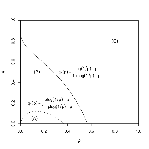
and is thus satisfied for p≤p∗​(q)p\leq p_{*}(q), where p∗​(q)p_{*}(q) is the unique solution of (2.19) in [0,1][0,1]. As in [12] and [16], p∗​(0)≈0.5671p_{*}(0)\approx 0.5671 is the solution to p​ep=1pe^{p}=1; p∗p_{*} is a decreasing function, and p∗​(1)=0p_{*}(1)=0.

In [16], conditions are given as to which moments of the degree weighted process are finite. Here, we use similar arguments to make comparable statements about the moments of X∗X^{*}, when it is positive recurrent. For any u>1u>1, let x∗​(u)x^{*}(u) denote the positive solution to the equation x=u⁡(1−e−x)x=u(1-e^{-x}); note that x∗​(u)<ux^{*}(u)<u.

Theorem 2.4

If α<β​log⁡(1/p)\alpha<\beta\log(1/p), the process X∗X^{*} has a stationary distribution, whose η\eta-th moment is finite for all η<η∗:=x∗​(β​log⁡(1/p)/α)/log⁡(1/p)\eta<\eta^{*}:=x^{*}(\beta\log(1/p)/\alpha)/\log(1/p), and is infinite for all η>η∗\eta>\eta^{*}. In particular, η∗<β/α\eta^{*}<\beta/\alpha.

Proof: If α<β​log⁡(1/p)\alpha<\beta\log(1/p), η≤1\eta\leq 1 and α​η<β⁡(1−pη)\alpha\eta<\beta(1-p^{\eta}), the existence of an η\eta-th moment of the stationary distribution of X∗X^{*} follows from the proof of case (1) in Theorem 2.3, by [18, Theorem 4.2]. If η>1\eta>1 and α​η<β⁡(1−pη)\alpha\eta<\beta(1-p^{\eta}), the inequality (2.8) cannot be established as before, because f⁡(j):=(j+1)ηf(j):=(j+1)^{\eta} is no longer concave. However, as for (2.18), we can use the bound (2.16), valid for this choice of ff for |y−x|≤c⁡(η)​x|y-x|\leq c(\eta)x and for all xx large enough, for some c⁡(η)>0c(\eta)>0. Using Chebyshev’s inequality to bound any contribution from |Yj−j​pj|>c⁡(η)​j​pj|Y_{j}-jp_{j}|>c(\eta)jp_{j}, taking expectations in (2.16) results in the bound

𝔼⁡{f⁡(Yj)}−f⁡(j)≤f⁡(𝔼​Yj)−f⁡(j)+O⁡(jη−γ)=(j+1)η​(pη−1+O⁡(j−γ)),{\mathbb{E}}\{f(Y_{j})\}-f(j)\ \leq\ f({\mathbb{E}}Y_{j})-f(j)+O(j^{\eta-\gamma})\ =\ (j+1)^{\eta}(p^{\eta}-1+O(j^{-\gamma})),

which is the final inequality in (2.8) once again. The remainder of the argument is as before. Note that, if η<η∗\eta<\eta^{*}, then α​η<β⁡(1−pη)\alpha\eta<\beta(1-p^{\eta}).

For η>η∗\eta>\eta^{*}, so that α​η>β⁡(1−pη)\alpha\eta>\beta(1-p^{\eta}), entirely similar arguments can be used to show that

(Q​f)​(j)=f⁡(j)​{α​η+β⁡(pη−1)+O⁡(j−γ)},(Qf)(j)\ =\ f(j)\{\alpha\eta+\beta(p^{\eta}-1)+O(j^{-\gamma})\},

and hence that

(Q​f)​(j)≥cη′​f​(j),where​cη′:=12​{α​η−β⁡(1−pη)}> 0,(Qf)(j)\ \geq\ c^{\prime}_{\eta}f(j),\quad\mbox{where}\ c^{\prime}_{\eta}\ :=\ {\textstyle{\frac{1}{2}}}\{\alpha\eta-\beta(1-p^{\eta})\}\ >\ 0,

for all j≥j0j\geq j_{0}, for some j0j_{0} large enough. Defining f0​(j):=max⁡{f⁡(j0),f⁡(j)}f_{0}(j):=\max\{f(j_{0}),f(j)\}, it thus follows that

(Qf0)(j)≥cη′f0(j),j≥j0;(Qf0)(j)≥ 0,otherwise.(Qf_{0})(j)\ \geq\ c^{\prime}_{\eta}f_{0}(j),\quad j\geq j_{0};\qquad(Qf_{0})(j)\ \geq\ 0,\quad\mbox{otherwise}.

Now, with f⁡(j):=(j+1)ηf(j):=(j+1)^{\eta}, the conditions of [11, Theorem 2] are satisfied by f0f_{0}, implying that f0​(Xt∗)−∫t0t(Q​f0)​(Xs∗)​𝑑sf_{0}(X^{*}_{t})-\int_{t_{0}}^{t}(Qf_{0})(X^{*}_{s})\,ds is a martingale in t≥t0t\geq t_{0}, for any t0t_{0}. If 𝔼​f0​(Xt0∗)<∞{\mathbb{E}}f_{0}(X^{*}_{t_{0}})<\infty, this in turn implies that 𝔼​f0​(Xt∗){\mathbb{E}}f_{0}(X^{*}_{t}) is non-decreasing in t≥t0t\geq t_{0}, and that 𝔼​f0​(Xt∗)>𝔼​f0​(Xt0∗){\mathbb{E}}f_{0}(X^{*}_{t})>{\mathbb{E}}f_{0}(X^{*}_{t_{0}}) for t>t0t>t_{0} if, with positive probability, Xs∗≥j0X^{*}_{s}\geq j_{0} on a subset of [t0,t][t_{0},t] of positive Lebesgue measure; and this is the case if ℙ[Xt0∗≥j0]>0{\mathbb{P}}[X^{*}_{t_{0}}\geq j_{0}]>0, because X∗X^{*} is a pure jump Markov process. Now the stationary distribution of X∗X^{*} assigns positive probability to all states, so that this condition is satisfied if Xt0∗X^{*}_{t_{0}} has the stationary distribution, in which case Xt∗X^{*}_{t} also has the stationary distribution, and 𝔼​f0​(Xt∗)=𝔼​f0​(Xt0∗){\mathbb{E}}f_{0}(X^{*}_{t})={\mathbb{E}}f_{0}(X^{*}_{t_{0}}) if either one is finite. Thus 𝔼​f0​(Xt0∗)<∞{\mathbb{E}}f_{0}(X^{*}_{t_{0}})<\infty is not possible, and the η\eta-th moment of the stationary distribution of X∗X^{*} is infinite.  

3 The path to infinity; almost sure convergence

In view of Theorem 2.3, the event 𝒳{\mathcal{X}}, on which Xt→∞X_{t}\to\infty, has positive probability if α>β​log⁡(1/p)\alpha>\beta\log(1/p). We now investigate how XtX_{t} approaches infinity, when it does so. If βk\beta_{k} took the value zero for all kk, and if αk=α\alpha_{k}=\alpha were the same for all kk, then the process XX would be a Yule process with per capita birth rate α\alpha. In this case, e−α​t​Xte^{-\alpha t}X_{t} would converge almost surely to a positive limit WW. The presence of catastrophes, when β>0\beta>0, changes the behaviour of XX substantially. Nonetheless, there is an analogous almost sure convergence theorem for the bivariate process (X,Z)(X,Z), which, for constant α\alpha and β\beta and binomial thinning, would be a consequence of [17, Theorem 4.1] and [7, Theorem 4.1]. The theorem shows that, on {limt→∞Xt=∞}\{{\lim_{t\to\infty}}X_{t}=\infty\}, XtX_{t} behaves like eα​t​pZt′​We^{\alpha t}p^{Z^{\prime}_{t}}W, where WW is a positive random variable and Z′Z^{\prime} is a Poisson process of rate β\beta. Throughout the section, we assume that

ν:=α−β​log⁡(1/p)> 0;\nu\ :=\ \alpha-\beta\log(1/p)\ >\ 0; (3.1)

for the basic process, ν=α−(1−q)​log⁡(1/p)\nu=\alpha-(1-q)\log(1/p).

Theorem 3.1

If ν>0\nu>0, then Wt:=e−α​t​p−Zt​XtW_{t}:=e^{-\alpha t}p^{-Z_{t}}X_{t} has an almost sure limit as t→∞t\to\infty, which we denote by WW. Furthermore, 𝒳={W>0}{\mathcal{X}}=\{W>0\} almost surely.

The process (Wt,t≥0)(W_{t},\,t\geq 0) is the counterpart, in the process with catastrophes, of the usual non-negative martingale appearing in the Markov branching process, though, in our setting, it is only approximately a martingale. Just as for branching processes, the random variable WW is essentially determined by the early fluctuations of the process. It is easier to understand the behaviour by writing the convergence in the form

log⁡Xt−α​t≈−Zt​log⁡(1/p)+log⁡Ws,\log X_{t}-\alpha t\ \approx\ -Z_{t}\log(1/p)+\log W_{s}, (3.2)

for ss and tt large, but s≪ts\ll t. This is an approximation only because log⁡Ws\log W_{s} is not exactly equal to log⁡Wt\log W_{t}, but the two are close, for ss and tt large, if W>0W>0. Thus the process log⁡Xt−α​t\log X_{t}-\alpha t, instead of being asymptotically constant on {Xt→∞}\{X_{t}\to\infty\}, as in the case of the Yule process, has downward jumps of magnitude log⁡(1/p)\log(1/p), approximately according to a Poisson process of rate β\beta, staying very close to the lattice log⁡W+log⁡(1/p)​ℤ\log W+\log(1/p){\mathbb{Z}}. The origin of the lattice is essentially determined by WsW_{s}, and the development after ss is approximately given by

(log⁡Xt−α​t)−(log⁡Xs−α​s)≈−(Zt−Zs)​log⁡(1/p),(\log X_{t}-\alpha t)-(\log X_{s}-\alpha s)\ \approx\ -(Z_{t}-Z_{s})\log(1/p), (3.3)

where Zt−ZsZ_{t}-Z_{s} is close to a Poisson process of rate β\beta that is independent of XsX_{s}.

The proofs of the counterparts of Theorem 3.1 in [17, Theorem 4.1] and [7, Theorem 4.1] use the fact that, under their assumptions, there is a Galton–Watson process with random environments embedded in the process, enabling techniques from branching processes to be invoked. In our setting, this is no longer the case. Instead, we proceed in a succession of intermediate steps, establishing that log⁡Xt\log X_{t} develops in almost deterministically linear fashion between catastrophes, provided that XtX_{t} is large enough. This is already close to (3.2). The remainder of the argument consists of tidying up the details.

We begin by considering the bivariate process (X,Z)(X,Z) starting a time t0t_{0} in an arbitrary state (j0,k0)(j_{0},k_{0}). Define

T0:=t0;Tn:=inf{t>t0:Zt=k0+n},T_{0}\ :=\ t_{0};\qquad T_{n}\ :=\ \inf\{t>t_{0}\colon\,Z_{t}=k_{0}+n\}, (3.4)

so that TnT_{n} is the time at which ZZ makes its nn-th jump after t0t_{0}. Define X[i]:=XTiX_{[i]}:=X_{T_{i}}. With γ\gamma as in (2.4), and for i≥1i\geq 1, define the following events:

Ai:=Ai(j0,t0):={supTi−1≤t<Ti|logXt−α(t−Ti−1)−logXTi−1|≤XTi−1−γ/4};\displaystyle A_{i}\ :=\ A_{i}(j_{0},t_{0})\ :=\ \Bigl\{\sup_{T_{i-1}\leq t<T_{i}}\Bigl|\log X_{t}-\alpha(t-T_{i-1})-\log X_{T_{i-1}}\Bigr|\leq X_{T_{i-1}}^{-\gamma/4}\Bigr\};
Bi:=Bi(j0,t0):={|logXTi−logp−logXTi−|≤XTi−−γ/4}.\displaystyle B_{i}\ :=\ B_{i}(j_{0},t_{0})\ :=\ \{|\log X_{T_{i}}-\log p-\log X_{T_{i}-}|\leq X_{T_{i}-}^{-\gamma/4}\}. (3.5)

We begin by showing that the events AiA_{i} and BiB_{i} typically hold, if X[i−1]X_{[i-1]} is large, as is eventually the case if Xt→∞X_{t}\to\infty.

Lemma 3.2

With γ\gamma as in (2.4), and for i≥1i\geq 1, the conditional probabilities of AiA_{i} and BiB_{i} can be bounded as follows:

(1):ℙ[Ai(j0,t0)|ℱTi−1]≤CAX[i−1]γ/2−1≤CAX[i−1]−γ/2;\displaystyle(1):\quad{\mathbb{P}}[A_{i}(j_{0},t_{0})\,|\,\mathcal{F}_{T_{i-1}}]\ \leq\ C_{A}X_{[i-1]}^{\gamma/2-1}\ \leq\ C_{A}X_{[i-1]}^{-\gamma/2};
(2):ℙ[Bi(j0,t0)|σ(Ti∨ℱTi−)]≤CBX[i−1]−γ/2.\displaystyle(2):\quad{\mathbb{P}}[B_{i}(j_{0},t_{0})\,|\,\sigma(T_{i}\vee\mathcal{F}_{T_{i}-})]\ \leq\ C_{B}X_{[i-1]}^{-\gamma/2}.

Here, CAC_{A} and CBC_{B} are (finite) constants depending only the sequences (αj,pj,σj2,j≥1)(\alpha_{j},p_{j},\sigma^{2}_{j},\,j\geq 1).

Proof: From time Ti−1T_{i-1} to time TiT_{i}, XX evolves as a pure birth process, with jump rate j​αjj\alpha_{j} when in state jj. Define Yt(i)=XtY^{(i)}_{t}=X_{t} for Ti−1≤t<TiT_{i-1}\leq t<T_{i}, set YTi(i):=YTi−(i)Y^{(i)}_{T_{i}}:=Y^{(i)}_{T_{i}-}, and continue Yt(i)Y^{(i)}_{t} for t>Tit>T_{i} as a pure birth process with the same distribution, independently of the further evolution of XX. With S0:=Ti−1S_{0}:=T_{i-1}, let SlS_{l} be the time of the ll-th jump of Y(i)Y^{(i)}, and let

h⁡(0):= 0;h⁡(j):=∑l=1j1l,j≥1,h(0)\ :=\ 0;\qquad h(j)\ :=\ \sum_{l=1}^{j}\frac{1}{l},\qquad j\geq 1, (3.6)

denote the harmonic numbers. Then, conditional on ℱTi−1∩{X[i−1]=j}\mathcal{F}_{T_{i-1}}\cap\{X_{[i-1]}=j\}, it follows that

Ml:=h⁡(j+l−1)−h⁡(j−1)−∑k=1lαj+k−1​(Sk−Sk−1),l∈ℕ0,M_{l}\ :=\ h(j+l-1)-h(j-1)-\sum_{k=1}^{l}\alpha_{j+k-1}(S_{k}-S_{k-1}),\qquad l\in{\mathbb{N}}_{0}, (3.7)

can be written as the sum ∑k=1lEk′\sum_{k=1}^{l}E^{\prime}_{k}, where

Ek′:=(j+k−1)−1​(1−Ek),E^{\prime}_{k}\ :=\ (j+k-1)^{-1}(1-E_{k}),

and (Ek,k∈ℕ)(E_{k},\,k\in{\mathbb{N}}) are independent standard exponential random variables. Note also that MM can be written in the form

Ml=h⁡(YSl(i)−1)−h⁡(YTi−1(i)−1)−∫Ti−1SlαYu(i)​𝑑u,M_{l}\ =\ h(Y^{(i)}_{S_{l}}-1)-h(Y^{(i)}_{T_{i-1}}-1)-\int_{T_{i-1}}^{S_{l}}\alpha_{Y^{(i)}_{u}}\,du\,, (3.8)

linking the development of the process h⁡(Yt(i))h(Y^{(i)}_{t}) with time, since, in view of (2.3), the integral is close to α⁡(Sl−Ti−1)\alpha(S_{l}-T_{i-1}) if YTi−1(i)Y^{(i)}_{T_{i-1}} is large. Since Var⁡(Ek′)=(j+k−1)−2{\rm Var\,}(E^{\prime}_{k})=(j+k-1)^{-2}, it follows that, for each l≥1l\geq 1,

Var⁡(Ml|ℱTi−1)=∑k=1lVar⁡(Ek′)≤ 2​X[i−1]−1.{\rm Var\,}(M_{l}\,|\,\mathcal{F}_{T_{i-1}})\ =\ \sum_{k=1}^{l}{\rm Var\,}(E^{\prime}_{k})\ \leq\ 2X_{[i-1]}^{-1}. (3.9)

Hence, for any a>0a>0, by Kolmogorov’s inequality,

ℙ⁡[supl≥0|Ml|>a|ℱTi−1]≤2a2​X[i−1].{\mathbb{P}}[\sup_{l\geq 0}|M_{l}|>a\,|\,\mathcal{F}_{T_{i-1}}]\ \leq\ \frac{2}{a^{2}X_{[i-1]}}\,. (3.10)

This inequality controls the fluctuations of (h⁡(YSl(i)−1)−h⁡(YTi−1(i)−1),l≥1)(h(Y^{(i)}_{S_{l}}-1)-h(Y^{(i)}_{T_{i-1}}-1),\,l\geq 1) around the values defined by the integrals (∫Ti−1SlαYu(i)​𝑑u,l≥1)(\int_{T_{i-1}}^{S_{l}}\alpha_{Y^{(i)}_{u}}\,du,\,l\geq 1).

The next step is to bound the differences

Δl:=∫Ti−1SlαYu(i)​𝑑u−α⁡(Sl−Ti−1),l≥1.\Delta_{l}\ :=\ \int_{T_{i-1}}^{S_{l}}\alpha_{Y^{(i)}_{u}}\,du-\alpha(S_{l}-T_{i-1}),\qquad l\geq 1.

We have, for any l≥1l\geq 1,

|𝔼⁡{Δl|ℱTi−1}|\displaystyle|{\mathbb{E}}\{\Delta_{l}\,|\,\mathcal{F}_{T_{i-1}}\}| =\displaystyle= |∑j=X[i−1]X[i−1]+l−1j−1​(1−α/αj)|≤C1​(Δ)​X[i−1]−γ;\displaystyle\biggl|\sum_{j=X_{[i-1]}}^{X_{[i-1]}+l-1}j^{-1}(1-\alpha/\alpha_{j})\biggr|\ \leq\ C_{1}(\Delta)X_{[i-1]}^{-\gamma};
Var⁡(Δl|ℱTi−1)\displaystyle{\rm Var\,}(\Delta_{l}\,|\,\mathcal{F}_{T_{i-1}}) =\displaystyle= ∑j=X[i−1]X[i−1]+l−1j−2​(1−α/αj)2=O⁡(X[i−1]−1−2​γ),\displaystyle\sum_{j=X_{[i-1]}}^{X_{[i-1]}+l-1}j^{-2}(1-\alpha/\alpha_{j})^{2}\ =\ O(X_{[i-1]}^{-1-2\gamma}), (3.11)

from which it also follows, using Kolmogorov’s inequality, that

ℙ⁡[supl≥0|Δl−𝔼​Δl|>a|ℱTi−1]≤C2​(Δ)a2​X[i−1]1+2​γ,{\mathbb{P}}\bigl[\sup_{l\geq 0}|\Delta_{l}-{\mathbb{E}}\Delta_{l}|>a\,|\,\mathcal{F}_{T_{i-1}}\bigr]\ \leq\ \frac{C_{2}(\Delta)}{a^{2}X_{[i-1]}^{1+2\gamma}}\,, (3.12)

for any a>0a>0, where Cl​(Δ)C_{l}(\Delta), l=1,2l=1,2, are constants depending on (αj,j≥1)(\alpha_{j},\,j\geq 1). Hence, for any a>2​C1​(Δ)​XTi−1−γa>2C_{1}(\Delta)X_{T_{i-1}}^{-\gamma},

ℙ⁡[supl≥0|∫Ti−1SlαYu(i)​𝑑u−α⁡(Sl−Ti−1)|>a|ℱTi−1]≤4​C2​(Δ)a2​X[i−1]1+2​γ.{\mathbb{P}}\biggl[\sup_{l\geq 0}\Bigl|\int_{T_{i-1}}^{S_{l}}\alpha_{Y^{(i)}_{u}}\,du-\alpha(S_{l}-T_{i-1})\Bigr|>a\,|\,\mathcal{F}_{T_{i-1}}\biggr]\ \leq\ \frac{4C_{2}(\Delta)}{a^{2}X_{[i-1]}^{1+2\gamma}}\,. (3.13)

In order to recover a bound for the probability of the event AiA_{i} from (3.10) and (3.13), we first observe that, by a simple integral comparison, for l>kl>k, we have

h⁡(l)−h⁡(k)≤∫klx−1​𝑑x=log⁡l−log⁡k≤h⁡(l−1)−h⁡(k−1),h(l)-h(k)\ \leq\ \int_{k}^{l}x^{-1}\,dx\ =\ \log l-\log k\ \leq\ h(l-1)-h(k-1),

implying that |(h⁡(l−1)−h⁡(k−1))−(log⁡l−log⁡k)|≤k−1|(h(l-1)-h(k-1))-(\log l-\log k)|\leq k^{-1}. Then, because Y(i)Y^{(i)} is a step function,

supTi−1≤t≤Sl|h⁡(Yt(i)−1)−h⁡(YTi−1(i)−1)−α⁡(t−Ti−1)|\sup_{T_{i-1}\leq t\leq S_{l}}|h(Y^{(i)}_{t}-1)-h(Y^{(i)}_{T_{i-1}}-1)-\alpha(t-T_{i-1})|

is attained at one of the points {Sk−,Sk, 1≤k≤l}\{S_{k}-,S_{k},\,1\leq k\leq l\}, and |h⁡(YSk(i))−h⁡(YSk−(i))|≤X[i−1]−1|h(Y^{(i)}_{S_{k}})-h(Y^{(i)}_{S_{k}-})|\leq X_{[i-1]}^{-1}. Hence

supt≥t0|log⁡(Yt(i))−log⁡(X[i−1])−α⁡(t−Ti−1)|≤supl≥0|Ml+Δl|+2​X[i−1]−1.\sup_{t\geq t_{0}}|\log(Y^{(i)}_{t})-\log(X_{[i-1]})-\alpha(t-T_{i-1})|\ \leq\ \sup_{l\geq 0}|M_{l}+\Delta_{l}|+2X_{[i-1]}^{-1}. (3.14)

Combining (3.10), (3.13) and (3.14), and because Xt=Yt(i)X_{t}=Y^{(i)}_{t} for Ti−1≤t<TiT_{i-1}\leq t<T_{i}, it follows that, if X[i−1]≥y0X_{[i-1]}\geq y_{0}, where y03​γ/4:=6​max⁡{C1​(Δ),1}y_{0}^{3\gamma/4}:=6\max\{C_{1}(\Delta),1\}, then

ℙ⁡[Aic|ℱTi−1]≤2+4​C2​(Δ)X[i−1]1−γ/2.{\mathbb{P}}[A_{i}^{c}\,|\,\mathcal{F}_{T_{i-1}}]\ \leq\ \frac{2+4C_{2}(\Delta)}{X_{[i-1]}^{1-\gamma/2}}\,.

This establishes the first inequality, with CA:=max⁡{2+4​C2​(Δ),x01−γ/2}C_{A}:=\max\{2+4C_{2}(\Delta),x_{0}^{1-\gamma/2}\}.

The inequality (2) is much easier. We first note that

ℙ[Bic|σ(Ti∨ℱTi−)∩{XTi−=j}]=ℙ[|logYj−logp−logj|>j−γ/4],{\mathbb{P}}[B_{i}^{c}\,|\,\sigma(T_{i}\vee\mathcal{F}_{T_{i}-})\cap\{X_{T_{i}-}=j\}]\ =\ {\mathbb{P}}[|\log Y_{j}-\log p-\log j|>j^{-\gamma/4}],

where Yj∼ΠjY_{j}\sim\Pi_{j}, as before. Now, by (1.1),

ℙ[|logYj−logp−logj|>j−γ/4]≤ℙ[|logYj−logpj−logj|>12j−γ/4]{\mathbb{P}}[|\log Y_{j}-\log p-\log j|>j^{-\gamma/4}]\ \leq\ {\mathbb{P}}[|\log Y_{j}-\log p_{j}-\log j|>{\textstyle{\frac{1}{2}}}j^{-\gamma/4}]

if 12j−γ/4>c2j−γ{\textstyle{\frac{1}{2}}}j^{-\gamma/4}>c_{2}j^{-\gamma}, and, since |log⁡(1+x)|≤2​|x||\log(1+x)|\leq 2|x| in x≥−1/2x\geq-1/2,

ℙ[|logYj−logpj−logj|>12j−γ/4]≤ℙ[|(Yj/jpj)−1|>14j−γ/4]≤4​c3pj2j−γ/2,{\mathbb{P}}[|\log Y_{j}-\log p_{j}-\log j|>{\textstyle{\frac{1}{2}}}j^{-\gamma/4}]\ \leq\ {\mathbb{P}}[|(Y_{j}/jp_{j})-1|>{\textstyle{\frac{1}{4}}}j^{-\gamma/4}]\ \leq\ \frac{4c_{3}}{p_{j}^{2}}\,j^{-\gamma/2},

where the last inequality follows by Chebyshev’s inequality, and because of (1.1). Inequality (2) now follows directly.  

The implication of Lemma 3.2 is that, if X[i−1]X_{[i-1]} is large, then Ai∩BiA_{i}\cap B_{i} occurs with high probability, in which case log⁡Xt\log X_{t} stays close to α⁡(t−Ti−1)+log⁡X[i−1]\alpha(t-T_{i-1})+\log X_{[i-1]} for Ti−1≤t<TiT_{i-1}\leq t<T_{i}, and log⁡X[i]\log X_{[i]} is close to α⁡(Ti−Ti−1)+log⁡X[i−1]−log⁡(1/p)\alpha(T_{i}-T_{i-1})+\log X_{[i-1]}-\log(1/p). If this is the case for all 1≤j≤i1\leq j\leq i, then log⁡Xt\log X_{t} stays close to α⁡(t−T0)−(Zt−ZT0)​log⁡(1/p)+log⁡X[0]\alpha(t-T_{0})-(Z_{t}-Z_{T_{0}})\log(1/p)+\log X_{[0]} for 0≤t≤Ti0\leq t\leq T_{i}. Now 𝔼⁡{Zt−ZT0}≈β⁡(t−T0){\mathbb{E}}\{Z_{t}-Z_{T_{0}}\}\approx\beta(t-T_{0}), and so α⁡(t−T0)−𝔼⁡{Zt−ZT0}​log⁡(1/p)≈ν⁡(t−T0)\alpha(t-T_{0})-{\mathbb{E}}\{Z_{t}-Z_{T_{0}}\}\log(1/p)\approx\nu(t-T_{0}), where ν\nu is as in (3.1). If ν>0\nu>0, this suggests that log⁡Xt\log X_{t} grows linearly with tt, or, equivalently, that XtX_{t} grows exponentially with tt, on the event

H:=H⁡(j0,t0):=⋂i≥1{Ai​(j0,t0)∩Bi​(j0,t0)}.H\ :=\ H(j_{0},t_{0}):=\bigcap_{i\geq 1}\bigl\{A_{i}(j_{0},t_{0})\cap B_{i}(j_{0},t_{0})\bigr\}.

The remainder of the proof consists of making this heuristic precise.

We begin by investigating the times TjT_{j} defined in (3.4), again for the process (X,Z)(X,Z) starting a time t0t_{0} in an arbitrary state (j0,k0)(j_{0},k_{0}). Let j′j^{\prime} be such that, for all j≥j′j\geq j^{\prime},

α−βj​log⁡(1/p)>ν/2> 0;\alpha-\beta_{j}\log(1/p)\ >\ \nu/2\ >\ 0; (3.15)

write β′:=supk≥j′βk\beta^{\prime}:=\sup_{k\geq j^{\prime}}\beta_{k}. Observe that the process (Tj,j≥1)(T_{j},\,j\geq 1) is a point process adapted to the filtration (ℱt,t≥t0)(\mathcal{F}_{t},\,t\geq t_{0}), with compensator A⁡(t):=∫t0tβXu​𝑑uA(t):=\int_{t_{0}}^{t}\beta_{X_{u}}\,du. Hence, as long as Xu≥j′X_{u}\geq j^{\prime} for all uu, it can be coupled to a point process (Tj′,j≥1)(T^{\prime}_{j},\,j\geq 1) with compensator A′​(t):=β′​(t−t0)A^{\prime}(t):=\beta^{\prime}(t-t_{0}), hence a Poisson process with rate β′\beta^{\prime}, in such a way that Tj−Tj−1≥Tj′−Tj−1′T_{j}-T_{j-1}\geq T^{\prime}_{j}-T^{\prime}_{j-1} a.s. for all j≥1j\geq 1, where we take T0:=T0′:=t0T_{0}:=T_{0}^{\prime}:=t_{0}. More precisely, taking a sequence (Uj,j≥1)(U_{j},\,j\geq 1) of independent uniform U⁡[0,1]\mathrm{U}[0,1] random variables, independent of everything else, define

Tj′−Tj−1′\displaystyle T^{\prime}_{j}-T^{\prime}_{j-1} :⁣=\displaystyle:= −1β′​log⁡Uj=inf{t≥0:β′​t≥−log⁡Uj};\displaystyle-\frac{1}{\beta^{\prime}}\log U_{j}\ =\ \inf\{t\geq 0\colon\beta^{\prime}t\geq-\log U_{j}\};
Tj−Tj−1\displaystyle T_{j}-T_{j-1} :⁣=\displaystyle:= inf{t≥0:∫Tj−1tβXu​𝑑u≥−log⁡Uj},\displaystyle\inf\Bigl\{t\geq 0\colon\int_{T_{j-1}}^{t}\beta_{X_{u}}\,du\geq-\log U_{j}\Bigr\}, (3.16)

so that the times of the ZZ-jumps in (X,Z)(X,Z) are defined in terms of the sequence (Uj,j≥1)(U_{j},\,j\geq 1); the times of the remaining transitions in (X,Z)(X,Z) are defined using an independent sequence (Uj′,j≥1)(U^{\prime}_{j},\,j\geq 1) of uniform random variables. On the event X[j−1]≥j′X_{[j-1]}\geq j^{\prime}, we then have Tj−Tj−1≥Tj′−Tj−1′T_{j}-T_{j-1}\geq T^{\prime}_{j}-T^{\prime}_{j-1}, since XX is non-decreasing in [Tj−1,Tj)[T_{j-1},T_{j}) .

For any η>0\eta>0 and with γ\gamma as in (2.4), define the events

ℰiη\displaystyle\mathcal{E}_{i}^{\eta} :=ℰiη(j0,t0):={min1≤j≤i{α(Tj′−t0)−j(log(1/p)+η)+logj0}>(4/γ)log(2/η)};\displaystyle\ :=\ \mathcal{E}_{i}^{\eta}(j_{0},t_{0})\ :=\ \Bigl\{\min_{1\leq j\leq i}\{\alpha(T_{j}^{\prime}-t_{0})-j(\log(1/p)+\eta)+\log j_{0}\}>(4/\gamma)\log(2/\eta)\Bigr\};
Hi\displaystyle H_{i} :=Hi​(j0,t0):=⋂j=1i(Aj​(j0,t0)∩Bj​(j0,t0)).\displaystyle\ :=\ H_{i}(j_{0},t_{0})\ :=\ \bigcap_{j=1}^{i}\bigl(A_{j}(j_{0},t_{0})\cap B_{j}(j_{0},t_{0})\bigr). (3.17)

The next step is to show that, on the event ℰiη​(j0,t0)∩Hi​(j0,t0)\mathcal{E}_{i}^{\eta}(j_{0},t_{0})\cap H_{i}(j_{0},t_{0}), the values of X[i]=XTiX_{[i]}=X_{T_{i}} can be bounded below in terms of the times Ti′T^{\prime}_{i}.

Lemma 3.3

If ν>0\nu>0, choose any η>0\eta>0 such that (2/η)4/γ>j′(2/\eta)^{4/\gamma}>j^{\prime}, where j′j^{\prime} is as defined in (3.15). Then, for any j0>(2/η)4/γj_{0}>(2/\eta)^{4/\gamma}, on the event ℰiη​(j0,t0)∩Hi​(j0,t0)\mathcal{E}_{i}^{\eta}(j_{0},t_{0})\cap H_{i}(j_{0},t_{0}), it follows that

2X[j]−γ/4<ηandlogX[j]≥α(Tj′−t0)−j(log(1/p)+η)+logj02X_{[j]}^{-\gamma/4}\ <\ \eta\quad\mbox{and}\quad\log X_{[j]}\ \geq\ \alpha(T_{j}^{\prime}-t_{0})-j(\log(1/p)+\eta)+\log j_{0} (3.18)

for all 0≤j≤i0\leq j\leq i.

Proof: The proof runs by induction on jj. By assumption, 2X[0]−γ/4=2j0−γ/4<η2X_{[0]}^{-\gamma/4}=2j_{0}^{-\gamma/4}<\eta, and the second inequality is trivial for j=0j=0. If (3.18), with j−1j-1 for jj, is true for some jj, then, from the definitions (3.5) of Aj​(j0,t0)A_{j}(j_{0},t_{0}) and Bj​(j0,t0)B_{j}(j_{0},t_{0}),

log⁡X[j]−log⁡X[j−1]\displaystyle\log X_{[j]}-\log X_{[j-1]}\ ≥α(Tj−Tj−1)−log(1/p)−2X[j−1]−γ/4\displaystyle\geq\ \alpha(T_{j}-T_{j-1})-\log(1/p)-2X_{[j-1]}^{-\gamma/4}
≥α⁡(Tj′−Tj−1′)−(log⁡(1/p)+η);\displaystyle\geq\ \alpha(T_{j}^{\prime}-T_{j-1}^{\prime})-(\log(1/p)+\eta);

here, we have used 2X[j−1]−γ/4<η2X_{[j-1]}^{-\gamma/4}<\eta, so that X[j−1]≥j′X_{[j-1]}\geq j^{\prime}; and then also the fact that XX is non-decreasing on [Tj−1,Tj)[T_{j-1},T_{j}), so that βXu≤β′\beta_{X_{u}}\leq\beta^{\prime} for all Tj−1≤u<TjT_{j-1}\leq u<T_{j}. Adding this inequality to the second induction hypothesis gives

log⁡X[j]≥α⁡(Tj′−t0)−j⁡(log⁡(1/p)+η)+log⁡j0>(4/γ)​log⁡(2/η),\log X_{[j]}\ \geq\ \alpha(T_{j}^{\prime}-t_{0})-j(\log(1/p)+\eta)+\log j_{0}\ \ >\ (4/\gamma)\log(2/\eta),

in view of ℰiη​(j0,t0)\mathcal{E}_{i}^{\eta}(j_{0},t_{0}), implying that 2X[j]−γ/4<η2X_{[j]}^{-\gamma/4}<\eta also.  

The lower bound established in Lemma 3.3 is useful for establishing that the values X[j]X_{[j]} grow geometrically fast with jj for 1≤j≤i1\leq j\leq i, on the event ℰiη​(j0,t0)∩Hi​(j0,t0)\mathcal{E}_{i}^{\eta}(j_{0},t_{0})\cap H_{i}(j_{0},t_{0}), provided that the distribution of the times (Tj′,j≥1)(T_{j}^{\prime},\,j\geq 1) can be controlled. This is made possible by the next lemma.

Lemma 3.4

Let (Ei,i≥1)(E_{i},\,i\geq 1) be independent standard exponential random variables, and let Vi:=∑j=1iEjV_{i}:=\sum_{j=1}^{i}E_{j}.

(i). For any 0<ϕ<10<\phi<1, let u⁡(ϕ)u(\phi) be the positive solution to u​ϕ=log⁡(1+u)u\phi=\log(1+u). Then, for any a>0a>0,

ℙ[minj≥1{Vj−jϕ}≤−a]≤e−a​u​(ϕ).{\mathbb{P}}[\min_{j\geq 1}\{V_{j}-j\phi\}\leq-a]\ \leq\ e^{-au(\phi)}.

(ii). For any 0<ϕ<10<\phi<1 and c,a>0c,a>0, there exist k=k⁡(ϕ,c)>0k=k(\phi,c)>0 and 0<ψ=ψ⁡(ϕ,c)<10<\psi=\psi(\phi,c)<1 such that

∑i≥i0𝔼⁡{min⁡(1,e−c⁡(Vi−i​ϕ+a))}≤k​ψmax⁡{i0,a},i0≥1.\sum_{i\geq i_{0}}{\mathbb{E}}\bigl\{\min\bigl(1,\,e^{-c(V_{i}-i\phi+a)}\bigr)\bigr\}\ \leq\ k\psi^{\max\{i_{0},a\}},\quad i_{0}\geq 1.

Hence, in particular,

∑i≥1min⁡(1,e−c⁡(Vi−i​ϕ+a))<∞​a.s.\sum_{i\geq 1}\min\bigl(1,\,e^{-c(V_{i}-i\phi+a)}\bigr)\ <\ \infty\ \mbox{a.s.}

Proof: For part (i), it is immediate that the sequence Mju:=e−u​Vj+j​log⁡(1+u)M_{j}^{u}:=e^{-uV_{j}+j\log(1+u)} is a martingale for any u>−1u>-1. Writing σ⁡(a):=inf{j≥0:Vj−j​ϕ≤−a}\sigma(a):=\inf\{j\geq 0\colon V_{j}-j\phi\leq-a\}, it thus follows that, for any n≥1n\geq 1,

1\displaystyle 1 =\displaystyle= 𝔼{Mσ⁡(a)∧nu⁡(ϕ)}=𝔼{e−u⁡(ϕ)​(Vσ⁡(a)∧n−(σ⁡(a)∧n)​ϕ)}≥ℙ[σ(a)≤n]ea​u​(ϕ),\displaystyle{\mathbb{E}}\{M^{u(\phi)}_{\sigma(a)\wedge n}\}\ =\ {\mathbb{E}}\bigl\{e^{-u(\phi)(V_{\sigma(a)\wedge n}-(\sigma(a)\wedge n)\phi)}\bigr\}\ \geq\ {\mathbb{P}}[\sigma(a)\leq n]e^{au(\phi)},

from which part (i) follows.

For part (ii), observe first that, for any ϕ′∈(ϕ,1)\phi^{\prime}\in(\phi,1), we have

𝔼⁡{min⁡(1,e−c⁡(Vi−i​ϕ+a))}\displaystyle{\mathbb{E}}\bigl\{\min\bigl(1,\,e^{-c(V_{i}-i\phi+a)}\bigr)\bigr\} ≤\displaystyle\leq ℙ[Vi≤iϕ′−a/2]+𝔼{e−c⁡(Vi−i​ϕ+a)I[Vi>iϕ′−a/2]}\displaystyle{\mathbb{P}}[V_{i}\leq i\phi^{\prime}-a/2]+{\mathbb{E}}\bigl\{e^{-c(V_{i}-i\phi+a)}I[V_{i}>i\phi^{\prime}-a/2]\bigr\} (3.19)
≤\displaystyle\leq ℙ[Vi≤iϕ′−a/2]+e−c​i​(ϕ′−ϕ)−c​a/2.\displaystyle{\mathbb{P}}[V_{i}\leq i\phi^{\prime}-a/2]+e^{-ci(\phi^{\prime}-\phi)-ca/2}.

If i​ϕ′≤a/2i\phi^{\prime}\leq a/2, ℙ[Vi≤iϕ′−a/2]=0{\mathbb{P}}[V_{i}\leq i\phi^{\prime}-a/2]=0. For i​ϕ′>a/2i\phi^{\prime}>a/2, take u2​(ϕ′):=12​u​(ϕ′)u_{2}(\phi^{\prime}):={\textstyle{\frac{1}{2}}}u(\phi^{\prime}), for which

v⁡(ϕ′):=log⁡(1+u2​(ϕ′))−ϕ′​u2​(ϕ′)> 0,v(\phi^{\prime})\ :=\ \log(1+u_{2}(\phi^{\prime}))-\phi^{\prime}u_{2}(\phi^{\prime})\ >\ 0,

beacuse the function log⁡(1+u)\log(1+u) is strictly concave, and log⁡(1+u)=u​ϕ′\log(1+u)=u\phi^{\prime} for u=0u=0 and u⁡(ϕ′)u(\phi^{\prime}). Then

1\displaystyle 1 =\displaystyle= 𝔼{Miu2​(ϕ′)}≥𝔼{exp{−u2(ϕ′)Vi+ilog(1+u2(ϕ′))}I[Vi≤iϕ′−a/2]}\displaystyle{\mathbb{E}}\{M_{i}^{u_{2}(\phi^{\prime})}\}\ \geq\ {\mathbb{E}}\bigl\{\exp\{-u_{2}(\phi^{\prime})V_{i}+i\log(1+u_{2}(\phi^{\prime}))\}I[V_{i}\leq i\phi^{\prime}-a/2]\bigr\}
≥\displaystyle\geq ea​u2​(ϕ′)/2+i​v​(ϕ′)ℙ[Vi≤iϕ′−a/2].\displaystyle e^{au_{2}(\phi^{\prime})/2+iv(\phi^{\prime})}{\mathbb{P}}[V_{i}\leq i\phi^{\prime}-a/2].

Hence

∑i≥i0ℙ[Vi≤iϕ′−a/2]≤e−au2(ϕ′)/2e−i0​v​(ϕ′)1−e−v⁡(ϕ′).\sum_{i\geq i_{0}}{\mathbb{P}}[V_{i}\leq i\phi^{\prime}-a/2]\ \leq\ e^{-au_{2}(\phi^{\prime})/2}\,\frac{e^{-i_{0}v(\phi^{\prime})}}{1-e^{-v(\phi^{\prime})}}\,. (3.20)

Since also

∑i≥i0e−c​i​(ϕ′−ϕ)−c​a/2≤e−ca/2e−i0​c​(ϕ′−ϕ)1−e−c⁡(ϕ′−ϕ),\sum_{i\geq i_{0}}e^{-ci(\phi^{\prime}-\phi)-ca/2}\ \leq\ e^{-ca/2}\,\frac{e^{-i_{0}c(\phi^{\prime}-\phi)}}{1-e^{-c(\phi^{\prime}-\phi)}}\,,

the second part follows from (3.19).  

The next step is to use Lemmas 3.2–3.4 to conclude that, by choosing j0j_{0} large enough, the probability ℙ⁡[H⁡(j0,t0)∩ℰη​(j0,t0)]{\mathbb{P}}[H(j_{0},t_{0})\cap\mathcal{E}^{\eta}(j_{0},t_{0})] can be made arbitrarily close to 11; here, ℰη​(j0,t0):=⋂i≥1ℰiη​(j0,t0)\mathcal{E}^{\eta}(j_{0},t_{0}):=\bigcap_{i\geq 1}\mathcal{E}_{i}^{\eta}(j_{0},t_{0}).

Lemma 3.5

Assume that ν:=α−β​log⁡(1/p)>0\nu:=\alpha-\beta\log(1/p)>0, and choose any 0<θ<10<\theta<1 and η>0\eta>0 such that

η≤θ​ν′β′and(2η)4/γ>j′,\eta\ \leq\ \frac{\theta\nu^{\prime}}{\beta^{\prime}}\quad\mbox{and}\quad\Bigl(\frac{2}{\eta}\Bigr)^{4/\gamma}\ >\ j^{\prime}, (3.21)

where ν′:=α−β′​log⁡(1/p)>0\nu^{\prime}:=\alpha-\beta^{\prime}\log(1/p)>0, and β′\beta^{\prime} and j′j^{\prime} are as in (3.15). Then

ℙ⁡[H⁡(j0,t0)∩ℰη​(j0,t0)]≥ 1−C0​j0−δ0,{\mathbb{P}}[H(j_{0},t_{0})\cap\mathcal{E}^{\eta}(j_{0},t_{0})]\ \geq\ 1-C_{0}j_{0}^{-\delta_{0}},

for 0<δ0,C0<∞0<\delta_{0},C_{0}<\infty depending only on the sequences (αj,βj,pj,σj2)(\alpha_{j},\beta_{j},p_{j},\sigma^{2}_{j}) and θ\theta.

Proof: First, we show that ℙ⁡[(ℰζ​(j0,t0))c]{\mathbb{P}}[(\mathcal{E}^{\zeta}(j_{0},t_{0}))^{c}] is small if j0j_{0} is large, for all ζ≤η\zeta\leq\eta. Writing ϕζ:=β′​(log⁡(1/p)+ζ)/α≤ϕη<1\phi_{\zeta}:=\beta^{\prime}(\log(1/p)+\zeta)/\alpha\leq\phi_{\eta}<1, the process (α⁡(Tj′−t0)−j⁡(log⁡(1/p)+ζ),j≥0)(\alpha(T_{j}^{\prime}-t_{0})-j(\log(1/p)+\zeta),\,j\geq 0) is that of the partial sums of independent random variables (α/β′)​(Ej−ϕζ)(\alpha/\beta^{\prime})(E_{j}-\phi_{\zeta}), where (Ej,j≥1)(E_{j},\,j\geq 1) is a sequence of independent exponential random variables with mean 11. Hence, by Lemma 3.4 (i), for any a>0a>0,

ℙ[Mζ≤−a]≤e−au(ϕζ)β′/α,whereMζ:=minj≥1{α(Tj′−t0)−j(log(1/p)+ζ)}.{\mathbb{P}}[M_{\zeta}\leq-a]\ \leq\ e^{-au(\phi_{\zeta})\beta^{\prime}/\alpha},\quad\mbox{where}\quad M_{\zeta}\ :=\ \min_{j\geq 1}\{\alpha(T_{j}^{\prime}-t_{0})-j(\log(1/p)+\zeta)\}.

Hence

ℙ[(ℰζ(j0,t0))c]=ℙ[Mζ≤(4/γ)log(2/ζ)−logj0]\displaystyle{\mathbb{P}}[(\mathcal{E}^{\zeta}(j_{0},t_{0}))^{c}]\ =\ {\mathbb{P}}[M_{\zeta}\leq(4/\gamma)\log(2/\zeta)-\log j_{0}] ≤{(ζ2)4/γj0}−u(ϕζ)β′/α.\displaystyle\ \leq\ \biggl\{\Bigl(\frac{\zeta}{2}\Bigr)^{4/\gamma}j_{0}\biggr\}^{-u(\phi_{\zeta})\beta^{\prime}/\alpha}. (3.22)

Next, we express ℙ⁡[H​(j0,t0)c∩ℰη​(j0,t0)]{\mathbb{P}}[H(j_{0},t_{0})^{c}\cap\mathcal{E}^{\eta}(j_{0},t_{0})] in the form

ℙ⁡[Hc∩ℰη]\displaystyle{\mathbb{P}}[H^{c}\cap\mathcal{E}^{\eta}] =ℙ⁡[(⋂i≥1Hi)c∩ℰη]\displaystyle\ =\ {\mathbb{P}}\Bigl[\Bigl(\bigcap_{i\geq 1}H_{i}\Bigr)^{c}\cap\mathcal{E}^{\eta}\Bigr]
=ℙ⁡[(A1∩B1)c∩ℰη]+∑i≥1ℙ⁡[Hi∩(Ai+1∩Bi+1)c∩ℰη].\displaystyle\ =\ {\mathbb{P}}[(A_{1}\cap B_{1})^{c}\cap\mathcal{E}^{\eta}]+\sum_{i\geq 1}{\mathbb{P}}[H_{i}\cap(A_{i+1}\cap B_{i+1})^{c}\cap\mathcal{E}^{\eta}]. (3.23)

Now, because ℰη⊂ℰiη\mathcal{E}^{\eta}\subset\mathcal{E}^{\eta}_{i} for each ii, we have

ℙ⁡[Hi∩(Ai+1∩Bi+1)c∩ℰη]\displaystyle{\mathbb{P}}[H_{i}\cap(A_{i+1}\cap B_{i+1})^{c}\cap\mathcal{E}^{\eta}] ≤ℙ⁡[Hi∩(Ai+1∩Bi+1)c∩ℰiη]\displaystyle\ \leq\ {\mathbb{P}}[H_{i}\cap(A_{i+1}\cap B_{i+1})^{c}\cap\mathcal{E}^{\eta}_{i}]
=𝔼⁡{ℙ⁡[Hi∩(Ai+1∩Bi+1)c∩ℰiη|ℱTi]},\displaystyle\ =\ {\mathbb{E}}\{{\mathbb{P}}[H_{i}\cap(A_{i+1}\cap B_{i+1})^{c}\cap\mathcal{E}^{\eta}_{i}\,|\,\mathcal{F}_{T_{i}}]\}, (3.24)

and it is immediate that

ℙ⁡[Hi∩(Ai+1∩Bi+1)c∩ℰiη|ℱTi]\displaystyle{\mathbb{P}}[H_{i}\cap(A_{i+1}\cap B_{i+1})^{c}\cap\mathcal{E}^{\eta}_{i}\,|\,\mathcal{F}_{T_{i}}] =ℙ⁡[(Ai+1∩Bi+1)c|ℱTi]​I​[Hi∩ℰiη].\displaystyle\ =\ {\mathbb{P}}[(A_{i+1}\cap B_{i+1})^{c}\,|\,\mathcal{F}_{T_{i}}]I[H_{i}\cap\mathcal{E}^{\eta}_{i}]. (3.25)

From Lemma 3.2 and both inequalities in Lemma 3.3, it thus follows that

ℙ[Hi\displaystyle{\mathbb{P}}[H_{i} ∩(Ai+1∩Bi+1)c∩ℰiη|ℱTi]≤(CA+CB)X[i]−(γ/2)I[Hi∩ℰiη]\displaystyle\cap(A_{i+1}\cap B_{i+1})^{c}\cap\mathcal{E}^{\eta}_{i}\,|\,\mathcal{F}_{T_{i}}]\ \leq\ (C_{A}+C_{B})X_{[i]}^{-(\gamma/2)}I[H_{i}\cap\mathcal{E}^{\eta}_{i}]
≤(CA+CB)​min​{1,exp⁡{−(γ/2)​(α⁡(Ti′−t0)−i⁡(log⁡(1/p)+η)+log⁡j0)}},\displaystyle\ \leq\ (C_{A}+C_{B})\min\bigl\{1,\exp\{-(\gamma/2)(\alpha(T_{i}^{\prime}-t_{0})-i(\log(1/p)+\eta)+\log j_{0})\}\bigr\}, (3.26)

where we have used j′≥1j^{\prime}\geq 1. Combining (3.24) and (3.26), it follows that

ℙ⁡[Hi∩(Ai+1∩Bi+1)c∩ℰη]\displaystyle{\mathbb{P}}[H_{i}\cap(A_{i+1}\cap B_{i+1})^{c}\cap\mathcal{E}^{\eta}] ≤(CA+CB)​𝔼​{1∧e−c⁡(Vi−i​ϕη+a0)},\displaystyle\ \leq\ (C_{A}+C_{B}){\mathbb{E}}\bigl\{1\wedge e^{-c(V_{i}-i\phi_{\eta}+a_{0})}\Bigr\}, (3.27)

where ViV_{i} and ϕa\phi_{a} are as before,

c:=α​γ2​β′> 0anda0:=β′​log⁡j0α.c\ :=\ \frac{\alpha\gamma}{2\beta^{\prime}}\ >\ 0\quad\mbox{and}\quad a_{0}\ :=\ \frac{\beta^{\prime}\log j_{0}}{\alpha}\,.

Applying Lemma 3.4 (ii), it follows from (3.23) and (3.27) that

ℙ⁡[Hc∩ℰη]≤(CA+CB)​k​(ϕη,c)​{ψ⁡(ϕη,c)}a0;{\mathbb{P}}[H^{c}\cap\mathcal{E}^{\eta}]\ \leq\ (C_{A}+C_{B})k(\phi_{\eta},c)\{\psi(\phi_{\eta},c)\}^{a_{0}}; (3.28)

taking ζ=η\zeta=\eta in (3.22), together with (3.28) and the definition of a0a_{0}, proves the lemma.  

With these preparations, it is now possible to prove Theorem 3.1.

Proof of Theorem 3.1. For any j∈ℕj\in{\mathbb{N}}, let T0=τ⁡(j):=inf{t>0:Xt=j}≤∞T_{0}=\tau(j):=\inf\{t>0\colon X_{t}=j\}\leq\infty. Then, defining 𝒳j:={τ(j)<∞}{\mathcal{X}}_{j}:=\{\tau(j)<\infty\}, we have ℙ⁡[H⁡(j,τ⁡(j))∩ℰη​(j,τ⁡(j))|𝒳j]≥ 1−C0​j−δ0{\mathbb{P}}[H(j,\tau(j))\cap\mathcal{E}^{\eta}(j,\tau(j))\,|\,{\mathcal{X}}_{j}]\ \geq\ 1-C_{0}j^{-\delta_{0}}, by Lemma 3.5 and the strong Markov property. On the event H⁡(j,τ⁡(j))∩ℰη​(j,τ⁡(j))H(j,\tau(j))\cap\mathcal{E}^{\eta}(j,\tau(j)), for any r≥0r\geq 0, we have

supt≥Tr|logXt−α(t−Tr)+(Zt−ZTr)log(1/p)−logX[r]|≤ 2∑l≥rX[l]−γ/4,\sup_{t\geq T_{r}}|\log X_{t}-\alpha(t-T_{r})+(Z_{t}-Z_{T_{r}})\log(1/p)-\log X_{[r]}|\ \leq\ 2\sum_{l\geq r}X_{[l]}^{-\gamma/4}, (3.29)

and hence, recalling that Wt:=e−α​t​p−Zt​XtW_{t}:=e^{-\alpha t}p^{-Z_{t}}X_{t}, it follows that

sups,t≥Tr|logWt−logWs|≤ 4∑l≥rX[l]−γ/4.{\sup_{s,t\geq T_{r}}|\log W_{t}-\log W_{s}|\ \leq\ 4\sum_{l\geq r}X_{[l]}^{-\gamma/4}.} (3.30)

Then, by Lemma 3.3, on the event H⁡(j,τ⁡(j))∩ℰη​(j,τ⁡(j))H(j,\tau(j))\cap\mathcal{E}^{\eta}(j,\tau(j)), we have

X[i]≥max⁡{1,j​eα⁡(Ti′−T0)−i⁡(log⁡(1/p)+η)}for all​i≥0,X_{[i]}\ \geq\ \max\bigl\{1,\,je^{\alpha(T_{i}^{\prime}-T_{0})-i(\log(1/p)+\eta)}\bigr\}\quad\mbox{for all}\ i\geq 0, (3.31)

and this, in turn, from Lemma 3.4, implies that ∑i≥1X[i]−γ/4<∞\sum_{i\geq 1}X_{[i]}^{-\gamma/4}<\infty a.s., and hence that, on the event H⁡(j,τ⁡(j))∩ℰη​(j,τ⁡(j))H(j,\tau(j))\cap\mathcal{E}^{\eta}(j,\tau(j)),

limr→∞∑i≥rX[i]−γ/4= 0a.s.{\lim_{r\to\infty}\sum_{i\geq r}X_{[i]}^{-\gamma/4}\ =\ 0\ \ \mbox{a.s.}} (3.32)

Thus, on the event

A⁡(j):=𝒳j∩H⁡(j,τ⁡(j))∩ℰη​(j,τ⁡(j)),A(j)\ :=\ {\mathcal{X}}_{j}\cap H(j,\tau(j))\cap\mathcal{E}^{\eta}(j,\tau(j)),

we conclude from (3.30) and (3.32), using the Cauchy criterion, that log⁡Wt\log W_{t} converges a.s. to a finite limit, implying that WtW_{t} converges a.s. to a strictly positive limit WW.

Now, for X0=x0X_{0}=x_{0}, 𝒳=⋂j>x0𝒳j{\mathcal{X}}=\bigcap_{j>x_{0}}{\mathcal{X}}_{j}. Writing ℙj​[⋅]{\mathbb{P}}_{j}[\cdot] for ℙ[⋅|X0=j]{\mathbb{P}}[\cdot\,|\,X_{0}=j], this implies that ℙx0​[𝒳]=limj→∞ℙx0​[𝒳j]{\mathbb{P}}_{x_{0}}[{\mathcal{X}}]=\lim_{j\to\infty}{\mathbb{P}}_{x_{0}}[{\mathcal{X}}_{j}], and, as above, A⁡(j)⊂𝒳jA(j)\subset{\mathcal{X}}_{j} and, using Lemma 3.5,

0≤ℙx0​[𝒳j]−ℙx0​[A⁡(j)]≤ℙx0​[𝒳j]​C0​j−δ0→ 0as​j→∞.0\ \leq\ {\mathbb{P}}_{x_{0}}[{\mathcal{X}}_{j}]-{\mathbb{P}}_{x_{0}}[A(j)]\ \leq\ {\mathbb{P}}_{x_{0}}[{\mathcal{X}}_{j}]C_{0}j^{-\delta_{0}}\ \to\ 0\quad\mbox{as}\ j\to\infty.

Hence, if C:={Wt​ converges to a positive limit}C:=\{W_{t}\mbox{ converges to a positive limit}\}, we have A⁡(j)⊂CA(j)\subset C for each jj, and

lim supj→∞ℙx0​[A⁡(j)]=limj→∞ℙx0​[𝒳j]=ℙx0​[𝒳].\limsup_{j\to\infty}{\mathbb{P}}_{x_{0}}[A(j)]\ =\ \lim_{j\to\infty}{\mathbb{P}}_{x_{0}}[{\mathcal{X}}_{j}]\ =\ {\mathbb{P}}_{x_{0}}[{\mathcal{X}}].

Hence ℙx0​[C]≥ℙx0​[𝒳]{\mathbb{P}}_{x_{0}}[C]\geq{\mathbb{P}}_{x_{0}}[{\mathcal{X}}]. However, 𝒳c={Xt=0 eventually}{\mathcal{X}}^{c}=\{X_{t}=0\mbox{ eventually}\}, on which event Wt→0W_{t}\to 0 a.s. Hence C=𝒳C={\mathcal{X}} a.s., and the theorem is proved.  

4 The path to infinity: the central limit theorem

In view of Theorem 3.1, and its interpretation in (3.3), the main fluctuations in log⁡Xt\log X_{t}, for large tt, are governed by those of a Poisson process. In keeping with this interpretation, we now deduce a central limit theorem for log⁡Xt\log X_{t}, which is based on the central limit theorem for the Poisson distribution. As a consequence, for large tt, that part of the distribution of XtX_{t} that is not the mass on zero has an approximately log-normal distribution.

Theorem 4.1

Under the assumptions of Theorem 3.1, for any x0∈ℕx_{0}\in{\mathbb{N}}, the process XX with X0=x0X_{0}=x_{0} satisfies

limt→∞ℙx0[t−1/2{logXt−νt}≥y]=ℙx0[𝒳](1−Φ(y/v)),{\lim_{t\to\infty}}{\mathbb{P}}_{x_{0}}[t^{-1/2}\{\log X_{t}-\nu t\}\geq y]\ =\ {\mathbb{P}}_{x_{0}}[{\mathcal{X}}](1-\Phi(y/v)),

where v2:=β​{log⁡(1/p)}2v^{2}:=\beta\{\log(1/p)\}^{2} and ν\nu is as in (3.1).

Proof: From the definition of WtW_{t}, we have

log⁡Xt=α​t−Zt​log⁡(1/p)−log⁡Wt,\log X_{t}\ =\ \alpha t-Z_{t}\log(1/p)-\log W_{t},

so that, for any 0<s<t0<s<t,

log⁡Xt−ν​t\displaystyle\log X_{t}-\nu t =−(Zt−β​t)​log⁡(1/p)−log⁡Wt\displaystyle\ =\ -(Z_{t}-\beta t)\log(1/p)-\log W_{t} (4.1)
=−(Zt−Zs−β⁡(t−s))​log⁡(1/p)−(Zs−β​s)​log⁡(1/p)−log⁡Wt.\displaystyle\ =\ -(Z_{t}-Z_{s}-\beta(t-s))\log(1/p)-(Z_{s}-\beta s)\log(1/p)-\log W_{t}.

The remainder of the proof consists of showing that, for suitable choice of ss, the final two terms are asymptotically negligible, and that Zt−ZsZ_{t}-Z_{s} is approximately Poisson distributed with mean β⁡(t−s)\beta(t-s).

The last two terms in (4.1)
We start by showing that, if t≫s≫1t\gg s\gg 1, the final two terms of (4.1) are small compared to t\sqrt{t} on a ‘good event’ that has probability close enough to ℙx0​[𝒳]{\mathbb{P}}_{x_{0}}[{\mathcal{X}}]. In preparation, choose any 0<ε<12​β0<\varepsilon<{\textstyle{\frac{1}{2}}}\beta. With j′j^{\prime} is as defined in (3.15), choose j0:=j0​(ε)≥j′j_{0}:=j_{0}(\varepsilon)\geq j^{\prime} such that c1​j0−γ1<εc_{1}j_{0}^{-\gamma_{1}}<\varepsilon. Then choose j1:=j1​(ε)≥(j0​(ε))2j_{1}:=j_{1}(\varepsilon)\geq(j_{0}(\varepsilon))^{2} so that, with 𝒳j:={τ(j)<∞}{\mathcal{X}}_{j}:=\{\tau(j)<\infty\},

0<ℙx0​[𝒳]−ℙx0​[𝒳j1]<ε,0\ <\ {\mathbb{P}}_{x_{0}}[{\mathcal{X}}]-{\mathbb{P}}_{x_{0}}[{\mathcal{X}}_{j_{1}}]\ <\ \varepsilon, (4.2)

this is possible, since 𝒳=⋂j>x0𝒳j{\mathcal{X}}=\bigcap_{j>x_{0}}{\mathcal{X}}_{j}. Choose

s\displaystyle s :=s(ε)> 0such thatℙx0[τ(j1(ε))>s|𝒳j1]<ε;\displaystyle\ :=\ s(\varepsilon)\ >\ 0\quad\mbox{such that}\quad{\mathbb{P}}_{x_{0}}[\tau(j_{1}(\varepsilon))>s\,|\,{\mathcal{X}}_{j_{1}}]\ <\ \varepsilon;
z\displaystyle z :=z(ε)> 0such thatℙx0[Zs⁡(ε)>z|τ(j1)≤s(ε)]<ε;\displaystyle\ :=\ z(\varepsilon)\ >\ 0\quad\mbox{such that}\quad{\mathbb{P}}_{x_{0}}[Z_{s(\varepsilon)}>z\,|\,\tau(j_{1})\leq s(\varepsilon)]\ <\ \varepsilon; (4.3)
w\displaystyle w :=w(ε)> 0such thatℙx0[|logWτ⁡(j1)|>w|τ(j1)≤s(ε)]<ε,\displaystyle\ :=\ w(\varepsilon)\ >\ 0\quad\mbox{such that}\quad{\mathbb{P}}_{x_{0}}[|\log W_{\tau(j_{1})}|>w\,|\,\tau(j_{1})\leq s(\varepsilon)]\ <\ \varepsilon,

noting that the quantities j0,j1,s,zj_{0},j_{1},s,z and ww depend on the choice of ε\varepsilon, but are then fixed. Let Aε(1):={τ(j1(ε))≤s(ε)}A_{\varepsilon}^{(1)}:=\{\tau(j_{1}(\varepsilon))\leq s(\varepsilon)\}, and define part of the ‘good event’ by

Eε(1):=Aε(1)∩{ZOPENs⁡(ε))≤z(ε)}∩{|logWτ​(j1​(ε))|≤w(ε)};E^{(1)}_{\varepsilon}\ :=\ A_{\varepsilon}^{(1)}\cap\{Z_{s(\varepsilon))}\leq z(\varepsilon)\}\cap\{|\log W_{\tau(j_{1}(\varepsilon))}|\leq w(\varepsilon)\}; (4.4)

on Eε(1)E^{(1)}_{\varepsilon}, the values of the process up to the time of first hitting the state j1​(ε)j_{1}(\varepsilon) are not extreme.

Take T0:=T0​(ε):=τ⁡(j1​(ε))T_{0}:=T_{0}(\varepsilon):=\tau(j_{1}(\varepsilon)), and let the subsequent jumps of ZZ be denoted by (Ti,i≥1)(T_{i},\,i\geq 1); as before, note that T0T_{0} itself need not be a jump time of ZZ. Couple them to the jump times (Ti′,i≥1)(T_{i}^{\prime},\,i\geq 1) of a Poisson process Z′Z^{\prime} of rate β′\beta^{\prime} as in (3.16), and, fixing η>0\eta>0 to satisfy (3.21), define

ℰ^iη\displaystyle\widehat{\mathcal{E}}_{i}^{\eta} :⁣=\displaystyle:= ℰ^iη(j1,T0):={min1≤j≤i{α(Tj′−T0)−j(log(1/p)+3η/2)}>−12logj1};\displaystyle\widehat{\mathcal{E}}_{i}^{\eta}(j_{1},T_{0})\ :=\ \Bigl\{\min_{1\leq j\leq i}\{\alpha(T_{j}^{\prime}-T_{0})-j(\log(1/p)+3\eta/2)\}>-{\textstyle{\frac{1}{2}}}\log j_{1}\Bigr\};
ℰ^η\displaystyle\widehat{\mathcal{E}}^{\eta} :⁣=\displaystyle:= ℰ^η​(j1,T0):=⋂i≥1ℰ^iη​(j1,T0).\displaystyle\widehat{\mathcal{E}}^{\eta}(j_{1},T_{0})\ :=\ \bigcap_{i\geq 1}\widehat{\mathcal{E}}_{i}^{\eta}(j_{1},T_{0}). (4.5)

The event

Eε(2):=H⁡(j1​(ε),τ⁡(j1​(ε)))∩ℰη​(j1​(ε),τ⁡(j1​(ε)))∩ℰ^η​(j1​(ε),τ⁡(j1​(ε))),{E_{\varepsilon}^{(2)}}\ :=\ H(j_{1}(\varepsilon),\tau(j_{1}(\varepsilon)))\cap\mathcal{E}^{\eta}(j_{1}(\varepsilon),\tau(j_{1}(\varepsilon)))\cap\widehat{\mathcal{E}}^{\eta}(j_{1}(\varepsilon),\tau(j_{1}(\varepsilon))), (4.6)

is to be the second element of the ‘good event’. On this event, using (3.31) and the definition of ℰ^η\widehat{\mathcal{E}}^{\eta}, it follows that

X[i]≥j0​ei​η/2for all​i≥0.X_{[i]}\ \geq\ j_{0}e^{i\eta/2}\quad\mbox{for all}\ i\geq 0. (4.7)

Thus, on the event 𝒳j1​(ε)∩Eε(2){\mathcal{X}}_{j_{1}(\varepsilon)}\cap E^{(2)}_{\varepsilon}, from (3.29) and (4.7),

supt≥τ⁡(j1​(ε))|log⁡Xt−\displaystyle\sup_{t\geq\tau(j_{1}(\varepsilon))}|\log X_{t}- logj1(ε)−α(t−τ(j1(ε)))+(Zt−Zτ​(j1​(ε)))log(1/p)|\displaystyle\log j_{1}(\varepsilon)-\alpha(t-\tau(j_{1}(\varepsilon)))+(Z_{t}-Z_{\tau(j_{1}(\varepsilon))})\log(1/p)|
=supt≥τ⁡(j1​(ε))|log⁡Wt−log⁡Wτ​(j1​(ε))|≤2(j0(ε))γ/4(1−e−ηγ/8),\displaystyle\ =\ \sup_{t\geq\tau(j_{1}(\varepsilon))}|\log W_{t}-\log W_{\tau(j_{1}(\varepsilon))}|\ \leq\ \frac{2}{(j_{0}(\varepsilon))^{\gamma/4}(1-e^{-\eta\gamma/8})}\,, (4.8)

implying that, on the event 𝒳j1​(ε)∩Eε(1)∩Eε(2){\mathcal{X}}_{j_{1}(\varepsilon)}\cap E^{(1)}_{\varepsilon}\cap E^{(2)}_{\varepsilon},

supt≥τ⁡(j1​(ε))|log⁡Wt|≤w⁡(ε)+2(j0(ε))γ/4(1−e−ηγ/8).\sup_{t\geq\tau(j_{1}(\varepsilon))}|\log W_{t}|\ \leq\ w(\varepsilon)+\frac{2}{(j_{0}(\varepsilon))^{\gamma/4}(1-e^{-\eta\gamma/8})}\,. (4.9)

Hence, on the same event, for all t≥s⁡(ε)t\geq s(\varepsilon),

|Zs⁡(ε)−β​s​(ε)|​log⁡(1/p)+|log⁡Wt|≤(z⁡(ε)+β​s​(ε))​log⁡(1/p)+w⁡(ε)+2(j0(ε))γ/4(1−e−ηγ/8);|Z_{s(\varepsilon)}-\beta s(\varepsilon)|\log(1/p)+|\log W_{t}|\ \leq\ (z(\varepsilon)+\beta s(\varepsilon))\log(1/p)+w(\varepsilon)+\frac{2}{(j_{0}(\varepsilon))^{\gamma/4}(1-e^{-\eta\gamma/8})}\,; (4.10)

thus, as t→∞t\to\infty and with s=s⁡(ε)s=s(\varepsilon), the contribution to (4.1) from the last two terms is asymptotically negligible compared to t\sqrt{t}.

Note also that, from (4.8), we have

sups,t≥τ⁡(j1​(ε))|log⁡Xt−\displaystyle\sup_{s,t\geq\tau(j_{1}(\varepsilon))}|\log X_{t}- logXs−α(t−s)+(Zt−Zs)log(1/p)|\displaystyle\log X_{s}-\alpha(t-s)+(Z_{t}-Z_{s})\log(1/p)|
≤ 2​supt≥τ⁡(j1​(ε))|log⁡Wt−log⁡Wτ​(j1​(ε))|≤4(j0(ε))γ/4(1−e−ηγ/8).\displaystyle\ \leq\ 2\sup_{t\geq\tau(j_{1}(\varepsilon))}|\log W_{t}-\log W_{\tau(j_{1}(\varepsilon))}|\ \leq\ \frac{4}{(j_{0}(\varepsilon))^{\gamma/4}(1-e^{-\eta\gamma/8})}\,. (4.11)

This shows that the development of log⁡Xt−α​t\log X_{t}-\alpha t after the time τ​(j1​(ε))\tau(j_{1}(\varepsilon)) is mirrored in the development of −Zt-Z_{t}. Furthermore, on the event 𝒳j1​(ε)∩Eε(2){\mathcal{X}}_{j_{1}(\varepsilon)}\cap E_{\varepsilon}^{(2)} and from (1.1), for i≥1i\geq 1 and for Ti−1≤t<TiT_{i-1}\leq t<T_{i},

|βXt−β|≤c1(j0(ε)e(i−1)​η/2)−γ1≤εe−(i−1)ηγ1/2=:εβ(i).|\beta_{X_{t}}-\beta|\ \leq\ c_{1}(j_{0}(\varepsilon)e^{(i-1)\eta/2})^{-\gamma_{1}}\ \leq\ \varepsilon e^{-(i-1)\eta\gamma_{1}/2}\ =:\ \varepsilon_{\beta}(i). (4.12)

For large times, ZZ is close to a Poisson process with constant rate
The next step is to show that, to approximate the development of log⁡Xt−α​t\log X_{t}-\alpha t after time τ​(j1​(ε))\tau(j_{1}(\varepsilon)), the process ZZ can be replaced by a Poisson process of rate β\beta, with only small error. Suppressing the dependence on ε\varepsilon in the notation, where possible, we set T0:=τ⁡(j1)T_{0}:=\tau(j_{1}), as before, and set T~0:=T0{\widetilde{T}}_{0}:=T_{0}. We then use the independent uniform random variables (Ui,i≥1)(U_{i},\,i\geq 1) introduced in (3.16) to define the jump times (T~i,i≥1)({\widetilde{T}}_{i},\,i\geq 1) of a further Poisson process Z~{\widetilde{Z}}, of rate β\beta, on the time interval (T0,∞)(T_{0},\infty), coupled to the jump times (Ti,i≥1)(T_{i},\,i\geq 1) of ZZ on this time interval. The coupling is achieved by defining T~i−T~i−1:=−1β​log⁡Ui{\widetilde{T}}_{i}-{\widetilde{T}}_{i-1}:=-\frac{1}{\beta}\log U_{i}, with Ti−Ti−1T_{i}-T_{i-1} defined as in (3.16). It then follows from (4.12) that, on the event 𝒳j1∩E(2)​(j1){\mathcal{X}}_{j_{1}}\cap E^{(2)}(j_{1}),

|(T~i−T~i−1)−(Ti−Ti−1)|≤εβ​(i)β−εβ​(i)​(T~i−T~i−1)≤2​εβ​(i)β​(T~i−T~i−1),|({\widetilde{T}}_{i}-{\widetilde{T}}_{i-1})-(T_{i}-T_{i-1})|\ \leq\ \frac{\varepsilon_{\beta}(i)}{\beta-\varepsilon_{\beta}(i)}\,({\widetilde{T}}_{i}-{\widetilde{T}}_{i-1})\ \leq\ \frac{2\varepsilon_{\beta}(i)}{\beta}\,({\widetilde{T}}_{i}-{\widetilde{T}}_{i-1}),

because ε<12​β\varepsilon<{\textstyle{\frac{1}{2}}}\beta, and hence that

|T~i−Ti|≤∑l=1i2​εβ​(l)β2​(−log⁡Ul).|{\widetilde{T}}_{i}-T_{i}|\ \leq\ \sum_{l=1}^{i}\frac{2\varepsilon_{\beta}(l)}{\beta^{2}}\,(-\log U_{l}).

Because ∑i≥1εβ​(i)<∞\sum_{i\geq 1}\varepsilon_{\beta}(i)<\infty, it follows that

T∗:=∑l≥12​εβ​(l)β2​(−log⁡Ul)T^{*}\ :=\ \sum_{l\geq 1}\frac{2\varepsilon_{\beta}(l)}{\beta^{2}}\,(-\log U_{l})

is an a.s. finite random variable, and that

supi≥1|T~i−Ti|≤T∗a.s.;\sup_{i\geq 1}|{\widetilde{T}}_{i}-T_{i}|\ \leq\ T^{*}\quad\mathrm{a.s.};

indeed,

𝔼​T∗=∑l≥12​εβ​(l)β2≤2​εβ2(1−e−ηγ/2)=:ε​t∗,{\mathbb{E}}T^{*}\ =\ \sum_{l\geq 1}\frac{2\varepsilon_{\beta}(l)}{\beta^{2}}\ \leq\ \frac{2\varepsilon}{\beta^{2}(1-e^{-\eta\gamma/2})}\ =:\ \varepsilon t^{*}, (4.13)

also. Thus, on the event 𝒳j1∩Eε(2){\mathcal{X}}_{j_{1}}\cap E_{\varepsilon}^{(2)}, for all t≥T∗+T0=T∗+τ⁡(j1)t\geq T^{*}+T_{0}=T^{*}+\tau(j_{1}), we have

Z~t−T∗−Z~τ⁡(j1)≤Zt−Zτ⁡(j1)≤Z~t+T∗−Z~τ⁡(j1).{\widetilde{Z}}_{t-T^{*}}-{\widetilde{Z}}_{\tau(j_{1})}\ \leq\ Z_{t}-Z_{\tau(j_{1})}\ \leq\ {\widetilde{Z}}_{t+T^{*}}-{\widetilde{Z}}_{\tau(j_{1})}. (4.14)

This in turn implies that

|(Zt−Zτ⁡(j1))−(Z~t−Z~τ⁡(j1))|≤Z~t+T∗−Z~t−T∗=:Z~t∗,|(Z_{t}-Z_{\tau(j_{1})})-({\widetilde{Z}}_{t}-{\widetilde{Z}}_{\tau(j_{1})})|\ \leq\ {\widetilde{Z}}_{t+T^{*}}-{\widetilde{Z}}_{t-T^{*}}\ =:\ {\widetilde{Z}}^{*}_{t}, (4.15)

bounding the error involved at time tt, if ZZ is replaced by Z~{\widetilde{Z}}. Note that ℙ[T∗>2t∗]≤12ε{\mathbb{P}}[T^{*}>2t^{*}]\leq{\textstyle{\frac{1}{2}}}\varepsilon, by Markov’s inequality, and that, on {T∗≤2t∗}\{T^{*}\leq 2t^{*}\},

Z~t∗≤Z~t+2​t∗−Z~t−2​t∗∼Po⁡(4​t∗​β)ift≥2​t∗+τ⁡(j1).{\widetilde{Z}}^{*}_{t}\ \leq\ {\widetilde{Z}}_{t+2t^{*}}-{\widetilde{Z}}_{t-2t^{*}}\ \sim\ {\rm Po\,}(4t^{*}\beta)\quad\mbox{if}\quad t\geq 2t^{*}+\tau(j_{1}).

Hence, choosing z~:=z~​(ε){\tilde{z}}:={\tilde{z}}(\varepsilon) in such a way that Po⁡(4​t∗​β)​{[z~,∞)}≤12​ε{\rm Po\,}(4t^{*}\beta)\{[{\tilde{z}},\infty)\}\leq{\textstyle{\frac{1}{2}}}\varepsilon, it follows that, for all t≥s⁡(ε)+2​t∗t\geq s(\varepsilon)+2t^{*},

ℙx0​[Z~t∗>z~|Aε(1)]<ε,{\mathbb{P}}_{x_{0}}[{\widetilde{Z}}^{*}_{t}>{\tilde{z}}\,|\,A^{(1)}_{\varepsilon}]\ <\ \varepsilon, (4.16)

quantifying the error (4.15).

Approximation using Poisson probabilities
Let Z^t:=−(Z~t−β​t){\widehat{Z}}_{t}:=-({\widetilde{Z}}_{t}-\beta t) denote minus the centred version of Z~t{\widetilde{Z}}_{t}. Then, for t>s⁡(ε)t>s(\varepsilon) and on the ‘good event’

At,ε:=Eε(1)∩Eε(2)∩{Z~t∗≤z~(ε)},A_{t,\varepsilon}\ :=\ E^{(1)}_{\varepsilon}\cap E^{(2)}_{\varepsilon}\cap\{{\widetilde{Z}}^{*}_{t}\leq{\tilde{z}}(\varepsilon)\}, (4.17)

we can use (4.3), (4.15) and (4.11) to give the following summary of the approximation of log⁡Xt−ν​t\log X_{t}-\nu t using the centred Poisson random variable Z^t−Z^s⁡(ε){\widehat{Z}}_{t}-{\widehat{Z}}_{s(\varepsilon)}:

|(log⁡Xt−ν​t)−(Z^t−Z^s⁡(ε))​log⁡(1/p)|​I​[At,ε]\displaystyle|(\log X_{t}-\nu t)-({\widehat{Z}}_{t}-{\widehat{Z}}_{s(\varepsilon)})\log(1/p)|\,I[A_{t,\varepsilon}] (4.18)
≤{z⁡(ε)+s⁡(ε)​β+z~​(ε)}​log⁡(1/p)+w⁡(ε)+4j0(ε)γ/4(1−e−η/2)=:r⁡(ε).\displaystyle\ \leq\ \{z(\varepsilon)+s(\varepsilon)\beta+{\tilde{z}}(\varepsilon)\}\log(1/p)+w(\varepsilon)+\frac{4}{j_{0}(\varepsilon)^{\gamma/4}(1-e^{-\eta/2})}\ =:\ r(\varepsilon).

Note that the ‘natural’ approximation to log⁡Xt−ν​t\log X_{t}-\nu t would be Z^t​log⁡(1/p){\widehat{Z}}_{t}\log(1/p), but for (4.20) below we need the fact that, conditional on any event in ℱs⁡(ε)∩Aε(1)\mathcal{F}_{s(\varepsilon)}\cap A^{(1)}_{\varepsilon}, the increment Z^t−Z^s⁡(ε){\widehat{Z}}_{t}-{\widehat{Z}}_{s(\varepsilon)} has the centred version of the Poisson distribution with mean β⁡(t−s⁡(ε))\beta(t-s(\varepsilon)); using this increment in the approximation leads to the term {z⁡(ε)+s⁡(ε)​β}​log⁡(1/p)\{z(\varepsilon)+s(\varepsilon)\beta\}\log(1/p) in the error bound r⁡(ε)r(\varepsilon).

Using (4.18), it follows that, for any y∈ℝy\in{\mathbb{R}}, we have

({(Z^t−Z^s⁡(ε))\displaystyle\bigl(\{({\widehat{Z}}_{t}-{\widehat{Z}}_{s(\varepsilon)}) log(1/p)≥yt+r(ε)}∩Aε(1))∖(At,εc∩Aε(1))\displaystyle\log(1/p)\geq y\sqrt{t}+r(\varepsilon)\}\cap A^{(1)}_{\varepsilon}\bigr)\setminus(A_{t,\varepsilon}^{c}\cap A^{(1)}_{\varepsilon})
⊂{logXt−νt≥yt}∩At,ε\displaystyle\subset\ \{\log X_{t}-\nu t\geq y\sqrt{t}\}\cap A_{t,\varepsilon}
⊂{(Z^t−Z^s⁡(ε))log(1/p)≥yt−r(ε)}∩Aε(1),\displaystyle\subset\ \{({\widehat{Z}}_{t}-{\widehat{Z}}_{s(\varepsilon)})\log(1/p)\geq y\sqrt{t}-r(\varepsilon)\}\cap A^{(1)}_{\varepsilon},

and hence that

ℙx0[{(Z^t−Z^s⁡(ε))\displaystyle{\mathbb{P}}_{x_{0}}[\{({\widehat{Z}}_{t}-{\widehat{Z}}_{s(\varepsilon)}) log(1/p)≥yt+r(ε)}∩Aε(1)]−ℙx0[At,εc|Aε(1)]\displaystyle\log(1/p)\geq y\sqrt{t}+r(\varepsilon)\}\cap A^{(1)}_{\varepsilon}]-{\mathbb{P}}_{x_{0}}[A_{t,\varepsilon}^{c}\,|\,A^{(1)}_{\varepsilon}]
≤ℙx0[{logXt−νt≥yt}∩Aε(1)]\displaystyle\ \leq\ {\mathbb{P}}_{x_{0}}[\{\log X_{t}-\nu t\geq y\sqrt{t}\}\cap A^{(1)}_{\varepsilon}] (4.19)
≤ℙx0[{(Z^t−Z^s⁡(ε))log(1/p)≥yt−r(ε)}∩Aε(1)].\displaystyle\ \leq\ {\mathbb{P}}_{x_{0}}[\{({\widehat{Z}}_{t}-{\widehat{Z}}_{s(\varepsilon)})\log(1/p)\geq y\sqrt{t}-r(\varepsilon)\}\cap A^{(1)}_{\varepsilon}].

Because the increment Z^t−Z^s⁡(ε){\widehat{Z}}_{t}-{\widehat{Z}}_{s(\varepsilon)} has the Poisson distribution Po⁡(β⁡(t−s⁡(ε))){\rm Po\,}\bigl(\beta(t-s(\varepsilon))\bigr), conditional on any event in ℱs⁡(ε)∩Aε(1)\mathcal{F}_{s(\varepsilon)}\cap A^{(1)}_{\varepsilon}, it also follows that, for any x∈ℝx\in{\mathbb{R}},

ℙx0[{(Z^t−Z^s⁡(ε))log(1/p)≥x}∩Aε(1)]=ℙx0[Aε(1)]Po(β(t−s(ε)))[β(t−s(ε))+x/log(1/p),∞),{\mathbb{P}}_{x_{0}}[\{({\widehat{Z}}_{t}-{\widehat{Z}}_{s(\varepsilon)})\log(1/p)\geq x\}\cap A^{(1)}_{\varepsilon}]\ =\ {\mathbb{P}}_{x_{0}}[A^{(1)}_{\varepsilon}]{\rm Po\,}\bigl(\beta(t-s(\varepsilon))\bigr)[\beta(t-s(\varepsilon))+x/\log(1/p),\infty), (4.20)

and this can be used on both the left and the right hand sides of (4.19), with only slightly different values of xx.

A first normal approximation
We now convert the inequalities (4.19) into an explicit normal approximation to the probability ℙx0[{logXt−νt≥yt}∩𝒳]{\mathbb{P}}_{x_{0}}[\{\log X_{t}-\nu t\geq y\sqrt{t}\}\cap{\mathcal{X}}]. First, by the Berry–Esseen theorem, if t>2​s​(ε)t>2s(\varepsilon), we have

|ℙ[(Z^t−Z^s⁡(ε))log(1/p)≥xt−s⁡(ε)]−(1−Φ(x/v))|≤2​Cβt,x∈ℝ,|{\mathbb{P}}[({\widehat{Z}}_{t}-{\widehat{Z}}_{s(\varepsilon)})\log(1/p)\geq x\sqrt{t-s(\varepsilon)}]-(1-\Phi(x/v))|\ \leq\ \frac{2C_{\beta}}{\sqrt{t}}\,,\quad x\in{\mathbb{R}},

where CβC_{\beta} is a finite constant and v2v^{2} is as in the statement of the theorem. Thus

ℙ[(Z^t−Z^s⁡(ε))log(1/p)≥yt−r(ε)]≤ 1−Φ(y​t−r⁡(ε)v​t−s⁡(ε))+2​Cβt.{\mathbb{P}}[({\widehat{Z}}_{t}-{\widehat{Z}}_{s(\varepsilon)})\log(1/p)\geq y\sqrt{t}-r(\varepsilon)]\ \leq\ 1-\Phi\Bigl(\frac{y\sqrt{t}-r(\varepsilon)}{v\sqrt{t-s(\varepsilon)}}\Bigr)+\frac{2C_{\beta}}{\sqrt{t}}\,.

Then, from the properties of the normal distribution, and using t>2​s​(ε)t>2s(\varepsilon),

0<Φ⁡(y​tv​t−s⁡(ε))−Φ⁡(y​t−r⁡(ε)v​t−s⁡(ε))≤r⁡(ε)v​π​t,0\ <\ \Phi\Bigl(\frac{y\sqrt{t}}{v\sqrt{t-s(\varepsilon)}}\Bigr)-\Phi\Bigl(\frac{y\sqrt{t}-r(\varepsilon)}{v\sqrt{t-s(\varepsilon)}}\Bigr)\ \leq\ \frac{r(\varepsilon)}{v\sqrt{\pi t}}\,,

and

|Φ⁡(y​tv​t−s⁡(ε))−Φ⁡(yv)|≤|y|e−(y/v)2/2v​2​π​{tt−s⁡(ε)−1}≤12​π​e​s⁡(ε)t,\Bigl|\Phi\Bigl(\frac{y\sqrt{t}}{v\sqrt{t-s(\varepsilon)}}\Bigr)-\Phi\Bigl(\frac{y}{v}\Bigr)\Bigr|\ \leq\ \frac{|y|e^{-(y/v)^{2}/2}}{v\sqrt{2\pi}}\,\Bigl\{\sqrt{\frac{t}{t-s(\varepsilon)}}-1\Bigr\}\ \leq\ \frac{1}{\sqrt{2\pi e}}\,\frac{s(\varepsilon)}{t}\,,

where we have used 0≤(1−x)−1/2−1≤x0\leq(1-x)^{-1/2}-1\leq x in 0≤x≤1/20\leq x\leq 1/2. Collecting these bounds, we have shown that

ℙ[(Z^t−Z^s⁡(ε))log(1/p)≥yt−r(ε)]≤(1−Φ(y/v))+δ(t,ε),{\mathbb{P}}[({\widehat{Z}}_{t}-{\widehat{Z}}_{s(\varepsilon)})\log(1/p)\geq y\sqrt{t}-r(\varepsilon)]\ \leq\ (1-\Phi(y/v))+\delta(t,\varepsilon), (4.21)

where

δ⁡(t,ε):=2​Cβt+r⁡(ε)v​π​t+12​π​e​s⁡(ε)t;\delta(t,\varepsilon)\ :=\ \frac{2C_{\beta}}{\sqrt{t}}+\frac{r(\varepsilon)}{v\sqrt{\pi t}}+\frac{1}{\sqrt{2\pi e}}\,\frac{s(\varepsilon)}{t}\,; (4.22)

note that limt→∞δ⁡(t,ε)=0{\lim_{t\to\infty}}\delta(t,\varepsilon)=0 for each ε>0\varepsilon>0. An entirely similar argument shows that

ℙ[(Z^t−Z^s⁡(ε))log(1/p)≥yt+r(ε)]≥(1−Φ(y/v))−δ(t,ε).{\mathbb{P}}[({\widehat{Z}}_{t}-{\widehat{Z}}_{s(\varepsilon)})\log(1/p)\geq y\sqrt{t}+r(\varepsilon)]\ \geq\ (1-\Phi(y/v))-\delta(t,\varepsilon). (4.23)

Hence, in view of (4.19), we have

|ℙx0[{logXt−νt≥yt}∩At,ε]−(1−Φ(y/v))ℙx0[Aε(1)]|≤ℙx0[At,εc|Aε(1)]+δ(t,ε).|{\mathbb{P}}_{x_{0}}[\{\log X_{t}-\nu t\geq y\sqrt{t}\}\cap A_{t,\varepsilon}]-(1-\Phi(y/v)){\mathbb{P}}_{x_{0}}[A^{(1)}_{\varepsilon}]|\ \leq\ {\mathbb{P}}_{x_{0}}[A_{t,\varepsilon}^{c}\,|\,A^{(1)}_{\varepsilon}]+\delta(t,\varepsilon). (4.24)

The final normal approximation
It now remains to tidy up, replacing At,εA_{t,\varepsilon} and Aε(1)A^{(1)}_{\varepsilon} by 𝒳{\mathcal{X}} in (4.24), and evaluating the various error terms. First, observe that

𝒳⊂𝒳j1​(ε)andAε(1)={τ(j1(ε))≤s(ε)}⊂𝒳j1​(ε),{\mathcal{X}}\ \subset\ {\mathcal{X}}_{j_{1}(\varepsilon)}\quad\mbox{and}\quad A^{(1)}_{\varepsilon}\ =\ \{\tau(j_{1}(\varepsilon))\leq s(\varepsilon)\}\ \subset\ {\mathcal{X}}_{j_{1}(\varepsilon)},

so that, for any event BB,

|ℙx0​[B∩𝒳]−ℙx0​[B∩Aε(1)]|\displaystyle|{\mathbb{P}}_{x_{0}}[B\cap{\mathcal{X}}]-{\mathbb{P}}_{x_{0}}[B\cap A^{(1)}_{\varepsilon}]| (4.25)
≤(ℙx0[𝒳j1​(ε)]−ℙx0[𝒳])+(ℙx0[𝒳j1​(ε)]−ℙx0[τ(j1(ε))<s(ε)])< 2ε,\displaystyle\ \leq\ ({\mathbb{P}}_{x_{0}}[{\mathcal{X}}_{j_{1}(\varepsilon)}]-{\mathbb{P}}_{x_{0}}[{\mathcal{X}}])+({\mathbb{P}}_{x_{0}}[{\mathcal{X}}_{j_{1}(\varepsilon)}]-{\mathbb{P}}_{x_{0}}[\tau(j_{1}(\varepsilon))<s(\varepsilon)])\ <\ 2\varepsilon,

where the last inequality follows from (4.2) and from the definition of s⁡(ε)s(\varepsilon). In particular, taking BB to be the certain event, this implies that

|ℙx0​[𝒳]−ℙx0​[Aε(1)]|< 2​ε.|{\mathbb{P}}_{x_{0}}[{\mathcal{X}}]-{\mathbb{P}}_{x_{0}}[A^{(1)}_{\varepsilon}]|\ <\ 2\varepsilon. (4.26)

Thus, again using (4.25),

|ℙx0[{\displaystyle|{\mathbb{P}}_{x_{0}}[\{ logXt−νt≥yt}∩At,ε]−ℙx0[{logXt−νt≥yt}∩𝒳]|\displaystyle\log X_{t}-\nu t\geq y\sqrt{t}\}\cap A_{t,\varepsilon}]-{\mathbb{P}}_{x_{0}}[\{\log X_{t}-\nu t\geq y\sqrt{t}\}\cap{\mathcal{X}}]|
≤|ℙx0[{logXt−νt≥yt}∩Aε(1)]−ℙx0[{logXt−νt≥yt}∩𝒳]|\displaystyle\ \leq\ |{\mathbb{P}}_{x_{0}}[\{\log X_{t}-\nu t\geq y\sqrt{t}\}\cap A^{(1)}_{\varepsilon}]-{\mathbb{P}}_{x_{0}}[\{\log X_{t}-\nu t\geq y\sqrt{t}\}\cap{\mathcal{X}}]|
+ℙx0​[At,εc|Aε(1)]\displaystyle\hskip 56.9055pt+{\mathbb{P}}_{x_{0}}[A_{t,\varepsilon}^{c}\,|\,A^{(1)}_{\varepsilon}]
≤ 2​ε+ℙx0​[At,εc|Aε(1)].\displaystyle\ \leq\ 2\varepsilon+{\mathbb{P}}_{x_{0}}[A_{t,\varepsilon}^{c}\,|\,A^{(1)}_{\varepsilon}].

Hence, and from (4.24) and (4.26),

|ℙx0[{logXt−νt≥yt}∩𝒳]−(1−Φ(y/v))ℙx0[𝒳]|≤ 2ℙx0[At,εc|Aε(1)]+δ(t,ε)+4ε.|{\mathbb{P}}_{x_{0}}[\{\log X_{t}-\nu t\geq y\sqrt{t}\}\cap{\mathcal{X}}]-(1-\Phi(y/v)){\mathbb{P}}_{x_{0}}[{\mathcal{X}}]|\ \leq\ 2{\mathbb{P}}_{x_{0}}[A_{t,\varepsilon}^{c}\,|\,A^{(1)}_{\varepsilon}]+\delta(t,\varepsilon)+4\varepsilon. (4.27)

To bound ℙx0​[At,εc|Aε(1)]{\mathbb{P}}_{x_{0}}[A_{t,\varepsilon}^{c}\,|\,A^{(1)}_{\varepsilon}], note that, from (4.17),

ℙx0​[At,εc|Aε(1)]≤ℙx0​[(Eε(1))c|Aε(1)]+ℙx0​[(Eε(2))c|Aε(1)]+ℙx0​[Z~t∗>z~​(ε)|Aε(1)].{\mathbb{P}}_{x_{0}}[A_{t,\varepsilon}^{c}\,|\,A^{(1)}_{\varepsilon}]\ \leq\ {\mathbb{P}}_{x_{0}}[(E_{\varepsilon}^{(1)})^{c}\,|\,A^{(1)}_{\varepsilon}]+{\mathbb{P}}_{x_{0}}[(E_{\varepsilon}^{(2)})^{c}\,|\,A^{(1)}_{\varepsilon}]+{\mathbb{P}}_{x_{0}}[{\widetilde{Z}}^{*}_{t}>{\tilde{z}}(\varepsilon)\,|\,A^{(1)}_{\varepsilon}].

From (4.4), we have ℙx0​[(Eε(1))c|Aε(1)]≤2​ε{\mathbb{P}}_{x_{0}}[(E_{\varepsilon}^{(1)})^{c}\,|\,A^{(1)}_{\varepsilon}]\leq 2\varepsilon, and ℙx0​[Z~t∗>z~​(ε)|Aε(1)]<ε{\mathbb{P}}_{x_{0}}[{\widetilde{Z}}^{*}_{t}>{\tilde{z}}(\varepsilon)\,|\,A^{(1)}_{\varepsilon}]<\varepsilon, from (4.16), if t>2​t∗+s⁡(ε)t>2t^{*}+s(\varepsilon). It remains to bound ℙx0​[(Eε(2))c|Aε(1)]{\mathbb{P}}_{x_{0}}[(E_{\varepsilon}^{(2)})^{c}\,|\,A^{(1)}_{\varepsilon}]. From (4.6), we have

ℙx0​[(Eε(2))c|Aε(1)]\displaystyle{\mathbb{P}}_{x_{0}}[(E_{\varepsilon}^{(2)})^{c}\,|\,A^{(1)}_{\varepsilon}] ≤\displaystyle\leq ℙx0​[(H⁡(j1​(ε),τ⁡(j1​(ε)))∩ℰη​(j1​(ε),τ⁡(j1​(ε))))c|Aε(1)]\displaystyle{\mathbb{P}}_{x_{0}}[(H(j_{1}(\varepsilon),\tau(j_{1}(\varepsilon)))\cap\mathcal{E}^{\eta}(j_{1}(\varepsilon),\tau(j_{1}(\varepsilon))))^{c}\,|\,A^{(1)}_{\varepsilon}]
+ℙx0​[{ℰ^η​(j1​(ε),τ⁡(j1​(ε)))}c|Aε(1)],\displaystyle\qquad\mbox{}+{\mathbb{P}}_{x_{0}}[\{\widehat{\mathcal{E}}^{\eta}(j_{1}(\varepsilon),\tau(j_{1}(\varepsilon)))\}^{c}\,|\,A^{(1)}_{\varepsilon}],

and, from Lemma 3.5, we have

ℙx0​[{H⁡(j1​(ε),τ⁡(j1​(ε)))∩ℰη​(j1​(ε),τ⁡(j1​(ε)))}c|Aε(1)]≤C0​j1−δ0.{\mathbb{P}}_{x_{0}}\bigl[\bigl\{H(j_{1}(\varepsilon),\tau(j_{1}(\varepsilon)))\cap\mathcal{E}^{\eta}\bigl(j_{1}(\varepsilon),\tau(j_{1}(\varepsilon))\bigr)\bigr\}^{c}\,|\,A^{(1)}_{\varepsilon}\bigr]\ \leq\ C_{0}j_{1}^{-\delta_{0}}.

From the definition (4.5) of ℰ^η​(j1,τ⁡(j1))\widehat{\mathcal{E}}^{\eta}(j_{1},\tau(j_{1})),

ℙx0[{ℰ^η(j1(ε),τ(j1(ε)))}c|Aε(1)]=ℙ[(α/β′)infi≥1(Vi−iϕ′)>−12logj1(ε)],{\mathbb{P}}_{x_{0}}[\{\widehat{\mathcal{E}}^{\eta}(j_{1}(\varepsilon),\tau(j_{1}(\varepsilon)))\}^{c}\,|\,A^{(1)}_{\varepsilon}]\ =\ {\mathbb{P}}\bigl[(\alpha/\beta^{\prime})\inf_{i\geq 1}(V_{i}-i\phi^{\prime})>-{\textstyle{\frac{1}{2}}}\log j_{1}(\varepsilon)\bigr],

where (Vi,i≥1)(V_{i},\,i\geq 1) are as in Lemma 3.4, and where

ϕ′:=β′​(log⁡(1/p)+3​η/2)/α< 1.\phi^{\prime}\ :=\ \beta^{\prime}(\log(1/p)+3\eta/2)/\alpha\ <\ 1.

By an argument as for Lemma 3.4 (i), it follows that

ℙ[{ℰ^η(j1(ε),τ(j1(ε)))}c|Aε(1)]≤exp{−(12logj1(ε))β′u(ϕ′)/α}=(j1(ε))−δ1,{\mathbb{P}}[\{\widehat{\mathcal{E}}^{\eta}(j_{1}(\varepsilon),\tau(j_{1}(\varepsilon)))\}^{c}\,|\,A^{(1)}_{\varepsilon}]\ \leq\ \exp\{-({\textstyle{\frac{1}{2}}}\log j_{1}(\varepsilon))\beta^{\prime}u(\phi^{\prime})/\alpha\}\ =\ (j_{1}(\varepsilon))^{-\delta_{1}},

where δ1>0\delta_{1}>0. Combining these bounds, we conclude that

ℙx0​[(Eε(2))c|Aε(1)]≤C1​(j1​(ε))−(δ0∧δ1).{\mathbb{P}}_{x_{0}}[(E_{\varepsilon}^{(2)})^{c}\,|\,A^{(1)}_{\varepsilon}]\ \leq\ C_{1}(j_{1}(\varepsilon))^{-(\delta_{0}\wedge\delta_{1})}. (4.28)

Hence

ℙx0​[(At,ε)c|Aε(1)]≤ 3​ε+C1​(j1​(ε))−(δ0∧δ1)ift>2​t∗+s⁡(ε).{\mathbb{P}}_{x_{0}}[(A_{t,\varepsilon})^{c}\,|\,A^{(1)}_{\varepsilon}]\ \leq\ 3\varepsilon+C_{1}(j_{1}(\varepsilon))^{-(\delta_{0}\wedge\delta_{1})}\qquad\mbox{if}\quad t>2t^{*}+s(\varepsilon).

Thus, and from (4.27) and (4.22), it follows that

lim supt→∞|ℙx0[{logXt−νt≥yt}∩𝒳]−(1−Φ(y/v))ℙx0[𝒳]|\limsup_{t\to\infty}|{\mathbb{P}}_{x_{0}}[\{\log X_{t}-\nu t\geq y\sqrt{t}\}\cap{\mathcal{X}}]-(1-\Phi(y/v)){\mathbb{P}}_{x_{0}}[{\mathcal{X}}]| (4.29)

can be made arbitrarily small by choice of ε\varepsilon, and is therefore equal to zero. Finally, if YtY_{t} is any stochastic process such that Yt→∞Y_{t}\to\infty a.s., then limt→∞ℙ[Yt≤M]=0{\lim_{t\to\infty}}{\mathbb{P}}[Y_{t}\leq M]=0 for all M∈ℝM\in{\mathbb{R}}. Applying this observation using ℙx0[⋅|𝒳c]{\mathbb{P}}_{x_{0}}[\cdot\,|\,{\mathcal{X}}^{c}] as probability measure shows that, since log⁡Xt→−∞\log X_{t}\to-\infty on 𝒳c{\mathcal{X}}^{c},

lim supt→∞ℙx0[{logXt≥νt+yt}∩𝒳c]≤limt→∞ℙx0[logXt≥M|𝒳c]= 0\limsup_{t\to\infty}{\mathbb{P}}_{x_{0}}[\{\log X_{t}\geq\nu t+y\sqrt{t}\}\cap{\mathcal{X}}^{c}]\ \leq\ {\lim_{t\to\infty}}{\mathbb{P}}_{x_{0}}[\log X_{t}\geq M\,|\,{\mathcal{X}}^{c}]\ =\ 0

for any y,M∈ℝy,M\in{\mathbb{R}}, completing the proof of the theorem.  

5 The degree weighted distribution

Throughout this section, we work with the process XX under the restriction

αk= 1−(1−pk)​βk=α,for all k≥1,\displaystyle\alpha_{k}\ =\ 1-(1-p_{k})\beta_{k}\ =\ \alpha,\quad\text{for all $k\geq 1$,}

for some fixed α>0\alpha>0, which includes the generalized DD model of (1.3). If 𝐞\mathbf{e} is defined to be the vector with ek=ke_{k}=k for k≥0k\geq 0, then Q​𝐞=(2​α−1)​𝐞Q\mathbf{e}=(2\alpha-1)\mathbf{e}, implying that 𝐞\mathbf{e} is the (1−2​α)(1-2\alpha)-invariant vector for QQ on ℕ\mathbb{N}. Because of this, the matrix Q~{\widetilde{Q}} on ℕ{\mathbb{N}} having elements

Q~k,k+1=α⁡(k+1);Q~k,k=−{−1+k​α+βk​(1−πk​k)+2​α};\displaystyle{\widetilde{Q}}_{k,k+1}\ =\ \alpha(k+1);\qquad{\widetilde{Q}}_{k,k}\ =\ -\{-1+k\alpha+\beta_{k}(1-\pi_{kk})+2\alpha\};
Q~k,j=pk​βk​j​πk​jk​pk,1≤j≤k−1;Q~k,j= 0,j≥k+2,\displaystyle{\widetilde{Q}}_{k,j}\ =\ p_{k}\beta_{k}\frac{j\pi_{kj}}{kp_{k}},\quad 1\leq j\leq k-1;\qquad{\widetilde{Q}}_{k,j}\ =\ 0,\quad j\geq k+2, (5.1)

for each k≥2k\geq 2, and with Q~1,2=−Q~1,1=2​α{\widetilde{Q}}_{1,2}\ =\ -{\widetilde{Q}}_{1,1}=2\alpha, is a QQ-matrix; indeed,

Q~i,j=(Qi,j+(1−2​α)​δi​j)​j/ifor i,j∈ℕ.{\widetilde{Q}}_{i,j}=(Q_{i,j}+(1-2\alpha)\delta_{ij})j/i\quad\text{for $i,j\in\mathbb{N}$.} (5.2)

Note that, from the definition of pkp_{k}, π11=p1\pi_{11}=p_{1}, and 1−(1−p1)​β1=α1-(1-p_{1})\beta_{1}=\alpha, so that the general formula for Q~k,k{\widetilde{Q}}_{k,k} in (5.1), when evaluated for k=1k=1, still gives the correct value −2​α-2\alpha. The form of the matrix Q~{\widetilde{Q}} shows that the pure jump Markov process X~:=(X~t,t∈ℝ+){\widetilde{X}}:=({\widetilde{X}}_{t},t\in\mathbb{R}_{+}) on ℕ{\mathbb{N}} corresponding to Q~{\widetilde{Q}} is dominated by a Yule process with rate 2​α2\alpha, and is thus non-explosive. Hence we can deduce the following proposition; as observed in [16], in the case where α=pk=p\alpha=p_{k}=p and Πk=Bi⁡(k,p)\Pi_{k}={\rm Bi\,}(k,p), this follows from [22, Lemma 3.3] when 2​α<12\alpha<1.

Proposition 5.1

The point probabilities for the processes XX and X~{\widetilde{X}} are related by

jℙi[Xt=j]=e−(1−2​α)​tiℙi[X~t=j]for all i,j∈ℕ and t≥0.j{\mathbb{P}}_{i}[X_{t}=j]\ =\ e^{-(1-2\alpha)t}\,i\,{\mathbb{P}}_{i}[{\widetilde{X}}_{t}=j]\quad\text{for all $i,j\in\mathbb{N}$ and $t\geq 0$.} (5.3)

Proof: Because XX is a non-explosive pure jump Markov process, the Kolmogorov forward equations

dd​tℙi[Xt=j]=∑l≥0ℙi[Xt=l]Ql,j\frac{d}{dt}{\mathbb{P}}_{i}[X_{t}=j]\ =\ \sum_{l\geq 0}{\mathbb{P}}_{i}[X_{t}=l]Q_{l,j}

are satisfied. Hence, writing xt(1)(j):=e(1−2​α)​t(j/i)ℙi[Xt=j]x^{(1)}_{t}(j):=e^{(1-2\alpha)t}\,(j/i)\,{\mathbb{P}}_{i}[X_{t}=j], it follows that

dd​t​xt(1)​(j)=∑l≥0xt(1)​(l)​(j/l)​Ql,j+(1−2​α)​xt(1)​(j)=∑l≥0xt(1)​(l)​Q~l,j,\frac{d}{dt}x^{(1)}_{t}(j)\ =\ \sum_{l\geq 0}x^{(1)}_{t}(l)(j/l)Q_{l,j}+(1-2\alpha)x^{(1)}_{t}(j)\ =\ \sum_{l\geq 0}x^{(1)}_{t}(l){\widetilde{Q}}_{l,j},

this last from (5.2). Hence xt(1)x^{(1)}_{t} satisfies the forward equations for the process X~{\widetilde{X}}. On the other hand, by [11, Theorem 2], the process

𝐞⁡(Xt)−∫0t(Q​𝐞)​(Xu)​𝑑u=Xt−∫0t(2​α−1)​Xu​𝑑u\mathbf{e}(X_{t})-\int_{0}^{t}(Q\mathbf{e})(X_{u})\,du\ =\ X_{t}-\int_{0}^{t}(2\alpha-1)X_{u}\,du

is a martingale, implying that m(1)​(t):=𝔼⁡{Xt|X0=i}m^{(1)}(t):={\mathbb{E}}\{X_{t}\,|\,X_{0}=i\} satisfies

m(1)​(t)=i+(2​α−1)​∫0tm(1)​(u)​𝑑u,orm(1)​(t)=i​e(2​α−1)​t.m^{(1)}(t)\ =\ i+(2\alpha-1)\int_{0}^{t}m^{(1)}(u)\,du,\qquad\mbox{or}\qquad m^{(1)}(t)\ =\ ie^{(2\alpha-1)t}.

Hence, for all t≥0t\geq 0,

∑l≥0xt(1)(l)=e(1−2​α)​t∑l≥0(l/i)ℙi[Xt=l]=e(1−2​α)​ti−1m(1)(t)= 1.\sum_{l\geq 0}x^{(1)}_{t}(l)\ =\ e^{(1-2\alpha)t}\sum_{l\geq 0}(l/i){\mathbb{P}}_{i}[X_{t}=l]\ =\ e^{(1-2\alpha)t}i^{-1}m^{(1)}(t)\ =\ 1.

Thus xt(1)x^{(1)}_{t} is a probability distribution for each tt, and hence is the unique probability solution to the forward equations for X~{\widetilde{X}} having initial condition the point mass on ii; that is,

xt(1)(j)=e(1−2​α)​t(j/i)ℙi[Xt=j]=ℙi[X~t=j],x^{(1)}_{t}(j)\ =\ e^{(1-2\alpha)t}\,(j/i)\,{\mathbb{P}}_{i}[X_{t}=j]\ =\ {\mathbb{P}}_{i}[{\widetilde{X}}_{t}=j],

proving the proposition.  

The matrix Q~{\widetilde{Q}} has the same form as that given in (2.1), with α~k:=α⁡(k+1)/k{\tilde{\alpha}}_{k}:=\alpha(k+1)/k and β~k:=pk​βk{\tilde{\beta}}_{k}:=p_{k}\beta_{k}, and with Π~k{\widetilde{\Pi}}_{k} defined by π~k​j:=j​πk​j/k​pk{\tilde{\pi}}_{kj}:=j\pi_{kj}/kp_{k}, and in particular with π~11=1{\tilde{\pi}}_{11}=1. Note that the quantities α~k{\tilde{\alpha}}_{k} are not the same for each kk, but that differing αk\alpha_{k} were allowed for in (2.1). The only effect of not having π~11<1{\tilde{\pi}}_{11}<1 is to make ℕ{\mathbb{N}} a closed class, and to remove the absorbing state at 00. The mean and variance of Π~k{\widetilde{\Pi}}_{k} are given by

k​p~k:=∑j=1kj​π~k​j=∑j=1kj2​πk​jk​pkandσ~k:=∑j=1kj3​πk​jk​pk−(k​p~k)2.k{\tilde{p}}_{k}\ :=\ \sum_{j=1}^{k}j{\tilde{\pi}}_{kj}\ =\ \sum_{j=1}^{k}\frac{j^{2}\pi_{kj}}{kp_{k}}\quad\mbox{and}\quad{\tilde{\sigma}}_{k}\ :=\ \sum_{j=1}^{k}\frac{j^{3}\pi_{kj}}{kp_{k}}-(k{\tilde{p}}_{k})^{2}.

If the assumptions in (2.2) and (2.3) are satisfied for XX (the condition on αk\alpha_{k} is automatic, since in this section αk=α\alpha_{k}=\alpha for all kk), then

|β~k−p​β|≤c~1​k−γand|α~k−α|≤c~4​k−1,|{\tilde{\beta}}_{k}-p\beta|\ \leq\ {\tilde{c}}_{1}k^{-\gamma}\quad\mbox{and}\quad|{\tilde{\alpha}}_{k}-\alpha|\ \leq\ {\tilde{c}}_{4}k^{-1}, (5.4)

so that the assumptions (2.3) are satisfied fo X~{\widetilde{X}} with β~:=p​β{\tilde{\beta}}:=p\beta and α~=α{\tilde{\alpha}}=\alpha. That assumptions (2.2) are satisfied fo X~{\widetilde{X}}, with γ/4\gamma/4 for γ\gamma, is established in the following lemma.

Lemma 5.2

Let Y~k∼Π~k{\widetilde{Y}}_{k}\sim{\widetilde{\Pi}}_{k}. Then there are positive constants c~2{\tilde{c}}_{2} and c~3{\tilde{c}}_{3}

|p~k−p|≤c~2k−γandk−2σ~2k≤c~3k−γ/4,|{\tilde{p}}_{k}-p|\ \leq\ {\tilde{c}}_{2}k^{-\gamma}\quad\text{and}\quad k^{-2}{\tilde{\sigma}}^{2}_{k}\ \leq\ {\tilde{c}}_{3}k^{-\gamma/4}, (5.5)

Proof: It follows by direct calculation that

k​p~k=𝔼​Y~k=k​pk+σk2/(k​pk),k{\tilde{p}}_{k}\ =\ {\mathbb{E}}{\widetilde{Y}}_{k}\ =\ kp_{k}+\sigma^{2}_{k}/(kp_{k}),

from which, and from (2.2), the first assertion follows. To prove the second assertion, it is enough to show that (kpk)−2𝔼Y~k2≤1+O(k−γ/4)(kp_{k})^{-2}{\mathbb{E}}{\widetilde{Y}}^{2}_{k}\leq 1+O(k^{-\gamma/4}), because σ~k2=𝔼⁡(Y~k2)−(𝔼​Y~k)2{\tilde{\sigma}}^{2}_{k}={\mathbb{E}}({\widetilde{Y}}^{2}_{k})-({\mathbb{E}}{\widetilde{Y}}_{k})^{2}, and 𝔼​Y~k=k​pk+O⁡(k1−γ){\mathbb{E}}{\widetilde{Y}}_{k}=kp_{k}+O(k^{1-\gamma}), from (2.2). Letting εk:=k−γ/4\varepsilon_{k}:=k^{-\gamma/4} and Yk∼ΠkY_{k}\sim\Pi_{k}, it follows from Chebyshev’s inequality that

(k​pk)−2​𝔼​Y~k2\displaystyle(kp_{k})^{-2}{\mathbb{E}}{\widetilde{Y}}^{2}_{k} =(k​pk)−3​∑j=1kj3​πk​j\displaystyle\ =\ (kp_{k})^{-3}\sum^{k}_{j=1}j^{3}\pi_{kj}
≤(kpk)−3{(1+εk)3(kpk)3+k3ℙ[Yk>(1+εk)kpk]}\displaystyle\ \leq\ (kp_{k})^{-3}\bigl\{(1+\varepsilon_{k})^{3}(kp_{k})^{3}+k^{3}{\mathbb{P}}[Y_{k}>(1+\varepsilon_{k})kp_{k}]\bigr\}
≤(1+εk)3+O(k−γ/2)\displaystyle\ \leq\ (1+\varepsilon_{k})^{3}+O(k^{-\gamma/2})
=1+O(k−γ/4),\displaystyle=1+O(k^{-\gamma/4}),

which completes the proof.

As a result of the inequalities (5.4) and of Lemma 5.2, we can now apply the theorems of the previous sections to the process X~{\widetilde{X}}. Recall that, as in Theorem 2.4, for any u>1u>1, x∗​(u)<ux^{*}(u)<u denotes the positive solution to the equation x=u⁡(1−e−x)x=u(1-e^{-x}).

Theorem 5.3

For the degree weighted continuous time process X~{\widetilde{X}}, we have the following asymptotic behaviour:

  1. 1.

    If α<p​β​log⁡(1/p)\alpha<p\beta\log(1/p), then X~{\widetilde{X}} is geometrically ergodic, and the stationary distribution has η\eta-th moment finite for all η<η∗:=x∗​(p​β​log⁡(1/p)/α)/log⁡(1/p)<p​β/α\eta<\eta^{*}:=x^{*}(p\beta\log(1/p)/\alpha)/\log(1/p)<p\beta/\alpha, and infinite for all η>η∗\eta>\eta^{*};

  2. 2.

    If α=p​β​log⁡(1/p)\alpha=p\beta\log(1/p), then X~{\widetilde{X}} is null recurrent;

  3. 3.

    if α>p​β​log⁡(1/p)\alpha>p\beta\log(1/p), then X~{\widetilde{X}} is transient.

In case 1, ℙi[X~=j]→p~j(∞){\mathbb{P}}_{i}[{\widetilde{X}}=j]\to{\tilde{p}}_{j}(\infty) for each j≥1j\geq 1, where p~​(∞){\tilde{p}}(\infty) is a probability distribution on ℕ{\mathbb{N}}. In view of Proposition 5.1, it follows that

e(1−2​α)​tℙi[Xt=j]=(i/j)ℙi[X~t=j]→(i/j)p~j(∞)ast→∞,e^{(1-2\alpha)t}{\mathbb{P}}_{i}[X_{t}=j]\ =\ (i/j){\mathbb{P}}_{i}[{\widetilde{X}}_{t}=j]\ \to\ (i/j){\tilde{p}}_{j}(\infty)\quad\mbox{as}\ t\to\infty,

so that the probabilities ℙi[Xt=j]{\mathbb{P}}_{i}[X_{t}=j] all decay exponentially in time, with the same rate. Furthermore, since the function j↦j−1j\mapsto j^{-1} is bounded on ℕ{\mathbb{N}},

e(1−2​α)​tℙi[Xt∈A]=i∑j∈Aj−1ℙi[X~t=j]→i∑j∈Aj−1p~j(∞),e^{(1-2\alpha)t}{\mathbb{P}}_{i}[X_{t}\in A]\ =\ i\sum_{j\in A}j^{-1}{\mathbb{P}}_{i}[{\widetilde{X}}_{t}=j]\ \to\ i\sum_{j\in A}j^{-1}{\tilde{p}}_{j}(\infty), (5.6)

and hence

ℙi​[Xt=j|Xt≥1]=j−1ℙi[X~t=j]∑l≥1l−1ℙi[X~t=l]→j−1​p~j​(∞)∑l≥1l−1​p~l​(∞),{\mathbb{P}}_{i}[X_{t}=j\,|\,X_{t}\geq 1]\ =\ \frac{j^{-1}{\mathbb{P}}_{i}[{\widetilde{X}}_{t}=j]}{\sum_{l\geq 1}l^{-1}{\mathbb{P}}_{i}[{\widetilde{X}}_{t}=l]}\ \to\ \frac{j^{-1}{\tilde{p}}_{j}(\infty)}{\sum_{l\geq 1}l^{-1}{\tilde{p}}_{l}(\infty)}, (5.7)

showing that then the conditional distribution of XtX_{t}, given Xt≥1X_{t}\geq 1, converges, and identifying the limit. In the basic model, with q=0q=0, (5.7) is [16, Proposition 3.4]. and the exponential tail in (5.6) is in [13, Corollary 2.7(1)].

In the basic model, in which α=p⁡(1−q)+q\alpha=p(1-q)+q and β=1−q\beta=1-q, for any choices of pp and qq such that 0<p<10<p<1 and 0≤q<10\leq q<1, the behaviour given in Theorems 2.1 and 5.3 can be categorized according to the cases

(A):α<p⁡(1−q)​log⁡(1/p),(B):p⁡(1−q)​log⁡(1/p)≤α<(1−q)​log⁡(1/p)\displaystyle{\rm(A)\colon}\ \alpha<p(1-q)\log(1/p),\quad{\rm(B)\colon}\ p(1-q)\log(1/p)\leq\alpha<(1-q)\log(1/p)
and(C):α>(1−q)​log⁡(1/p);\displaystyle\qquad\quad\mbox{and}\quad{\rm(C)\colon}\ \alpha>(1-q)\log(1/p);

see Figure 1. For fixed pp, these cases can be represented by (A): q<q2​(p)q<q_{2}(p), (B): q2​(p)<q<q1​(p)q_{2}(p)<q<q_{1}(p) and (C): q>q1​(p)q>q_{1}(p), where q1q_{1} is the inverse of the function p∗p_{*} solving (2.19):

q1​(p)=log⁡(1/p)−p1+log⁡(1/p)−p>q2​(p)=p​log⁡(1/p)−p1+log⁡(1/p)−p,q_{1}(p)\ =\ \frac{\log(1/p)-p}{1+\log(1/p)-p}\ >\ q_{2}(p)\ =\ \frac{p\log(1/p)-p}{1+\log(1/p)-p},

and where q2​(p)<0q_{2}(p)<0 if p>e−1p>e^{-1} and q1​(p)<0q_{1}(p)<0 if p>p∗​(0)≈0.5671p>p_{*}(0)\approx 0.5671.

Refer to caption
Figure 1: A p−qp-q plane. The labelled areas correspond to the cases above.

In particular, q2​(0)=q2​(e−1)=0q_{2}(0)=q_{2}(e^{-1})=0, and the maximum of q2q_{2} is given by q2​(e−2)=1/(e2+1)≈0.1192q_{2}(e^{-2})=1/(e^{2}+1)\approx 0.1192. Case (A) holds for 0<p<e−10<p<e^{-1} and 0<q<q2​(p)0<q<q_{2}(p), and in this case (5.6) and (5.7) hold. In case (B), the process XX is absorbed in zero with probability one, but the degree weighted process is transient. In case (C), the process XX is transient and the central limit theorem of Theorem 4.1 can be used to approximate its (time-dependent) distribution.

When the process X~{\widetilde{X}} is transient, Theorem 3.1 and 4.1 can be applied to it, in view of the inequalities (5.4) and of Lemma 5.2. However, because of the degree weighting, their conclusions no longer give information about the typical degree distribution.

6 Discrete time processes

6.1 The basic DD model

We now return to the analysis of the original probabilities 𝔭m⊤{\mathfrak{p}}_{m}^{\top}, m∈ℤ+m\in{\mathbb{Z}}_{+}, that can be derived as the state probabilities of an inhomogeneous Markov chain Y:=(Ym,m∈ℤ+)Y:=(Y_{m},\,m\in{\mathbb{Z}}_{+}), using (1.5). Note first that, given that the chain YY has a jump at step (m+1)(m+1), the probability distribution of Ym+1Y_{m+1}, given Ym=kY_{m}=k, depends only on the value kk, and is the same for all ss; the distribution is given by the transition probabilities out of the state kk of the jump chain associated with the homogeneous process XX in continuous time. Hence the Markov chain YY can be constructed from a realization of the jump chain of XX, together with an independent realization of a sequence (Uj,j≥1)(U_{j},\,j\geq 1) of independent standard uniform random variables, which are used to determine the residence times in the successive states of the chain. In particular, properties such as recurrence and transience, which depend only on the sequence of states visited, can be deduced for YY from the corresponding properties for XX. However, the factors (m+1)−1(m+1)^{-1} in the definition of the jump probabilities at time mm imply that the distribution of the residence times of YY in a given state kk themselves depend on the time mm at which kk was reached, and that the residence times, as measured by the number of steps in kk, become much longer as mm increases. Instead, by compressing the time scale, a close analogue Y(h)Y^{(h)} of the homogeneous process XX can be derived, as follows.

Let (X^j,j≥0)({\widehat{X}}_{j},\,j\geq 0) be a realization of the jump chain of XX. Then a version of XX can be obtained from X^{\widehat{X}} and an independent sequence of mutually independent standard uniform random variables (Uj,j≥1)(U_{j},\,j\geq 1) by setting

Xt=X^nifSn:=∑j=1nVj≤t<Sn+1,t≥0,X_{t}\ =\ {\widehat{X}}_{n}\ \quad\mbox{if}\ \quad S_{n}\ :=\ \sum_{j=1}^{n}V_{j}\ \leq\ t\ <\ S_{n+1},\quad t\geq 0, (6.1)

where, with q^k:=−Qk,k{\hat{q}}_{k}:=-Q_{k,k}, Vj:=q^X^j−1−1​{−log⁡(1−Uj)}V_{j}:={\hat{q}}_{{\widehat{X}}_{j-1}}^{-1}\{-\log(1-U_{j})\} represents the jj-th residence time of XX, the residence time following its (j−1)(j-1)-st jump, and has an exponential distribution with mean q^X^j−1−1{\hat{q}}_{{\widehat{X}}_{j-1}}^{-1}. Note that, if X^j−1=0{\widehat{X}}_{j-1}=0, then Vj=∞V_{j}=\infty a.s., because q0=0q_{0}=0. A similar construction can be used to define Y(h)Y^{(h)}. Let NjN_{j} represent the step at which the jj-th jump of YY occurs, with N0=m0N_{0}=m_{0}. For any a>−1a>-1, define the generalized harmonic numbers ha​(j)h_{a}(j), j≥1j\geq 1, by ha​(j):=∑l=1j1/(l+a)h_{a}(j):=\sum_{l=1}^{j}1/(l+a), so that h0h_{0} represents the harmonic numbers hh defined in (3.6). Let V~j:=h0​(Nj)−h0​(Nj−1){\widetilde{V}}_{j}:=h_{0}(N_{j})-h_{0}(N_{j-1}) represent the jj-th residence time of YY, but in an almost logarithmically distorted time scale; again, if X^j−1=0{\widehat{X}}_{j-1}=0, then V~j=∞{\widetilde{V}}_{j}=\infty a.s. Then set

Yt(h):=X^nifS~n:=∑j=1nV~j≤t<S~n+1,t≥0.Y^{(h)}_{t}\ :=\ {\widehat{X}}_{n}\ \quad\mbox{if}\ \quad{\widetilde{S}}_{n}\ :=\ \sum_{j=1}^{n}{\widetilde{V}}_{j}\ \leq\ t\ <\ {\widetilde{S}}_{n+1},\quad t\geq 0. (6.2)

From (6.1) and (6.2), it is immediate that the paths of XX and Y(h)Y^{(h)} are close to one another if the partial sum processes SS and S~{\widetilde{S}} defined from the VjV_{j} and the V~j{\widetilde{V}}_{j} are close to one another. Indeed, defining

Δ0:= 0;Δn:=Sn−S~n,n≥1,\Delta_{0}\ :=\ 0;\qquad\Delta_{n}\ :=\ S_{n}-{\widetilde{S}}_{n},\quad n\geq 1,

and then setting

Δ⁡(t):=S~n+1−tS~n+1−S~n​Δn+t−S~nS~n+1−S~n​Δn+1ifS~n≤t<S~n+1,t≥0,\Delta(t)\ :=\ \frac{{\widetilde{S}}_{n+1}-t}{{\widetilde{S}}_{n+1}-{\widetilde{S}}_{n}}\,\Delta_{n}+\frac{t-{\widetilde{S}}_{n}}{{\widetilde{S}}_{n+1}-{\widetilde{S}}_{n}}\,\Delta_{n+1}\ \quad\mbox{if}\ \quad{\widetilde{S}}_{n}\ \leq\ t\ <\ {\widetilde{S}}_{n+1},\qquad t\geq 0, (6.3)

with Δ⁡(t):=Δn\Delta(t):=\Delta_{n} if t≥S~nt\geq{\widetilde{S}}_{n} and S~n+1=∞{\widetilde{S}}_{n+1}=\infty, we have

Y(h)t=Xt+Δ⁡(t),t≥0,and alsoYm=Y(h)h0​(m)−h0​(m0),m≥m0∈ℤ+.Y^{(h)}_{t}\ =\ X_{t+\Delta(t)},\quad t\geq 0,\qquad\mbox{and also}\qquad Y_{m}\ =\ Y^{(h)}_{h_{0}(m)-h_{0}(m_{0})},\quad m\geq m_{0}\in{\mathbb{Z}}_{+}. (6.4)

In this way, the process Y(h)Y^{(h)} is represented as a random time shift of the process XX, and the process YY can be deduced from Y(h)Y^{(h)} by a deterministic time change. We now show that the time shift connecting Y(h)Y^{(h)} and XX is not substantial: in fact,

Δ:=limt→∞Δ⁡(t)exists a.s.\Delta\ :=\ \lim_{t\to\infty}\Delta(t)\quad\mbox{exists a.s.} (6.5)

To establish (6.5), we need to examine the distribution of the random variables V~j{\widetilde{V}}_{j}. From the definition of the process YY, conditional on the values of the whole of X^{\widehat{X}} and on {Nl, 1≤l≤j−1}\{N_{l},\,1\leq l\leq j-1\}, and on the event {(Nj−1,X^j−1)=(m,k)}\{(N_{j-1},{\widehat{X}}_{j-1})=(m,k)\}, V~j{\widetilde{V}}_{j} has the distribution of V0​(m,q^k)V_{0}(m,{\hat{q}}_{k}), where Va​(m,b)V_{a}(m,b) denotes a random variable taking values in the discrete set {ha​(j)−ha​(m),j≥m+1}\{h_{a}(j)-h_{a}(m),\ j\geq m+1\} with probabilities given by

ℙ[Va(m,b)>ha(r)−ha(m)]=∏l=mr−1(1−b/(l+a+1)),r≥m.{\mathbb{P}}[V_{a}(m,b)>h_{a}(r)-h_{a}(m)]\ =\ \prod_{l=m}^{r-1}(1-b/(l+a+1)),\qquad r\geq m. (6.6)

The next lemma shows that if EbE_{b} denotes a random variable having an exponential distribution with mean 1/b1/b, random variables with the distributions of Va​(m,b)V_{a}(m,b) and EbE_{b} can be constructed on the same probability space, in such a way that they are close.

Lemma 6.1

For Va​(m,b)V_{a}(m,b) defined as above, 𝔼​Va​(m,b)=1/b{\mathbb{E}}V_{a}(m,b)=1/b. Furthermore, if EbE_{b}, as defined above, is coupled to Va​(m,b)V_{a}(m,b) using the quantile coupling, and if b/(m+a+1)≤ϕ<1b/(m+a+1)\leq\phi<1, then there exists a positive constant cϕc_{\phi} such that, for all j≥m+1j\geq m+1,

−1j+a≤Eb−Va​(m,b)≤cϕ​b⁡(ha​(j)−ha​(m))m+a+1,-\frac{1}{j+a}\ \leq\ E_{b}-V_{a}(m,b)\ \leq\ c_{\phi}\,\frac{b(h_{a}(j)-h_{a}(m))}{m+a+1}\,, (6.7)

almost surely on the event {Va(m,b)=ha(j)−ha(m)}\{V_{a}(m,b)=h_{a}(j)-h_{a}(m)\}. As a consequence, there exists a positive constant kϕk_{\phi} such that

𝔼⁡{(Eb−Va​(m,b))2}≤kϕ(m+a+1)2.{\mathbb{E}}\{(E_{b}-V_{a}(m,b))^{2}\}\ \leq\ \frac{k_{\phi}}{(m+a+1)^{2}}\,.
Remark 6.2

The quantile coupling can be achieved by using a standard uniform random variable UU: take Eb:=−b−1​log⁡(1−U)E_{b}:=-b^{-1}\log(1-U) and

Va​(m,b)=ha​(r+1)−ha​(m)if∏l=mr(1−b/(l+a+1))≤ 1−U<∏l=mr−1(1−b/(l+a+1)),V_{a}(m,b)\ =\ h_{a}(r+1)-h_{a}(m)\quad\mbox{if}\quad\prod_{l=m}^{r}(1-b/(l+a+1))\ \leq\ 1-U\ <\ \prod_{l=m}^{r-1}(1-b/(l+a+1)),\quad

for r≥mr\geq m.

Proof: For any non-negative non-decreasing sequence (fj,j≥1)(f_{j},\,j\geq 1) and any probability distribution (pj,j≥1)(p_{j},\,j\geq 1) on ℕ{\mathbb{N}}, it is immediate that, if ∑j≥1pj​fj<∞\sum_{j\geq 1}p_{j}f_{j}<\infty, then

∑j≥1pj​fj=∑j≥1Pj​(fj−fj−1),\sum_{j\geq 1}p_{j}f_{j}\ =\ \sum_{j\geq 1}P_{j}(f_{j}-f_{j-1}),

where Pj:=∑l≥jplP_{j}:=\sum_{l\geq j}p_{l}, and f0:=0f_{0}:=0. Hence, since ha​(j+1)−ha​(j)=1/(j+a+1)h_{a}(j+1)-h_{a}(j)=1/(j+a+1), it follows that

𝔼​Va​(m,b)\displaystyle{\mathbb{E}}V_{a}(m,b) =\displaystyle= ∑j≥m1j+a+1​∏l=mj−1(1−b/(l+a+1))\displaystyle\sum_{j\geq m}\frac{1}{j+a+1}\,\prod_{l=m}^{j-1}(1-b/(l+a+1))
=\displaystyle= 1b​∑j≥m{∏l=mj−1(1−b/(l+a+1))−∏l=mj(1−b/(l+a+1))}\displaystyle\frac{1}{b}\,\sum_{j\geq m}\Bigl\{\prod_{l=m}^{j-1}(1-b/(l+a+1))-\prod_{l=m}^{j}(1-b/(l+a+1))\Bigr\}
=\displaystyle= 1b.\displaystyle\frac{1}{b}\,.

For the quantile coupling, first observe that

∏l=mj−1(1−b/(l+a+1))=exp⁡{∑l=mj−1log⁡(1−b/(l+a+1))},\prod_{l=m}^{j-1}(1-b/(l+a+1))\ =\ \exp\Bigl\{\sum_{l=m}^{j-1}\log(1-b/(l+a+1))\Bigr\},

from which it follows that

e−b⁡(ha​(j)−ha​(m))\displaystyle e^{-b(h_{a}(j)-h_{a}(m))} ≥\displaystyle\geq ℙ[Va(m,b)>ha(j)−ha(m)]\displaystyle{\mathbb{P}}[V_{a}(m,b)>h_{a}(j)-h_{a}(m)] (6.8)
=\displaystyle= e−b⁡(ha​(j)−ha​(m))​exp⁡{∑l=mj−1{log⁡(1−bl+a+1)+bl+a+1}}\displaystyle e^{-b(h_{a}(j)-h_{a}(m))}\,\exp\biggl\{\sum_{l=m}^{j-1}\Bigl\{\log\Bigl(1-\frac{b}{l+a+1}\Bigr)+\frac{b}{l+a+1}\Bigr\}\biggr\}
=\displaystyle= e−b⁡(ha​(j)−ha​(m)+ψa​(j,b))=ℙ[Eb>ha(j)−ha(m)+ψa(j,b)],\displaystyle e^{-b(h_{a}(j)-h_{a}(m)+\psi_{a}(j,b))}\ =\ {\mathbb{P}}[E_{b}>h_{a}(j)-h_{a}(m)+\psi_{a}(j,b)], (6.9)

say. Because b≤ϕ⁡(m+a+1)b\leq\phi(m+a+1) and log⁡(1−x)>−x−cϕ​x2\log(1-x)>-x-c_{\phi}x^{2} in 0<x<ϕ0<x<\phi, for some constant cϕ>0c_{\phi}>0, it is immediate that

ψa​(j,b)\displaystyle\psi_{a}(j,b) =\displaystyle= −1b∑l=mj−1{log(1−bl+a+1)+bl+a+1}\displaystyle-\frac{1}{b}\,\sum_{l=m}^{j-1}\Bigl\{\log\Bigl(1-\frac{b}{l+a+1}\Bigr)+\frac{b}{l+a+1}\Bigr\}
≤\displaystyle\leq cϕb​∑l=mj−1b2(l+a+1)2≤cϕ​b⁡(ha​(j)−ha​(m))m+a+1.\displaystyle\frac{c_{\phi}}{b}\,\sum_{l=m}^{j-1}\frac{b^{2}}{(l+a+1)^{2}}\ \leq\ c_{\phi}\,\frac{b(h_{a}(j)-h_{a}(m))}{m+a+1}\,.

Hence, using the quantile coupling, if Va​(m,b)≤ha​(j)−ha​(m)V_{a}(m,b)\leq h_{a}(j)-h_{a}(m), it follows that

Eb≤ha​(j)−ha​(m)+ψa​(j,b)≤ha​(j)−ha​(m)+cϕ​b⁡(ha​(j)−ha​(m))m+a+1,E_{b}\ \leq\ h_{a}(j)-h_{a}(m)+\psi_{a}(j,b)\ \leq\ h_{a}(j)-h_{a}(m)+c_{\phi}\,\frac{b(h_{a}(j)-h_{a}(m))}{m+a+1}\,,

and, in particular, on {Va(m,b)≤ha(j)−ha(m)}\{V_{a}(m,b)\leq h_{a}(j)-h_{a}(m)\}, the second inequality in (6.7) now follows. The first inequality in (6.7) follows similarly as a consequence of (6.8), applied with j−1j-1 for jj.

For the final statement, it follows from (6.7) and (6.8) that

𝔼⁡{(Eb−Va​(m,b))2}\displaystyle{\mathbb{E}}\{(E_{b}-V_{a}(m,b))^{2}\}
≤∑j≥m+1ℙ[Va(m,b)=ha(j)−ha(m)]max{1(m+a+1)2,(cϕb⁡(ha​(j)−ha​(m))m+a+1)2}\displaystyle\ \leq\ \sum_{j\geq m+1}{\mathbb{P}}[V_{a}(m,b)=h_{a}(j)-h_{a}(m)]\max\biggl\{\frac{1}{(m+a+1)^{2}},\Bigl(c_{\phi}\,\frac{b(h_{a}(j)-h_{a}(m))}{m+a+1}\Bigr)^{2}\biggr\}
≤1(m+a+1)2+∑j≥m+1bj+a​e−b⁡(ha​(j−1)−ha​(m))​(cϕ​b⁡(ha​(j)−ha​(m))m+a+1)2\displaystyle\ \leq\ \frac{1}{(m+a+1)^{2}}+\sum_{j\geq m+1}\frac{b}{j+a}\,e^{-b(h_{a}(j-1)-h_{a}(m))}\Bigl(c_{\phi}\,\frac{b(h_{a}(j)-h_{a}(m))}{m+a+1}\Bigr)^{2}
≤1(m+a+1)2+∑j≥m2​e​bj+a+1​e−b⁡(ha​(j)−ha​(m))​(cϕ​b⁡(ha​(j)−ha​(m))m+a+1)2.\displaystyle\ \leq\ \frac{1}{(m+a+1)^{2}}+\sum_{j\geq m}\frac{2eb}{j+a+1}\,e^{-b(h_{a}(j)-h_{a}(m))}\Bigl(c_{\phi}\,\frac{b(h_{a}(j)-h_{a}(m))}{m+a+1}\Bigr)^{2}.

Now, for a unimodal function f:ℝ+→ℝ+f\colon{\mathbb{R}}_{+}\to{\mathbb{R}}_{+} and for a sequence 0=x0<x1<⋯0=x_{0}<x_{1}<\cdots, with xj+1−xj≤xj−xj−1x_{j+1}-x_{j}\leq x_{j}-x_{j-1} for all j≥1j\geq 1, it follows by an elementary comparison that

∑j≥0(xj+1−xj)​f​(xj)≤∫0∞f⁡(x)​𝑑x+2​(x1−x0)​supx≥0f⁡(x).\sum_{j\geq 0}(x_{j+1}-x_{j})f(x_{j})\ \leq\ \int_{0}^{\infty}f(x)\,dx+2(x_{1}-x_{0})\sup_{x\geq 0}f(x).

Hence

∑j≥m2​e​bj+a+1​e−b⁡(ha​(j)−ha​(m))​(cϕ​b⁡(ha​(j)−ha​(m))m+a+1)2\displaystyle\sum_{j\geq m}\frac{2eb}{j+a+1}\,e^{-b(h_{a}(j)-h_{a}(m))}\Bigl(c_{\phi}\,\frac{b(h_{a}(j)-h_{a}(m))}{m+a+1}\Bigr)^{2}
≤2​e​cϕ2(m+a+1)2​{∫0∞x2​e−x​𝑑x+8​ϕ​e−2},\displaystyle\ \leq\ \frac{2ec_{\phi}^{2}}{(m+a+1)^{2}}\,\Bigl\{\int_{0}^{\infty}x^{2}e^{-x}\,dx+8{\phi}e^{-2}\Bigr\},

and the final part of the lemma follows.  

This enables the partial sum processes defined from the VjV_{j} and the V~j{\widetilde{V}}_{j} to be constructed so as to be close to one another.

Corollary 6.3

Conditional on the whole of the jump chain X^{\widehat{X}}, the random variables (V~j,j≥1)({\widetilde{V}}_{j},\,j\geq 1) and (Vj,j≥1)(V_{j},\,j\geq 1) can be coupled in such a way that

limn→∞Δn=limt→∞Δ⁡(t)=Δ{\lim_{n\to\infty}}\Delta_{n}\ =\ {\lim_{t\to\infty}}\Delta(t)\ =\ \Delta

exists a.s., with the convergence holding also in mean square.

Proof: In view of the constructions (6.1) and (6.2), it is enough to use the coupling in Remark 6.2 with a=0a=0 successively, with a sequence of independent standard uniform random variables (Uj,j≥1)(U_{j},\,j\geq 1), that are also independent of the jump chain X^{\widehat{X}}. The corollary then follows because (Δr,r≥0)(\Delta_{r},\,r\geq 0) is a square integrable martingale, as is implied by the variance bound given in Lemma 6.1, and because Δ⁡(⋅)\Delta(\cdot) interpolates the values of (Δr,r≥0)(\Delta_{r},\,r\geq 0). Note that, under the assumptions of Section 1, q^k≤(m+1)​ϕ{\hat{q}}_{k}\leq(m+1)\phi for all k≤mk\leq m, where ϕ:=12​(1+maxk≥1⁡αk)<1\phi:={\textstyle{\frac{1}{2}}}(1+\max_{k\geq 1}\alpha_{k})<1, and that necessarily X^j≤Nj{\widehat{X}}_{j}\leq N_{j} for all jj, because upward jumps are of magnitude 11.  

As a result of Corollary 6.3, it is possible to transfer results about the long term behaviour of XX into corresponding results about Y(h)Y^{(h)}, and hence about YY. When XX is absorbed in zero with probability one, as in Corollary 2.3, the same is true for Y(h)Y^{(h)} and YY, but this is already clear, because they have the same jump chain as XX. If the process XX is transient, then there is an almost sure growth theorem for YY that can be deduced from Theorem 3.1. To state it, let JmJ_{m} denote the number of ‘downward’ jumps of YY up to time m≥m0m\geq m_{0}, and let Jt(h)J^{(h)}_{t} denote the number of downward jumps of Y(h)Y^{(h)} up to time tt, where a downward jump is a jump that increases ZZ by one in the process (X,Z)(X,Z); since the jump chains of the three processes X,Y(h)X,Y^{(h)} and YY are identical, their downward jumps can also be defined to be the same. Note that Jm=Jh0​(m)−h0​(m0)(h)J_{m}=J^{(h)}_{h_{0}(m)-h_{0}(m_{0})} for all m≥m0m\geq m_{0}.

Theorem 6.4

If α>β​log⁡(1/p)\alpha>\beta\log(1/p), let W:=limt→∞e−α​t​p−Zt​XtW:=\lim_{t\to\infty}e^{-\alpha t}p^{-Z_{t}}X_{t} be the almost sure limit given in Theorem 3.1. Then m−α​p−Jm​Ymm^{-\alpha}p^{-J_{m}}Y_{m} converges a.s. as m→∞m\to\infty to a limit W′W^{\prime} such that

W′=deα⁡{Δ+(log⁡m0−h0​(m0)+γ)}W,W^{\prime}\ =_{d}\ e^{\alpha\{\Delta+(\log m_{0}-h_{0}(m_{0})+\gamma)\}}W,

where Δ:=limt→∞Δ⁡(t)\Delta:=\lim_{t\to\infty}\Delta(t), and γ\gamma is Euler’s constant. Note that WW and Δ\Delta are dependent random variables, and that limm0→∞(log⁡m0−h0​(m0)+γ)=0\lim_{m_{0}\to\infty}(\log m_{0}-h_{0}(m_{0})+\gamma)=0.

Proof: From the definition of WW, it is immediate that

e−α⁡(t+Δ⁡(t))​p−Zt+Δ⁡(t)​Xt+Δ⁡(t)→Wa.s. as ​t→∞.e^{-\alpha(t+\Delta(t))}p^{-Z_{t+\Delta(t)}}X_{t+\Delta(t)}\ \to\ W\quad\mbox{a.s. as }t\to\infty.

Then, because Y(h)Y^{(h)} and XX can be constructed together in such a way that Y(h)​(t)=Xt+Δ⁡(t)Y^{(h)}(t)=X_{t+\Delta(t)} for all t≥0t\geq 0, it follows that

e−α⁡(t+Δ⁡(t))​p−Jt(h)​Yt(h)→Wa.s. as ​t→∞.e^{-\alpha(t+\Delta(t))}p^{-J^{(h)}_{t}}Y^{(h)}_{t}\ \to\ W\quad\mbox{a.s. as }t\to\infty.

Taking t=h0​(m)−h0​(m0)t=h_{0}(m)-h_{0}(m_{0}) for m≥m0m\geq m_{0}, m∈ℕm\in{\mathbb{N}}, and because Δ⁡(t)→Δ\Delta(t)\to\Delta a.s. as t→∞t\to\infty, this implies that

e−α⁡(h0​(m)−h0​(m0))​p−Jm​Ym→eα​Δ​Wa.s. as ​s→∞,e^{-\alpha(h_{0}(m)-h_{0}(m_{0}))}p^{-J_{m}}Y_{m}\ \to\ e^{\alpha\Delta}W\quad\mbox{a.s. as }s\to\infty,

and the theorem follows, because limm→∞{h0​(m)−log⁡m}=γ\lim_{m\to\infty}\{h_{0}(m)-\log m\}=\gamma.  

The logarithm of the inhomogeneous discrete time process YY also satisfies a central limit theorem.

Theorem 6.5

If ν:=α−β​log⁡(1/p)>0\nu:=\alpha-\beta\log(1/p)>0, for any x0∈ℕx_{0}\in{\mathbb{N}}, the process YY satisfies

limm→∞ℙ[{logm}−1/2{logYm−νlogm}≥y|Ym0=x0]=ℙx0[𝒳](1−Φ(y/v)),\lim_{m\to\infty}{\mathbb{P}}[\{\log m\}^{-1/2}\{\log Y_{m}-\nu\log m\}\geq y\,|\,Y_{m_{0}}=x_{0}]\ =\ {\mathbb{P}}_{x_{0}}[{\mathcal{X}}](1-\Phi(y/v)),

where v2:=β​{log⁡(1/p)}2v^{2}:=\beta\{\log(1/p)\}^{2} and ℙx0​[𝒳]:=ℙ⁡[limt→∞Xt=∞|X0=x0]{\mathbb{P}}_{x_{0}}[{\mathcal{X}}]:={\mathbb{P}}[{\lim_{t\to\infty}}X_{t}=\infty\,|\,X_{0}=x_{0}].

Proof: We begin by proving the central limit theorem for Y(h)Y^{(h)}, arguing using the coupling Yt(h)=Xt+Δ⁡(t)Y^{(h)}_{t}=X_{t+\Delta(t)}, t≥0t\geq 0, and deducing the theorem from Theorem 4.1.

Writing log⁡Xt=α​t−Zt​log⁡(1/p)−log⁡Wt\log X_{t}=\alpha t-Z_{t}\log(1/p)-\log W_{t}, where log⁡Wt→log⁡W>−∞\log W_{t}\to\log W>-\infty a.s. on 𝒳{\mathcal{X}}, and log⁡Wt→−∞\log W_{t}\to-\infty a.s. on 𝒳c{\mathcal{X}}^{c}, we have

|log⁡Xt+Δ⁡(t)−log⁡Xt|≤α​|Δ⁡(t)​|+log⁡(1/p)​|Zt+Δ⁡(t)−Zt|+|​log​Wt+Δ⁡(t)−log⁡Wt|.|\log X_{t+\Delta(t)}-\log X_{t}|\ \leq\ \alpha|\Delta(t)|+\log(1/p)|Z_{t+\Delta(t)}-Z_{t}|+|\log W_{t+\Delta(t)}-\log W_{t}|. (6.10)

For s≥1s\geq 1 and t≥2​(s+1)t\geq 2(s+1), define the events

As(1)\displaystyle A_{s}^{(1)} :⁣=\displaystyle:= {|Δ(u)−Δ|≤1for allu≥s};At(3):={|Zt+t1/8−Zt−t1/8|≤t1/4};\displaystyle\{|\Delta(u)-\Delta|\leq 1\ \mbox{for all}\ u\geq s\};\qquad A_{t}^{(3)}\ :=\ \{|Z_{t+t^{1/8}}-Z_{t-t^{1/8}}|\leq t^{1/4}\};
At(2)\displaystyle A_{t}^{(2)} :⁣=\displaystyle:= {|Δ|≤t1/8};As(4):={|logWu−logWv|≤1for allu,v≥s}.\displaystyle\{|\Delta|\leq t^{1/8}\};\qquad A_{s}^{(4)}\ :=\ \{|\log W_{u}-\log W_{v}|\leq 1\ \mbox{for all}\ u,v\geq s\}. (6.11)

The first three of these events are shown to have probabilities approaching 11 as s,t→∞s,t\to\infty, and the fourth event approaches the event 𝒳{\mathcal{X}} as s→∞s\to\infty. On As(1)∩At(2)∩As(4)A_{s}^{(1)}\cap A_{t}^{(2)}\cap A_{s}^{(4)}, with s≥1s\geq 1 and t≥2​(s+1)t\geq 2(s+1), so that t−t1/8−1>st-t^{1/8}-1>s, it follows that |log⁡Wt+Δ⁡(t)−log⁡Wt|≤1|\log W_{t+\Delta(t)}-\log W_{t}|\leq 1. Hence, if also At(3)A_{t}^{(3)} holds, then, using (6.10),

|log⁡Xt+Δ⁡(t)−log⁡Xt|≤α⁡(t1/8+1)+log⁡(1/p)​t1/4+1=:r⁡(t);|\log X_{t+\Delta(t)}-\log X_{t}|\ \leq\ \alpha(t^{1/8}+1)+\log(1/p)t^{1/4}+1\ =:\ r(t);

here, we have used the fact that ZuZ_{u} is a.s. non-decreasing in uu. Note that t−1/2r(t)→0t^{-1/2}r(t)\to 0 as t→∞t\to\infty, so that, on the event ℰs,t:=As(1)∩At(2)∩At(3)∩As(4)\mathcal{E}_{s,t}:=A_{s}^{(1)}\cap A_{t}^{(2)}\cap A_{t}^{(3)}\cap A_{s}^{(4)}, the difference between log⁡Xt+Δ⁡(t)\log X_{t+\Delta(t)} and log⁡Xt\log X_{t} is negligible as far as the CLT is concerned. We exploit this as follows.

First, since log⁡Xt→−∞\log X_{t}\to-\infty a.s. as t→∞t\to\infty on 𝒳c{\mathcal{X}}^{c}, it follows also that log⁡Xt+Δ⁡(t)→−∞\log X_{t+\Delta(t)}\to-\infty a.s. on 𝒳c{\mathcal{X}}^{c}. Hence, as in concluding the proof of Theorem 4.1,

limt→∞ℙx0[{t−1/2(logXt+Δ⁡(t)−νt)≥y}∩𝒳c]= 0.{\lim_{t\to\infty}}{\mathbb{P}}_{x_{0}}[\{t^{-1/2}(\log X_{t+\Delta(t)}-\nu t)\geq y\}\cap{\mathcal{X}}^{c}]\ =\ 0. (6.12)

It thus remains to approximate the probability ℙx0[{t−1/2(logXt+Δ⁡(t)−νt)≥y}∩𝒳]{\mathbb{P}}_{x_{0}}[\{t^{-1/2}(\log X_{t+\Delta(t)}-\nu t)\geq y\}\cap{\mathcal{X}}]. For this, we use the following sandwich:

({t−1/2(logXt−νt)≥y+t−1/2r(t)}∩𝒳)∖(ℰs,tc∩𝒳)\displaystyle\bigl(\{t^{-1/2}(\log X_{t}-\nu t)\geq y+t^{-1/2}r(t)\}\cap{\mathcal{X}}\bigr)\setminus(\mathcal{E}_{s,t}^{c}\cap{\mathcal{X}}) (6.13)
⊂({t−1/2(logXt+Δ⁡(t)−νt)≥y}∩𝒳)\displaystyle\ \subset\ \bigl(\{t^{-1/2}(\log X_{t+\Delta(t)}-\nu t)\geq y\}\cap{\mathcal{X}}\bigr)
⊂({t−1/2(logXt−νt)≥y−t−1/2r(t)}∩𝒳)∪(ℰs,tc∩𝒳).\displaystyle\ \subset\ \bigl(\{t^{-1/2}(\log X_{t}-\nu t)\geq y-t^{-1/2}r(t)\}\cap{\mathcal{X}}\bigr)\cup(\mathcal{E}_{s,t}^{c}\cap{\mathcal{X}}).

The first step now is to show that the event

ℰs,tc∩𝒳⊂(As(1))c∪(At(2))c∪(At(3))c∪(𝒳∖As(4))\mathcal{E}_{s,t}^{c}\cap{\mathcal{X}}\ \subset\ (A_{s}^{(1)})^{c}\cup(A_{t}^{(2)})^{c}\cup(A_{t}^{(3)})^{c}\cup({\mathcal{X}}\setminus A_{s}^{(4)})

has small probability when ss and tt are large. It is immediate that

lims→∞ℙx0​[(As(1))c]=limt→∞ℙx0​[(At(2))c]= 0,\lim_{s\to\infty}{\mathbb{P}}_{x_{0}}[(A_{s}^{(1)})^{c}]\ =\ \lim_{t\to\infty}{\mathbb{P}}_{x_{0}}[(A_{t}^{(2)})^{c}]\ =\ 0,

because Δ⁡(t)→Δ\Delta(t)\to\Delta a.s. and because Δ\Delta is a.s. finite. If β∗:=supk≥0βk\beta^{*}:=\sup_{k\geq 0}\beta_{k}, a comparison between ZZ and a Poisson process with rate β∗\beta^{*} shows that

ℙx0​[(At(3))c]≤Po⁡(β∗​(t1/8+1))​{(t1/4,∞)}→ 0as ​t→∞.{\mathbb{P}}_{x_{0}}[(A_{t}^{(3)})^{c}]\ \leq\ {\rm Po\,}(\beta^{*}(t^{1/8}+1))\{(t^{1/4},\infty)\}\ \to\ 0\quad\mbox{as }t\to\infty.

For 𝒳∖As(4){\mathcal{X}}\setminus A_{s}^{(4)}, note that As(4)A_{s}^{(4)} is an increasing sequence, and that 𝒳⊂lims→∞As(4){\mathcal{X}}\subset\lim_{s\to\infty}A_{s}^{(4)}, because 𝒳={limt→∞logWt∈ℝ}{\mathcal{X}}=\{{\lim_{t\to\infty}}\log W_{t}\in{\mathbb{R}}\}. On the other hand, for all s≥1s\geq 1,

𝒳c={limt→∞logWt=−∞}⊂(As(4))c.{\mathcal{X}}^{c}\ =\ \{{\lim_{t\to\infty}}\log W_{t}=-\infty\}\ \subset\ (A_{s}^{(4)})^{c}.

Hence 𝒳=lims→∞As(4){\mathcal{X}}=\lim_{s\to\infty}A_{s}^{(4)} a.s., and so lims→∞ℙx0​[𝒳∖As(4)]=0\lim_{s\to\infty}{\mathbb{P}}_{x_{0}}[{\mathcal{X}}\setminus A_{s}^{(4)}]=0. Thus it follows that

lims→∞limt→∞ℙx0​[ℰs,tc∩𝒳]= 0.\lim_{s\to\infty}{\lim_{t\to\infty}}{\mathbb{P}}_{x_{0}}[\mathcal{E}_{s,t}^{c}\cap{\mathcal{X}}]\ =\ 0. (6.14)

Returning to (6.13), we note that

limt→∞ℙx0[{t−1/2(logXt−νt)≥y+t−1/2r(t)}∩𝒳]\displaystyle{\lim_{t\to\infty}}{\mathbb{P}}_{x_{0}}[\{t^{-1/2}(\log X_{t}-\nu t)\geq y+t^{-1/2}r(t)\}\cap{\mathcal{X}}]
=limt→∞ℙx0[{t−1/2(logXt−νt)≥y−t−1/2r(t)}∩𝒳]=ℙx0[𝒳](1−Φ(y/v)),\displaystyle\ =\ {\lim_{t\to\infty}}{\mathbb{P}}_{x_{0}}[\{t^{-1/2}(\log X_{t}-\nu t)\geq y-t^{-1/2}r(t)\}\cap{\mathcal{X}}]\ =\ {\mathbb{P}}_{x_{0}}[{\mathcal{X}}](1-\Phi(y/v)),

by (4.29) and because t−1/2r(t)→0t^{-1/2}r(t)\to 0 as t→∞t\to\infty. It thus follows that

lim supt→∞|ℙx0[{t−1/2(logXt+Δ⁡(t)−νt)≥y}∩𝒳]−ℙx0[𝒳](1−Φ(y/v))|≤lim supt→∞ℙx0[ℰs,tc∩𝒳]\limsup_{t\to\infty}|{\mathbb{P}}_{x_{0}}[\{t^{-1/2}(\log X_{t+\Delta(t)}-\nu t)\geq y\}\cap{\mathcal{X}}]-{\mathbb{P}}_{x_{0}}[{\mathcal{X}}](1-\Phi(y/v))|\ \leq\ \limsup_{t\to\infty}{\mathbb{P}}_{x_{0}}[\mathcal{E}_{s,t}^{c}\cap{\mathcal{X}}]

for any s≥1s\geq 1, and hence, from (6.12) and (6.14), that

limt→∞ℙx0[t−1/2(logYt(h)−νt)≥y]=ℙx0[𝒳](1−Φ(y/v)){\lim_{t\to\infty}}{\mathbb{P}}_{x_{0}}[t^{-1/2}(\log Y^{(h)}_{t}-\nu t)\geq y]\ =\ {\mathbb{P}}_{x_{0}}[{\mathcal{X}}](1-\Phi(y/v))

for all y∈ℝy\in{\mathbb{R}}. The conclusion of the theorem now follows by replacing tt by h0​(m)−h0​(m0)h_{0}(m)-h_{0}(m_{0}) for m≥m0m\geq m_{0}, m∈ℕm\in{\mathbb{N}}, and noting that h0​(m)−h0​(m0)∼log⁡(m/m0)h_{0}(m)-h_{0}(m_{0})\sim\log(m/m_{0}) as m→∞m\to\infty.  

6.2 The discrete degree weighted process

There is also a degree weighted process Y~{\widetilde{Y}} in discrete time. Multiplying equation (1.4) for 𝔭m+1,k{\mathfrak{p}}_{m+1,k} by kk, it follows that, with um,k:=k​𝔭m,ku_{m,k}:=k{\mathfrak{p}}_{m,k},

um+1,k\displaystyle u_{m+1,k} =\displaystyle= um,k+1m+1​{−um,k​(1+α​k)+α​k​um,k−1+qk​um,k+∑j≥kpj​(1−qj)​um,j​π~j​k},\displaystyle u_{m,k}+\frac{1}{m+1}\,\Bigl\{-u_{m,k}(1+\alpha k)+\alpha ku_{m,k-1}+q_{k}u_{m,k}+\sum_{j\geq k}p_{j}(1-q_{j})u_{m,j}{\tilde{\pi}}_{jk}\Bigr\},

where π~j​k:=k​πj​k/{j​pj}{\tilde{\pi}}_{jk}:=k\pi_{jk}/\{jp_{j}\}, so that Π~j{\widetilde{\Pi}}_{j} is the size–biased transformation of Πj\Pi_{j}. This can be re-written in vector form as

um+1⊤=um⊤​{I+1m+1​{[Q~]m+1+(2​α−1)​I}},u_{m+1}^{\top}\ =\ u_{m}^{\top}\Bigl\{I+\frac{1}{m+1}\,\{[{\widetilde{Q}}]_{m+1}+(2\alpha-1)I\}\Bigr\},

where Q~{\widetilde{Q}} is the QQ-matrix defined in (5.1) with βj:=1−qj\beta_{j}:=1-q_{j}; recall that, for each j≥1j\geq 1, 0<qj+pj​(1−qj)=α<10<q_{j}+p_{j}(1-q_{j})=\alpha<1 is constant. Hence, defining vm:=∏s=m0m−1{1+(2​α−1)/(s+1)}−1​umv_{m}:=\prod_{s=m_{0}}^{m-1}\{1+(2\alpha-1)/(s+1)\}^{-1}u_{m}, this implies that, in parallel to (1.5),

vm+1⊤=vm⊤​{I+1m+2​α​[Q~]m+1},and sovm⊤=vm0⊤​∏j=m0+1m{I+1j+2​α−1​[Q~]j}.v_{m+1}^{\top}\ =\ v_{m}^{\top}\Bigl\{I+\frac{1}{m+2\alpha}[{\widetilde{Q}}]_{m+1}\Bigr\},\quad\mbox{and so}\quad v_{m}^{\top}\ =\ v_{m_{0}}^{\top}\prod_{j=m_{0}+1}^{m}\Bigl\{I+\frac{1}{j+2\alpha-1}[{\widetilde{Q}}]_{j}\Bigr\}.

These equations show that, if the initial configuration at time m0m_{0} has j0j_{0} vertices, then the family of vectors j0−1​(vm,m≥m0)j_{0}^{-1}(v_{m},\,m\geq m_{0}) can be interpreted as the sequence of probability distributions (𝔭~m(j0,m0),m≥m0)({\tilde{\mathfrak{p}}}_{m}^{(j_{0},m_{0})},\,m\geq m_{0}) of a time inhomogeneous Markov chain Y~{\widetilde{Y}} starting in state j0j_{0} at time m0m_{0}, since vm0=um0=j0v_{m_{0}}=u_{m_{0}}=j_{0} if 𝔭m0{\mathfrak{p}}_{m_{0}} is the distribution with point mass at j0j_{0}, and since I+(j+2​α−1)−1​[Q~]jI+(j+2\alpha-1)^{-1}[{\widetilde{Q}}]_{j} is a stochastic matrix, for each jj. This in turn implies that, if 𝔭m(j0,m0){\mathfrak{p}}_{m}^{(j_{0},m_{0})} denotes the distribution of YY, starting in state j0j_{0} at time m0m_{0}, then

𝔭m,k(j0,m0)=j0​k−1​∏s=m0m−1{1+(2​α−1)/(s+1)}​𝔭~m,k(j0,m0),{\mathfrak{p}}_{m,k}^{(j_{0},m_{0})}\ =\ j_{0}k^{-1}\prod_{s=m_{0}}^{m-1}\{1+(2\alpha-1)/(s+1)\}{\tilde{\mathfrak{p}}}_{m,k}^{(j_{0},m_{0})},

so that the fractions 𝔭m(j0,m0){\mathfrak{p}}_{m}^{(j_{0},m_{0})} can be deduced from the probabilities 𝔭~t(j0,m0){\tilde{\mathfrak{p}}}_{t}^{(j_{0},m_{0})}. This is the discrete analogue of Proposition 5.1; note that, for large m0m_{0} and m≥m0m\geq m_{0},

∏s=m0m−1{1+(2​α−1)/(s+1)}≈e−(1−2​α)​(m−m0),\prod_{s=m_{0}}^{m-1}\{1+(2\alpha-1)/(s+1)\}\ \approx\ e^{-(1-2\alpha)(m-m_{0})},

making the comparison clearer.

A time changed version Y~(h){\widetilde{Y}}^{(h)} of the discrete time inhomogeneous degree weighted process Y~{\widetilde{Y}} can be closely coupled to the continuous time degree weighted process, using arguments exactly like those above. The processes Y~{\widetilde{Y}} and X~{\widetilde{X}} have the same jump chains, and can be constructed in parallel, using the same realizations of the jump chain, and the same sequence of independent uniform random variables. The time scale for the discrete process that matches that of the continuous time process is (ha​(m)−ha​(m0),m≥m0)(h_{a}(m)-h_{a}(m_{0}),\,m\geq m_{0}), where a:=2​α−1a:=2\alpha-1, and the waiting time until the next jump in the time scaled discrete process Y~(h){\widetilde{Y}}^{(h)}, when starting in state kk at time ha​(m)−ha​(m0)h_{a}(m)-h_{a}(m_{0}) (or at step mm of the process Y~{\widetilde{Y}}), has the distribution of Va​(m,−Q~k,k)V_{a}(m,-{\widetilde{Q}}_{k,k}). The subsequent arguments, showing that, with this coupling, Y~t(h)=X~t+Δ~​(t){\widetilde{Y}}^{(h)}_{t}={\widetilde{X}}_{t+{\widetilde{\Delta}}(t)} for all t≥0t\geq 0, for a difference Δ~​(t){\widetilde{\Delta}}(t) defined analogously to the definition (6.3) of Δ⁡(t)\Delta(t), and that Δ~​(t){\widetilde{\Delta}}(t) converges a.s. as t→∞t\to\infty, are substantially the same.

The next lemma can be applied to show that the limiting probabilities for the degree weighted inhomogeneous chain Y~{\widetilde{Y}} are the same as those for X~{\widetilde{X}}, if the process X~{\widetilde{X}} is positive recurrent. The lemma can also be applied to the discrete versions of the unweighted chain, in models, such as the DD model with ‘random re-wiring’ in Section 7.2, in which the original chain is positive recurrent. For the basic DD model, with 00 an absorbing state, it is not needed.

Lemma 6.6

Suppose that (Xt,t≥0)(X_{t},\,t\geq 0) is an irreducible positive recurrent pure jump Markov process on ℤ{\mathbb{Z}}, with some initial distribution λ\lambda and with stationary distribution π\pi. Let (Δ⁡(t),t≥0)(\Delta(t),\,t\geq 0) be a càdlàg stochastic process such that Δ:=limt→∞Δ⁡(t)\Delta:={\lim_{t\to\infty}}\Delta(t) exists and is finite a.s. Then, for each j∈ℤj\in{\mathbb{Z}},

limt→∞ℙ[Xt+Δ⁡(t)=j]=πj.{\lim_{t\to\infty}}{\mathbb{P}}[X_{t+\Delta(t)}=j]\ =\ \pi_{j}.

Proof: Suppose first that Δ\Delta is integrable. Write Δ^​(t):=𝔼⁡{Δ|ℱt}{\widehat{\Delta}}(t):={\mathbb{E}}\{\Delta\,|\,\mathcal{F}_{t}\}, where ℱt:=σ{Xs, 0≤s≤t}\mathcal{F}_{t}:=\sigma\{X_{s},\,0\leq s\leq t\}. Define the events

As(ε):={|Δ(t)−Δ|≤ε for all t≥s};A^s(ε):={|Δ^(t)−Δ|≤ε for all t≥s},A_{s}(\varepsilon)\ :=\ \{|\Delta(t)-\Delta|\leq\varepsilon\mbox{ for all }t\geq s\};\quad{\widehat{A}}_{s}(\varepsilon)\ :=\ \{|{\widehat{\Delta}}(t)-\Delta|\leq\varepsilon\mbox{ for all }t\geq s\},

noting that, for each ε>0\varepsilon>0,

lims→∞ℙ⁡[As​(ε)]=lims→∞ℙ⁡[A^s​(ε)]= 1.\lim_{s\to\infty}{\mathbb{P}}[A_{s}(\varepsilon)]\ =\ \lim_{s\to\infty}{\mathbb{P}}[{\widehat{A}}_{s}(\varepsilon)]\ =\ 1.

Now, for any j∈ℤj\in{\mathbb{Z}}, s,t>0s,t>0 and ε>0\varepsilon>0,

{Xt+Δ⁡(t)=j}\displaystyle\{X_{t+\Delta(t)}=j\} ⊃\displaystyle\supset {Xt+Δ^​(t)+u=j,−ε≤u≤ε}∩As(ε/2)∩A^s(ε/2)\displaystyle\{X_{t+{\widehat{\Delta}}(t)+u}=j,\,-\varepsilon\leq u\leq\varepsilon\}\cap A_{s}(\varepsilon/2)\cap{\widehat{A}}_{s}(\varepsilon/2)
⊃\displaystyle\supset {Xt+Δ^​(s)+u=j,−ε≤u≤ε}∩As(ε/2)∩A^s(ε/4),\displaystyle\{X_{t+{\widehat{\Delta}}(s)+u}=j,\,-\varepsilon\leq u\leq\varepsilon\}\cap A_{s}(\varepsilon/2)\cap{\widehat{A}}_{s}(\varepsilon/4),

from which it follows that

ℙ[Xt+Δ⁡(t)=j]≥ℙ[Xt+Δ^​(s)+u=j,−ε≤u≤ε]−ℙ[Asc(ε/2)]−ℙ[A^sc(ε/4)].{\mathbb{P}}[X_{t+\Delta(t)}=j]\ \geq\ {\mathbb{P}}[X_{t+{\widehat{\Delta}}(s)+u}=j,\,-\varepsilon\leq u\leq\varepsilon]-{\mathbb{P}}[A_{s}^{c}(\varepsilon/2)]-{\mathbb{P}}[{\widehat{A}}_{s}^{c}(\varepsilon/4)]. (6.15)

Then, by the Markov property,

ℙ[Xt+Δ^​(s)+u=j,−ε≤u≤ε|ℱs]I[t+Δ^(s)−ε≥s]\displaystyle{\mathbb{P}}[X_{t+{\widehat{\Delta}}(s)+u}=j,\,-\varepsilon\leq u\leq\varepsilon\,|\,\mathcal{F}_{s}]\,I[t+{\widehat{\Delta}}(s)-\varepsilon\geq s]
=e−2​qj​εℙ[Xt+Δ^​(s)−ε=j|ℱs]I[t+Δ^(s)−ε≥s]\displaystyle\ =\ e^{-2q_{j}\varepsilon}\,{\mathbb{P}}[X_{t+{\widehat{\Delta}}(s)-\varepsilon}=j\,|\,\mathcal{F}_{s}]\,I[t+{\widehat{\Delta}}(s)-\varepsilon\geq s]
=e−2​qj​εPXs,j(t+Δ^(s)−ε−s)I[t+Δ^(s)−ε≥s],\displaystyle\ =\ e^{-2q_{j}\varepsilon}\,P_{X_{s},j}(t+{\widehat{\Delta}}(s)-\varepsilon-s)\,I[t+{\widehat{\Delta}}(s)-\varepsilon\geq s],

where qjq_{j} denotes the jump rate from the state jj, and Pi,j​(u):=ℙ⁡[Xu=j|X0=i]P_{i,j}(u):={\mathbb{P}}[X_{u}=j\,|\,X_{0}=i]. Hence, and because limt→∞I[t+Δ^(s)−ε≥s]=1{\lim_{t\to\infty}}I[t+{\widehat{\Delta}}(s)-\varepsilon\geq s]=1 a.s., we have

limt→∞ℙ[Xt+Δ^​(s)+u=j,−ε≤u≤ε|ℱs]\displaystyle{\lim_{t\to\infty}}{\mathbb{P}}[X_{t+{\widehat{\Delta}}(s)+u}=j,\,-\varepsilon\leq u\leq\varepsilon\,|\,\mathcal{F}_{s}]
=limt→∞{ℙ[Xt+Δ^​(s)+u=j,−ε≤u≤ε|ℱs]I[t+Δ^(s)−ε≥s]}\displaystyle\ =\ {\lim_{t\to\infty}}\{{\mathbb{P}}[X_{t+{\widehat{\Delta}}(s)+u}=j,\,-\varepsilon\leq u\leq\varepsilon\,|\,\mathcal{F}_{s}]\,I[t+{\widehat{\Delta}}(s)-\varepsilon\geq s]\}
=e−2​qj​επja.s.,\displaystyle\ =\ e^{-2q_{j}\varepsilon}\,\pi_{j}\quad\mbox{a.s.}\,,

and thus, by dominated convergence,

limt→∞ℙ[Xt+Δ^​(s)+u=j,−ε≤u≤ε]=e−2​qj​επj.{\lim_{t\to\infty}}{\mathbb{P}}[X_{t+{\widehat{\Delta}}(s)+u}=j,\,-\varepsilon\leq u\leq\varepsilon]\ =\ e^{-2q_{j}\varepsilon}\,\pi_{j}.

It now follows from (6.15) that

lim inft→∞ℙ[Xt+Δ⁡(t)=j]≥e−2​qj​επj−ℙ[Asc(ε/2)]−ℙ[A^sc(ε/4)],\liminf_{t\to\infty}{\mathbb{P}}[X_{t+\Delta(t)}=j]\ \geq\ e^{-2q_{j}\varepsilon}\,\pi_{j}-{\mathbb{P}}[A_{s}^{c}(\varepsilon/2)]-{\mathbb{P}}[{\widehat{A}}_{s}^{c}(\varepsilon/4)],

for any s>0s>0, j∈ℤj\in{\mathbb{Z}} and ε>0\varepsilon>0. Letting s→∞s\to\infty and then ε→0\varepsilon\to 0 thus implies that

lim inft→∞ℙ[Xt+Δ⁡(t)=j]≥πj\liminf_{t\to\infty}{\mathbb{P}}[X_{t+\Delta(t)}=j]\ \geq\ \pi_{j} (6.16)

for all j∈ℤj\in{\mathbb{Z}}. The inequality (6.16), used in the second and final inequalities below, now implies that, for any j0∈ℤj_{0}\in{\mathbb{Z}} and any finite set J⊂ℤJ\subset{\mathbb{Z}} such that j0∈ℤj_{0}\in{\mathbb{Z}},

1−∑j∈Jπj\displaystyle 1-\sum_{j\in J}\pi_{j} ≥\displaystyle\geq lim supt→∞ℙ[Xt+Δ⁡(t)∈J]−∑j∈Jπj\displaystyle\limsup_{t\to\infty}{\mathbb{P}}[X_{t+\Delta(t)}\in J]-\sum_{j\in J}\pi_{j} (6.17)
≥\displaystyle\geq lim supt→∞(ℙ[Xt+Δ⁡(t)=j0]−πj0)≥lim inft→∞(ℙ[Xt+Δ⁡(t)=j0]−πj0)≥ 0.\displaystyle\limsup_{t\to\infty}\,({\mathbb{P}}[X_{t+\Delta(t)}=j_{0}]-\pi_{j_{0}})\ \geq\ \liminf_{t\to\infty}\,({\mathbb{P}}[X_{t+\Delta(t)}=j_{0}]-\pi_{j_{0}})\ \geq\ 0.

Letting the set JJ increase towards the whole of ℤ{\mathbb{Z}}, the sum ∑j∈Jπj\sum_{j\in J}\pi_{j} can be made arbitrarily close to 11, and so the left hand side of (6.17) can be made arbitrarily small, implying that

limt→∞ℙ[Xt+Δ⁡(t)=j0]=πj0\lim_{t\to\infty}{\mathbb{P}}[X_{t+\Delta(t)}=j_{0}]\ =\ \pi_{j_{0}}

for any j0∈ℤj_{0}\in{\mathbb{Z}}, as required.

If Δ\Delta is not integrable, for any M>0M>0, define ΔM:=[Δ]−MM:=max⁡{−M,min⁡(Δ,M)}\Delta_{M}:=[\Delta]_{-M}^{M}:=\max\{-M,\min(\Delta,M)\} to be Δ\Delta truncated within the range [−M,M][-M,M], and let ΔM​(t):=[Δ⁡(t)]−MM\Delta_{M}(t):=[\Delta(t)]_{-M}^{M}. Then, because [⋅]−MM[\cdot]_{-M}^{M} is a continuous function, limt→∞ΔM​(t)=ΔM{\lim_{t\to\infty}}\Delta_{M}(t)=\Delta_{M} a.s., and hence, by the previous result,

limt→∞ℙ[Xt+ΔM​(t)=j]=πj,j∈ℤ,\lim_{t\to\infty}{\mathbb{P}}[X_{t+\Delta_{M}(t)}=j]\ =\ \pi_{j},\qquad j\in{\mathbb{Z}},

since ΔM\Delta_{M} is integrable. But

|ℙ[Xt+ΔM​(t)=j]−ℙ[Xt+Δ⁡(t)=j]|≤ℙ[ΔM(t)≠Δ(t)]=ℙ[|Δ(t)|>M],|{\mathbb{P}}[X_{t+\Delta_{M}(t)}=j]-{\mathbb{P}}[X_{t+\Delta(t)}=j]|\ \leq\ {\mathbb{P}}[\Delta_{M}(t)\neq\Delta(t)]\ =\ {\mathbb{P}}[|\Delta(t)|>M],

and, since Δ⁡(t)→Δ\Delta(t)\to\Delta a.s., lim supt→∞ℙ[|Δ(t)|≥M]≤ℙ[|Δ|≥M]\limsup_{t\to\infty}{\mathbb{P}}[|\Delta(t)|\geq M]\ \leq\ {\mathbb{P}}[|\Delta|\geq M]. Hence, for all M>0M>0,

πj−ℙ[|Δ|≥M]≤lim inft→∞ℙ[Xt+Δ⁡(t)=j]≤lim supt→∞ℙ[Xt+Δ⁡(t)=j]≤πj+ℙ[|Δ|≥M],\pi_{j}-{\mathbb{P}}[|\Delta|\geq M]\ \leq\ \liminf_{t\to\infty}{\mathbb{P}}[X_{t+\Delta(t)}=j]\ \leq\ \limsup_{t\to\infty}{\mathbb{P}}[X_{t+\Delta(t)}=j]\ \leq\ \pi_{j}+{\mathbb{P}}[|\Delta|\geq M],

implying that limt→∞ℙ[Xt+Δ⁡(t)=j]=πj{\lim_{t\to\infty}}{\mathbb{P}}[X_{t+\Delta(t)}=j]=\pi_{j}, and completing the proof.  

Applying Lemma 6.6 to the process Y~(h){\widetilde{Y}}^{(h)} shows that, if X~{\widetilde{X}} is positive recurrent, with stationary distribution p~​(∞){\tilde{p}}(\infty), then, in view of (6.4),

limt→∞ℙ[Y~t(h)=j]=p~j(∞),j≥1.{\lim_{t\to\infty}}{\mathbb{P}}[{\widetilde{Y}}^{(h)}_{t}=j]\ =\ {\tilde{p}}_{j}(\infty),\qquad j\geq 1.

It thus also follows that

limm→∞ℙ[Y~m=j]=p~j(∞),j≥1,\lim_{m\to\infty}{\mathbb{P}}[{\widetilde{Y}}_{m}=j]\ =\ {\tilde{p}}_{j}(\infty),\qquad j\geq 1,

and hence that the inhomogeneous process Y~{\widetilde{Y}} has the same limiting distribution as X~{\widetilde{X}}, since Y~m=Y~h0​(m)−h0​(m0)(h){\widetilde{Y}}_{m}={\widetilde{Y}}^{(h)}_{h_{0}(m)-h_{0}(m_{0})}, and limm→∞{h0​(m)−h0​(m0)}=∞\lim_{m\to\infty}\{h_{0}(m)-h_{0}(m_{0})\}=\infty.

7 Variants of the basic process

7.1 The process with removal of edges

A process, in which edges are also allowed to be removed, has been discussed in [14]. The analogue in our formulation is obtained by modifying the process XX of Section 2 by allowing deaths at rate k​δkk\delta_{k}, k≥1k\geq 1, with |δk−δ|≤c5​k−γ|\delta_{k}-\delta|\leq c_{5}k^{-\gamma} for all kk. This gives a QQ-matrix

Qk,k+1(d)=k​αk;Qk,k−1(d)=k​δk;Qk,k(d)=−{k⁡(αk+δk)+βk​(1−πk​k)};\displaystyle Q_{k,k+1}^{(d)}\ =\ k\alpha_{k};\qquad Q_{k,k-1}^{(d)}\ =\ k\delta_{k};\qquad Q_{k,k}^{(d)}\ =\ -\{k(\alpha_{k}+\delta_{k})+\beta_{k}(1-\pi_{kk})\};
Qk,j(d)=βk​πk​j,0≤j≤k−1;Qk,j(d)= 0,j≥k+2,\displaystyle Q_{k,j}^{(d)}\ =\ \beta_{k}\pi_{kj},\quad 0\leq j\leq k-1;\qquad Q_{k,j}^{(d)}\ =\ 0,\quad j\geq k+2, (7.1)

The properties of the modified process X(d)X^{(d)} are much as for the process without deaths. First, the asymptotic growth rate for the process without catastrophes becomes α(d):=α−δ\alpha^{(d)}:=\alpha-\delta, rather that α\alpha. This affects the criterion for transience and recurrence in the obvious way; Theorem 2.3 holds, but with α\alpha replaced by α(d)\alpha^{(d)}, and the proofs are otherwise unchanged. The net growth rate for the process with catastrophes now becomes ν(d):=α(d)−β​log⁡(1/p)\nu^{(d)}:=\alpha^{(d)}-\beta\log(1/p), and Theorem 3.1 holds with α(d)\alpha^{(d)} for α\alpha and with ν(d)\nu^{(d)} for ν\nu. Here, some small modifications to the proofs of two of the lemmas are needed, largely because the process is no longer increasing between catastrophes.

First, in the proof of Lemma 3.2, the martingale MM in (3.8) has to be modified. Here, αYu(i)\alpha_{Y^{(i)}_{u}} is to be replaced by α~Yu(i){\tilde{\alpha}}_{Y^{(i)}_{u}}, where, in order to obtain a martingale, we define α~j:=αj−j​δj/(j−1){\tilde{\alpha}}_{j}:=\alpha_{j}-j\delta_{j}/(j-1) in j≥2j\geq 2; the quantity α~j{\tilde{\alpha}}_{j} is not quite the same as αj−δj\alpha_{j}-\delta_{j}, but is close to it when jj is large, which is the case in the arguments of Lemma 3.2. A stopped version MσM^{\sigma} is used in the proofs, where Mlσ:=Ml∧σM^{\sigma}_{l}:=M_{l\wedge\sigma}, and

σ:=σ(i):=inf{l≥1:YX[i−1]+l(i)≤12​{X[i−1]+l​ρ​(12​X[i−1])}},\sigma\ :=\ \sigma^{(i)}\ :=\ \inf\bigl\{l\geq 1\colon Y^{(i)}_{X_{[i-1]}+l}\leq{\textstyle{\frac{1}{2}}}\{X_{[i-1]}+l\rho({\textstyle{\frac{1}{2}}}X_{[i-1]})\}\bigr\},

where ρ⁡(j):=infk≥j{(αk−δk)/(αk+δk)}\rho(j):=\inf_{k\geq j}\{(\alpha_{k}-\delta_{k})/(\alpha_{k}+\delta_{k})\}, a lower bound for the drift of the asymmetric random walk described by the jump chain of Y(i)Y^{(i)} in ℤ∩[j,∞){\mathbb{Z}}\cap[j,\infty). Provided that X[i−1]≥2X_{[i-1]}\geq 2, there thus is no need to define α~j{\tilde{\alpha}}_{j} for j≤1j\leq 1. It is then possible to apply Doob’s inequality to control the fluctuations of MσM^{\sigma}, and this can be translated into bounds on the probability of the events AiA_{i}, again with α\alpha replaced by α(d)\alpha^{(d)}. Note that the variance of MσM^{\sigma} and the means and variances of Δlσ:=Δl∧σ\Delta^{\sigma}_{l}:=\Delta_{l\wedge\sigma}, conditional on ℱTi−1\mathcal{F}_{T_{i-1}}, can be bounded much as in (3.9) and (3.11), but with different constants. For instance, temporarily defining

p^j:= 1−q^j:=αjαj+δj,{\hat{p}}_{j}\ :=\ 1-{\hat{q}}_{j}\ :=\ \frac{\alpha_{j}}{\alpha_{j}+\delta_{j}},

we have

𝔼{(Ml−Ml−1)2|ℱSl−1∩{σ(i)>l−1}∩{YSl−1(i)=j}}\displaystyle{\mathbb{E}}\bigl\{(M_{l}-M_{l-1})^{2}\,|\,\mathcal{F}_{S_{l-1}}\cap\{\sigma^{(i)}>l-1\}\cap\{Y^{(i)}_{S_{l-1}}=j\}\bigr\} (7.2)
=p^j​q^j​{1j+1j−1}2+{p^jj−q^jj−1}2≤ 4​j−2,\displaystyle\ =\ {\hat{p}}_{j}{\hat{q}}_{j}\Bigl\{\frac{1}{j}+\frac{1}{j-1}\Bigr\}^{2}+\Bigl\{\frac{{\hat{p}}_{j}}{j}-\frac{{\hat{q}}_{j}}{j-1}\Bigr\}^{2}\ \leq\ 4j^{-2},

in j≥2j\geq 2, where the first term in (7.2) comes from the variability in h⁡(YSl(i))h(Y^{(i)}_{S_{l}}) and the second from the variability in α~​(Sl−Sl−1){\tilde{\alpha}}(S_{l}-S_{l-1}). Hence, for any l≥1l\geq 1

Var{Mlσ|ℱTi−1}≤ 4∑k≥1𝔼{(YSk−1(i))−2I[σ(i)>k−1]|ℱTi−1}.{\rm Var\,}\{M^{\sigma}_{l}\,|\,\mathcal{F}_{T_{i-1}}\}\ \leq\ 4\sum_{k\geq 1}{\mathbb{E}}\{(Y^{(i)}_{S_{k-1}})^{-2}I[\sigma^{(i)}>k-1]\,|\,\mathcal{F}_{T_{i-1}}\}. (7.3)

But since, for any r>1r>1,

∑l≥0(YSl(i))−rI[σ(i)>l]\displaystyle\sum_{l\geq 0}(Y^{(i)}_{S_{l}})^{-r}I[\sigma^{(i)}>l] ≤\displaystyle\leq ∑l≥0{12​{X[i−1]+l​ρ​(12​X[i−1])}}−r\displaystyle\sum_{l\geq 0}\bigl\{{\textstyle{\frac{1}{2}}}\{X_{[i-1]}+l\rho({\textstyle{\frac{1}{2}}}X_{[i-1]})\}\bigr\}^{-r}
≤\displaystyle\leq 2rX[i−1]r−1​{1X[i−1]+1(r−1)​ρ​(12​X[i−1])},\displaystyle\frac{2^{r}}{X_{[i-1]}^{r-1}}\,\Bigl\{\frac{1}{X_{[i-1]}}+\frac{1}{(r-1)\rho({\textstyle{\frac{1}{2}}}X_{[i-1]})}\Bigr\},

the sum in (7.3) is bounded by 16​X[i−1]−1​(1+1/ρ⁡(j0))16X_{[i-1]}^{-1}(1+1/\rho(j_{0})), uniformly in X[i−1]≥2​j0X_{[i-1]}\geq 2j_{0}, for any j0j_{0} such that ρ⁡(j0)>0\rho(j_{0})>0. This is the analogue of (3.9). The bounds analogous to (3.9) and (3.11) in turn imply analogues of the probability bounds (3.10) and (3.12) for the deviations of MσM^{\sigma} and Δσ\Delta^{\sigma}, again with different constants. By using a Wald martingale for the simple random walk with drift ρ⁡(12​X[i−1])\rho({\textstyle{\frac{1}{2}}}X_{[i-1]}), the probability ℙ⁡[σ(i)<∞|ℱTi−1]{\mathbb{P}}[\sigma^{(i)}<\infty\,|\,\mathcal{F}_{T_{i-1}}] is bounded by e−c​X[i−1]e^{-cX_{[i-1]}}, for a suitable constant c=c⁡(12​ρ​(X[i−1]))c=c({\textstyle{\frac{1}{2}}}\rho(X_{[i-1]})). This is enough to establish Lemma 3.2, under the extended model.

In the proof of Lemma 3.3, the fact that the process Y(i)Y^{(i)} is non-decreasing is used, but only for convenience. The proof can easily be modified for the process in which deaths are allowed to occur. It is enough, instead, to know that Y(i)Y^{(i)} does not fall below the value 12​X[i−1]{\textstyle{\frac{1}{2}}}X_{[i-1]}, and to define η\eta so that (2/η)4/γ>2​j′(2/\eta)^{4/\gamma}>2j^{\prime} in the analogue of Lemma 3.3. Then, in the induction argument used to prove Lemma 3.3, note that on AiA_{i}, for any t∈[Ti−1,Ti)t\in[T_{i-1},T_{i}),

logXt≥logX[i−1]−X[i−1]−γ/4≥log(X[i−1]/2),\log X_{t}\ \geq\ \log X_{[i-1]}-X_{[i-1]}^{-\gamma/4}\ \geq\ \log(X_{[i-1]}/2),

as desired, if η<2​log⁡2\eta<2\log 2, by the induction hypothesis, so that then βXt≤β′\beta_{X_{t}}\leq\beta^{\prime} for all Ti−1≤t<TiT_{i-1}\leq t<T_{i}. The remainder of the proof is as before. In the analogue of Lemma 3.5, η\eta should also now satisfy (2/η)4/γ>2​j′(2/\eta)^{4/\gamma}>2j^{\prime}.

Theorem 4.1 also holds, with ν(d)\nu^{(d)} for ν\nu. As for Theorem 3.1, some small modifications in the proofs are needed, again because the process is no longer increasing between catastrophes.

The biological motivation for allowing edges to be removed is that some interactions may decline in importance over time, being replaced by more advantageous interactions. However, these removals would not occur only at the occasions on which a vertex is duplicated, so that the original discrete process is not well suited to such a modification. [14] introduce edge deletions in a process very similar to the continuous time model of [16], in which edges can easily be modelled as having independent exponential lifetimes.

In [13], extra terms are introduced into the birth–death–catastrophe process, allowing for upward jumps of sizes greater than one, those corresponding to a Markov branching process. Here, we can again allow such jumps, now allowing the jump rates to vary a little with the state kk. Writing ℕ−1:={−1}∪ℕ{\mathbb{N}}_{-1}:=\{-1\}\cup{\mathbb{N}}, we can modify the matrix QQ further by setting

Qk,k+j(b)=k​ak,j,j∈ℕ;Qk,k−1(b)=k​ak,−1+βk​πk,k−1;\displaystyle Q_{k,k+j}^{(b)}\ =\ ka_{k,j},\quad j\in{\mathbb{N}};\qquad Q_{k,k-1}^{(b)}\ =\ ka_{k,-1}+\beta_{k}\pi_{k,k-1};
Qk,k(b)=−{k​∑j∈ℕ−1ak,j+βk​(1−πk​k)};Qk,j(b)=βk​πk​j,0≤j≤k−2.\displaystyle Q_{k,k}^{(b)}\ =\ -\Bigl\{k\sum_{j\in{\mathbb{N}}_{-1}}a_{k,j}+\beta_{k}(1-\pi_{kk})\Bigr\};\qquad Q_{k,j}^{(b)}\ =\ \beta_{k}\pi_{kj},\quad 0\leq j\leq k-2. (7.4)

Here, we assume that infk≥1∑j∈ℕ−1ak,j>0\inf_{k\geq 1}\sum_{j\in{\mathbb{N}}_{-1}}a_{k,j}>0, and that

|ak,j−a∗,j|≤c∗,j​k−γ,j∈ℕ−1,k≥1,|a_{k,j}-a_{*,j}|\ \leq\ c_{*,j}k^{-\gamma},\quad j\in{\mathbb{N}}_{-1},\quad k\geq 1,

where

∑j∈ℕ−1j​a∗,j=:α(b)<∞;∑j∈ℕ−1j​c∗,j<∞,\sum_{j\in{\mathbb{N}}_{-1}}ja_{*,j}\ =:\ \alpha^{(b)}\ <\ \infty;\qquad\sum_{j\in{\mathbb{N}}_{-1}}jc_{*,j}<\infty,

and ∑j∈ℕ−1j2​ak,j\sum_{j\in{\mathbb{N}}_{-1}}j^{2}a_{k,j} is uniformly bounded in kk. It then follows that the asymptotic growth rate for the process without catastrophes is α(b)\alpha^{(b)}, rather that α\alpha, which is consistent with α(d)\alpha^{(d)} when a∗,j=0a_{*,j}=0 for all j≥2j\geq 2, and with α\alpha in Section 2, when also a∗,−1=0a_{*,-1}=0. Largely using the proof of Theorem 2.1, we can show that the process X(∗,b)X^{(*,b)}, that has an additional transition from state 00 to state 11, satisfies the following theorem.

Theorem 7.1

For the process X(∗,b)X^{(*,b)}, we have the following behaviour:

(1):ifα(b)<βlog(1/p),then X(∗,b) is geometrically ergodic;\displaystyle\mathrm{(1)}:\quad\mbox{if}\ \alpha^{(b)}<\beta\log(1/p),\ \mbox{then~$X^{(*,b)}$ is geometrically ergodic};
(2):ifα(b)=βlog(1/p),then X(∗,b) is null recurrent;\displaystyle\mathrm{(2)}:\quad\mbox{if}\ \alpha^{(b)}=\beta\log(1/p),\ \mbox{then~$X^{(*,b)}$ is null recurrent}; (7.5)
(3):ifα(b)>βlog(1/p),then X(∗,b) is transient.\displaystyle\mathrm{(3)}:\quad\mbox{if}\ \alpha^{(b)}>\beta\log(1/p),\ \mbox{then~$X^{(*,b)}$ is transient}.

Proof: The difference from the proof of Theorem 2.1 comes from needing to find the leading terms in k​∑j∈ℕ−1ak,j​(f⁡(k+j)−f⁡(k))k\sum_{j\in{\mathbb{N}}_{-1}}a_{k,j}(f(k+j)-f(k)), rather than just in k⁡(f⁡(k+1)−f⁡(k))k(f(k+1)-f(k)), for the same four choices of ff. For the two recurrence arguments, when ff is concave, we immediately have

∑j∈ℕak,j​(f⁡(k+j)−f⁡(k))≤∑j∈ℕj​ak,j​f′​(k),\sum_{j\in{\mathbb{N}}}a_{k,j}(f(k+j)-f(k))\ \leq\ \sum_{j\in{\mathbb{N}}}ja_{k,j}f^{\prime}(k),

and the rest of the proof is straightforward, under the assumptions on the ak,ja_{k,j}. For the remaining two arguments, we use (2.13) with x=kx=k and y=k+jy=k+j in proving null recurrence, and (2.16) in proving transience.  

The analogue of Theorem 2.4 is also true, in case (1), with α(b)\alpha^{(b)} in place of α\alpha.

In case (3), the analogue of Theorem 3.1, with α(b)\alpha^{(b)} in place of α\alpha, is also true. As discussed above for X(d)X^{(d)}, there are modifications to the proofs of Lemmas 3.2, 3.3 and 3.5, because of the deaths. In Lemma 3.2, the martingale MM in (3.8) again has to be modified, now with αYu(i)\alpha_{Y^{(i)}_{u}} replaced by α~Yu(i)(b){\tilde{\alpha}}_{Y^{(i)}_{u}}^{(b)}, where we define

α~j(b):=j​∑k∈ℕ−1aj,k​(h⁡(j+k−1)−h⁡(j−1))≈α(b){\tilde{\alpha}}_{j}^{(b)}\ :=\ j\sum_{k\in{\mathbb{N}}_{-1}}a_{j,k}(h(j+k-1)-h(j-1))\ \approx\ \alpha^{(b)}

in j≥2j\geq 2. The lower bound ρ⁡(j)\rho(j) on the drift of the jump chain, used in defining the stopping time σ(i)\sigma^{(i)}, also needs to be modified to

ρ⁡(j):=infk≥j{∑l∈ℕ−1l​ak,l∑l∈ℕ−1ak,l}.\rho(j)\ :=\ \inf_{k\geq j}\Bigl\{\frac{\sum_{l\in{\mathbb{N}}_{-1}}la_{k,l}}{\sum_{l\in{\mathbb{N}}_{-1}}a_{k,l}}\Bigr\}\,.

As for X(d)X^{(d)}, it is necessary to be able to bound the variance of MσM^{\sigma} and the means and variances of Δlσ:=Δl∧σ\Delta^{\sigma}_{l}:=\Delta_{l\wedge\sigma}, conditional on ℱTi−1\mathcal{F}_{T_{i-1}}, much as in (3.9) and (3.11), but with different constants. Under our assumptions on the values of ak,ja_{k,j}, the calculations are routine. Finally, again with small modifications to the proof, Theorem 4.1 also holds for X(b)X^{(b)}, with ν(b)\nu^{(b)} for ν\nu.

7.2 The process with random re-wiring

In [21], the basic DD model is modified to accommodate random connections, added to the duplicate vertex after copying and thinning. At time (m+1)(m+1), each vertex, other than the vertex being copied and its neighbours, may be connected to the duplicate, independently with probability r/mr/m.

In this case, the equations (1.4) for probabilities in the basic DD model, for k≥1k\geq 1, are modified to

𝔭m+1,k(r)\displaystyle{\mathfrak{p}}_{m+1,k}^{(r)} =\displaystyle= 𝔭m,k(r)+1m+1{−{1+αk+r(1−(k+1)/m)}𝔭m,k(r)\displaystyle{\mathfrak{p}}_{m,k}^{(r)}+\frac{1}{m+1}\,\Bigl\{-\{1+\alpha k+r(1-(k+1)/m)\}{\mathfrak{p}}_{m,k}^{(r)} (7.6)
+{(k−1)​α+r⁡(1−k/m)}​𝔭m,k−1(r)\displaystyle\qquad\mbox{}+\{(k-1)\alpha+r(1-k/m)\}{\mathfrak{p}}_{m,k-1}^{(r)}
+q∑j≤k𝔭m,j(r)π^j​k(r,m)+∑j≥0(1−q)𝔭m,j(r)πj​k(r,m)},\displaystyle\qquad\qquad\mbox{}+q\sum_{j\leq k}{\mathfrak{p}}_{m,j}^{(r)}{\hat{\pi}}_{jk}^{(r,m)}+\sum_{j\geq 0}(1-q){\mathfrak{p}}_{m,j}^{(r)}\pi_{jk}^{(r,m)}\Bigr\},

where, as before, α:=q+p⁡(1−q)\alpha:=q+p(1-q); the probability distribution Π^k(r,m){\widehat{\Pi}}_{k}^{(r,m)} is the binomial distribution Bi⁡(m−k,r/m){\rm Bi\,}(m-k,r/m), having point probabilities π^j​k(r,m){\hat{\pi}}_{jk}^{(r,m)}, and the probability distribution Πk(r,m)\Pi_{k}^{(r,m)}, with point probabilities πj​k(r,m)\pi_{jk}^{(r,m)}, is the convolution of Πk\Pi_{k} and Π^k(r,m){\widehat{\Pi}}_{k}^{(r,m)}, and has mean k​p+r−r​k/mkp+r-rk/m. In vector notation, the equations can be written as

(𝔭m+1(r))⊤=(𝔭m(r))⊤​{I+(m+1)−1​[Q(r,m+1)]m+1},({\mathfrak{p}}_{m+1}^{(r)})^{\top}\ =\ ({\mathfrak{p}}_{m}^{(r)})^{\top}\{I+(m+1)^{-1}[Q^{(r,m+1)}]_{m+1}\}, (7.7)

and so

(𝔭m(r))⊤=(𝔭m0(r))⊤​∏j=m0+1m{I+j−1​[Q(r,j)]j},({\mathfrak{p}}_{m}^{(r)})^{\top}\ =\ ({\mathfrak{p}}_{m_{0}}^{(r)})^{\top}\prod_{j=m_{0}+1}^{m}\{I+j^{-1}[Q^{(r,j)}]_{j}\}, (7.8)

where

Qk,k+1(r,m)=α​k+r⁡(1−(k+1)/m)+(1−q)​πk.k+1(r,m)+q​π^k,k+1(r,m);\displaystyle Q_{k,k+1}^{(r,m)}\ =\ \alpha k+r(1-(k+1)/m)+(1-q)\pi_{k.k+1}^{(r,m)}+q{\hat{\pi}}_{k,k+1}^{(r,m)};
Qk,k(r,m)=−{α​k+r⁡(1−(k+1)/m)+(1−q)​(1−πk​k(r,m))+q​(1−π^k​k)(r,m)};\displaystyle Q_{k,k}^{(r,m)}\ =\ -\{\alpha k+r(1-(k+1)/m)+(1-q)(1-\pi_{kk}^{(r,m)})+q(1-{\hat{\pi}}_{kk})^{(r,m)}\}; (7.9)
Qk,j(r,m)=(1−q)​πk​j(r,m),0≤j≤k−1;Qk,j(r,m)=(1−q)​πk​j(r,m)+q​π^k,j(r,m),j≥k+2,\displaystyle Q_{k,j}^{(r,m)}\ =\ (1-q)\pi_{kj}^{(r,m)},\quad 0\leq j\leq k-1;\quad Q_{k,j}^{(r,m)}\ =\ (1-q)\pi_{kj}^{(r,m)}+q{\hat{\pi}}_{k,j}^{(r,m)},\quad j\geq k+2,

for each k≥1k\geq 1, and with

Q0,1(r,m)=r⁡(1−1/m)+π^01(r,m);Q0,j(r,m)=π^01(r,m),j≥2;\displaystyle Q_{0,1}^{(r,m)}\ =\ r(1-1/m)+{\hat{\pi}}_{01}^{(r,m)};\qquad Q_{0,j}^{(r,m)}\ =\ {\hat{\pi}}_{01}^{(r,m)},\quad j\geq 2;
Q0,0(r,m)=−{r⁡(1−1/m)+1−π^00(r,m)}.\displaystyle Q_{0,0}^{(r,m)}\ =\ -\{r(1-1/m)+1-{\hat{\pi}}_{00}^{(r,m)}\}. (7.10)

Note that, if r=0r=0, Q(r,m)Q^{(r,m)} reduces to the QQ-matrix for the basic DD model. If mm is large, the QQ-matrices Q(r,m)Q^{(r,m)} are very close to the matrix Q(r)Q^{(r)}, in which, for all k≥0k\geq 0, the fractions (k+1)/m(k+1)/m are replaced by zero, Π^k(r,m){\widehat{\Pi}}_{k}^{(r,m)} is replaced by Π^(r){\widehat{\Pi}}^{(r)}, the Poisson distribution with mean rr, and Πk(r,m)\Pi_{k}^{(r,m)} is replaced by Πk(r)\Pi_{k}^{(r)}, the convolution of Πk\Pi_{k} and Π^(r){\widehat{\Pi}}^{(r)}.

Now the process X(r)X^{(r)} with QQ-matrix Q(r)Q^{(r)} is almost of the same form as that for the irreducible process X∗X^{*} in Section 2, with α0:=r\alpha_{0}:=r, and with αk:=α+r/k\alpha_{k}:=\alpha+r/k and βk:=(1−q)\beta_{k}:=(1-q) for all k≥1k\geq 1. The difference is that it also has extra elements in the rates, because of the (limited) re-wiring.

First, instead of having rate α​k\alpha k of upward jumps in state kk, with α\alpha constant, we have a rate k​ak,1(r)ka_{k,1}^{(r)}, where

ak,1(r)=α+{r+(1−q)​πk.k+1(r)+q​π^k,k+1(r)}/k=α+O⁡(k−1),k≥1,a_{k,1}^{(r)}\ =\ \alpha+\{r+(1-q)\pi_{k.k+1}^{(r)}+q{\hat{\pi}}_{k,k+1}^{(r)}\}/k\ =\ \alpha+O(k^{-1}),\quad k\geq 1, (7.11)

and there are also jump rates k​ak,j(r)ka_{k,j}^{(r)} for j≥2j\geq 2 as in (7.4), with

ak,j(r)={(1−q)​πk.k+j(r)+q​π^k,k+j(r)}/k=O⁡(k−1),k≥1.a_{k,j}^{(r)}\ =\ \{(1-q)\pi_{k.k+j}^{(r)}+q{\hat{\pi}}_{k,k+j}^{(r)}\}/k\ =\ O(k^{-1}),\quad k\geq 1.

Thus the framework is technically that of the process X(b)X^{(b)}, as given by (7.4), though the quantities a∗,ja_{*,j} are all zero, except for j=1j=1. Then, instead of the copy distribution from a vertex of degree kk being a mixture of the point mass on kk with probability qq and the distribution Πk\Pi_{k} with probability 1−q1-q, the distribution is convolved with the Poisson distribution Po⁡(r){\rm Po\,}(r). This in part contributes to the extra terms ak,j(r)a_{k,j}^{(r)}, but also has the consequence that the distribution Πk(r)\Pi_{k}^{(r)}, when restricted to the set {0,1,…,k}\{0,1,\ldots,k\}, has probability mass less than 11. In order to fit with a process of the form X(b)X^{(b)}, the factor 1−q1-q should be replaced by a parameter βk(r)\beta_{k}^{(r)}, where βk(r):=(1−q)​Πk(r)​{[0,k]}\beta_{k}^{(r)}:=(1-q)\Pi_{k}^{(r)}\{[0,k]\}, and the downward jump distribution should be modified to Π~k(r):=(1−q)​Πk(r)/βk(r){\widetilde{\Pi}}_{k}^{(r)}:=(1-q)\Pi_{k}^{(r)}/\beta_{k}^{(r)}. Under the assumptions on Πk\Pi_{k}, βk(r)=(1−q)+O⁡(k−γ)\beta_{k}^{(r)}=(1-q)+O(k^{-\gamma}), the mean of Π~k(r){\widetilde{\Pi}}_{k}^{(r)} is asymptotically k​p​(1+O⁡(k−γ))kp(1+O(k^{-\gamma})), and its variance is of order O⁡(k2−γ)O(k^{2-\gamma}).

Thus the process X(r)X^{(r)} can be analyzed in the same way as for X(b)X^{(b)}. For instance, Theorem 7.1 shows that X(r)X^{(r)} is positive recurrent if α<(1−q)​log⁡(1/p)\alpha<(1-q)\log(1/p), null recurrent if α=(1−q)​log⁡(1/p)\alpha=(1-q)\log(1/p) and transient if α>(1−q)​log⁡(1/p)\alpha>(1-q)\log(1/p). In the case of positive recurrence, Theorem 2.4 indicates which moments of the stationary distribution exist. Note that the critical exponent η∗\eta^{*} is smaller than (1−q)/α=(1−q)/(q+p⁡(1−q))≤1/p(1-q)/\alpha=(1-q)/(q+p(1-q))\leq 1/p, so that higher moments can only be finite when pp is small enough. In the case of transience, as for the process X(b)X^{(b)}, the conclusions of Theorems 3.1 and 4.1 hold.

We now show that the behaviour of the inhomogeneous Markov chain Y^(r){\widehat{Y}}^{(r)}, whose probabilities are governed by the equations (7.8), can indeed be deduced from that of the process X(r)X^{(r)}. To do this, we couple Y^(r){\widehat{Y}}^{(r)} to a process Y(r)Y^{(r)} whose probabilities are given by (7.8), but with Q(r,j)Q^{(r,j)} replaced by Q(r)Q^{(r)}. If the two processes are started together in the state (m1,j1)(m_{1},j_{1}), construct them jointly so as to make identical transitions as far as possible. If, at any step mm, the two processes are in the same state kk, the jump probabilities differ in two respects. First, the probability of jumping up by 11 because of a re-wiring from a copied vertex that is not a neighbour is an amount r⁡(k+1)/{m⁡(m+1)}r(k+1)/\{m(m+1)\} larger in Y(r)Y^{(r)} than in Y^(r){\widehat{Y}}^{(r)}. Secondly, the copy distributions differ, in that one of them is Πk\Pi_{k} convolved with Bi⁡(m−(k+1),r/m){\rm Bi\,}(m-(k+1),r/m) and the other with Po⁡(r){\rm Po\,}(r). As in [23], the total variation distance between these two distributions is at most c​m−1cm^{-1}, where cc can be taken to be rr. Hence the jump distributions of Y(r)Y^{(r)} and Y^(r){\widehat{Y}}^{(r)} when leaving state kk at time m+1m+1 differ in total variation by at most r⁡(k+2)/{m⁡(m+1)}r(k+2)/\{m(m+1)\}. This suggests that the two processes can be coupled so as to have identical paths with high probability, if m1m_{1} is large enough.

More precisely, the probability that the two processes fail to remain identically coupled is at most

Ej1,m1=r​∑m>m1𝔼⁡{Ym(r)+2|Ym1(r)=j1}m⁡(m+1).E_{j_{1},m_{1}}\ =\ r\sum_{m>m_{1}}\frac{{\mathbb{E}}\{Y^{(r)}_{m}+2\,|\,Y^{(r)}_{m_{1}}=j_{1}\}}{m(m+1)}.

Now, from the one-step probabilities for Y(r)Y^{(r)}, we have

𝔼⁡{Ym+1(r)|Ym(r)=j}≤j+α​j+2​r+(1−q)​(p−1)​jm+1=j⁡{1+2​α−1m+1}+2​rm+1,{\mathbb{E}}\{Y^{(r)}_{m+1}\,|\,Y^{(r)}_{m}=j\}\ \leq\ j+\frac{\alpha j+2r+(1-q)(p-1)j}{m+1}\ =\ j\Bigl\{1+\frac{2\alpha-1}{m+1}\Bigr\}+\frac{2r}{m+1},

and hence, for m≥m1m\geq m_{1},

𝔼⁡{Ym+1(r)|Ym1(r)=j1}={1+2​α−1m+1}​𝔼​{Ym(r)|Ym1(r)=j1}+2​rm+1.{\mathbb{E}}\{Y^{(r)}_{m+1}\,|\,Y^{(r)}_{m_{1}}=j_{1}\}\ =\ \Bigl\{1+\frac{2\alpha-1}{m+1}\Bigr\}{\mathbb{E}}\{Y^{(r)}_{m}\,|\,Y^{(r)}_{m_{1}}=j_{1}\}+\frac{2r}{m+1}\,.

Iterating, we deduce that

𝔼⁡{Ym(r)|Ym1(r)=j1}≤{(j1+2​r2​α−1)​∏l=m1+1m{1+2​α−1l}, if ​2​α>1;j1+∑l=m1+1m2​rl, if ​2​α=1;j1​∏l=m1+1m{1+2​α−1l}+2​r1−2​α, if ​2​α<1,{\mathbb{E}}\{Y^{(r)}_{m}\,|\,Y^{(r)}_{m_{1}}=j_{1}\}\ \leq\ \begin{cases}\Bigl(j_{1}+\frac{2r}{2\alpha-1}\Bigr)\prod_{l=m_{1}+1}^{m}\Bigl\{1+\frac{2\alpha-1}{l}\Bigr\},&\mbox{ if }2\alpha>1;\\ j_{1}+\sum_{l=m_{1}+1}^{m}\frac{2r}{l}\,,&\mbox{ if }2\alpha=1;\\ j_{1}\prod_{l=m_{1}+1}^{m}\Bigl\{1+\frac{2\alpha-1}{l}\Bigr\}+\frac{2r}{1-2\alpha}\,,&\mbox{ if }2\alpha<1,\end{cases}

for m>m1m>m_{1}, and hence that

𝔼{Ym(r)|Ym1(r)=j1}≤{C⁡(j1+2​r/(2​α−1))​(m/m1)2​α−1, if ​2​α>1;j1+2​r​{log⁡(m/m1)+γ}, if ​2​α=1;C​j1​(m1/m)1−2​α+2​r/(1−2​α), if ​2​α<1:{\mathbb{E}}\{Y^{(r)}_{m}\,|\,Y^{(r)}_{m_{1}}=j_{1}\}\ \leq\ \begin{cases}C(j_{1}+2r/(2\alpha-1))(m/m_{1})^{2\alpha-1},&\mbox{ if }2\alpha>1;\\ j_{1}+2r\{\log(m/m_{1})+\gamma\},&\mbox{ if }2\alpha=1;\\ Cj_{1}(m_{1}/m)^{1-2\alpha}+2r/(1-2\alpha),&\mbox{ if }2\alpha<1:\end{cases} (7.12)

here, γ\gamma denotes Euler’s constant. In all cases, this implies that Ej1,m1≤C′​j1​m1−1E_{j_{1},m_{1}}\leq C^{\prime}j_{1}m_{1}^{-1}, for a finite constant C′C^{\prime}, implying that the probability that the processes Y(r)Y^{(r)} and Y^(r){\widehat{Y}}^{(r)} ever differ, if started at time m1m_{1} in state j1j_{1}, is of order O⁡(j1​m1−1)O(j_{1}m_{1}^{-1}).

Now, for the process Y^(r){\widehat{Y}}^{(r)} started at any time m0m_{0} in any state j0j_{0}, couple it to a process Y(r)Y^{(r)} starting at time m1m_{1} in the state Y^m1(r){\widehat{Y}}^{(r)}_{m_{1}}. For 2​α>12\alpha>1, the probability that the two processes ever differ in m≥m1m\geq m_{1} is at most

C′m1​𝔼​{Y^m1(r)|Y^m0(r)=j0}≤C′m1​C​(j0+2​r/(2​α−1))​(m1m0)2​α−1,\frac{C^{\prime}}{m_{1}}{\mathbb{E}}\{{\widehat{Y}}^{(r)}_{m_{1}}\,|\,{\widehat{Y}}^{(r)}_{m_{0}}=j_{0}\}\ \leq\ \frac{C^{\prime}}{m_{1}}\,C(j_{0}+2r/(2\alpha-1))\,\Bigl(\frac{m_{1}}{m_{0}}\Bigr)^{2\alpha-1},

where, for the last bound, we have used (7.12), because the mean of Y(r)Y^{(r)} grows faster than that of Y^(r){\widehat{Y}}^{(r)}. Hence the probability that the two processes ever differ in m≥m1m\geq m_{1} is at most

C′′​j0m02​α−1​1m12​(1−α),\frac{C^{\prime\prime}j_{0}}{m_{0}^{2\alpha-1}}\,\frac{1}{m_{1}^{2(1-\alpha)}},

and can be chosen to be as small as desired, for fixed initial state (j0,m0)(j_{0},m_{0}), by choosing m1m_{1} large enough. For 2​α<12\alpha<1, the comparable bound is of order O⁡(j0​m1−1)O(j_{0}m_{1}^{-1}), and, for 2​α=12\alpha=1, it is of order O⁡(j0​log⁡(m1)​m1−1)O(j_{0}\log(m_{1})m_{1}^{-1}). Hence, after some finite random time, the paths of Y^(r){\widehat{Y}}^{(r)} are exactly those of a process Y(r)Y^{(r)}. In consequence, the conclusions of Theorems 7.1 and 2.4 hold for Y^(r){\widehat{Y}}^{(r)}, if α<(1−q)​log⁡(1/p)\alpha<(1-q)\log(1/p). If α>(1−q)​log⁡(1/p)\alpha>(1-q)\log(1/p), as in Theorem 6.4, m−α​p−Jm​Ym(r)m^{-\alpha}p^{-J_{m}}Y_{m}^{(r)} converges a.s., and, as in Theorem 6.5,

limm→∞ℙ[{logm}−1/2{logYm(r)−νlogm}≥y|Ym0=x0]= 1−Φ(y/v),\lim_{m\to\infty}{\mathbb{P}}[\{\log m\}^{-1/2}\{\log Y_{m}^{(r)}-\nu\log m\}\geq y\,|\,Y_{m_{0}}=x_{0}]\ =\ 1-\Phi(y/v),

where v2=(1−q)​{log⁡(1/p)}2v^{2}=(1-q)\{\log(1/p)\}^{2}.

Note that the argument relating Y^(r){\widehat{Y}}^{(r)} to Y(r)Y^{(r)} does not greatly involve the detail of the re-wiring mechanism. For instance, at step m+1m+1, suppose that each new vertex adds extra connections to a random number of other vertices, chosen without replacement from all those other than the vertex being copied, and that double edges are then merged, as proposed in [4]. Let the distribution of the number of extra connections be denoted by Π^(m){\widehat{\Pi}}^{(m)}, having point probabilities π^(m){\hat{\pi}}^{(m)} and mean rmr_{m}. The distribution Πk(m)\Pi_{k}^{(m)}, with point probabilities πk(m)\pi_{k}^{(m)}, that represents the number of edges in the copy of a vertex of degree kk at step m+1m+1 is not quite the convolution of Πk\Pi_{k} and Π^(m){\widehat{\Pi}}^{(m)}, because some of the extra connections may duplicate edges to neighbours of the copied vertex, but it is easy to check that the difference in total variation between the two distributions is at most k​rm/mkr_{m}/m. The equations corresponding to (7.9), defining the analogue Q(m)Q^{(m)} of Q(r,m)Q^{(r,m)}, have α\alpha replaced by αm:=α+(1−α)​rm/m\alpha_{m}:=\alpha+(1-\alpha)r_{m}/m, π^(r,m){\hat{\pi}}^{(r,m)} replaced by π^(m){\hat{\pi}}^{(m)} and πk(r,m)\pi_{k}^{(r,m)} replaced by πk(m)\pi_{k}^{(m)}. Then, if there is a distribution Π^(∞){\widehat{\Pi}}^{(\infty)} with mean r(∞)r^{(\infty)} such that dT​V​(Π^(m),Π^(∞))=O⁡(m−1)d_{TV}({\widehat{\Pi}}^{(m)},{\widehat{\Pi}}^{(\infty)})=O(m^{-1}), and if |rm−r(∞)|+O⁡(m−1)|r_{m}-r^{(\infty)}|+O(m^{-1}), the previous arguments can be used to show that the process is asymptotically equivalent to one associated with the QQ-matrix Q(∞)Q^{(\infty)}, obtained by formally replacing mm by ∞\infty in the definitions of Q(m)Q^{(m)}, to which the asymptotic theorems of the paper can once more be applied.

References

  • [1] V. Bansaye, J. C. Pardo Millan & C. Smadi (2013) On the extinction of continuous state branching processes with catastrophes. Electronic Journal of Probability 18, paper 106
  • [2] A. D. Barbour, J. A. P. Heesterbeek & C. J. Luchsinger (1996) Thresholds and initial growth rates in a model of parasitic infection. The Annals of Applied Probability 6, 1045–1074
  • [3] R. Bartoszyński, W. J. Bühler, W. Chan & D. K. Pearl (1989) Population processes under the influence of disasters occurring independently of population size. Journal of Mathematical Biology 27, 167–178
  • [4] G. Bebek, P. Berenbrink, C. Cooper, T. Friedetzky, J. Nadeau & S. C. Sahinalp (2006) The degree distribution of the generalized duplication model. Theoretical Computer Science 369, 239–249
  • [5] A. Bhan, D. J. Galas & T. G. Dewey (2002) A duplication growth model of gene expression networks. Bioinformatics 18, 1486–1493
  • [6] P. J. Brockwell (1986) The extinction time of a general birth and death process with catastrophes. Journal of Applied Probability 23, 851–858
  • [7] W. J. Bühler & P. S. Puri (1989) The linear birth and death process under the influence of independently occurring disasters. Probability Theory and Related Fields 83, 59–66
  • [8] F. Chung, L. Lu, T. G. Dewey & D. J. Galas (2003) Duplication models for biological networks. Journal of Computational Biology 10, 677–687
  • [9] A. Frieze, K. Turowski & W. Szpankowski (2020) Degree distribution for duplication–divergence graphs: large deviations. In International Workshop on Graph-Theoretic Concepts in Computer Science, 226–237, Springer
  • [10] T. A. Gibson and D. S. Goldberg (2011) Improving evolutionary models of protein interaction networks. Bioinformatics 27, 376–382
  • [11] K. Hamza & F. Klebaner (1995) Conditions for integrability of Markov chains. Journal of Applied Probability 32, 541–547
  • [12] F. Hermann & P. Pfaffelhuber (2016) Large-scale behavior of the partial duplication random graph. ALEA, Latin American Journal of Probability and Mathematical Statistics 13, 687–710
  • [13] F. Hermann & P. Pfaffelhuber (2020) Markov branching processes with disasters: extinction, survival and duality to p-jump processes. Stochastic Processes and their Applications 130, 2488–2518
  • [14] F. Hermann & P. Pfaffelhuber (2021) The partial duplication random graph with edge deletion. ALEA, Latin American Journal of Probability and Mathematical Statistics 18, 325–347
  • [15] P. Jacquet, K. Turowski & W. Szpankowski (2020) Power–law degree distribution in the connected component of a duplication graph. 31st International Conference on Probabilistic, Combinatorial and Asymptotic Methods for the Analysis of Algorithms (AofA 2020), Schloss Dagstuhl–Leibniz–Zentrum für Informatik
  • [16] J. Jordan (2018) The connected component of the partial duplication graph. ALEA, Latin American Journal of Probability and Mathematical Statistics 15, 1431–1445
  • [17] N. Kaplan, A. Sudbury & T. S. Nilsen (1975) A branching process with disasters. Journal of Applied Probability 12, 47–59
  • [18] S. P. Meyn & R. L. Tweedie (1993) Stability of Markovian processes III: Foster–Lyapunov criteria for continuous-time processes. Advances in Applied Probability 25, 518–548
  • [19] M. Middendorf, E. Ziv & C. H. Wiggins (2005) Inferring network mechanisms: the Drosophila melanogaster protein interaction network. Proceedings of the National Academy of Sciences 102, 3192–3197
  • [20] A. G. Pakes (1986) The Markov branching–catastrophe process. Stochastic Processes and their Applications 23, 1–33
  • [21] R. Pastor–Satorras, E. Smith & R. V. Solé (2003) Evolving protein interaction networks through gene duplication. Journal of Theoretical Biology 222, 199–210
  • [22] P. K. Pollett (1988) Reversibility, invariance and μ\mu-invariance. Advances in Applied Probability 20, 600–621
  • [23] Yu. V. Prokhorov (1953) Asymptotic behavior of the binomial distribution. Uspekhi Matematicheskikh Nauk 8, 135–142
  • [24] R. L. Tweedie (1975) Sufficient conditions for regularity, recurrence and ergodicity of Markov processes. Mathematical Proceedings of the Cambridge Philosophical Society 78, 125–136
  • [25] R. L. Tweedie (1976) Criteria for classifying general Markov chains. Advances in Applied Probability, 8, 737–771
  • [26] A. Vázquez, A. Flammini, A. Maritan & A. Vespignani (2003) Modeling of protein interaction networks. Complexus 1, 38–44