DeepMoM: Robust Deep Learning With Median-of-Means
Abstract
Data used in deep learning is notoriously problematic. For example, data are usually combined from diverse sources, rarely cleaned and vetted thoroughly, and sometimes corrupted on purpose. Intentional corruption that targets the weak spots of algorithms has been studied extensively under the label of “adversarial attacks.” In contrast, the arguably much more common case of corruption that reflects the limited quality of data has been studied much less. Such “random” corruptions are due to measurement errors, unreliable sources, convenience sampling, and so forth. These kinds of corruption are common in deep learning, because data are rarely collected according to strict protocols—in strong contrast to the formalized data collection in some parts of classical statistics. This paper concerns such corruption. We introduce an approach motivated by very recent insights into median-of-means and Le Cam’s principle, we show that the approach can be readily implemented, and we demonstrate that it performs very well in practice. In conclusion, we believe that our approach is a very promising alternative to standard parameter training based on least-squares and cross-entropy loss.
Keywords:
Deep learning, Robust estimator, Median-of-means
1 Introduction
Deep learning is regularly used in safety-critical applications. For example, deep learning is used in the object-recognition systems of autonomous cars, where malfunction may lead to severe injury or death. It has been shown that data corruption can have dramatic effects on such critical deep-learning pipelines (Akhtar and Mian, 2018; Yuan et al., 2019; Kurakin et al., 2016a; Wang and Yu, 2019; Sharif et al., 2016; keen security lab, 2019; Kurakin et al., 2016b). This insight has sparked research on robust deep learning based on, for example, adversarial training (Madry et al., 2017; Kos and Song, 2017; Papernot et al., 2015; Tramèr et al., 2017; Salman et al., 2019), sensitivity analysis (Wang et al., 2018), or noise correction (Patrini et al., 2017; Yi and Wu, 2019; Arazo et al., 2019).
Research on robust deep learning focuses usually on “adversarial attacks,” that is, intentional data corruptions designed to cause failures of specific pipelines. In contrast, the fact that data is often of poor quality much more generally has received little attention. But low-quality data is very common, simply because data used for deep learning is rarely collected based on rigid experimental designs but rather amassed from whatever resources are available (Roh et al., 2021; Friedrich et al., 2020). Among the few papers that consider such corruptions are (Barron, 2019; Belagiannis et al., 2015; Jiang et al., 2018; Wang et al., 2016; Lederer, 2020), who replace the standard loss functions, such as squared error and soft-max cross entropy loss functions by some Lipschitz-continuous alternatives, such as Huber loss functions. But there is much room for improvement, especially because the existing methods do not make efficient use of the uncorrupted samples in the data.
In this paper, we devise a novel approach to deep learning with “randomly” corrupted data. The inspiration is the very recent line of research on median-of-means (Lugosi and Mendelson, 2019a; Lugosi and Mendelson, 2019b; Lecué et al., 2020) and Le Cam’s procedure (Le Cam, 1973; Le Cam, 1986) in linear regression (Lecué and Lerasle, 2017a; Lecué and Lerasle, 2017b). Specifically, we establish parameter updates in a min-max fashion, and we show that this approach indeed outmatches other approaches on simulated and real-world data.
Our three main contributions are:
- •
We introduce a robust training scheme for neural networks that incorporates the median-of-means principle through Le Cam’s procedure.
- •
We show that our approach can be implemented by using a simple gradient-based algorithm.
- •
We demonstrate that our approach outperforms standard deep-learning pipeline across different levels of corruption.
Outline of the paper
In Section 2, we state the motivation of deriving our DeepMoM estimator and demonstrate the advantages of it in prediction on real data. In Section 3, we state the problem and give a step-by-step derivation of our DeepMoM estimator (Definition 1). In Section 4, we highlight similarities and differences to other approaches. In Section 5.1, we establish a stochastic-gradient algorithm to compute our estimator (Algorithm 1). In Sections 5.2 and 5.3, we demonstrate that our approach rivals or outmatches traditional training schemes based on least-squares and on cross-entropy for both corrupted and uncorrupted data. Finally, in Section 6, we summarize the results of this work and conclude.
2 Motivation
Before we formally derive our robust estimator, we first illustrate its potential in practice. We consider classification of cancer types based on microRNA data obtained from the well-known TCGA Research Network (cancer institute, 2006). The specific data are a combination of seven TCGA projects as summarized in Table 1. The data comprises samples with each features. Each sample corresponds to one of the seven labels (cancer types) shown in the table. The data are normlized by the total count normalization method proposed by (Dillies et al., 2012). The network settings are the ones described later in Section 5.2.
| Project ID (cancer type) | Number of samples |
| TCGA-OV | 489 |
| TCGA-SARC | 259 |
| TCGA-KIRC | 516 |
| TCGA-LUAD | 513 |
| TCGA-SKCM | 448 |
| TCGA-ESCA | 184 |
| TCGA-LAML | 188 |
The goal is to predict the labels. We randomly partition the original data into ten subsets and then take the average over ten analyses, where always one subset is used for validation and the remaining data for training.
We compare our robust deep-learning approach (defined later in Section 5.2; called here) with a standard deep-learning approach (soft-max cross entropy; called SCE here) and two classical methods (logistic regression with and regularization; called and here). The number of blocks for our method is chosen by -fold cross-validation. In addition, we also compute the DeepMoM estimator with the number of block (defined in Section 3) selected by 10-fold cross validation of the whole data and denote it by . Similarly, For the logistic estimators with and regularizations, we use -fold cross validation to select among tuning parameters within
| Classification on TCGA data | |
| Method | Accuracy |
| 91.49 % | |
| 78.12 % | |
| 78.78 % | |
| 84.37 % | |
The results are summarized in Table 2. These results suggest that the DeepMoM estimator is indeed much more accurate than its competitors. Why is this the case? Recent research has revealed that TCGA data is often normally distributed on some parts but far from normally distributed on other parts, with heavy tails and other issues (Torrenté et al., 2020) on those latter parts of the data. Standard methods, both traditional and deep-learning methods, are not able to cope with such data. Our DeepMoM, on the other hand, partitions the data into blocks and takes a robust median over these blocks, which ensures both an efficient use of the benign samples and an robust treatment of the problematic samples. We will see in the following that these benefits apply to a wide range of data.
3 Framework and estimator
We first introduce the statistical framework and our corresponding estimator. We consider data with such that
| (1) |
where is the unknown data-generating function, and are the stochastic error vectors. In particular, each is an input of the system and the corresponding output. The data is partitioned into two parts: the first part comprises the informative samples; the second part comprises the problematic samples (such as corrupted samples—irrespective of what the source of the corruption is). The two parts are index by and , respectively. Of course, the sets and are unknown in practice (otherwise, one could simply remove the problematic samples). In brief, we consider a standard deep-learning setup—with the only exception that we make an explicit distinction between “good” and “bad” samples.
Our general goal is then, as usual, to approximate the data-generating function defined in (1). But our specific goal is to take into account the fact that there may be problematic samples. Our candidate functions are feed-forward neural networks of the form
| (2) |
indexed by the parameter spaces
and
where is the number of layers, are the (finite-dimensional) weight matrices with and , are bias parameters, and are the activation functions. For ease of exposition, we concentrate on ReLU activation, that is, for , , and (Lederer, 2021).
Neural networks, such as those in (2), are typically fitted to data by minimizing the sum of loss function: . The two standard loss functions for regression problems () and classification problems () are the squared-error (SE) loss
| (3) |
and the soft-max cross entropy (SCE) loss
| (4) |
respectively. It is well known that such loss functions efficient on benign data but sensitive to heavy-tailed data, corrupted samples, and so forth (Huber, 1964).
We want to keep those loss functions’ efficiency on benign samples, but, at the same time, avoid their failure in the presence of problematic samples. We achieve this by a median-of-means approach () inspired by (Lecué and Lerasle, 2017b). The details of the approach are mathematically intricate, but the general idea is simple. We thus describe the general idea first and then formally define the estimator afterward. The approach can roughly be formulated in terms of three-step updates:
- Step 1:
Partition the data into blocks of samples.
- Step 2:
On each block, calculate the empirical mean of the loss increment with respect to two separate sets of parameters and the standard loss function ( in regression and in classification).
- Step 3:
Use the block that corresponds to the median of the empirical means in Step 2 to update the parameters.
-
Go back to Step 1 until convergence.
Let us now be more formal. In the first step, we consider blocks , that are an equipartition of , which means the blocks have equal cardinalities , that cover the entire index set . In practice, we set , where and , if does not divide .
Given , the quantities in Step 2 is defined by
| (5) |
and we denote by an -quantile of the set
in particular, in Step 3, we compute the empirical median-of-means in Step 2 by defining
| (6) | ||||
Our estimator is then the solution of the min-max problem of the increment tests defined in the following.
Definition 1 (DeepMoM).
For and given blocks described in the above, we define
The rational is as follows: one the one hand, using least-squares/cross-entropy on each block ensures efficient use of the “good” samples; on the other hand, using the median over the blocks removes the corruptions and, therefore, ensures robustness toward the “bad” samples.
In the case , by definition, we have
which implies that is equivalent to the minimizer of or . Hence, the DeepMoM estimator can also be seen as a generalization of the standard least-squares/cross-entropy approaches.
4 Related literature
We now take a moment to highlight relationships with other approaches as well as differences to those approaches. Since problematic samples are the rule rather than an exception in deep learning, the sensitivity of the standard loss functions has sparked much research interest. In regression settings, for example, (Barron, 2019; Belagiannis et al., 2015; Jiang et al., 2018; Wang et al., 2016; Lederer, 2020) have replaced the squared-error loss by the absolute-deviation loss , which generates estimators for the empirical median, or the Huber loss function (Huber, 1964; Huber and Ronchetti, 2009; Hampel et al., 2011)
where is a tuning parameter that determines the robustness of the function. In classification settings, for example, (Goodfellow et al., 2015; Madry et al., 2019; Wong and Kolter, 2018) have added an penalty on the parameters. Changing the loss function in those ways can make the estimators robust toward the problematic data, but it also forfeits the efficiency of the standard loss functions in using the informative data. In contrast, our approach offers robustness with respect to the “bad” samples but also efficient use of the “good” samples.
We, therefore, take a different route in this paper. (Lugosi and Mendelson, 2019b; Lecué and Lerasle, 2017a) have shown theoretically that median-of-means-based estimators can outperform standard least-squares estimators when the data are heavy-tailed or corrupted. Because these estimators are computationally infeasible, (Lecué et al., 2020; Lecué and Lerasle, 2017b) have replaced them with computationally tractable min-max versions and have shown that these estimators still achieve the sub-Gaussian deviation bounds of the earlier papers when the data are a generated by certain convex functions. We transfer these ideas to the framework of deep learning, which, of course, is intrinsically non-convex and, therefore, mathematically and computationally more challenging.
Another related topic is adversarial attacks. Adversarial attacks are intentional corruptions of the data with the goal of exploiting weaknesses of specific deep-learning pipelines (Kurakin et al., 2016b; Goodfellow et al., 2018; Brückner et al., 2012; Su et al., 2019; Athalye et al., 2018). Hence, papers on adversarial attacks and our paper study data corruption. However, the perspectives on corruptions are very different: while the literature on adversarial attacks has a notion of a “mean-spirited opponent,” we have a much more general notion of “good” and “bad” samples. The adversarial-attack perspective is much more common in deep learning, but our view is much more common in the sciences more generally. The different notions also lead to different methods: methods in the context of adversarial attacks concern specific types of attacks and pipelines, while our method can be seen as a way to render deep learning more robust in general. A consequence of the different views is that adversarial attacks are designed for specific purposes, while our approach can be seen as a general way to make deep learning more robust in general. It would be misleading to include methods from the adversarial-attack literature in our numerical comparisons (they do not perform well simply because they are typically designed for very specific types of attacks and pipelines), but one could use our method in adversarial-attack frameworks. To avoid digression, we defer such studies to future work.
The following papers are related on a more general level: (He et al., 2017) highlights that the combination of non-robust methods does not lead to a robust method. (Carlini and Wagner, 2017) shows that even the detection of problematic input is very difficult. (Xu and Mannor, 2010) introduces a notion of algorithmic robustness to study differences between training errors and expected errors. (Tramèr and Boneh, 2019) states that an ensemble of two robust methods, each of which is robust to a different form of perturbation, may be robust to neither. (Tsipras et al., 2019) demonstrates that there exists a trade-off between a model’s standard accuracy and its robustness to adversarial perturbations.
5 Algorithm and numerical analyses
In this section, we devise an algorithm for computing the DeepMoM estimator of Definition 1. We then corroborate in simulations that our estimator is both robust toward corruptions as well as efficient in using benign data.
5.1 Algorithm
It turns out that can be computed with standard optimization techniques. In particular, we can apply stochastic gradient steps. The only minor challenge is that the estimator involves both a minimum and a supremum, but this can be addressed by using two updates in each optimization step: one update to make progress with respect to the minimum, and one update to make progress with respect to the supremum.
To be more formal, we want to compute the estimator of Definition 1 for given blocks on data defined in Section 3. This amounts to finding updates such that our objective function
descents in its first arguments and ascents in its second arguments . Hence, we are concerned with the gradients of
| (7) |
and
| (8) |
for fixed .
For simplicity, the gradient of an objective function with respect to at a point is denoted by , and the derivative of the activation functions are denoted by . (In line with the usual conventions, the derivative of the ReLU function at zero is set to zero.)
Given , we can find—see the definition of the empirical median-of-means in (6)—indexes (which depend on , respectively) such that and .
The individual gradients can then be computed by back propagation (Rumelhart et al., 1986).
The above computations are then the basis for our computation of in Algorithm 1. In that algorithm, we set
for .
Throughout the paper, the batch size is , maximum number of iteration , and the stopping criterion .

Algorithm 1 provides a stochastic approximation method for standard gradient-descent optimization of the empirical-median-of-means function formulated in Display (6). An illustration for the convergence of Algorithm 1 is shown in Figure 1 and the mathematical result on the convergence of the algorithm is as follows..
Proposition 1 (Convergence).
Proof of Proposition 1.
The proof follows readily from (Liu and Belkin, 2019; Sun, 2019). ∎
The assumption of parameters for a perfect fit can be relaxed, but in this paper, we are interested less in the mathematical details of our specific algorithm but rather in showing that the approach works in the first place. Our numerical studies in the following serve this purpose.
5.2 Numerical analyses for regression data
We now consider the regression data and show that our approach can indeed outmatch other approaches, such as vanilla least-squares estimation, absolute deviation, and Huber estimation.
General setup
We consider a uniform width . The elements of the input vectors are i.i.d. sampled from a standard Gaussian distribution and then normalized such that for all . The elements of the true weight matrices and true bias parameters are i.i.d. sampled from a uniform distribution on . The observations of the stochastic noise variables are i.i.d. sampled from a centered Gaussian distribution such that the empirical signal to noise ratio equals .
Data corruptions
We corrupt the data in three different ways. Recall that and denote the sets of informative samples and corrupted samples (outliers), respectively.
Corrupted outputs (outliers): The noise variables for outliers are replaced by i.i.d. samples from a uniform distribution on . This means that the corresponding outputs are subject to heavy yet bounded corruptions.
Corrupted outputs (everywhere): All noise variables are replaced by i.i.d. samples from a Student’s t-distribution with degrees of freedom. This means that all outputs are subject to unbounded corruptions.
Corrupted inputs: The elements of the input vectors for outliers receive (after computing ) an additional perturbation that is i.i.d. sampled from a standard Gaussian distribution. This means that the analyst gets to see corrupted versions of the input.
| Corrupted outputs (uniform distribution) | ||||
| Scaled mean of prediction errors | ||||
| 1.00 | 1.58 | 1.29 | 1.60 | |
| 1.22 | 12.09 | 7.36 | 17.42 | |
| 1.48 | 26.81 | 33.69 | 72.21 | |
| 2.47 | 80.34 | 68.76 | 121.58 | |
| Corrupted outputs (t-distribution) | ||||
| Scaled mean of prediction errors | ||||
| df | ||||
| 10 | 1.16 | 1.40 | 1.34 | 1.93 |
| 1 | 1.11 | 1.38 | 1.32 | 1.83 |
| Corrupted inputs | ||||
| Scaled mean of prediction errors | ||||
| 1.26 | 1.46 | 1.77 | 1.61 | |
| 1.27 | 1.38 | 1.38 | 1.80 | |
| 1.37 | 1.66 | 1.90 | 1.75 | |
| Corrupted outputs (uniform distribution) | ||||
| Scaled mean of prediction errors | ||||
| 1.00 | 2.04 | 1.71 | 3.62 | |
| 1.58 | 19.85 | 10.66 | 31.66 | |
| 1.73 | 63.69 | 70.71 | 116.85 | |
| 2.06 | 159.17 | 133.71 | 229.14 | |
| Corrupted outputs (t-distribution) | ||||
| Scaled mean of prediction errors | ||||
| df | ||||
| 10 | 1.05 | 1.72 | 1.75 | 2.83 |
| 1 | 1.99 | 2.18 | 1.81 | 3.93 |
| Corrupted inputs | ||||
| Scaled mean of prediction errors | ||||
| 1.63 | 2.37 | 1.97 | 2.70 | |
| 1.75 | 2.08 | 2.53 | 3.21 | |
| 1.86 | 2.22 | 2.63 | 3.78 | |
Error quantification
data sets are generated as described above. The first half of the samples in each data set are assigned to training and the remaining half of the samples to testing. For each estimator , the average of the generalization error
is computed and re-scaled with respect to the approach with informative data.
The contenders are , absolute error, Huber, and the squared error loss functions. For convenience, we denote , , and as the estimators obtained by minimizing , , and on training data, respectively.
Besides, we consider a sequence of estimators , where , and we define as
We further consider a sequence of Huber estimators , where are the q-th quantile of with , and we define as
Results and conclusions
The results for different settings are summarized in Tables 3–5. First, we observe that , least-squares, and Huber estimators behave very similarly in the uncorrupted case () and for mildly corrupted outputs (). But once the corruptions are more substantial, our approach clearly outperforms the other approaches. In general, we conclude that is efficient on benign data and robust on problematic data.
| Corrupted outputs (uniform distribution) | ||||
| Scaled mean of prediction errors | ||||
| 1.00 | 1.74 | 1.53 | 2.05 | |
| 1.05 | 14.34 | 10.84 | 14.45 | |
| 1.39 | 44.80 | 44.29 | 44.58 | |
| 1.95 | 78.19 | 95.02 | 82.56 | |
| Corrupted outputs (t-distribution) | ||||
| Scaled mean of prediction errors | ||||
| df | ||||
| 10 | 0.97 | 1.58 | 1.70 | 2.44 |
| 1 | 0.99 | 1.68 | 1.78 | 2.05 |
| Corrupted inputs | ||||
| Scaled mean of prediction errors | ||||
| 1.01 | 1.60 | 1.76 | 1.99 | |
| 1.07 | 1.66 | 1.58 | 1.87 | |
| 1.13 | 1.58 | 1.38 | 2.13 | |
5.3 Numerical analyses for classification data
We now demonstrate that the DeepMoM estimator in Definition 1 also outperforms soft-max cross-entropy estimation in multiclass classification.
General setup
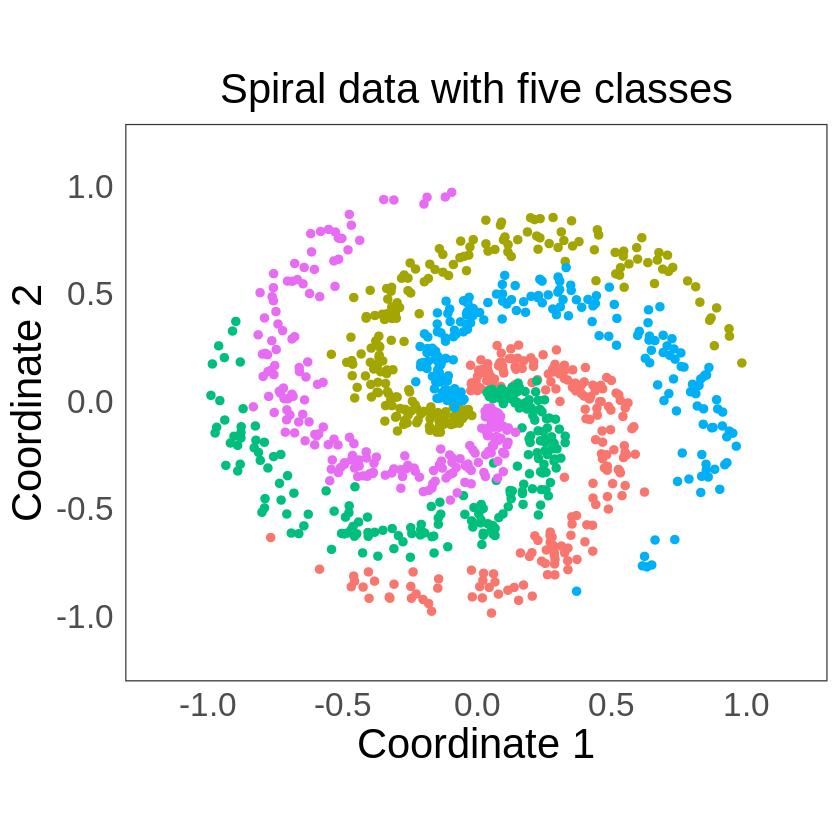
We consider a spiral data set inspired by (Guan et al., 2019; Amiri et al., 2015; Helfmann et al., 2018). The dimensionality is , and index set is partitioned into five classes with identical cardinalities: . Denoting the Hadamard product between two vectors by and the normal distribution with mean and standard deviation by , we construct the data as follows: for each class , we set
, and , where the elements of and are given by and for and . Each element of each input vector is then divided by the maximum among the elements of that vector, so that for all and . The data are visualized in Figure 2.
To fit these data, we consider a two-layer ReLU network with uniform width .
| Corrupted outputs (shuffled labels) | ||
| Prediction accuracies | ||
| 95.6 % | 95.6 % | |
| 95.2 % | 94.2 % | |
| 88.0 % | 79.6 % | |
| 85.6 % | 73.2 % | |
| Corrupted inputs | ||
| Prediction accuracies | ||
| 95.6 % | 95.6 % | |
| 95.6 % | 95.6 % | |
| 93.8 % | 90.2 % | |
rivals or outperforms in all settings
Data corruptions
We corrupt the spiral data in two ways:
Corrupted labels: The labels for are changed to other class labels.
Corrupted inputs: The elements of the input vectors for outliers are subjected to additional perturbations as described in Section 5.2.
Error quantification
The first half of the samples will be used for training, while the other half will be used for testing. For the estimator , which is computed by minimizing the mean of on the training data, the generalization accuracy is calculated, where is the indicator function defined by
We define as in Section 5.2, where the number of blocks can range in .
Results and conclusions
Table 6 summarizes the results for various settings. To begin, we see that DeepMoM and estimators behave very similarly in the case of uncorrupted and slightly corrupted labels () and slightly corrupted inputs (). But when the corruptions are more serious, our DeepMoM estimator clearly outperforms the other approaches. In general, we conclude that is efficient on benign data and robust on problematic data.
6 Discussion
Our new approach to training the parameters of neural networks is robust against corrupted samples and yet leverages informative samples efficiently. We have confirmed these properties numerically in Sections 2, 5.2, and 5.3. The approach can, therefore, be used as a general substitute for basic least-squares-type or cross-entropy-type approaches.
We have restricted ourselves to feed-forward neural networks with ReLU activation, but there are no obstacles for applying our approach more generally, for example, to convolutional networks or other activation functions. However, to keep the paper clear and concise, we defer a detailed analysis of in other deep-learning frameworks to future work.
Similarly, we model corruption by uniform or heavy-tailed random perturbations of the inputs or outputs or by randomly swapping labels, but, of course, one can conceive a plethora of different ways to corrupt data.
In sum, given modern data’s limitations and our approach’s ability to make efficient use of such data, we believe that our method can have a substantial impact on deep-learning practice, and that our paper can spark further interest in robust deep learning.
Acknowledgements
We thank Guillaume Lecué, Timothé Mathieu, Mahsa Taheri, and Fang Xie for their insightful inputs an suggestions.
References
- Akhtar and Mian, (2018) Akhtar, N. and Mian, A. (2018), “Threat of adversarial attacks on deep learning in computer vision: a Survey,” arXiv:1801.00553.
- Amiri et al., (2015) Amiri, S., Clarke, B., and Clarke, J. (2015),, On the efficiency of Hybrid clustering to achieve the clustering.
- Arazo et al., (2019) Arazo, E., Ortego, D., Albert, P., O’Connor, N., and Mcguinness, K. (2019), “Unsupervised label noise modeling and loss correction,” Proceedings of the 36th international conference on machine learning, 97, 312–321.
- Athalye et al., (2018) Athalye, A., Engstrom, L., Ilyas, A., and Kwok, K. (2018), “Synthesizing Robust Adversarial Examples,” arXiv:1707.07397.
- Barron, (2019) Barron, J. (2019), “A general and adaptive robust loss function,” arXiv:1701.03077.
- Belagiannis et al., (2015) Belagiannis, V., Rupprecht, C., Carneiro, G., and Navab, N. (2015), “Robust optimization for deep regression,” arXiv:1505.06606.
- Brückner et al., (2012) Brückner, M., Kanzow, C., and Scheffer, T. (2012), “Static prediction games for adversarial learning problems,” Journal of machine learning research, 13, 85, 2617–2654.
- cancer institute, (2006) cancer institute, National (2006), “TCGA database,” GDC data portal.
- Carlini and Wagner, (2017) Carlini, N. and Wagner, D. (2017), “Adversarial examples are not easily detected: bypassing ten detection methods,” arXiv:1705.07263.
- Dillies et al., (2012) Dillies, M.-A., Rau, A., Aubert, J., Hennequet-Antier, C., Jeanmougin, M., Servant, N., Keime, C., Marot, G., Castel, D., Estelle, J., Guernec, G., Jagla, B., Jouneau, L., Laloë, D., Le Gall, C., Schaëffer, B., Le Crom, S., Guedj, M., and Jaffrézic, F. (2012), “A comprehensive evaluation of normalization methods for Illumina high-throughput RNA sequencing data analysis,” Briefings in Bioinformatics, 14, 6, 671–683.
- Friedrich et al., (2020) Friedrich, S., Antes, G., Behr, S., Binder, H., Brannath, W., Dumpert, F., Ickstadt, K., Kestler, H., Lederer, J., Leitgöb, H., Pauly, M., Steland, A., Wilhelm, A., and Friede, T. (2020), “Is there a role for statistics in artificial intelligence?,” arXiv:2009.09070.
- Goodfellow et al., (2018) Goodfellow, I., McDaniel, P., and Papernot, N. (2018), “Making machine learning robust against adversarial inputs : such inputs distort how machine-learning based systems are able to function in the world as it is,” Communications of the ACM, 61, 7, 56–66.
- Goodfellow et al., (2015) Goodfellow, I., Shlens, J., and Szegedy, C. (2015), “Explaining and harnessing adversarial examples,” arXiv:1412.6572.
- Guan et al., (2019) Guan, J., Hsieh, F., and Koehl, P. (2019), “DCG++: a data-driven metric for geometric pattern recognition,” PLoS ONE, 14.
- Hampel et al., (2011) Hampel, F., Ronchetti, E., Rousseeuw, P., and Stahel, W. (2011), Robust statistics: the approach based on influence functions, Wiley.
- He et al., (2017) He, W., Wei, J., Chen, X., Carlini, N., and Song, D. (2017), “Adversarial example defenses: ensembles of weak defenses are not strong,” arXiv:1706.04701.
- Helfmann et al., (2018) Helfmann, L., Lindheim, J., Mollenhauer, M., and Banisch, R. (2018), “On Hyperparameter Search in Cluster Ensembles,” ArXiv:abs/1803.11008.
- Huber, (1964) Huber, P. (1964), “Robust estimation of a location parameter,” Annals of mathematical statistics, 35, 1, 73–101.
- Huber and Ronchetti, (2009) Huber, P. and Ronchetti, E. (2009), Robust statistics, Wiley.
- Jiang et al., (2018) Jiang, L., Zhou, Z., Leung, T., Li, L.-J., and Li, F.-F. (2018), “MentorNet: learning data-driven curriculum for very deep neural networks on corrupted labels,” arXiv:1712.05055.
- keen security lab, (2019) keen security lab, Tencent (2019), “Experimental security research of Tesla Autopilot,” Tencent keen security lab.
- Kos and Song, (2017) Kos, J. and Song, D. (2017), “Delving into adversarial attacks on deep policies,” arXiv:1705.06452.
- Kurakin et al., (2016a) Kurakin, A., Goodfellow, I., and Bengio, S. (2016a), “Adversarial examples in the physical worlda,” arXiv:1607.02533a.
- Kurakin et al., (2016b) — (2016b), “Adversarial machine learning at scaleb,” arXiv:1611.01236b.
- Le Cam, (1973) Le Cam, L. (1973), “Convergence of estimates under dimensionality restrictions,” The annals of statistics, 1, 1, 38–53.
- Le Cam, (1986) — (1986), “Sums of independent random variables,” Asymptotic methods in statistical decision theory springer series in statistics, 399–456.
- Lecué and Lerasle, (2017a) Lecué, G. and Lerasle, M. (2017a), “Learning from MOM’s principles: Le Cam’s approacha,” arXiv:1701.01961a.
- Lecué and Lerasle, (2017b) — (2017b), “Robust machine learning by median-of-means : theory and practiceb,” arXiv:1711.10306b.
- Lecué et al., (2020) Lecué, G., Lerasle, M., and Mathieu, T. (2020), “Robust classification via MOM minimization,” Machine learning, 109, 8, 1635–1665.
- Lederer, (2020) Lederer, J. (2020), “Risk bounds for robust deep learning,” arXiv:2009.06202.
- Lederer, (2021) — (2021), “Activation functions in artificial neural networks: a systematic overview,” arXiv:2101.09957.
- Liu and Belkin, (2019) Liu, C. and Belkin, M. (2019), “Accelerating SGD with momentum for over-parameterized learning,” arXiv:1810.13395.
- Lugosi and Mendelson, (2019a) Lugosi, G. and Mendelson, S. (2019a), “Regularization, sparse recovery, and median-of-means tournamentsa,” Bernoullia, 25, 3.
- Lugosi and Mendelson, (2019b) — (2019b), “Risk minimization by median-of-means tournamentsb,” Journal of the European mathematical societyb, 22, 3, 925–965.
- Madry et al., (2017) Madry, A., Makelov, A., Schmidt, L., Tsipras, D., and Vladu, A. (2017), “Towards deep learning models resistant to adversarial attacks,” arXiv:1706.06083.
- Madry et al., (2019) — (2019), “Towards deep learning models resistant to adversarial attacks,” arXiv:1706.06083.
- Papernot et al., (2015) Papernot, N., McDaniel, P., Wu, X., Jha, S., and Swami, A. (2015), “Distillation as a defense to adversarial perturbations against deep neural networks,” arXiv:1511.04508.
- Patrini et al., (2017) Patrini, G., Rozza, A., Menon, A., Nock, R., and Qu, L. (2017), “Making deep neural networks robust to label noise: a loss correction approach,” arXiv.
- Roh et al., (2021) Roh, Y., Heo, G., and Whang, S. (2021), “A survey on data collection for machine learning: a big data - AI integration perspective,” IEEE transactions on knowledge and data engineering, 33, 4, 1328–1347.
- Rumelhart et al., (1986) Rumelhart, D., Hinton, G., and Williams, R. (1986), “Learning representations by back-propagating errors,” Nature, 323, 6088, 533–536.
- Salman et al., (2019) Salman, H., Yang, G., Li, J., Zhang, P., Zhang, H., Razenshteyn, I., and Bubeck, S. (2019), “Provably robust deep learning via adversarially trained smoothed classifiers,” arXiv:1906.04584.
- Sharif et al., (2016) Sharif, M., Bhagavatula, S., Bauer, L., and Reiter, M. (2016), Accessorize to a crime: real and stealthy attacks on state-of-the-art face recognition, Proceedings of the 2016 ACM SIGSAC conference on computer and communications security.
- Su et al., (2019) Su, J., Vargas, D., and Sakurai, K. (2019), “One pixel attack for fooling deep neural networks,” IEEE transactions on evolutionary computation, 23, 5, 828–841.
- Sun, (2019) Sun, R. (2019), “Optimization for deep learning:theory and algorithms,” arXiv:1912.08957.
- Torrenté et al., (2020) Torrenté, L., Zimmerman, S., Suzuki, M., Christopeit, M., Greally, J., and Mar, J. (2020), “The shape of gene expression distributions matter: how incorporating distribution shape improves the interpretation of cancer transcriptomic data,” BMC Bioinformatics, 21.
- Tramèr and Boneh, (2019) Tramèr, F. and Boneh, D. (2019), “Adversarial training and robustness for multiple perturbations,” arXiv:1904.13000.
- Tramèr et al., (2017) Tramèr, F., Kurakin, A., Papernot, N., Goodfellow, I., Boneh, D., and McDaniel, P. (2017), “Ensemble adversarial training: attacks and defenses,” arXiv:1705.07204.
- Tsipras et al., (2019) Tsipras, D., Santurkar, S., Engstrom, L., Turner, A., and Madry, A. (2019), “Robustness may be at odds with accuracy,” arXiv:1805.12152.
- Wang and Yu, (2019) Wang, H. and Yu, C.-N. (2019), “A direct approach to robust deep learning using adversarial networks,” arXiv:1905.09591.
- Wang et al., (2018) Wang, T., Gu, Y., Mehta, D., Zhao, X., and Bernal, E. (2018), “Towards robust deep neural networks,” arXiv:1810.11726.
- Wang et al., (2016) Wang, Z., Chang, S., Yang, Y., Liu, D., and Huang, T. (2016), “Studying very low resolution recognition using deep networks,” arXiv:1601.04153.
- Wong and Kolter, (2018) Wong, E. and Kolter, J. (2018), “Provable defenses against adversarial examples via the convex outer adversarial polytope,” arXiv:1711.00851.
- Xu and Mannor, (2010) Xu, H. and Mannor, S. (2010), “Robustness and generalization,” arXiv:1005.2243.
- Yi and Wu, (2019) Yi, K. and Wu, J. (2019),, Probabilistic end-To-end noise correction for learning with noisy labels. in Proceedings of the IEEE/CVF conference on computer vision and pattern recognition.
- Yuan et al., (2019) Yuan, X., He, P., Zhu, Q., and Li, X. (2019), “Adversarial examples: attacks and defenses for deep learning,” IEEE transactions on neural networks and learning systems, 30, 9, 2805–2824.