A Sum-of-Ratios Multi-Dimensional-Knapsack Decomposition for DNN Resource SchedulingThanks: This work has been supported in part by NSF grants CAREER CNS-1943226, CCF-1758736, ONR grant N00014-17-1-2417, a Google Faculty Research Award, NSF CNS-1651947, and Hong Kong RGC grants HKU 17204619, 17208920.
Abstract
In recent years, to sustain the resource-intensive computational needs for training deep neural networks (DNNs), it is widely accepted that exploiting the parallelism in large-scale computing clusters is critical for the efficient deployments of DNN training jobs. However, existing resource schedulers for traditional computing clusters are not well suited for DNN training, which results in unsatisfactory job completion time performance. The limitations of these resource scheduling schemes motivate us to propose a new computing cluster resource scheduling framework that is able to leverage the special layered structure of DNN jobs and significantly improve their job completion times. Our contributions in this paper are three-fold: i) We develop a new resource scheduling analytical model by considering DNN’s layered structure, which enables us to analytically formulate the resource scheduling optimization problem for DNN training in computing clusters; ii) Based on the proposed performance analytical model, we then develop an efficient resource scheduling algorithm based on the widely adopted parameter-server architecture using a sum-of-ratios multi-dimensional-knapsack decomposition (SMD) method to offer strong performance guarantee; iii) We conduct extensive numerical experiments to demonstrate the effectiveness of the proposed schedule algorithm and its superior performance over the state of the art.
I Introduction
In recent years, deep-learning-based applications are quickly finding their ways into our everyday life, including healthcare, automobile, retail, smart homes, just to name a few. However, these applications also generate and inject a large volume of resource-intensive computing jobs for training deep neural networks (DNNs), which are used in various systems for computer vision, natural language processing, online recommendation, etc. In order to sustain such a rapidly growing need for DNN training in recent years, it is widely accepted that a viable solution is to exploit the vast parallelism in distributed computing architectures to schedule deep learning jobs. To date, however, most traditional resource scheduling schemes for computing clusters are not designed for DNN training (e.g., Google’s Borg System [1] employs static resource allocation specified by the users upon job submissions). Also, most of the recently proposed scheduling schemes designed for DNN jobs (e.g., Gandiva [2] and Tiresias [3]) are heuristic approaches, which provide no performance guarantee. In light of the increasing importance of DNN-based applications, there is a pressing need for developing provably efficient resource schedulers tailored for DNN training in computing clusters.
However, developing such resource scheduling algorithms for DNN training clusters is highly non-trivial. In a computing cluster, DNN training jobs are submitted over time with various competing resource requirements (numbers of CPUs and GPUs, size of memory, etc.), and the training process is both resource-intensive and time-consuming. For example, researchers showed that it could take 115 minutes to train a model with ResNet50 dataset [4] on a DGX-1 machine with 8 V100 GPUs [5], and even 3–5 days to train the DeepSpeech2 model [6] on the LibriSpeech dataset [7] using 16 GPUs [6]. Also, to date, there is a lack of a tractable and accurate analytical model that takes different mechanisms of communication-computation overlapping into consideration based on the layered structure of DNN.11 1 To speed up the training process, the idea of exploiting the special layered structure of DNNs to overlap communication and computation has been explored recently in[8, 9, 10], which showed that the training throughput of the MXNet framework could be improved by 25%–70%. Furthermore, similar to the design of most scheduling algorithms for large-scale distributed computing clusters, the computing resource limitation for DNN computing jobs naturally leads to integer bin-packing-like constraints in the scheduling problem, which makes the problem NP-Hard. Also, the objective function of the DNN resource scheduling problem has a sum-of-ratios structure due to the computational speed characterization in DNN training. As a result, the scheduling problem is non-convex even with continuous relaxation, which introduces yet another layer of difficulty to the already-challenging problem.
In this paper, we overcome the above challenges and develop a suite of scheduling algorithmic techniques for efficient DNN training in computing clusters Our main results and technical contributions are summarized as follows:
- •
We develop a new performance analysis framework for scheduling DNN training jobs. Specifically, we first propose a unified analytical model to characterize the DNN training, which captures a variety of ways to overlap communication and computation by exploiting the layered structure of DNNs.We then formulate the job admission and resource scheduling problem for DNN training by associating the above unified analytical model with both synchronous and asynchronous stochastic gradient descent (SGD) algorithms. Each job is associated with a utility function, which is non-increasing with respect to its job completion time. The objective of the analytical model is to maximize the overall utility (i.e., minimize the overall training completion time).
- •
Based on the above analytical framework, we formulate the resource scheduling problem as a mixed-integer nonlinear programming problem (MINLP), and prove its NP-hardness. To overcome this fundamental hardness, we propose a divide-and-conquer approach called SMD (sum-of-ratio multi-dimensional-knapsack decomposition). Specifically, based on a keen observation of the physical reality of resource requests in most distributed cloud computing systems in practice (e.g., Amazon’s EC2), we show that our resource scheduling problem has a decomposition structure. Under this decomposition, the inner subproblem is a mixed-integer sum-of-ratios problem with packing constraints. Thanks to the lower dimensionality of the inner subproblem, we are able to develop an efficient -approximation algorithm based on grid-searching coupled with randomized rounding for solving this subproblem.
- •
Upon solving the inner subproblem, we show that the outer subproblem reduces to a multi-dimensional knapsack problem (MKP), which also admits an efficient -approximation algorithm. By combining both steps, we establish the overall approximation ratio of the proposed SMD approach. To verify the efficacy of our proposed algorithm, we conduct numerical experiments based on Google cluster traces [11]. Our results show that the proposed SMD approach significantly outperforms the equal server-worker allocation scheme (widely used in practice) and a state-of-the-art approach called Optimus [12].
The remainder of this paper is organized as follows. In Section II, we review the literature to put our work in a comparative perspective. In Section III, we introduce the system model and problem formulation. Section IV presents our algorithms and their performance analysis. Section V shows numerical results, and Section VI concludes this paper.
II Related Work
Due to the rise of machine learning (ML) applications and their high computational workload, optimizing resource scheduling to facilitate distributed ML frameworks have attracted a great amount of interest in recent years (see, e.g., [13, 14, 15, 16] and the references therein). DNN training jobs have unique characteristics (e.g., iterativeness and layered structure), which could be leveraged to overlap computation and communication time between iterations to reduce the training time. However, these existing works were designed for resource allocation to support general ML jobs in computing clusters, which may not be tailored for DNN training jobs. As a result, when being applied in DNN training, their performance is suboptimal in general since they do not leverage the aforementioned characteristics of DNN training.
To date, research on computing cluster scheduling optimization tailored for DNN training remains relatively new with limited results. Most of the early attempts in this area (e.g., [17] and references therein) only considered static allocation of workers and parameter servers (PS). To our knowledge, Yan et al. [18] was the first to investigate the performance of distributed ML frameworks, and developed a DNN performance model at a layer-level granularity (e.g., the model considers the computation time of each operator on a specific CPU and the NN structures). Subsequently, Gandiva [2] exploited intra-job predictability to time-slice GPUs efficiently across multiple jobs to better-fit GPUs. Tiresias [3] aimed to reduce the job completion times when the jobs’ execution times are unpredictable due to non-smooth loss curves during a trial-and-error exploration. The most recent work [19] focused on making machine learning workloads complete in a finish-time fair manner. However, these schedulers are based on heuristic approaches. Also, the training completion time of a job is significantly affected by resource allocation. Studies in [20] showed that increasing resources did not contribute to a linear increase of the training speed and could even slow down the training process. Since static numbers of workers and PSs specified by users are suboptimal in general, researchers have also started to consider dynamic scheduling algorithms to determine optimal numbers of workers and PSs to optimize the training speed. To our knowledge, the first dynamic scheduling algorithm with performance guarantee was reported by Bao et al. [21], where they designed an online scheduling algorithm for deep learning jobs. However, their studies relied on strong assumptions and simplified modeling of deep learning jobs.
The most related work to ours is Optimus [20], where Peng et al. developed a heuristic resource allocation algorithm for the distributed deep learning jobs. Our work differs from [20] in the following key aspects: 1) In [20], the authors built the performance model without taking the DNN layered structure into consideration. As will be shown later, this yields suboptimal scheduling decisions in general. By contrast, we develop an analytical model that considers the layered characteristics of DNN training, which captures communication-computation overlapping in state-of-the-art DNN training systems [9]; and 2) Optimus proposed a dynamic resource scheduler, which is only a heuristic with no performance guarantee based on their online-fitted resource-performance models. In comparison, we propose a resource scheduler that leverages an analytical model to offer strong performance guarantees.
III System Model and Problem Formulation
In this section, we first present our general problem formulation for DNN training in distributed computing clusters in Section III-A. We then specialize the problem formulation under both synchronous and asynchronous SGD with the basic sequential training model [22] in Section III-B. Lastly, in Section III-C, we further generalize and refine our analytical model to include two more advanced DNN training models.
III-A General Problem Formulation


In this paper, we focus on data parallelism in data centers with the PS architecture [23, 24]22 2 Due to the homogeneous processing speed in data centers, we assume that the straggling issue is minor in this paper.. As shown in Fig. 2, in each iteration, each worker fetches a mini-batch of samples from its local dataset and computes a stochastic gradient. Upon finishing computation, each worker sends the gradient to the PSs to update the model parameters following an optimization algorithm, e.g., the stochastic gradient descent (SGD) method. The workers then will pull the updated parameters from the PSs, fetch the next mini-batch of samples and proceed to the next iteration. This process repeats until some convergence criterion of the optimization algorithm is met.
The gradient computation at each worker is based on the specific DNN as illustrated in Fig. 2. In each iteration, one mini-batch of samples is used by a worker to compute the loss from the initial layer to the last layer, which is referred to as forward propagation (FP). After FP, a stochastic gradient of the DNN model parameters will be computed in the reverse order of layers in a backward propagation (BP) fashion. The computed gradients are used for updates at the PSs.
We consider the setting where DNN training jobs are submitted by users to the computing cluster to be processed periodically. These submitted jobs are trained using workers and PSs implemented via virtual machines or containers, which share resources in the underlying servers. Upon submission, the user will specify the resource needed for the job, based on which our algorithm will determine the numbers of workers and PSs if the job is admitted in the current scheduling interval. The jobs that are submitted during the scheduling interval are called active jobs. We assume that the scheduling interval is sufficiently large (e.g., hours) such that all the scheduled active jobs can be completed within a scheduling interval.
We use to denote the total number of iterations to train for job , which is specified by the user.33 3 In practice, to prevent spending excessively long time waiting for the training process of a DNN job to converge, a maximum number of training iterations is usually set by the user. We use to denote the current training speed of job (i.e., the number of iterations completed per unit time), which is a function of the number of PSs () and the number of workers (). Then, the completion time of job can be estimated as . Let denote the set of active jobs submitted in the scheduling interval with , and denote the set of computing resources (e.g., CPU, GPU and memory). Let and be the amount of type- resources demanded by a worker and a PS for job , respectively. Let be the resource limit specified by the user for job , i.e., the maximum amount of resource the user may need. Let denote the capacity of type- resource in the computing cluster. Due to resource limits in the cluster, the system may not be able to process all jobs in in the current scheduling interval. Thus, we use a binary variable to indicate whether job is admitted in this interval () or not (). Let be the utility function associated with job , which is non-increasing with respect to the completion time . In this paper, our goal is to optimize the admission decision and resource allocation decisions and to maximize the overall utility for the submitted jobs in each scheduling interval. This optimization problem can be formulated as:
| (1) | ||||
| subject to | (2) | |||
| (3) | ||||
III-B Training Speed Modeling
In the general problem formulation above, the training speed function remains to be defined. Next, we will first derive the training speed per iteration per worker based on the basic sequential computation-communication model [22], which will serve as a baseline for two more advanced computation-communication models in Sec. III-C.
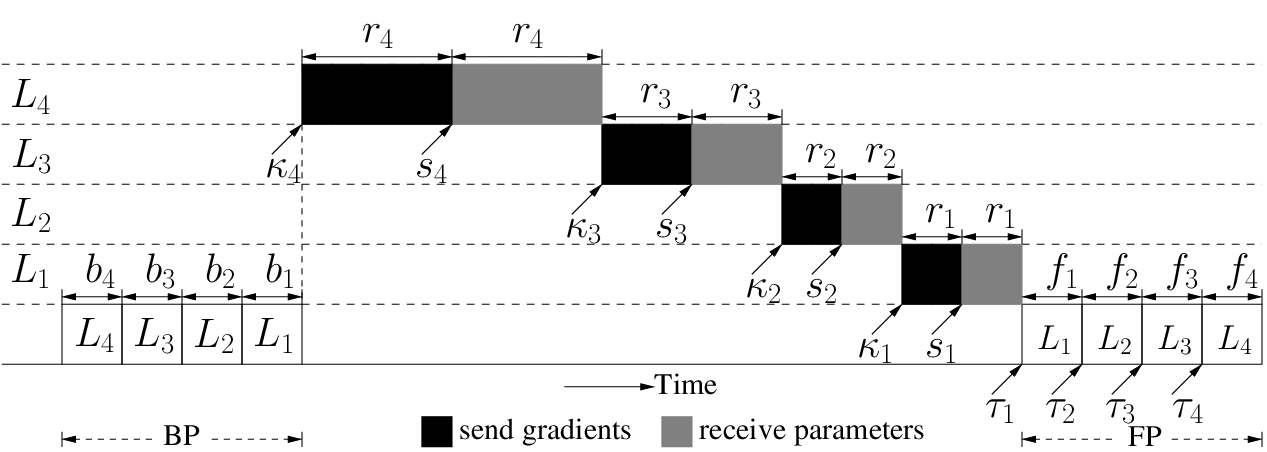
Notation: We let denote the number of layers in the DNN model of job . We use to denote the time spent for sending gradients to or receiving parameters from the PSs for layer of job (assuming equal time for pushing gradients and pulling updated parameters). Let and be the BP and FP computation times for layer of job , respectively. We use to denote the start time of sending gradients for layer of job , and we let be the start time of receiving parameters for layer of job . Let be the start time of FP for layer of job . For lighter notation, we will omit the job index “” in the subsequent training speed modeling if there is only one training job involved in the context (e.g., . We will revive “” if confusion may arise). Key notation is summarized in Table I for ease of reference.
| The set of active jobs in the scheduling interval | |||
|---|---|---|---|
| / | The set of PSs of job / The set of resource types | ||
| |||
| |||
| |||
| |||
| |||
| |||
| Start time of sending gradients of job at layer | |||
| |||
| |||
| |||
| # of layers in DNN model of job | |||
| / | # of training iterations for job / Model size of job | ||
| / | Global batch size of job / One mini-batch size of job | ||
| Capacity of type- resource in the DL cluster | |||
| Type- resource required by a worker in job | |||
| |||
| The resource limit specified by the user for job | |||
| / | # of workers of job / # of PSs of job | ||
| Bandwidth capacity of each PS of job | |||
| |||
| |||
|
The sequential model [22] is illustrated in Fig. 3, where push/pull of gradients/parameters start after BP of all layers are done, the push/pull of layers are done sequentially from the highest layer to the first layer, and FP of the next iteration starts after all push/pull are done. For an -layer DNN model, it is easy to see that the per-sample training time can be computed as . We let , , and denote the BP time, the communication time, and the FP time for processing a sample of job , respectively. Note that the key feature of the sequential model is that computation phases (i.e., BP and FP) and communication phases are conducted in a sequential fashion, which underutilizes the channel.


Consider a job with PSs and workers. We use to denote the bandwidth between each pair of PS and worker. Let be the model size (i.e., the number of elements in its gradient vector). Let be the mini-batch size. Then the FP time for processing a mini-batch can be calculated as . The BP time for processing a mini-batch does not depend on and can be computed as . We use to denote the average number of workers that send the computed gradients simultaneously to a PS , where denotes the set of PSs. Then, the bandwidth occupied by each worker is 44 4 In order to guarantee data transfer performance of each instance, it is common to reserve bandwidth for a VM/container for the accelerated computing in the cluster. For example, the reserved bandwidth of Amazon EC2 GPU instance P2 on AWS is 10Gbps or 25Gbps [25]. Thus we can safely assume that the workers have the same bandwidth. We use to denote the gradient size of layer and let be the corresponding number of PSs that layer will send its gradients to and receive its parameters from. For DNN models in practice, the number of neurons of a layer is usually much larger than the number of PSs, so it holds that . We also assume that is evenly divided into all PSs (implying ).55 5 For lower implementation complexity and managed overhead, most distributed ML frameworks (e.g., Tensorflow [26]) adopt roughly equal parameter allocation by default. Then, the time for sending gradients/receiving parameters under the symmetric assumption (equal communication speed for uplink and downlink) for each layer can be computed as: . It then follows that the data communication time can be computed as .
In addition to the communication and computation time, there exists extra communication overhead (e.g., establishing TCP connections) that increases linearly with the number of workers and PSs, which can be computed as , where and are constants that depend on the underlying system [20]. Thus, the per-iteration-per-mini-batch training time can be computed as Next, we derive the training speed function (i.e., how many iterations can be completed per unit time). We consider both synchronous and asynchronous trainings.
1) Synchronous Training: In synchronous training, PSs perform an update only after receiving gradients from all workers in each iteration. We let denote the global batch size, which is fixed throughout all iterations in synchronous training. Keeping a fixed global batch size is conformal to the standard SGD implementation, which is important for ensuring the same model result in the training process [27, 28]. We assume that is equally divided among all workers, which implies that the local batch size is . As a result, the training speed is equal to and can be modeled as [20]:
2) Asynchronous Training: In asynchronous training, once the PSs receive gradients from a worker, they immediately update their parameters. The expected number of steps completed by each worker in one time unit is . Thus, we can estimate the total number of steps performed by all workers in one time unit as . Since is proportional to the number of workers (i.e., the number of concurrent workers that send gradients to the same PS also increases as increases), we have for some . Hence, the training speed function can be modeled as [20]:
III-C Generalization to Advanced Training Models
In this subsection, we introduce two more advanced training models, namely, i) the wait-free model [22] and ii) the priority-based model [9], which overlap communication and computation to further reduce per-iteration delay. We remark that, although both models were not proposed by us, we are the first to quantitatively characterize the training speed for both models. Interestingly, it turns out that our training speed modeling for the sequential model can be generalized to these two more advanced communication-computation models (proofs of Lemmas 1 and 2 are omitted due to space limitation).66 6 All missing proofs can be found in our Tech Report [29].
1) Wait-free model [22]: As shown in Fig. 6, starting from the final layer, each layer takes turn to send gradients to the PSs immediately after finishing its own BP and the completion of gradient pushing of its subsequent layer. Compared to the sequential model, a key feature in this model is that part of the communication and computation can be conducted simultaneously. We derive per-sample training time as follows:
Lemma 1 (Wait-free model).
For the wait-free model, the start time of gradient-sending , for ; otherwise it is . The start time of parameter-receiving , for ; otherwise it is . The FP start time , for ; otherwise it is . It thus follows that the per-sample training time is .
Some important remarks for Lemma 1 are in order: 1) If the parameter size is skewed in the wait-free model, layers of larger sizes can introduce larger delay to layers of smaller sizes due to non-preemption. 2) In the wait-free model, only after receiving the updated parameters for the first layer, the FP of the next iteration can get started (see in Fig. 6); thus the gradient sending of the subsequent layers causes delays to the gradient sending of the initial layer, which in turn induces delay for the next iteration. Also, since the BP progresses in the reverse order of layers (i.e., from the last (output) layer to the first (input) layer), the gradients are also generated and sent in that order. As a result, no overlap between computation and communication is possible during FP (see Fig. 6).
2) Priority-based model [9]: An insight from the discussions above is that the closer a layer is to the input layer, the higher priority its gradient/parameter communication should have. The reason is that once the transmission of this layer is completed, the corresponding FP of this layer can start without waiting for all communications to be finished, thus significantly reducing delay. As shown in Fig. 6, the layer with a smaller index (i.e., closer to the input layer) always has a higher priority and its communication can preempt that of layers with larger indices. This induces further communication-computation overlapping and helps the next iteration get started as soon as possible.
Also, to better align communication and computation, the idea of “parameter slicing” can be used to mitigate the impact of skewed layer sizes. As shown in Fig. 6, we split each layer into smaller slices of size , whose communications can be further overlapped. Slices of the same layer have the same priority and the communication order of each slice within the same layer could be arbitrary.
We let be the end time of communication for layer of job . We derive the per-sample training time as follows:
Lemma 2 (Priority-based model).
For the priority-based model, the communication end time , if ; otherwise for and . The FP start time for and . It thus follows that the per-sample training time is .
Note that has a recursive property. Depending on whether the system is computation or communication dominant in each layer, Lemma 2 could lead to different expressions.
3) Unified expression for per-iteration training time: Note that, in both wait-free and priority-based model, the per-sample training time is DNN-dependent and determined by each layer’s size. Nonetheless, as long as the DNN of a training job is given, we can compute by using Lemmas 1 and 2. Also, we note that the communication-computation overlapping in wait-free and priority-based models effectively reduces the BP time, communication time, and FP time to certain fractions of those in the sequential model. Thus, the per-iteration training time of both models can be expressed as , where the coefficients are DNN-model-dependent.
We let , and be the FP time, BP time and communication time for processing a sample, respectively. Then these coefficients are defined as , , and . For instance, for the wait-free instance in Fig. 6, we can compute the coefficients as , , and . With this approach, the training speed function of a job under both synchronous training and asynchronous trainings can be generalized as:
| (4) | ||||
| (5) |
Note that the sequential model is a special case with , and . In the next section, we will see that these unified expressions in (4) and (5) enable us to design a suite of approximation algorithms to solve Problem (1).
IV Solution Approach
Due to the fundamental hardness of Problem (1) (to be shown soon), in this section, we will propose an approximation algorithmic approach, which we term sum-of-ratio multi-dimensional-knapsack decomposition (SMD), to solve this problem. In what follows, we will organize and present our approximation algorithmic approach in three main steps:
Step 1) Sum-of-Ratios Multi-Dimensional-Knapsack Decomposition (SMD): First, we note that in Problem (1), the resource scheduling decision variables are independent across jobs due to the fact that each summand in (1) only depends on each job . Therefore, we can decompose the problem into an inner subproblem and an outer subproblem as follows. First, by setting , the inner resource allocation sub-problem for job can be written as:
| (6) | ||||||
| subject to | (7) | |||||
| (8) | ||||||
Recall that the training speed function has different forms for synchronous and asynchronous trainings. Hence, Problem (6) can be further specialized as follows:
a) Synchronous training: In this case, we have:
| (9) | ||||||
| subject to |
where , , , , and .
b) Asynchronous training: In this case, we have:
| (10) | ||||||
| subject to |
where , , , and .
It is clear that Problem (6) is a mixed-integer nonlinear programming (MINLP) problem, which is NP-Hard in general [30]. In addition, even with continuous relaxation, it remains in the class of sum-of-ratios optimization problems, which is well-known to be NP-complete [31]. But thanks to the low dimensionality of the inner subproblem (a consequence of SMD), we will propose an -approximation algorithm for solving the inner subproblem. Upon solving (6), the outer subproblem reduces to selecting active jobs to be run in the current scheduling interval:
| (11) | ||||
| subject to |
Since is known after solving the inner subproblem, it is clear that the outer subproblem is a multi-dimensional knapsack problem (MKP) in essence. Therefore, in what follows, we will consider solving the inner sum-of-ratios subproblem and the outer MKP problem separately.
Step 2) Solving the inner sum-of-ratios subproblem: We first consider the inner subproblems (9) and (10) after relaxing the integrality constraint (8). Recall that the utility function is non-increasing. Thus, both problems can be equivalently reformulated as a sum-of-ratios problem with affine constraints, which can be written in the following general form:
| (12) | ||||
| subject to |
where , , and . We also note that in both problems , where denote the feasible domain of the problem. The sum-of-ratios problem with affine constraints is known to be NP-complete [31] but -approximation approach [32] exists.
Unlike the problem in [32] with covering constraints (may lead to unbounded search space), we exploit the special packing-like constraint structure in (7) to first obtain a tight upper bound for each ratio term to significantly reduce the search space. Specifically, we let , which is a linear fractional programming with non-empty and bounded feasible region . We choose the lower and upper bounds as and . Then transform the problem into a linear program using the Charnes-Cooper transformation [33], which then can be solved efficiently. Without loss of generality, we assume that the last summand has the largest ratio between the upper and lower bounds, i.e., . Then, the feasible domain for the summands is a polytope characterized as . We let and . Then, Problem (12) can be transformed into the following equivalent formulation:
| (13) | ||||
| subject to | ||||
We can see from the reformulated Problem (13) that, if a point is given, there is only one variable associated with the summand to be solved. Thus, the complexity of the problem is reduced significantly.
Step 2.1): Determining the Set of Grid Points: After finding the range for each summand in the objective function, we divide the polytope into smaller polytopes to perform a grid search, where the granularity is controlled by a precision parameter . We first find the largest integer number that does not exceed the upper bound of each summand when searching from the lower bound , i.e., . Then, we have the grid points set for each summand as . Next, by searching all the summands, we can obtain the search grid set as . It is clear that for any , we can always find a point , such that , thus can be approximated by the set .
Hence, Problem (13) can be solved by iterating over . For a given , the subproblem needs to be solved is as follows:
| (14) | ||||
| subject to | ||||
Notice that for a given , the term becomes a constant, then the equivalent formulation to Problem (14) is:
| (15) | ||||
| subject to |
which again can be transformed into a linear program using the Charnes-Cooper transformation [33] and solved efficiently.
The basic idea of the algorithm is first to perform the dimensionality reduction to reduce summands to terms, and then divide the feasible domain into smaller nonuniform grids. The feasible polytope domain obtained by finding the lower and upper bound of each summand is used to confine the space of grid points. Then, the original sum-of-ratios problem can be transformed and decomposed into a set of linear programming (LP) subproblems, each of which is associated with a grid point. As a result, the computational cost boils down to solving LP subproblems related to points in .
Note, however, that the total number of grid points still increases exponentially as the number of summands in (12) increases, which is intractable as the problem size gets large. Fortunately, we note that both inner problems (9) and (10) have just a few summands (four and three, respectively) thanks to SMD. Thus, it remains affordable to adopt a grid-search-based approach. By leveraging the special feature of cloud systems that each job has its reserved resources, we can reduce the high dimensionality of the problem and decompose it as in Problem (6). Thus, the problem is reduced to solving times of sum-of-linear-ratios with a small number of terms, which can be solved efficiently (Algorithm 1).
In Algorithm 1, we first obtain the grid points over the feasible domain in Line 1. We then iterate each point and update the objective and the fractional solution in Line 1 if the current objective value is smaller. Finally, we return the solution with the smallest objective value. Following similar analysis as in [32] (hence omitted for brevity), we can show that Algorithm 1 is an -approximation.
Upon solving the continuous relaxation of inner sum-of-ratios subproblems (9) and (10), it remains to obtain an integer solution to calculate the utility. This is still an NP-Hard integer programming problem with generalized packing-type constraints in (7). We propose the following solution approach: First, we solve the continuous relaxation of , where , , and . Let be the obtained fractional optimal solution. Then, we propose a randomized rounding scheme as shown in Alg. 2 to round and arrive at an integer solution.
Step 3) Solving the outer MKP subproblem: The general formulation of the outer MKP subproblem can be written as:
| (16) | ||||
where is the utility value of each job . Our goal is to select jobs that maximize the total utility among all the submitted jobs . The MKP problem is still a well-known NP-Hard problem [34] but admits an -approximation solution77 7 This -value is different and should not be confused with the in Step 2. that runs in polynomial time if and are fixed. Here, we adopt the -approximation scheme [35] to our problem setting. We let , for . Let be the linear program obtained from Problem (16) by setting , if ; and set it to , if . Let be an optimal basic feasible solution to . The main idea of this approach is to solve for all . Then, we round down the solution . Finally, we return the best solution with the largest objective value. The difference between and is small since is a fixed small number in our case.
IV-A Performance Analysis
We now examine the overall approximation ratio of our proposed algorithms. Note that the key component in our algorithm is the proposed randomized rounding scheme in Algorithm 2 for Problem (6). Thus, we first prove the following result for the randomized rounding algorithm (proofs are omitted due to space limitation).
Lemma 3 (Rounding).
Let . Let L be the number of sum-of-ratios terms. Pick some constant , and define as:
With probability greater than , achieves a cost at most times the cost of , and .
Note that is used for characterizing the randomized rounding algorithm’s performance. Lemma 3 indicates that with probability , one achieves an approximation ratio at most with the stated probabilistic feasibility guarantee. From the statement, we can see that the approximation ratio is ultimately determined by , since increases as increases. Thus, if one desires a better approximation ratio, then a larger should be picked. That is, there exists a trade-off between the approximation ratio value and its achieving probability, both of which are quantified by .
The approximation ratio of our algorithm is the worst-case upper bound of the ratio between the overall utility of admitted jobs obtained by the optimal solution of Problem (1) and the total utility achieved by Algorithm SMD in the overall time horizon. By specializing Lemma 3 with parameters in Problem (6), we have the following result for Algorithm 2:
Theorem 4 (Approximation Ratio of Rounding in Alg. 2).
Let and be the performance ratios of solving the sum-of-ratios problem and MKP, respectively, where . Let and be defined as in Lemma 3. Let be the completion time of job and be the optimal completion time of job . Let be chosen as in Alg. 2. We let , and let . Following Theorem 4, we can establish the overall approximation ratio and running time complexity of the SMD approach as follows:
Theorem 5 (Overall Approximation Ratio of SMD).
With probability greater than , the proposed SMD-based method returns a feasible solution with -approximation performance guarantee.
Theorem 6 (Polynomial Running Time).
We let and be the time complexity for solving the sum-of-ratios problem under synchronous and asynchronous training of job , respectively, which can be solved in polynomial time [32]. Let . Let be the time complexity for MKP problem, which is polynomial [35]. Then, the overall time complexity of Algorithm SMD is .


V Numerical Evaluation
We conduct simulation studies to evaluate the efficacy of our proposed algorithms. In our simulation, the computing cluster follows the real-world system in[36] with job parameters generated uniformly at random from the following intervals: , MB, , , . We consider four types of resources: GPU, CPU, memory and storage. For fair comparisons, we use similar settings as in [24] [17] [16] and set resource demands of each worker as: 0–4 GPUs, 1–10 vCPUs, 2–32 GB memory, and 5–10GB storage. We set resource configuration of each PS as: 1–10 vCPUs, 2–32GB memory and 5-10GB storage. We set bandwidth capacity of each PS to Gbps. Capacities of virtual instances to run workers/PSs are set according to resource configuration of Amazon EC2 C4 instances. We set the resource limit of each job to times of the resource limit of each instance with (according to the reality that each user is limited to a maximum of 20 instances per region in Amazon EC2). We set ms, ms and ms following the traces collected from the experiments in Optimus [20] based on Google cluster trace [11], which include jobs’ training losses, training speeds with various resource configuration, each server’s resource capacities, job configuration such as requirements of workers/PSs, as well as DL model specifications like parameter size. Then, we set and . We set , and following the tested values from Optimus [20]. We use a Sigmoid utility function [37, 20], with , and . Note that this range of corresponds to time-critical jobs [21].
We first compare our SMD algorithm with two baseline resource allocation policies: (1) ESW (setting the ratio of number of workers to number of PSs to 1:1 [38] for each job); and (2) Optimus [20] (compare the utility gain by adding one more worker and one more PS and choose the one with larger utility gain). Since Optimus estimates the training speed function based on an online learning approach by monitoring the convergence rate, we use our own speed function to estimate the utility for each job. We set , , and . To study how the total utility changes as the computing cluster resource capacity increases, we set one unit of resources as follows: (, , , ), and vary the resource capacity using 1-5 times of the unit resource. The comparison results under both Sync-SGD and Async-SGD are shown in Figs. 10–10. We can see that SMD significantly outperforms other policies and the gains in total utility becomes more pronounced as the number of jobs and resources in the computing cluster increases.
Next, we examine the approximation ratio of SMD. We evaluate the performance in terms of the ratio between the total utility obtained by our algorithm and the optimal total utility. The optimal utility is computed by enumerating all the possible combinations of numbers of workers and PSs for each job, and the combination with the largest utility will be returned. We vary the number of jobs per scheduling interval from to . We also set the cluster resource capacity as times of that of a virtual instance. The results are shown in Fig. 12. We can see that the ratio is much better than the theoretical bound and becomes larger as the number of jobs increases, which implies that our algorithm is scalable. Further, Sync-SGD has a worse approximation ratio since it is more sensitive to the changes of numbers of workers and PSs based on Eqn. (9) due to the linear term . In other words, the error introduced from the ”grid search” and randomized rounding when solving the inner sum-of-ratios-subproblem could lead to more utility loss compared to asynchronous training. Recall that the randomized rounding scheme is the key of our proposed Algorithm SMD. The packing constraints (7) are easier to satisfy with a smaller . Theorem 4 suggests that there is a trade-off: if we set to be close to one to pursue a better total utility result, the rounding time could be large to obtain a feasible solution. As becomes larger, the probability of violating the packing constraints increases, meaning that we need to have more rounding attempts to obtain an integer feasible solution. However, according to our numerical experiences, if the machine’s resource capacity is relatively large compared to the jobs’ resource demands per worker/PS, the number of rounding attempts is small and not sensitive to .
Lastly, we examine the actual used resources in our algorithm. A key feature of sum-of-ratios problems is that optimality is not necessarily obtained when the resource capacity constraints are binding. In other words, compared to the number of workers and parameter servers, the ratio between the number of workers and parameter servers plays a more critical role to minimize the training completion time. If such a better ratio can be found, it is possible that the system can save resources while having the same or even better performance in terms of the average training completion time. Hence, compared to other resource allocation policies that use as much resources specified by the user as possible, our SMD method may use much less resources while achieving the optimal performance. We let and vary the number of jobs per scheduling interval from to . We can see from Fig. 12 that the actual resources used is 30%-50% of that specified by the users. From the system’s perspective, the unused resources can be released and allocated to other jobs.
VI Conclusions
In this paper, we studied resource scheduling for DNN jobs in computing clusters. We demonstrated that the problem can be formulated as a non-convex integer non-linear program with bin-packing constraints, which is NP-Hard. We proposed an approximation scheduling algorithm based on a sum-of-ratios multi-dimensional knapsack (SMD) approach. Specifically, we developed a performance model that considers the special layered structure of DNN under different parameter synchronization mechanisms. Through careful investigation of the structure of the non-convex problem, we decomposed the problem based on SMD and proposed a suite of approximation techniques to solve the packing-type integer program with performance guarantees. Evaluation under realistic settings confirmed superior performances of SMD over existing works. DNN resource scheduling remains an under-explored area. Future extensions of this work may include, e.g., datacenter topology and communication contention among jobs.
References
- [1] A. Verma, L. Pedrosa, M. Korupolu, D. Oppenheimer, E. Tune, and J. Wilkes, “Large-scale cluster management at google with borg,” in Proc. of the 10th ACM European Conference on Computer Systems (Eurosys), 2015.
- [2] W. Xiao, R. Bhardwaj, R. Ramjee, M. Sivathanu et al., “Gandiva: Introspective cluster scheduling for deep learning,” in Proc. of USENIX OSDI, 2018.
- [3] J. Gu, K. G. Chowdhury, M. abd Shin, Y. Zhu, M. Jeon, J. Qian, H. Liu, and C. Guo, “Tiresias: A gpu cluster manager for distributed deep learning,” in NSDI, 2019.
- [4] K. He, X. Zhang, S. Ren, and J. Sun, “Deep residual learning for image recognition,” in Proceedings of IEEE Conference on Computer Vision and Pattern Recognition (CVPR), 2016.
- [5] “Mlperf training results.” [Online]. Available: https://mlperf.org/training-results-0-6/
- [6] E. B. Dario Amodei, Rishita Anubhai, C. Case, J. Casper, B. Catanzaro, J. Chen et al., “Deep speech 2: End-to-end speech recognition in english and mandarin,” in Proc. of the 33th International Conference on Machine Learning (ICML), 2016.
- [7] “Librispeech asr corpus.” [Online]. Available: http://www.openslr.org/12
- [8] S. H. Hashemi, S. A. Jyothi, and R. H. Campbell, “Tictac: Accelerating distributed deep learning with communication scheduling,” in Proceedings of Systems and Machine Learning (SysML), 2019.
- [9] J. W. Anand Jayarajan, G. Gibson, A. Fedorova, and G. Pekhimenko, “Priority-based parameter propagation for distributed dnn training,” in Proceedings of Systems and Machine Learning (SysML), 2019.
- [10] Y. Peng, Y. Zhu, Y. Chen, Y. Bao, B. Yi, C. Lan, C. Wu, and C. Guo, “A generic communication scheduler for distributed dnn training acceleration,” in Proceedings of the 27th ACM Symposium on Operating Systems Principles, 2019.
- [11] “Google cluster workload traces,” 2015. [Online]. Available: https://github.com/google/cluster-data
- [12] Y. Peng, Y. Bao, Y. Chen, C. Wu, and C. Guo, “Optimus: An efficient dynamic resource scheduler for deep learning clusters,” in Proc. of ACM EuroSys, 2018.
- [13] A. Ghodsi, M. Zaharia, B. Hindman, A. Konwinski, S. Shenker, , and I. Stoica, “Dominant resource fairness: Fair allocation of multiple resource types,” in Proc. of the 8th USENIX Symposium on Networked Systems Design and Implementation (NSDI), 2011.
- [14] S. A. Jyothi, C. Curino, I. Menache, S. M. Narayanamurthy et al., “Morpheus: Towards automated slos for enterprise clusters,” in Proc. of the 12th USENIX Symposium on Operating Systems Design and Implementation (OSDI), 2016.
- [15] A. Tumanov, T. Zhu, J. W. Park, M. A. Kozuch, M. HarcholBalter, and G. R. Ganger, “Tetrisched: Global rescheduling with adaptive plan-ahead in dynamic heterogeneous clusters,” in Proc. of the 11th ACM European Conference on Computer Systems (Eurosys), 2016.
- [16] P. Sun, Y. Wen, N. B. D. Ta, and S. Yan, “Towards distributed machine learning in shared clusters: A dynamically-partitioned approach,” in Proc. of IEEE Smart Computing, 2017.
- [17] T. M. Chilimbi, Y. Suzue, J. Apacible, and K. Kalyanaraman, “Project adam: Building an efficient and scalable deep learning training system,” in Proc. of USENIX OSDI, 2014.
- [18] F. Yan, O. Ruwase, Y. He, and T. Chilimbi, “Performance modeling and scalability optimization of distributed deep learning systems,” in Proc. of the 21th ACM International Conference on Knowledge Discovery and Data Mining (KDD), 2015.
- [19] K. Mahajan, A. Balasubramanian, A. Singhvi, S. Venkataraman, and A. Akella, “Themis: Fair and efficient gpu cluster scheduling,” in NSDI, 2020.
- [20] Y. Peng, Y. Bao, Y. Chen, C. Wu, and C. Guo, “Optimus: An efficient dynamic resource scheduler for deep learning clusters,” in Proc. of the 13th ACM European Conference on Computer Systems (Eurosys), 2018.
- [21] Y. Bao, Y. Peng, C. Wu, and Z. Li, “Online job scheduling in distributed machine learning clusters,” in Proc. of IEEE INFOCOM, 2018.
- [22] H. Zhang, Z. Zheng, S. Xu, W. Dai, Q. Ho, X. Liang, Z. Hu, J. Wei, P. Xie, and E. P. Xing2, “Poseidon: An efficient communication architecture for distributed deep learning on gpu clusters,” in In 2017 USENIX Annual Technical Conference (USENIX ATC 17), 2017, pp. 181–193.
- [23] J. Dean, G. S. Corrado, R. Monga, K. Chen, and others., “Large scale distributed deep networks,” in Proceedings of the 25th International Conference on Neural Information Processing Systems - Volume 1, ser. NIPS’12. USA: Curran Associates Inc., 2012, pp. 1223–1231.
- [24] M. Li, D. G. Andersen et al., “Scaling distributed machine learning with the parameter server,” in Proc. of USENIX OSDI, 2014.
- [25] “Amazon ec2 instances,” https://aws.amazon.com/ec2/instance-types/.
- [26] M. Abadi, P. Barham et al., “TensorFlow: A system for large-scale machine learning,” in Proc. of USENIX OSDI, 2016.
- [27] P. Goyal, P. Dolla, R. Girshick, P. Noordhuis, L. Wesolowski, A. Kyrola, A. Tulloch, Y. Jia, and K. He, “Accurate, large minibatch SGD: Training imagenet in 1 hour,” arXiv preprint arXiv:1706.02677, 2017.
- [28] M. S. Bazaraa, H. D. Sherali, and C. M. Shetty, Nonlinear Programming: Theory and Algorithms, 3rd ed. New York, NY: John Wiley & Sons Inc., 2006.
- [29] M. Yu, C. Wu, B. Ji, and J. Liu, “A sum-of-ratios multi-dimensional-knapsack decomposition for dnn resource scheduling,” Ohio State University, Tech. Rep., 2021. [Online]. Available: https://kevinliu-osu-ece.github.io/publications/ML_Networking_SMD_PERP’20.pdf
- [30] R. W. Freund and F. Jarre, “Solving the sum-of-ratios problem by an interior-point method,” in Journal of Global Optimization, 2001.
- [31] S. Schaible, “A note on the sum of a linear and linear‐fractional function,” in Naval Research Logistics Quarterly, 1977.
- [32] P. Shen, B. Huang, and L. Wang, “Range division and linearization algorithm for a class of linear ratios optimization problems,” in J. Comput. Appl. Math, vol. 350, 2019, pp. 324–342.
- [33] A. Chames and W. Cooper, “Programming with linear fractional functionals,,” in Naval Research Logistics Quarterly, 1962.
- [34] P. Chu and J. Beasley, “A genetic algorithm for the multidimensional knapsack problem,” in Journal of Heuristics, vol. 4, 1998, pp. 63–86.
- [35] A. FRIEZE and M. CLARKE, “Approximation algorithms for the m-dimensional 0-1 knapsack problem: Worst-case and probabilistic analysis,” in European Journal of Operational Research, vol. 15, 1984, pp. 100–109.
- [36] F. N. Iandola, M. W. Moskewicz, K. Ashraf, and K. Keutzer, “Firecaffe: Near-linear acceleration of deep neural network training on compute clusters,” in Proc. of IEEE CVPR, 2016.
- [37] Z. Huang, B. Balasubramanian, M. Wang, T. Lan, M. Chiang, and D. H. Tsang, “Need for speed: Cora scheduler for optimizing completiontimes in the cloud,” in Proc. of IEEE INFOCOM, 2015.
- [38] “Run deep learning with paddlepaddle on kubernetes,” 2017. [Online]. Available: https://kubernetes.io/blog/2017/02/run-deep-learning-with-paddlepaddle-on-kubernetes/