Directly profiling the dark-state transition density via scanning tunneling microscope

Introduction – Controllable light-matter interaction in the nanometer scale is one of the most fundamental and attractive topics in areas such as laser techniques (Haken 1984; Scully and Zubairy 1999), atom manipulation (Raab et al. 1987; Lett et al. 1988; Cohen-Tannoudji and Phillips 1990; Wieman et al. 1999), and cavity quantum electrodynamics (Dutra 2005; Walther et al. 2006; Agarwal 2013). Typically, the wavelength of the optical field is several orders of magnitude larger than the size of the matter of interest. In this region, the systems are essentially manipulated under the dipole interaction $\vec{\mathbf{\mu}}\cdot\vec{E}$, where $\vec{\mathbf{\mu}}$ is the electric dipole of the matter and $\vec{E}$ is the external electric field. Consequently, only the transitions between the atomic or molecular states with nonzero transition dipoles can be probed with electromagnetic field, leaving the dark state with zero transition dipole beyond the optical detection. For this reason, traditional optical spectroscopic approaches such as infrared (Stuart 2004), Raman (Larkin 2011), and fluorescence (Tanaka 2000; Romani et al. 2010) spectroscopies are not applicable for the detection of dark states. However, the molecular dark state plays a significant role in many biochemical processes, such as it helps to resist the photochemical damage to the deoxyribonucleic acid (DNA) induced by ultraviolet light (Middleton et al. 2009) and assist in the energy transfer process in the photosynthetic systems (Hashimoto et al. 2018; Feng et al. 2017).

The straightforward method is to break the dipole approximation with the spatial modulated field on the scale comparable to a single molecule. Such modulated field can be found near the tip of the scanning tunneling microscope (STM), which is as small as several atoms and able to induce electronic excitation which would have been forbidden under the dipole approximation. In contrast to optical excitation, the electronic excitation induced in STM provides detailed information on molecular states (Repp et al. 2005; Chen et al. 2010). By counting the luminescence photon, the scanning-tunneling-microscope-induced luminescence (STML) has emerged as a crucial tool for studying photoelectronic properties of single molecules (Rosławska et al. 2018; Nian et al. 2018; Imada et al. 2017; Doppagne et al. 2018; Chen et al. 2019; Kröger et al. 2018; Wu et al. 2019).

In this Letter, we show the scheme of directly profiling the dark-state transition details from STM (Dong et al. 2020) taking advantage of the localized electric field. We quantitatively demonstrate the resemblance between the relative inelastic current (luminescence photon counting) and the transition density profile of the dark-state transition.

Model –We demonstrate the basic setup of the model in Fig. 1(a), where a single molecule is placed on a NaCl-covered metal substrate. A metal tip scans over the molecule to allow the profiling. Driven at a nonzero bias voltage, an electron tunnels from one electrode to the other, while interacting with the molecule through the Coulomb interaction.

The total Hamiltonian consists of the tunneling electron Hamiltonian $\hat{H}_{\mathrm{el}}$, the molecular Hamiltonian $\hat{H}_{\mathrm{m}}$, and the electron-molecule interaction Hamiltonian $\hat{H}_{\mathrm{el-m}}$. The tunneling electron Hamiltonian is $\hat{H}_{\mathrm{el}}=-\hat{\nabla}^{2}/(2m_{e})+V(\hat{\vec{\mathbf{r}}})$, where $V(\hat{\vec{\mathbf{r}}})$ stands for the tunneling-electron potential at $\hat{\vec{\mathbf{r}}}=(x,y,z)$ and $m_{e}$ is the electron mass. The free tip and substrate wavefunctions are written as (Bardeen 1961; Gottlieb and Wesoloski 2006; Tersoff and Hamann 1983; Tersoff and Hamann 1985; Dong et al. 2020)

respectively. Here, $\hat{H}_{\mathrm{el,t}}$ ($\hat{H}_{\mathrm{el,s}}$) is the free tip (substrate) Hamiltonian without the corresponding potential in the substrate (tip) region. $\left|\phi_{k}\right\rangle\left(\left|\varphi_{n}\right\rangle\right)$ is the eigenfunction with eigenenergy $\widetilde{\xi}_{k}\equiv\xi_{k}+eV_{\mathrm{b}}\left(\widetilde{E}_{n}\equiv E_{n}\right)$, and $\xi_{k}\left(E_{n}\right)$ is its corresponding eigenenergy at zero bias voltage (Dong et al. 2020). The molecular Hamiltonian is simplified as a multi-level system $\hat{H}_{\mathrm{m}}=E_{g}\left|\chi_{g}\right\rangle\left\langle\chi_{g}\right|+\sum_{i=1}^{l}E_{e,i}\left|\chi_{e,i}\right\rangle\left\langle\chi_{e,i}\right|$, where $|\chi_{g}\rangle\>(|\chi_{e,i}\rangle)$ is its ground ($i$-th excited) state with energy $E_{g}\left(E_{e,i}\right)$ and $l$ is the total number of excited states.

The excitation of the molecules are performed through the electron-molecule interaction $\hat{H}_{\mathrm{el-m}}$ (Dong et al. 2020) as

where the transition matrix element

describes the transition matrix element from $\left|\phi_{k}\right\rangle\left(\left|\varphi_{n}\right\rangle\right)$ to $\left|\varphi_{n}\right\rangle\left(\left|\phi_{k}\right\rangle\right)$ in the subspace $\left|\chi_{g}\right\rangle,\left|\chi_{e,i}\right\rangle$, and $\hat{\sigma}_{x,i}\equiv\left|\chi_{e,i}\right\rangle\left\langle\chi_{g}\right|+\left|\chi_{g}\right\rangle\left\langle\chi_{e,i}\right|$ stands for the molecular transition. Here $\rho_{T,i}\left(\vec{q}\right)$ and $\rho_{n,k}\left(\vec{q}\right)$ are the Fourier transforms of the transition density $\rho_{T,i}\left(\vec{r}\right)\equiv\left\langle\vec{r}|\chi_{e,i}\right\rangle\left\langle\chi_{g}|\vec{r}\right\rangle$ and the product of the wavefunctions of the tip and the substrate $\rho_{n,k}\left(\vec{r}\right)\equiv\left\langle\vec{r}|\phi_{k}\right\rangle\left\langle\varphi_{n}|\vec{r}\right\rangle$, respectively. The transition dipole moment $\boldsymbol{\vec{\mu}}_{i}$ is obtained as the integral of the transition density $\rho_{T,i}\left(\vec{r}\right)$ and vector $\vec{r}$, i.e., $\boldsymbol{\vec{\mu}}_{i}=\int d^{3}\vec{r}\rho_{T,i}\left(\vec{r}\right)\vec{r}$. Detailed derivation is provided in Supplementary Material. Beyond the dipole approximation, the transition matrix element here is expressed as a convolution of the Fourier transform of the transition density and the electrode wavefunctions.

The properties of the molecules can be described by the tunneling current and the photon counting. The tunneling current is calculated to the first order ($\hat{H}_{\mathrm{el}}-\hat{H}_{\mathrm{el,s}}$ and $\hat{H}_{\mathrm{el-m}}$ as the perturbation). At the negative bias $V_{\mathrm{b}}<0$, the molecule is initially in its ground state and the electron is in the substrate eigenstate, i.e., $\left|\Psi\left(t=0\right)\right\rangle=\left|\chi_{g}\right\rangle\left|\varphi_{n}\right\rangle$. The wavefunction at time $t$ evolves as

Here $c_{g;k}\left(t\right)$ shows the probability amplitude of the elastic tunneling process and $c_{e,i;k}\left(t\right)$ the probability amplitude of the inelastic tunneling process. In the rotating-wave approximation, the inelastic tunneling amplitude becomes

where $E_{eg,i}\equiv E_{e,i}-E_{g}$ is the energy gap between the molecular states $\left|\chi_{g}\right\rangle$ and $\left|\chi_{e,i}\right\rangle$. By tracing out the degrees of freedom of the molecule, we obtain the inelastic current from $\left|\varphi_{n}\right\rangle$ to $\left|\phi_{k}\right\rangle$ as $\mathscr{J}_{n\rightarrow k}=\sum_{i=1}^{l}d\left|c_{e,i;k}\left(t\right)\right|^{2}/dt$ and the total inelastic current as

where

Here $\mu_{0}$ is the Fermi energy of the electrode and $\rho_{\mathrm{t}}\left(E\right)$ ($\rho_{\mathrm{s}}\left(E\right)$) is the density of state of the tip (substrate) at energy $E$. With the inelastic current at both negative and positive bias, we obtain the inelastic current as below (for the inelastic current at positive bias, see Supplementary Material)

Here $\mathrm{min}\left[E_{eg,i}/e\right]$ means the minimal $E_{eg,i}/e$ for all $i$. The condition for a nonzero inelastic current is $|eV_{\mathrm{b}}|>\mathrm{min}\left[E_{eg,i}\right]$ which is a generalized result of the $l=1$ model (Dong et al. 2020).

As shown in Eqs. (3) and (6), the inelastic tunneling current $I_{-\mathrm{,inela}}$ is a convolution of the square of the molecular transition density and the wavefunctions of the electrodes. It inherits the profile of the molecular transition density in the $x$-$y$ plane. Thus the molecule is more likely to get excited when the tip is above a larger transition density (absolute value). This submolecular-resolution feature has also been captured in the other two STML excitation mechanisms (Zhang et al. 2016; Imada et al. 2017; Wu et al. 2019; Kong et al. 2021), where only the bright-state excitation under the dipole approximation is studied. Beyond the dipole approximation, our theory predicts the dark-state excitation in the inelastic electron scattering (IES) mechanism. This discovery will provide a new platform for the study of molecular dark states.

General result of dark-state excitation – As a proof-of-principle example, we use a simplified molecule with only two levels, namely $l=1$. The transition density is assumed to be in a Gaussian form,

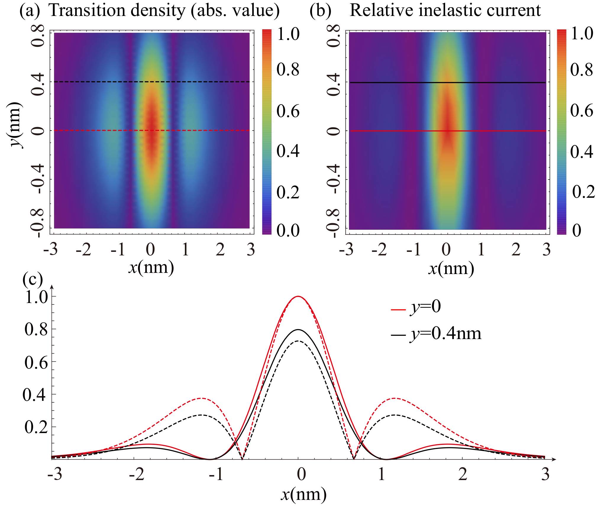
where $\sigma,\sigma_{1},\sigma_{2}$ are the width of the wave packets and $\delta\left(z\right)$ is the Dirac delta function. The transition density is assumed in the $x$-$y$ plane, shown in Fig. 2 (a)). The transition dipole is zero for the current dark state, i.e., $\int\vec{r}\rho_{T}(x,y,z)dxdydz=0$.

In the calculation, we assume the silver tip and substrate with the Fermi energy $\mu_{0}=-4.64$eV. The radius of the tip is $R=0.5$nm, and the distance between the molecular plane and the tip is $d=1$nm. The molecular energy gap between the ground and dark-excited state is $E_{eg}=2$eV. Here we choose $2\sigma_{1}=\sigma_{2}=\sigma=1$nm.

Fig. 2 shows the transition density (subfigure (a)) and the calculated tunneling current (subfigure (b)) from Eq. (7) with tip scanned in the $x$-$y$ plane. The bias voltage is set as $V_{\mathrm{b}}=-2.5$V to allow a non-zero current. The tunneling current profile resembles that of the transition density as shown in subfigure (a) and (b). We compare the tunneling current with the transition density at the cross section along $y=0$ and $0.4\mathrm{nm}$ in subfigure (c). The curves show the same trend with small deviation of the postions of the minima.

The main features of the inelastic current in the IES mechanism in Ref. (Dong et al. 2020) also appears in this work that goes beyond the dipole approximation. The minimal bias for nonzero inelastic current equals the molecule energy gap divided by the electron charge. The inelastic current at negative bias is larger than that at the positive bias (see Supplementary Material). The two features are typical in the IES mechanism in the cases with or without the dipole approximation.

Excitation of dark state of ZnPc – To show its capability in practical applications, we study the excitation of a zinc-phthalocyanine (ZnPc) molecule, widely used in the STML experiments (Zhang et al. 2016; Doppagne et al. 2018). Tab. (1) shows the transition dipoles and the energy gaps of the ZnPc molecule used in this paper. Due to the $D_{4h}$ symmetry of ZnPc (see the inset in Fig. 1 (a)), its first two excited states ($\mathrm{S}_{1}$ and $\mathrm{S}_{2}$) whose eigenenergy is $1.98$eV are doubly degenerate. Both the $\mathrm{S}_{1}$ and $\mathrm{S}_{2}$ states, i.e., the Q states (Edwards and Gouterman 1970; Ricciardi et al. 2001), are bright states, and their excitation and luminescence have already been observed in experiments. Its third and fourth eigenstates $\mathrm{S}_{3}$ and $\mathrm{S}_{4}$ with eigenenergy $3.69$eV are degenerate dark states. The details of these eigenstates and transition dipoles are obtained with the time-dependent density functional theory (TDDFT) at $\omega$B97X-D (Chai and Head-Gordon 2008) /TZVP (Schäfer et al. 1994) level by Gaussian 16 program (Frisch et al. 2016) and shown in Tab. (1). Fig. 3(a) shows the calculated transition density of transition between the ground state $\mathrm{S}_{0}$ and dark state $\mathrm{S}_{3}.$ The transition density is an even function in the $y$-axis and an odd function in both the $x$- and $z$-axes.

Fig. 3(b) shows the 2D logarithmic plot of the normalized inelastic current of $\mathrm{S}_{0}$-$\mathrm{S}_{3}$ transition (at $V_{\mathrm{b}}=-4$V). With the bias larger than the energy of the $\mathrm{S}_{0}$-$\mathrm{S}_{3}$ transition, the tunneling electron in STM allows the $\mathrm{S}_{0}$-$\mathrm{S}_{3}$ transition (Dong et al. 2020). The 2D map of tunneling current are obtained by moving the tip over the molecules at the constant hight $d=1.0\mathrm{nm}$. The plot clearly shows the two maxima and four secondary maxima in the transition density. With the same bias, the transition $\mathrm{S}_{0}$-$\mathrm{S}_{4}$ is activated simultaneously. The total current as the summation of the two transitions $\mathrm{S}_{0}$-$\mathrm{S}_{3}$ and $\mathrm{S}_{0}$-$\mathrm{S}_{4}$ are shown in Fig. 3(c). The profile shows a four-lobe pattern which is similar to that of the bright state observed in the experiment (Zhang et al. 2016).

Unlike the excitation of the molecular bright state, the molecule in its dark state can not decay to its ground state through spontaneous emission due to the optical selection rule. The lifetime of the dark state is much longer than that of the bright state. The inelastic current induced by the dark-state excitation approaches zero when the dark state is totally excited (the population of dark state is unity). The stable excitation of the dark state can be obtained with a designed cyclic scheme as follows.

Detection of dark-state excitation of ZnPc – One possible approach is to excite the dark state to a higher bright state and detect the luminescence of the bright state. To illuminate our proposal, we choose the higher bright state $\mathrm{S}_{17}$ with eigenenergy $4.45$eV. The transition dipole of $\mathrm{S}_{0}$-$\mathrm{S}_{17}$ transition has a nonzero $z$-component (-0.21 a.u.), and that of $\mathrm{S}_{3}$-$\mathrm{S}_{17}$ transition has a nonzero $x$-component (0.27 a.u.). Both the two transitions are optically allowed. As shown in Fig. 1 (b), the molecule in its ground state is excited to the dark state through the IES process with STM. A laser at the wavelength $1635.7$nm ($0.76$eV) pumps the molecule resonantly from the state $\mathrm{S}_{3}$ to state $\mathrm{S}_{17}$. ZnPc in state $\mathrm{S}_{17}$ will emit photons at two wavelength $1635.7$nm and $279.4$nm (the $\mathrm{S}_{0}$-$\mathrm{S}_{17}$ transition). The luminescence photons are collected at the wavelength $279.4$nm. The kinetic equations of the populations on the three states are written as

where $I_{ine,03}$ is the inelastic current of the $\mathrm{S}_{0}$-$\mathrm{S}_{3}$ transition and $\eta$ characterizes the transition pump rate induced by the pumping laser. And $\gamma_{0}(\gamma_{3})$ is the spontaneous emission rate from the state $\mathrm{S}_{17}$ to the state $\mathrm{S}_{0}$($\mathrm{S}_{3}$). In the steady state, the photon emission rate from $\mathrm{S}_{17}$ to $\mathrm{S}_{0}$ is

where $P_{17,\mathrm{s}}$ is the population of state $\mathrm{S}_{17}$ in the steady state.

The photon emission rate in Eq. (10) approximately equals the inelastic current over an electron charge $I_{ine,03}/e$. In the STML experiment, the photon yield (luminescence probability) is as small as $10^{-5}$ photon/electron (Chong 2016). For the ZnPc molecule, the total excitation rate ($I_{ine}/e$) is estimated approximately as $1.3\times 10^{4}\mathrm{s}^{-1}$ (Zhang et al. 2016; Dong et al. 2020). As a result, the dark-state excitation rate $I_{ine,03}/e$ induced by the IES process should be several orders of magnitude smaller than $1.3\times 10^{4}\mathrm{s}^{-1}$. For a moderate laser pump ($\eta\gg\gamma_{0}+\gamma_{3}$), the second term in the parenthesis of Eq. (10) is approximately $I_{ine,03}/e$. The emission rate of the $\mathrm{S}_{17}$-$\mathrm{S}_{0}$ transition reads $\gamma_{0}=4\times 10^{4}\mathrm{s}^{-1}$ which will be much larger than the second term.

Conclusion – We propose a new perspective for STM to profile the dark-state transition density and demonstrate its capability in both the proof-of-principle example and the simulation of the practical application with the ZnPc molecule. Benefiting from the sub-nanometer resolution, STM can excite the molecular dark state beyond the dipole approximation and the inelastic current inherits the main characters of its corresponding transition density in the sub-molecular scale. The additional laser pump to the bright state allows the observation of the characteristic features in the current with photon counting. The current proposal will extend the application of STM to probe the photoprotection and energy-transfer effect on the single molecule level.