Dark Energy Survey Year 3 results: curved-sky weak lensing mass map reconstruction2021
Abstract
We present reconstructed convergence maps, mass maps, from the Dark Energy Survey (DES) third year (Y3) weak gravitational lensing data set. The mass maps are weighted projections of the density field (primarily dark matter) in the foreground of the observed galaxies. We use four reconstruction methods, each is a maximum a posteriori estimate with a different model for the prior probability of the map: Kaiser-Squires, null B-mode prior, Gaussian prior, and a sparsity prior. All methods are implemented on the celestial sphere to accommodate the large sky coverage of the DES Y3 data. We compare the methods using realistic CDM simulations with mock data that are closely matched to the DES Y3 data. We quantify the performance of the methods at the map level and then apply the reconstruction methods to the DES Y3 data, performing tests for systematic error effects. The maps are compared with optical foreground cosmic-web structures and are used to evaluate the lensing signal from cosmic-void profiles. The recovered dark matter map covers the largest sky fraction of any galaxy weak lensing map to date.
Keywords:
gravitational lensing: weak – cosmology: large-scale structure of Universe – methods: statistical1 Introduction
Weak gravitational lensing is one of the primary cosmological probes of recent galaxy surveys (Bartelmann & Schneider 2001; Mandelbaum 2018a, for a detailed review of weak lensing see). By measuring the subtle distortions of galaxy shapes due to the mass distribution between the observed galaxies and us the observers, we are able to place tight constraints on the cosmological model describing the Universe and associated nuisance parameters. In particular, weak lensing most tightly constrains the content of matter in the Universe () as well as the level at which matter clusters (, defined to be the standard deviation of the linear overdensity fluctuations on a scale). Weak lensing also has great potential to constrain dark energy by using galaxy shapes measured at a range of redshifts. In addition to information about the cosmological model describing the Universe, the reconstructed maps of the mass distribution from weak lensing are rich in information about the interaction between galaxies, clusters, and the cosmic web.
The main focus of weak lensing analyses to date has been the measurement of two-point summary statistics such as correlation functions or power spectra (Troxel et al. 2018; Hildebrandt et al. 2017; Hikage et al. 2019; Hamana et al. 2020). A zero-mean Gaussian density field can be statistically completely characterized by its two-point statistics. The methodologies for measuring and modelling these two-point statistics are now relatively well-developed and standard analyses of two-point statistics in weak lensing now take into account several non-trivial systematic effects that were not known a decade ago. These effects include intrinsic alignment (IA), clustering of source galaxies, small-scale modelling of baryonic effects, and uncertainty in photometric redshift calibrations (Mandelbaum 2018b, a detailed review of recent developments in these areas can be found in).
In the standard model of cosmology, the initial highly-Gaussian density field becomes increasingly non-Gaussian on small scales through non-linear structure formation. As the techniques for two-point analyses mature, it is natural to ask whether we could extract significantly more information from the same data simply by going to higher order (i.e. non-Gaussian) summary statistics, and whether we understand, at the same level as the two-point statistics, the non-trivial systematic effects in these higher-order statistics. Common higher-order statistics with weak lensing include shear peak statistics (Dietrich & Hartlap 2010; Kratochvil et al. 2010; Liu et al. 2015; Kacprzak et al. 2016; Martinet et al. 2018; Peel et al. 2018; Shan et al. 2018; Ajani et al. 2020), higher moments of the weak lensing convergence (Van Waerbeke et al. 2013; Petri et al. 2015; Vicinanza et al. 2016; Chang et al. 2018; Vicinanza et al. 2018; Peel et al. 2018; Gatti et al. 2020b), three-point correlation functions or bispectra (Takada & Jain 2003; Takada & Jain 2004; Semboloni et al. 2011; Fu et al. 2014), Minkowski functionals (Kratochvil et al. 2012; Petri et al. 2015; Vicinanza et al. 2019; Parroni et al. 2020), and machine-learning methods (Ribli et al. 2019; Fluri et al. 2018; Fluri et al. 2019; Jeffrey et al. 2021). Many of these have recently been applied to data (Liu et al. 2015; Kacprzak et al. 2016; Martinet et al. 2018; Fluri et al. 2019; Jeffrey et al. 2021), often performing well in terms of cosmological constraints.
This paper will focus on the key element for many of the methods described above: a weak lensing convergence map, often referred to as a mass map. Such a map quantifies the integrated total mass along the line of sight (weighted by a lensing efficiency that peaks roughly half-way between the source and the observer). Two crucial features make a convergence map appealing for extracting higher-order statistics: 1) the map preserves the phase information of the mass distribution and 2) the convergence is a scalar field, which can be easier to manipulate/model than a shear field (the latter is closer to what we observe, as explained in Sec. 2). Many methods for generating these convergence maps have been proposed; the foundation of most of them is the direct inversion algorithm developed in Kaiser & Squires 1993, a purely analytic solution for converting between shear (the observable) and convergence. Many papers are based on the KS method, including cosmological analyses (Van Waerbeke et al. 2013; Vikram et al. 2015; Chang et al. 2015; Liu et al. 2015; Chang et al. 2018; Oguri et al. 2018).
The main difficulties associated with the KS method are the treatment of the noise and mask effects. In practice, galaxy surveys only observe a part of the sky, and mask out different regions of their sky footprint where the shear field cannot be properly estimated. This usually affects the map-making process, resulting in a poor estimate of the convergence field near masked regions and near the edge of the footprint. Moreover, we can observe only a noisy realization of the shear field, which often leads to a noise-dominated estimate of the convergence field. Methods more sophisticated than KS were developed to deal with these issues. These include noise modelling and signal priors, either in closed-form (Marshall et al. 2002; Lanusse et al. 2016; Alsing et al. 2017; Jeffrey et al. 2018b; Price et al. 2019) – this is the approach we will take in this work – or implicitly learned using samples from the prior (e.g. using deep learning Shirasaki et al. 2019; Jeffrey et al. 2020). Many methods have been shown to improve some aspects of the reconstruction of the convergence maps, but ultimately the choice of method depends on the science application of these maps.
Therefore there is no single comprehensive test for comparative performance between methods; a number of different tests have to be considered.
One goal of this paper is to present an objective and systematic comparison between several map reconstruction methods using the same set of simulations and data. We present results using the DES Y3 shear catalogue of 100,204,026 galaxies in 4143 deg2. These results highlight expected differences in the maps constructed using the different algorithms and illustrate the advantages or disadvantages of their use in different science cases. We present a comprehensive framework under which most of the convergence map-making methods described previously can be connected and compared. We focus particularly on four methods that span the range of the most popular methods: KS, null B-mode prior, Gaussian prior (Wiener), and halo-model sparsity prior (Glimpse). The methods are applied first to a set of DES Y3-like mock galaxy catalogues to demonstrate the performance of each method when the true underlying convergence field is known.
Applying the four methods to the DES Y3 data, we fulfil further goals of performing tests for effects of observational systematic error. We compare the reconstructed weak lensing convergence maps with DES observations of foreground structures; this has further applications for future cosmographic studies and full analyses correlating these maps with cosmological observables (e.g. type Ia supernovae, galaxies and cosmic web structures). Further papers (to follow) will use the maps generated here for cosmology analyses and inference.
The structure of the paper is as follows: in Sec. 2 we provide the theoretical background for weak gravitational lensing and the framework that connects convergence with observable quantities in a galaxy survey. In Sec. 3 we present a mathematical framework in which the four different mass mapping methods of interest (KS, null B-mode, Wiener, Glimpse) are seen to differ only with respect to the priors that are adopted. The data products and simulations used in this work are described in Sec. 1. In Sec. 5 we carry out a series of tests on mass maps generated from the four methods and compare them systematically. We then apply the four methods to the DES Y3 data in Sec. 6 and present tests for additional systematic residuals from observational effects. We additionally compare and analyse the maps with observations of foreground structures. We conclude in Sec. 7.
2 Weak gravitational lensing on the sphere
We begin with the gravitational potential and the matter overdensity field ; these real scalar fields on spacetime are related by the Poisson equation
| (1) |
Here is time, is a comoving spatial coordinate, is the total matter density today, is the Hubble constant today, and is the scale factor.
Weak gravitational lensing is the small distortion of the shapes of distant galaxies caused by the gravitational warping of spacetime (and hence the distortion of light paths) by mass located between the galaxies and an observer; see Bartelmann & Schneider 2001 for a comprehensive introduction.
We will parametrize the observer’s past lightcone as with the comoving radial distance from the observer and , a point on the observer’s celestial sphere. The effect of weak lensing can be encapsulated in the lensing potential, denoted , a real scalar field on the lightcone; its value is related to the gravitational potential projected along the line of sight:
| (2) |
This equation assumes the Born approximation (the path of integration is not perturbed by the intervening mass). Here the angular distance function is , the identity, or depending on whether the curvature is positive, zero, or negative.
The radial dependence of in equation 2 would allow a three-dimensional analysis; however, instead of this, we integrate away the radial dependence using as a weight function the normalised redshift distribution of source galaxies, obtaining
| (3) |
a real scalar field on the celestial sphere.
To handle as well as derived quantities we use the formalism of spin-weight functions on the sphere as described in Castro et al. 2005. Let denote the spin-weight spherical harmonic basis functions. Recall that the covariant derivative increments the spin-weight while its adjoint decrements it; these operators act in a straightforward fashion on the basis functions.
The convergence (of spin-weight 0 i.e. a scalar) and shear (of spin-weight 2) are related to the lensing potential via:
| (4) |
| (5) |
The convergence satisfies
| (6) |
We now move to harmonic space, obtaining harmonic coefficients , and for , and respectively. Here for example:
| (7) |
with
| (8) |
We can decompose the harmonic coefficients into real and imaginary parts: and . In harmonic space, equations 4 and 5 become:
| (9) |
and
| (10) |
Thus
| (11) |
3 Mass map inference
The formalism introduced in the previous section relates an ideal complex shear field defined on the full celestial sphere to the convergence field for a given source redshift distribution. This ideal shear field is full-sky, sampled everywhere, and noise-free. Inferring the unknown convergence field from ellipticity measurements of a finite set of source galaxies in the presence of survey masks and galaxy shape noise (discussed below) is the challenge of mass mapping.
The real and imaginary parts of the shear are relative to a chosen two dimensional coordinate system. In weak lensing, the observed ellipticity (Bartelmann & Schneider 2001 equation 4.10) of a galaxy is related to the reduced shear plus the intrinsic ellipticity of the source galaxy through
| (12) |
In the weak lensing limit, the reduced shear is approximately the true shear, . This allows an observed shear to be defined, ; this can be interpreted as a noisy measurement of the true shear that has been degraded by shape noise (caused by the unknown intrinsic ellipticities of the observed galaxies):
| (13) |
The shape noise is larger than the lensing signal by a factor of per galaxy. It is therefore a dominant source of noise.
In a Bayesian framework we consider the posterior distribution of the convergence conditional on the observed shear (here we have dropped the subscript obs for brevity) and on the model :
| (14) |
where is the likelihood (encoding the noise model), is the prior, and is the Bayesian evidence.
We formulate all reconstructed convergence maps as the most probable maps (given our observed data and assumptions); this is the peak of the posterior i.e. the maximum a posteriori estimate. From equation 14 we see that the maximum a posteriori estimate is given by
| (15) |
where is our model (which in our case changes depending on the chosen prior distribution). Here, the elements of the vectors and are the pixel values of a pixelized convergence map and the observed shear field, respectively.
We can express the linear data model in matrix notation,
| (16) |
where the matrix operation corresponds to the linear transformation from the ideal (noise-free and full-sky) convergence field to the shear field (equation 11). The noise term is the vector of noise contributions per pixel (equation 13).
Assume that the average shape noise per pixel on the celestial sphere (e.g. per HEALPix Górski et al. 2005 pixel) is Gaussian distributed, so that the likelihood (dropping for brevity) is given by
| (17) |
where it is assumed that the noise covariance is known and that the average noise per pixel is both Gaussian and uncorrelated (so that is diagonal). With this likelihood, the masked (unobserved) pixels have infinite variance.
Under the assumption that the variance per galaxy due to weak lensing is negligible in comparison to the variance due to the intrinsic ellipticity, we can generate noise realizations by rotating the galaxy shapes in the catalogue and thus removing the lensing correlations. This procedure is extremely fast, and allows us to easily construct a Monte Carlo estimate of the noise covariance .
3.1 Prior probability distribution
This work considers four forms for the prior probability distribution that appears in equation 15. This prior probability is intrinsic to the method and cannot be ‘ignored’ (in the sense that not including a prior is identical to actively choosing to use a uniform prior).
The various prior probability distributions used in this work correspond to various mass mapping methods, with each prior arising from a different physically motivated constraint. They are:
- 1.
Direct Kaiser-Squires inversion. In the absence of smoothing this corresponds to a maximum a posteriori estimate with a uniform prior:
(18) Although this is an improper prior as it is cannot be normalized, the resulting posterior is nevertheless normalizable. One may set wide bounds for this distribution and in practice these would not impact the final result.
Usually the Kaiser-Squires inversion is followed by a smoothing of small angular scales, where it is expected that noise dominates over signal. This corresponds to a lower bound on the prior with respect to angular scale.
- 2.
E-mode prior (null B-modes). As discussed further in Sec. 3.3, this prior incorporates our knowledge that weak gravitational lensing produces negligible B-mode contributions. This corresponds to the log-prior
(19) where the indicator function is discussed in Sec. 3.3.
- 3.
Gaussian random field prior, assuming a certain E-mode power spectrum (and with zero B-mode power). The maximum a posteriori estimate under such a prior (combined with our Gaussian likelihood) corresponds to a Wiener filter (Wiener 1949; Zaroubi et al. 1995). The prior distribution
(20) with the power spectrum contributing to the signal covariance matrix , will be discussed in Sec. 3.4.
- 4.
Sparsity-enforced wavelet ‘halo’ prior with null B-modes. In the late Universe it is expected that quasi-spherical halo structures form. A wavelet basis whose elements have this quasi-spherical structure in direct (pixel) space should be a sparse representation of the convergence signal. This is included in the log-prior distribution
(21) where the norm of the wavelet transformed convergence is small when the convergence field contains quasi-spherical halo structures, for a suitable choice of wavelet transform . Unlike the case of the Gaussian prior, where the lack of B-modes can be included in the power spectrum, here the second term is added to enforce that the signals compatible with the prior contain only E-modes. This is further discussed in Sec. 3.5.
In the rest of this section we will explain the physical motivation for these choices and show how they are implemented.
3.2 Kaiser-Squires on the sphere
In the flat sky limit, for relatively small sky coverage, the operators on the sphere may be approximated using partial derivatives with respect to and . In this regime the relationship between shear and convergence (equations 4 and 5) reduce to
| (22) |
where and are the components of , defined in terms of the Fourier transform
| (23) |
where has components and . The well-known Kaiser-Squires (KS) method estimates the convergence by directly inverting equation 22.
For the DES Y3 sky coverage, the flat sky approximation cannot be used without introducing substantial errors (Wallis et al. 2017), so as in the Y1 mass map analysis (Chang et al. 2018) we require a curved-sky treatment. KS on the sphere corresponds to a decomposition of the spin-2 field into a curl-free E-mode component and a divergence-free B-mode component, as described in Sec. 2.
With these components and we use equation 11 to recover and , which transform as scalars using a spin-0 spherical harmonic transform to recover .
The spherical harmonic operations described above are entirely analogous to CMB linear polarization, where the Q and U Stokes parameters correspond to the and components. As such, all spherical harmonic transformations use either the scalar or ‘polarization’ transforms of HEALPix (Górski et al. 2005). All maps presented in this work use and all relevant spherical harmonic transforms use .
As with flat-sky KS, this generalization of KS to the celestial sphere corresponds to an inverse of the linear operation in equation 16 and, as such, corresponds to a maximum likelihood estimate (c.f. equation 17) of the convergence field . Direct KS inversion therefore corresponds to a maximum a posteriori estimate with a uniform prior .
Even with this Bayesian maximum a posteriori interpretation, the KS reconstruction method has the advantage of simplicity: the transformation is linear if B-modes are included (which can be a useful mathematical property) and the method is computationally straightforward.
As is standard practice the KS inversion is followed by a smoothing of small angular scales, corresponding to a lower bound on the prior with respect to angular scale. We treat the choice of the angular smoothing parameter as a free parameter, the effects of which we investigate using simulated data (Sec. 5).
3.3 Null B-mode prior
We can decompose a convergence map into a real E-mode and imaginary B-mode component
| (24) |
where the shear representation of the E-mode is curl-free and the B-mode is divergence-free.
The Born-approximation weak lensing derivation (see Sec. 2) makes it clear that weak gravitational lensing generates no B-mode components. Higher order contributions can contribute to non-zero B-modes (e.g. Krause & Hirata 2010), although these effects are generally much smaller than the leading E-mode contribution. Additionally, intrinsic alignments of galaxies can induce non-zero B-mode contributions (Blazek et al. 2019; Samuroff et al. 2019), although intrinsic alignment effects are not included in this map reconstruction analysis. We also note that systematic effects, such as shear measurement systematic errors of point-spread-function residuals, can also generate spurious B-modes (e.g. Asgari et al. 2019), but no significant B-modes have been measured in the DES Y3 shear catalogue (Gatti et al. 2021).
The standard KS reconstruction generates spurious B-modes due to shape noise and masks. It is therefore well-motivated to have a prior probability distribution for convergence that gives no probability to and the KS uniform prior to only, giving the following log-prior
| (25) |
where the indicator function of a set is defined as
| (26) |
which in our case gives zero prior probability to convergence maps with an imaginary component (corresponding to B-modes). The maximum a posteriori estimate with this prior and Gaussian likelihood is given by the following optimization problem:
| (27) |
This formulation allows us to maximize the log posterior (equation 15) using Forward-Backward Splitting (Combettes & Wajs 2005), with a proximity operator corresponding to an orthogonal projector onto the set . This is implemented with the following iterative method
| (28) |
where controls the gradient steps and is free to be chosen within certain broad conditions (see Combettes & Wajs 2005), which allows us to represent the iterative method as
| (29) |
where is an element-wise (Hadamard) product. Here we have absorbed the amplitude of the noise variance into leaving just a vector of number of galaxies per pixel with galaxy weights according to Sec. 1. In practice, the second term can be numerically unstable due to the forward and backward transforms (, ) on the HEALPix sphere, becoming increasingly problematic for low signal-to-noise data, which necessitates some regularization of the gradient update steps. As with KS, we ultimately smooth small scales of the reconstructed map, and we therefore initialize with the smoothed KS reconstruction and include the smoothing operation after each gradient update step which also serves as a regularizer in the gradient descent. This also implies that the final map would be slightly smoother than if it had been smoothed only at the end of the iterative procedure.
Although the motivation and the algorithm are somewhat different, this method is inspired by and gives a similar outcome to that shown in Mawdsley et al. 2020. The algorithm described here is also similar to the GKS special case of the MCALens method for flat-sky mass mapping as described in the appendices of Starck et al. 2021.
3.4 Gaussian prior (Wiener filter)
This prior is that of a Gaussian random field, which is applicable for the density field on large scales at late times,
| (30) |
The maximum a posteriori estimate with this prior and Gaussian likelihood is given by the following optimization problem:
| (31) |
The solution to this problem is the Wiener filter:
| (32) |
Here and are the signal and noise covariance matrices respectively, which are and for this problem.
Direct evaluation of the matrix , which has at least elements and is sparse in neither pixel space nor harmonic space, would be extremely computationally expensive. We therefore make use of a class of methods that use additional messenger fields (introduced by Elsner & Wandelt 2013) to iteratively transform between pixel space, where is diagonal, and harmonic space, where is diagonal. Such methods have seen widespread use in cosmology where the signal covariance is often sparse due to the statistical isotropy of the underlying signal (Jasche & Lavaux 2015; Alsing et al. 2017; Jeffrey et al. 2018a).
For a Wiener filter messenger field implementation on the sphere we the Dante11 1 https://github.com/doogesh/dante package (Kodi Ramanah et al. 2019), which uses an optimized novel messenger field implementation to perform Wiener filtering on the sphere for spin-2 fields. We test convergence by doubling the Dante precision (with precision parameter from to ), which effectively corresponds to increasing the number of iterations, and showing a negligible MSE change of per cent with simulated data.
The signal covariance matrix in harmonic space is diagonal, with elements given by an assumed fiducial power spectrum. Our fiducial E-mode power spectrum is taken as the power spectrum of the convergence truth map from the simulated data (see Sec. 1) which was corrected for the mask using the NaMaster22 2 https://github.com/LSSTDESC/NaMaster pseudo- estimation code (Alonso et al. 2019).
We explicitly provide a B-mode power spectrum set to zero, thus simultaneously achieving the null B-mode prior equivalent to Sec. 3.3.
3.5 Sparsity prior
The optimization problem solved by the Glimpse algorithm using a sparsity prior is
| (33) |
where is a diagonal matrix of weights, and is the inverse wavelet transform. The indicator function in the final term imposes realness on the reconstruction (null B-modes). The use of nonuniform discrete Fourier transform (NDFT) allows the first term to perform a forward-fitted Kaiser-Squires-like step without binning the shear data, allowing the smaller scales to be retained in the reconstruction. The full algorithm, including the calculation of the weights, is described in Sec. 3.2 in Lanusse et al. 2016.
Glimpse operates on a small patch of the sky, which it treats as flat. Input shear data is transferred (projected) from the celestial sphere to the tangent plane (i.e. the plane tangent to the sphere at the patch centre); the ‘shear to convergence’ calculation is done on the tangent plane (where the flatness simplifies the analysis); the results (which are reported at a lattice of points - call this an ‘output lattice’) are then mapped back to the sphere. The mapping between sphere and tangent plane is the orthographic projection.
To analyse the large DES footprint we run Glimpse on multiple (overlapping) small patches and paste the results together. We set each of our patches to be 256 square degrees (a compromise: larger would stress the flat-sky approximation while smaller would suppress large-scale modes). The density of such patches is one per 13 square degrees. The output lattices were set to have points. Each pixel in our draft convergence map (HEALPix ) is obtained from a weighted average of the convergences at all the output lattice points, from all the patches, that happen to fall in that pixel. The weights are chosen to be unity in the centre of each patch but to fall away to zero (sharply but smoothly) away from the central one-ninth of each output patch. As a last step the output convergence map is downsampled to a .
An alternative to this patching strategy would be to implement wavelets on the sphere. The sparsity-based statistical model described by Price et al. 2021 demonstrate such a strategy, with the added benefit of sampling the posterior distribution (not just maximization), though uses wavelets on the sphere that have infinite support in pixel space.
The choice of wavelet transformation (sometime called a ‘dictionary’) depends on the structures contained in the signal. Theory predicts the formation of quasi-spherical haloes of bound matter. It is standard practice to represent the spatial distribution of matter in haloes with spherically symmetric Navarro-Frenk-White (Navarro et al. 1996) or Singular Isothermal Sphere profiles. The starlet, Coefficients of Isotropic Undecimated Wavelets (Starck et al. 2015), in two dimensions are well suited to represent the observed convergence of a dark matter halo. The wavelet transform used in the Glimpse algorithm is the starlet (Starck et al. 2007), which can represent positive, isotropic objects well. This prior in the starlet basis represents a physical model that the matter field is a superposition of spherically symmetric dark matter haloes.
The full Glimpse algorithm is described in detail in Lanusse et al. 2016.
3.6 Properties of inferred maps
As described above, each of our maps is a maximum a posteriori estimate given the observed data; that is, each is the most probable map for the data given one of our assumed models. All mapping methods take into account the same noise covariance matrix (characterising the noise amplitude and distribution across the observed area); differences between the maps arise from the different assumptions about the prior probability distribution for the underlying convergence .
Although the map (in practice this is a set of pixel values) is the most probable map, a given statistic of the map will not necessarily correspond to the most probable statistic. For example, if the convergence field is indeed Gaussian, we can see that the resulting most probable map is the Wiener filter map. The two-point statistics (e.g. power spectrum) of the Wiener filtered map will comprise terms such as . If the signal-to-noise ratio is not infinite (i.e. ), equation 32 for shows that the two-point statistics of the Wiener filtered map will have lower amplitude than those of the truth .
This is no contradiction: the pixel values forming their most probable combination maximize , but would not maximize a transformed probability . For most summary statistics, the map cannot simultaneously be the most probable map and be trivially used to derive the most probable summary statistic. If we evaluated the full posterior rather than evaluating a maximum a posteriori point-estimate, we could transform the probability density to further evaluate functions of the map (e.g. spectra, correlation functions, moments).
If we wished to jointly estimate the map and a given statistic used in the map-making process (e.g. for Wiener filtering or for the sparsity prior) we could instead form the joint posterior and jointly estimate . It has been demonstrated that under certain assumptions one can indeed jointly sample the lensing map and the unknown power spectrum (Wandelt et al. 2004; Alsing et al. 2017) or the unknown parameter (e.g. Higson et al. 2019; Price et al. 2019) if this is desired. In this work we evaluate a point-estimate that maximizes and, as we do not aim to evaluate the full posterior, we fix (even doubling the amplitude leads to sub--percent change in mean-square-error for the point estimate) and tune using simulated data (Sec. 5).
For inference using map-based statistics, the theoretical predictions can be simply adjusted for the given map reconstruction. In a forward-modelling framework (as used by many higher-order statistics), the predictions are measured from mock maps and the same operations are applied consistently to the mock data and to the observed data.
4 Data and simulations
In this paper we used data products from the first three years (Y3) of the Dark Energy Survey (Dark Energy Survey Collaboration et al. 2016; Abbott et al. 2018, DES,), and mock galaxy catalogues that were tailored to match the data. DES is a five-year survey that covers of the South Galactic Cap. Mounted on the Cerro Tololo Inter-American Observatory (CTIO) four metre Blanco telescope in Chile, the megapixel Dark Energy Camera (Flaugher et al. 2015, DECam,) images the field in filters. The raw images were processed by the DES Data Management (DESDM) team (Sevilla et al. 2011; Morganson et al. 2018; Abbott et al. 2018). For the full details of the data, we refer the readers to Sevilla-Noarbe et al. 2020 and Gatti et al. 2021.
4.1 The DES Y3 shear catalogue
The DES Y3 shear catalogue, described in detail in Gatti et al. 2021, builds upon the Y3 Gold catalogue (Sevilla-Noarbe et al. 2020). It is created using the METACALIBRATION algorithm (Huff & Mandelbaum 2017; Sheldon & Huff 2017), which infers the galaxy ellipticities starting from noisy images of the detected objects in the r, i, z bands. The METACALIBRATION algorithm was used previously in the DES Y1 analysis (Zuntz et al. 2018). METACALIBRATION provides an estimate of the shear field, and it relies on a self calibration framework using the data itself to correct for the response of the estimator to shear as well as for selection effects. Objects are included in the catalogue if they pass a number of selection cuts designed to reduce potential systematic biases (Gatti et al. 2021). Inverse variance weights are assigned to galaxies. The final DES Y3 shear catalogue has 100,204,026 objects, with a weighted galaxies arcmin-2.
Despite the METACALIBRATION response self-correcting for most of the multiplicative bias, it is known that for the DES Y3 shear catalogue there is an additional multiplicative bias of approximately or per cent (MacCrann et al. 2020). This factor arises partly from a shear-redshift-dependent detection bias due to blending of galaxy images, for which the METACALIBRATION implementation adopted in DES Y3 is unable to account (Sheldon et al. 2020). This multiplicative factor is left uncalibrated but is marginalised over in the main cosmological analysis. In Gatti et al. 2021 the shear catalogue has also been tested for additive biases (e.g. due to point-spread-function residuals). In particular, the catalogue is characterized by a non-zero mean shear whose origin is unknown and which is subtracted at the catalogue level before performing any analysis.
A two-stage blinding procedure was used in the DES Y3 analysis to mitigate confirmation bias. The first level of this procedure blinded the shear catalogue by means of a multiplicative factor, in a fashion similar to what has been adopted in the Y1 analysis (Zuntz et al. 2018). The second level of blinding (Muir et al. 2020) was applied to the summary statistics under examination (e.g. cosmic shear, galaxy-galaxy lensing, galaxy-galaxy clustering). Since in this work we do not directly measure any summary statistics from the data maps, only the first level of blinding has been considered. All the systematic tests on the maps obtained from the data have been performed first using the blinded catalogue, and then repeated after unblinding.
The shear catalogue is further divided into four tomographic bins; redshift distribution estimates (Fig. 1) for each of the tomographic bins are provided by the SOMPZ method (Myles et al. 2020), further informed by clustering (WZ) constraints (Gatti et al. 2020a). The are also tweaked to take into account the redshift-dependent effect of blending (MacCrann et al. 2020). When running the cosmological analysis, constraints on the are further improved by shear-ratio constraints (Sánchez et al. 2020). The tomographic bins are selected so as to have roughly equal number density.
The catalogue is then used to create shear maps (i.e. pixelized maps for the two components of the shear field). The maps are constructed using a HEALPix pixelization (Górski et al. 2005) with (corresponding to a pixel size of ). The estimated value of the shear field in the map pixels is given by:
| (34) |
where refers to the two shear field components, is the total number of galaxies in the sample, is the per-galaxy inverse variance weight, and is the average METACALIBRATION response of the sample. Eq. 34 is used to create shear field maps for the full catalogue as well as for the four tomographic bins. As mentioned earlier, the multiplicative shear bias is left uncalibrated when creating the shear maps. Any non-zero mean shear is subtracted from the catalogue before creating the maps.
4.2 Simulated mock galaxy catalogue
To build our simulated galaxy catalogue, we use a single realization of the 108 available Takahashi et al. 2017 simulations. These are a set of full-sky lensing convergence and shear maps obtained for a range of redshifts between and at intervals of comoving distance.
Initial conditions were generated using the 2LPTIC code (Crocce et al. 2006) and the N-body simulation used L-GADGET2 (Springel 2005) with cosmological parameters consistent with WMAP 9 year results (Hinshaw et al. 2013): , , , , . The simulations begin with 14 boxes with side lengths in steps of 450 , with six independent copies at each box size and particles per box. Snapshots are taken at the redshift corresponding to the lens planes at intervals of comoving distance. The average matter power spectra of the simulations agree with the revised HALOFIT (Takahashi et al. 2012) predictions within per cent for at , for at , and for at . A multiple plane ray-tracing algorithm (GRayTrix, Hamana et al. 2015) is used to estimate the values of the shear and convergence fields for the simulation snapshots. Shear and convergence field maps are provided in the form of HEALPix maps with resolution .
We use the convergence and shear maps at different redshifts to generate a simulated DES Y3 shape catalogue, using the following procedure. First, we generate convergence and shear field HEALPix maps for the four DES Y3 tomographic bins (and for the full catalogue as well) by stacking the shear and convergence snapshots, properly weighted by the fiducial DES Y3 redshift distributions of the bins. Simulated galaxies are then randomly drawn within the DES Y3 footprint according to the DES Y3 number density. Each simulated galaxy is assigned a shear and convergence value depending on its position (i.e. by looking at the value of that particular pixel of the convergence and shear maps into which they fall). To assign realistic shape noise and weights to the simulated galaxies, we make use of the fiducial DES Y3 shape catalogue. In particular, we randomly rotate the ellipticity of each galaxy in the data such that it can be used as intrinsic ellipticity. This intrinsic ellipticity is added to a random galaxy of the simulated catalogue, using the shear addition formula (e.g. Seitz & Schneider 1997). We also assign to the simulated galaxy the inverse variance weight from the same real galaxy we used to obtain the intrinsic ellipticity. Following this procedure, we obtain a simulated DES Y3 catalogue, with the same number density, shape noise and weights of the catalogue in data. Finally, following Eq. 34, we use the simulated catalogue to create a ‘true’ convergence map, which will be used as comparison in all the tests on simulations.
5 Simulation tests




In this section we discuss and compare the different mass map methods outlined in Sec. 3. To this aim, we use simulated convergence maps and a number of different statistics to test the quality of the reconstruction with respect to the input convergence map available in simulations. Here, we only show tests on the maps created using the full shear catalogue.
We do not expect any conclusion drawn in this section to change when considering tomographic maps rather than the full map. All the maps considered have been converted to HEALPix (Górski et al. 2005) maps with (corresponding to a pixel resolution of ).
As mentioned in the introduction, there is no single comprehensive test for comparative performance between methods. Rather, a number of different tests can be performed, aimed at highlighting the advantages and disadvantages of each method. In particular, Sec. 5.1 discusses how different methods deal with mask effects, Sec. 5.2 shows the convergence field estimates in the presence of realistic shape noise from the different methods when realistic, noisy shear fields are provided as input, while Secs. 5.3–5.5 show quantitative tests on a number of summary statistics. In these tests, whenever meaningful, we varied the parameters of the method (i.e. the parameter for KS and null B-mode prior methods and the parameter for Glimpse). We note that these tests are by no means exhaustive, as other summary statistics could be examined (e.g. higher order statistics, phases, peaks). While we think the tests presented in this section allow us to characterize the advantages and disadvantages of each method, further tests could be performed depending on the particular science application.
5.1 Mask effects
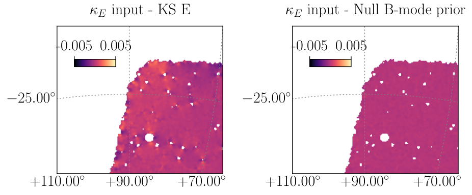
To demonstrate the effects of the mask and missing data, we generate a mock catalogue with no shape noise. Fig. 2 shows the input true convergence map (top left), the KS E-mode reconstruction (top left), the KS residual map (bottom left), and the KS B-mode map (bottom right). The residual is defined as the difference between the input true map and the reconstructed E-mode map. In these figures the maps have been smoothed with a Gaussian kernel with for visualization.
In the noise-free case all methods other than KS (including Wiener and Glimpse) have a null B-mode prior and are thus equivalent. In this noise-free limit, the noise covariance becomes a binary matrix (for the mask) and the signal factors can divide out (although our code implementations of Wiener and Glimpse would not be able to deal with this zero limit in practice). The noise-free result is therefore the same for the null B-mode prior method, the Wiener filter, and Glimpse.
From the KS residual map (bottom left), where the residual is between the KS idealised case with no shape noise and the truth, we recover most of the features of the input convergence map, except for the part of the map close to the edges of the DES footprint. As discussed in Sec. 3, the KS reconstruction is susceptible to mask effects in the case of partial sky coverage, resulting in a non-zero residual map and spurious B-modes (i.e. E-mode leakage). The amplitude of the residual map is strongly reduced when a null B-mode prior is applied, as shown in Fig. 3. We can also quantify the effect of the null B-mode prior by measuring the power spectra of the recovered maps. In Fig. 4 we compare the power spectra of the KS and null B-mode prior maps with the input convergence map power spectrum. The maps have not been smoothed in this comparison. We use the HEALPix routine anafast to estimate the power spectra of our maps. The power spectra are binned in 20 bins between and . Fig. 4 clearly shows that the KS method underpredicts the power spectrum at large scales, due to mask effects and E-mode leakage. The null B-mode prior, on the contrary, better recovers the power spectrum at all scales. This holds in the case the spurious B-modes are caused only by mask and edge effects. As all the methods other than KS include a null B-mode prior, these methods are less susceptible to mask effects.
5.2 Reconstruction from realistic mock data
Fig. 5 shows the reconstructed maps from the simulated realistic noisy shear catalogue using the four methods for comparison. Again, the KS and the null-B-mode reconstruction have been smoothed at . The Glimpse reconstruction uses a sparsity parameter of (discussed below). Recall that all the map making methods take into account the noise covariance matrix of the data, thereby characterising the noise amplitude and distribution across the observed area. As a result, all methods naturally take into account inhomogeneities in the noise properties across the DES Y3 footprint.
The KS E-mode map is now noticeably degraded compared to the noise-free example (Fig. 2). Though the most significant features of the input convergence field can still be spotted by eye, a number of noise-induced small-scale peaks dominate the reconstructed map. The null B-mode prior method map looks similar to the KS E mode map, whereas the impact of noise is reduced in the case of the other methods, due to their signal priors in the map inference process. In particular, the sparsity prior adopted by the Glimpse method suppresses the noise enhancing peaky features, which are assumed to be the result of a superposition of spherically symmetric dark matter haloes (a feature that can be noted in the zoomed-in portion of the Glimpse map). The noise is also suppressed in the case of the Wiener filter reconstruction, although the map shows fewer peak features compared to the Glimpse map. The Wiener method has a prior distribution for which the convergence field is a realization of Gaussian random field, and therefore it is better suited to recover the large-scale structures in the map that have been less affected by non-linear structure collapse.
5.3 Pearson correlation coefficient
The first statistic we examine is the Pearson correlation coefficient, which quantifies the correlation between the true convergence from simulation and the reconstructed convergence from the simulated mock data catalogue. The Pearson coefficient also reveals the ability of one method to preserve the phases of the convergence field, as it would assume low values if phases were not preserved. The Pearson correlation coefficient, defined for two convergence fields and , is given by
| (35) |
where is the sample covariance estimated using pixel values of and .
In this case, we compute the Pearson correlation coefficient between the true simulated convergence map and the reconstructed E-mode convergence map. The results are shown in Fig. 6. In general, the closer to unity the Pearson coefficient value, the better the reconstruction.
For KS and the null B-mode prior methods the smoothing parameter of the Gaussian kernel was varied, while for Glimpse we varied the sparsity parameter . Recall that in our implementation of the null B-mode prior method the map is recursively smoothed at every iteration of the algorithm, so that the final map is slightly smoother than if it were smoothed only at the end of the iterative procedure. This means that in practice a given value of the smoothing parameter for the null B-mode prior method should be compared to a slightly larger value for the KS method.
The effect of the tuning parameter for the null B-mode prior method is similar to KS, although the former method performs slightly better at small smoothing parameter values. The KS and null B-mode prior methods maximise the Pearson coefficient at of smoothing respectively. This is due the small angular scales being shape noise dominated, with corresponding to the scale where the amplitude of shape noise is comparable to the amplitude of the signal. One can interpret this as the smoothing up to removing more small-scale noise-induced spurious structures than true signal. A different shape noise contribution (or, equivalently, a different data set) would change this scale; in the limit of no shape noise, the optimal scale would be the smallest scale allowed by the pixelization scheme. The null B-mode prior method performs slightly better than KS at small because of the extra regularization (i.e. smoothing) performed at every step of the iterative algorithm; this further suppresses noise, improving the Pearson coefficient at small scales.
For Glimpse, the level of suppression of the shape noise is controlled by the sparsity coefficient , for which we found to optimize the Pearson correlation coefficient. The Wiener filter has no free parameters in our implementation provided the fiducial power spectrum is assumed. Both Glimpse and the Wiener filter outperform standard KS and null B-mode prior methods, delivering a higher Pearson coefficient.
5.4 RMSE
The second statistic we examine is the root-mean-square error (RMSE) of the residuals, defined to be
| (36) |
where is the number of pixels and is the difference between the reconstructed map and the true map in pixel . Again, we only consider E-mode maps and maps recovered from noisy estimates of the shear field. The results are shown in Fig. 6. In general, the closer to zero the RMSE, the better the reconstruction. The RMSE reveals the ability of one method to preserve the phases and the amplitude of the convergence field.
The results from this test match those from the Pearson coefficient test. The null B-mode prior method shows a similar trend to the KS method, although it is characterized by a smaller RMSE at small scales. The Glimpse and Wiener methods perform better (i.e. the RMSE is closer to zero) than standard KS and the null B-mode prior methods.
For KS and the null B-mode prior methods the RMSE is reduced strongly with smoothing, indicating that the variance at small scales is completely dominated by shape noise, reaching a minimum after smoothing the reconstructed maps at . We note that the minimum of the RMSE signal and the maximum of the Pearson coefficient for these two maps are at a similar smoothing parameter value (even though the value does not need to be exactly the same). For these two methods, the RMSE should converge at very large smoothing parameter values (larger than those showed here) to the RMSE of the original field, as the reconstructed map signal goes to zero. Similar to the Pearson coefficient case, the null B-mode prior method has a smaller RMSE compared to KS at small scales, due to the extra noise suppression of the algorithm.
The Glimpse and Wiener methods have a significantly smaller RMSE compared to KS, meaning the reconstructed Glimpse and Wiener maps map is more accurate than KS on the pixel level. For Glimpse the minimum RMSE is reached for a sparsity parameter , the same value that maximises the Pearson coefficient.
5.5 Power spectra
We now examine, for each method, the power spectrum of the residual map (defined to be the difference between the reconstructed map and the input convergence map) and the power spectrum of the reconstructed map. Recall that the reconstruction is a maximum a posteriori estimate, so the power spectrum of is not expected to match the power spectrum of the underlying field (Sec. 3.6).
The differences between power spectra highlight the effect of different priors on the maximum a posteriori reconstruction, whereas the residual map power spectra show at which scales the recovered maps are most similar to the input convergence field. For these tests, we use the maps recovered from a noisy version of the shear field. We use the HEALPix routine anafast to estimate the power spectra of our maps. The power spectra are binned in 20 bins between and . For the KS and the null B-modes prior methods, we considered the maps with smoothing; for the Glimpse method, we considered the map obtained with sparsity parameter .
The left panel of Fig. 7 shows the power spectra of the maps compared to the power spectrum of the input convergence field. There is a clear signal suppression at small scales and high multipoles; this is a consequence of the priors implemented by the different methods to reduce the impact of noise (which dominates the small-scale regime). The KS and the null B-modes prior methods show similar behaviour, as they implement similar priors; however, the null B-mode prior method suppresses the small-scale signal slightly more compared to KS. In general, none of the methods reproduce the correct amplitude of the input theory power spectra; this is to be expected with point-estimate reconstructions of the map (Sec. 3.6).
The right panel of Fig. 7 shows the power spectra of the residual maps. At large scales the Wiener map shows the smallest amplitude, indicating that it performs best at reproducing the large-scale pattern of the convergence field. For Wiener and Glimpse maps, the residuals steadily increase at larger multipoles; indeed, none of the methods is able to recover the small-scale information. Besides this main trend, the KS and null B-mode prior maps also show an increment in the residual map power spectrum around . The smoothing prior is not able to reduce the impact of shape noise at these scales, causing the residual map power spectrum to increase substantially. This shows that the Wiener and Glimpse methods are indeed better than the KS and null B-mode prior methods at recovering intermediate scales.
5.6 Convergence one-point distribution and recovery of the input convergence pixel values
In Fig. 8 we show the one-point distribution function (PDF) of the convergence field. For KS and the null B-mode prior reconstructions we considered maps with smoothing, and we used for Glimpse.
The PDFs of the pixel values of the reconstructed maps are not identical to those of the input. This is expected. As all reconstructions are a maximum a posteriori estimate of the underlying convergence field, the variance (and possibly higher-order moments) of the reconstructed map will be suppressed. The asymmetric distributions are a sign that the recovered map is not dominated by noise, whose PDF is completely symmetric.
We also show in Fig. 9 density plots illustrating the relation between the values of the pixels of the recovered maps and those of the input convergence map. For a perfect reconstruction, the density plots would look like a straight, diagonal line (the black line in the Figure). In general, it can be noted that the values of the pixels of the recovered maps scatter more around zero than the values of the pixels of the input map. This is a consequence of the noise; however, as already noted in Fig. 8, the density plots not being perfectly symmetric means that the maps are not dominated by noise. Generally, pixels with negative (positive) values in the recovered maps are also associated to the ones with negative (positive) values in the input convergence map, although with a large scatter. The scatter is larger for pixels with positive values, due to the long positive tail of the convergence PDF.
The density plots for the Wiener filter and Glimpse maps are tighter, whereas KS and null B-mode prior method show a larger scatter. The density plots convey the same information encoded by the RMSE: a higher (lower) RMSE value is associated to a tighter (broader) density plot around the black diagonal line in Fig. 9.
6 Application to data
6.1 Map reconstruction
In this section we present the reconstructed mass maps using DES Y3 weak lensing data. We show only maps created using the full catalogue. We also created maps for the four tomographic bins; they are not shown here, but they will be made publicly available following publication at https://des.ncsa.illinois.edu/releases.
Fig. 10 shows the four maps obtained with the KS, null B-mode prior, Wiener filter and Glimpse methods, obtained from the METACALIBRATION catalogue. We recall that these maps have been obtained applying the METACALIBRATION response correction and the inverse variance weights, as explained in Sec. 1. The maps obtained with the different methods visually show the same differences as the ones obtained in simulations (Fig. 5), with the Wiener and Glimpse maps particularly suppressing the noise thanks to their priors.


6.2 Systematic error tests
We perform a number of tests on the recovered maps. We first test if any spurious correlation exists between our maps and quantities that are not expected to correlate with the convergence maps. The shear catalogue used to produce the mass maps have been largely tested in Gatti et al. 2021, but the potential correlation between convergence maps and systematic errors was not investigated there. We therefore consider a number of catalogue and observational properties as potential systematic errors, in a fashion similar to what was done in Gatti et al. 2021. In particular, we consider the two components of the point-spread-function (PSF) ellipticity at the galaxy position (, ), their E and B-modes maps (, ), and the size of the PSF (). As observing condition properties, we consider mean air-mass, mean brightness, mean magnitude limit (depth), mean exposure time, and mean seeing (all in the i-band).
A few maps were considered in the shear catalogue tests and so are excluded here. For example, we do not include the signal-to-noise ratio maps among the systematic maps, as we actually expect to measure a signal (indeed, overdense regions of the sky should be populated by red elliptical galaxies with high signal-to-noise). Similarly, we expect (and measure) at high significance a correlation between galaxy colours and our mass maps.

We follow Chang et al. 2018 and create (using mean-subtracted values) a systematic map for each of the systematic errors. We first assume a linear dependence between the convergence maps and the systematic maps:
| (37) |
We fit all the pixel values of the convergence maps assuming such a linear relationship with the systematic maps. We show the measured coefficient for each of these systematic maps in the left panel of Fig. 11. Errors are estimated using jackknife errors. We do not find any particularly significant correlation; individually, the coefficients are measured with a significance smaller than . The overall of the null hypothesis (considering the correlations among the 10 systematic maps considered here) is 6, 12, 10, and 17 for 10 , for KS, null B-mode prior, Wiener, and Glimpse respectively, indicating compatibility with no significant dependence on systematic errors. We also compute the Pearson coefficient between the convergence maps and the systematic maps; results are shown in the right panel of Fig. 11 (note that in the same Figure we also show the Pearson coefficient with redMaPPer clusters, discussed in the next section). The main difference with the linear fit is that the Pearson coefficient does not assume a priori any relation between the convergence maps and systematic maps. Again, we do not find any strong evidence of systematic contamination, with the of the null hypothesis being 5, 5, 7, and 10 for 10 , for KS, null B-mode prior, Wiener, and Glimpse respectively.
6.3 Structures in the reconstructed maps
6.3.1 Galaxy cluster distribution
For obvious reasons the true convergence map is not available in data; nevertheless we can check that the reconstructed mass maps probe the foreground matter density field by correlating them with a sample of other tracers. For visualization purposes, we show in Fig. 12 the Glimpse map with a few redMaPPer clusters superimposed.
From Fig. 12 we can see that clusters tend to populate the densest regions in the reconstructed convergence map and avoid the regions with negative convergence signal.
We also report in Fig. 11 the Pearson coefficient between the maps and the effective richness of redMaPPer clusters at . In particular, we follow Jeffrey et al. 2018b and define an effective lensed cluster richness :
| (38) |
where is the redMaPPer cluster richness, is the scale factor evaluated at the comoving distance to a given cluster , and is the lensing efficiency, defined as , with the redshift distribution of the source galaxies used to create the mass maps as a function of comoving density. The effective richness is then normalised to the mean of the effective richness of all clusters considered. For all the maps, the measured Pearson coefficient shown in Fig. 11 is significantly larger than 0, showing how the recovered maps successfully trace the foreground matter density field. Again, we use parameter value arcmin for the KS and the null B-mode prior reconstruction and for Glimpse by default. For the redMaPPer result in the right panel of Fig. 11, we also plot arcmin and (the triangular figure markers), which were shown to improve the correlation for these maps.
6.3.2 Cosmic void imprints
Cosmic voids are an increasingly favoured cosmic probe and have now already been successfully used to extract cosmological information (Pisani et al. 2019, for a recent overview see). We expect these large lower-density regions in the cosmic web to display a typical imprinting in the convergence signal when cross-correlated with weak lensing mass maps (Chang et al. 2018, for previous results from DES Y1 data see).
We create a catalogue of so-called ‘2D voids’ (Sánchez et al. 2017) from the DES Y3 redMaGiC (Rozo et al. 2016) photometric redshift data set by searching for projected underdensities in tomographic slices of the galaxy catalogue. On average, these tunnel-like voids correspond to density minima that are compensated by an overdense zone in their surroundings. With this simple approach, we detect voids in the DES Y3 data set, which are larger on average, although also less underdense, than most voids from other void finders (Fang et al. 2019, see e.g.). They certainly are useful tools in void lensing studies (Davies et al. 2018) and they have been widely used in previous DES analyses (Vielzeuf et al. 2021; Kovács et al. 2017; Kovács et al. 2019; Fang et al. 2019, see e.g.).
The lensing imprint of typical individual voids is expected to be undetectable (Amendola et al. 1999). Therefore, after selecting our void sample, we follow a stacking method to measure the mean signal of all voids (Vielzeuf et al. 2021, see e.g.). Knowing the angular size of voids, we re-scale the local mass map patches around the void centres. In such re-scaled units, we then extract convergence patches five times the void radius, stack them to increase signal-to-noise, and measure radial profiles from the average patch. Without a large set of simulations to estimate covariance of the void profile statistic, we estimate uncertainty using a void-by-void jackknife method (Sánchez et al. 2017, see e.g.). We then correct these re-sampling based uncertainties with reference to previous DES Y1 void analysis results that used more accurate Monte Carlo simulations (Vielzeuf et al. 2021).
Fig. 13 shows the measured profiles using the DES voids. As anticipated, we detect a negative convergence signal within the void radius () and a surrounding ring () of positive convergence signal (due to compensating mass around voids). We note that different mass map versions show consistent signals (within the quoted uncertainties). While these void lensing results remain open to much further quantitative work, there is certainly clear detection of correlations between underdensities of galaxies and matter; this will motivate further studies using DES Y3. We finally remark that the typical convergence signal associated with local underdensities can be affected by the void definition and selection. We explore alternative void samples extracted from DES Y3 data in Appendix B.
6.3.3 Line-of-sight underdensities
Posing a slightly different question, we also examine the distribution of galaxies in a line-of-sight aligned with the most negative fluctuations in the DES Y3 mass maps. We call these voids in lensing maps or voles (Davies et al. 2018, see e.g.). We use a slightly modified version of the 2D void finder algorithm to identify them in the DES mass maps. We apply a Gaussian smoothing of 2 deg in order to intentionally select relatively deep and extended voles.
Following the previous DES Year 1 (Y1) analyses (Chang et al. 2018), the redMaGiC galaxy position catalogue is projected into two-dimensional slices of 100 along the line-of-sight. This thickness corresponds to the approximate photo- errors of the redMaGiC galaxies that allows the robust identification of voids (see Sánchez et al. 2017, for details). At redshifts , galaxy density contrasts are measured in 15 tomographic slices aligned with voles. Galaxies are counted within an aperture of 2 deg of the void centre, which approximately corresponds to the full angular size of voles. The measured density contrasts at the different redshifts are used to reconstruct the radial density profile aligned with the given vole. Fig. 14 shows the line-of-sight galaxy density aligned with a significant vole at in the KS map.
We find an extended underdensity that is consistent with a super-void with radius (assuming simple Gaussian void profiles as in Finelli et al. 2016). This super-void, similar to the biggest underdensity found in the preceding DES Y1 analysis (Chang et al. 2018), will have smaller-scale substructures that are inaccessible using redMaGiC photometric redshift data. Nevertheless, such a super-void is comparable to the largest known underdensities in the local Universe, and these objects are of great interest in cosmology (Shimakawa et al. 2021, see e.g.). Their integrated Sachs-Wolfe imprint has already been studied using DES Y3 data to probe dark energy (Kovács et al. 2019, for details see).
7 Summary
In this work we constructed weak lensing convergence maps (‘mass maps’) from the DES Y3 data set using four reconstruction methods. The first method considered is the direct inversion of the shear field, also known as the Kaiser-Squires method, followed by a smoothing of small angular scales. The second method uses a prior on the B-modes of the map, imposing that the reconstructed convergence field must be purely an E-mode map (null B-mode prior); this method also includes smoothing at small scales. The third method, the Wiener filter, uses a Gaussian prior distribution for the underlying convergence field. Lastly, the Glimpse method implements a sparsity prior in wavelet (starlet) space, which can be interpreted as a physical model where the matter field is composed of a superposition of spherically symmetric haloes.
All methods are implemented on the sphere to accommodate the large sky coverage of the DES Y3 footprint. We compared the different methods using simulations that are closely matched to the DES Y3 data. We quantified the performance of the methods at the map level using a number of different summary statistics: the Pearson coefficient with the ‘true’ simulated convergence map, the root-mean-square error (RMSE) of the residual maps, the power spectra of the mass maps and residual maps, and the 1-point distribution function (PDF) of the mass maps.
The tests performed suggested that using our physically-motivated priors to recover the convergence field from a noisy realization of the shear field generally improves some aspects of the reconstruction. In particular, null B-mode, Wiener, and Glimpse delivered larger values of the Pearson coefficient and smaller values of the RMSE compared to the standard KS method, indicating that their use of physically-motivated informative priors significantly improve the accuracy of the reconstruction. We furthermore showed that a null B-mode prior mitigates the troublesome effects of masks and missing data. We also note how the choice of the prior can make the comparison of certain statistics with theoretical predictions non-trivial when taking the maximum a posteriori result as a point estimate , rather than evaluating the full posterior distribution ). Even if the effect of the prior cannot be easily modelled for a given theoretical summary statistic for cosmological inference, a forward modelling framework can be implemented that compares observed and simulated summary statistics.
We have presented the official DES Y3 mass maps, obtained with the four different methods, and assessed their robustness against a number of systematic error maps representing catalogue properties and observing conditions. This recovered mass map, of which the dominant mass contribution is dark matter, covers the largest sky fraction of any galaxy weak lensing map of the late Universe.
We emphasize that the choice of the particular mass map method depends on the goals and details of the science application. Science applications of these DES Y3 mass maps are expected in future work.
Acknowledgments
Funding for the DES Projects has been provided by the U.S. Department of Energy, the U.S. National Science Foundation, the Ministry of Science and Education of Spain, the Science and Technology Facilities Council of the United Kingdom, the Higher Education Funding Council for England, the National Center for Supercomputing Applications at the University of Illinois at Urbana-Champaign, the Kavli Institute of Cosmological Physics at the University of Chicago, the Center for Cosmology and Astro-Particle Physics at the Ohio State University, the Mitchell Institute for Fundamental Physics and Astronomy at Texas A&M University, Financiadora de Estudos e Projetos, Fundação Carlos Chagas Filho de Amparo à Pesquisa do Estado do Rio de Janeiro, Conselho Nacional de Desenvolvimento Científico e Tecnológico and the Ministério da Ciência, Tecnologia e Inovação, the Deutsche Forschungsgemeinschaft and the Collaborating Institutions in the Dark Energy Survey.
The Collaborating Institutions are Argonne National Laboratory, the University of California at Santa Cruz, the University of Cambridge, Centro de Investigaciones Energéticas, Medioambientales y Tecnológicas-Madrid, the University of Chicago, University College London, the DES-Brazil Consortium, the University of Edinburgh, the Eidgenössische Technische Hochschule (ETH) Zürich, Fermi National Accelerator Laboratory, the University of Illinois at Urbana-Champaign, the Institut de Ciències de l’Espai (IEEC/CSIC), the Institut de Física d’Altes Energies, Lawrence Berkeley National Laboratory, the Ludwig-Maximilians Universität München and the associated Excellence Cluster Universe, the University of Michigan, NFS’s NOIRLab, the University of Nottingham, The Ohio State University, the University of Pennsylvania, the University of Portsmouth, SLAC National Accelerator Laboratory, Stanford University, the University of Sussex, Texas A&M University, and the OzDES Membership Consortium.
Based in part on observations at Cerro Tololo Inter-American Observatory at NSF’s NOIRLab (NOIRLab Prop. ID 2012B-0001; PI: J. Frieman), which is managed by the Association of Universities for Research in Astronomy (AURA) under a cooperative agreement with the National Science Foundation.
The DES data management system is supported by the National Science Foundation under Grant Numbers AST-1138766 and AST-1536171. The DES participants from Spanish institutions are partially supported by MICINN under grants ESP2017-89838, PGC2018-094773, PGC2018-102021, SEV-2016-0588, SEV-2016-0597, and MDM-2015-0509, some of which include ERDF funds from the European Union. IFAE is partially funded by the CERCA program of the Generalitat de Catalunya. Research leading to these results has received funding from the European Research Council under the European Union’s Seventh Framework Program (FP7/2007-2013) including ERC grant agreements 240672, 291329, and 306478. We acknowledge support from the Brazilian Instituto Nacional de Ciência e Tecnologia (INCT) do e-Universo (CNPq grant 465376/2014-2).
This manuscript has been authored by Fermi Research Alliance, LLC under Contract No. DE-AC02-07CH11359 with the U.S. Department of Energy, Office of Science, Office of High Energy Physics.
NJ has been supported by funding from l’Ecole Normale Supérieure, Paris. OL and NJ acknowledge support from a European Research Council Advanced Grant TESTDE (FP7/291329) and STFC Consolidated Grants ST/M001334/1 and ST/R000476/1. AK has been supported by a Juan de la Cierva fellowship from MINECO with project number IJC2018-037730-I, and funding for this project was also available in part through SEV-2015-0548 and AYA2017-89891-P. Cosmic voids computational work has been performed on the UK SCIAMA High Performance Computing cluster supported by the ICG, SEPNet and the University of Portsmouth.
Data availability
The full metacalibration catalogue and mass maps will be made publicly available following publication, at https://des.ncsa.illinois.edu.
References
- Abbott et al. (2018) Abbott T. M. C., et al., 2018, ApJS, 239, 18
- Ajani et al. (2020) Ajani V., Peel A., Pettorino V., Starck J.-L., Li Z., Liu J., 2020, Phys. Rev. D, 102, 103531
- Alonso et al. (2019) Alonso D., Sanchez J., Slosar A., 2019, MNRAS, 484, 4127–4151
- Alsing et al. (2017) Alsing J., Heavens A., Jaffe A. H., 2017, MNRAS, 466, 3272
- Amendola et al. (1999) Amendola L., Frieman J. A., Waga I., 1999, MNRAS, 309, 465
- Asgari et al. (2019) Asgari M., et al., 2019, A&A, 624, A134
- Bartelmann & Schneider (2001) Bartelmann M., Schneider P., 2001, Phys. Rep., 340, 291
- Blazek et al. (2019) Blazek J. A., MacCrann N., Troxel M., Fang X., 2019, Physical Review D, 100, 103506
- Castro et al. (2005) Castro P. G., Heavens A. F., Kitching T. D., 2005, Phys. Rev. D, 72, 023516
- Cautun et al. (2016) Cautun M., Cai Y.-C., Frenk C. S., 2016, Monthly Notices of the Royal Astronomical Society, 457, 2540–2553
- Chang et al. (2015) Chang C., et al., 2015, Phys. Rev. Lett., 115, 051301
- Chang et al. (2018) Chang C., et al., 2018, MNRAS, 475, 3165
- Combettes & Wajs (2005) Combettes P. L., Wajs V. R., 2005, Multiscale Modeling & Simulation, 4, 1168
- Crocce et al. (2006) Crocce M., Pueblas S., Scoccimarro R., 2006, MNRAS, 373, 369
- Dark Energy Survey Collaboration et al. (2016) Dark Energy Survey Collaboration et al., 2016, MNRAS, 460, 1270
- Davies et al. (2018) Davies C. T., Cautun M., Li B., 2018, MNRAS, 480, L101
- Dietrich & Hartlap (2010) Dietrich J. P., Hartlap J., 2010, MNRAS, 402, 1049
- Elsner & Wandelt (2013) Elsner F., Wandelt B. D., 2013, A&A, 549, A111
- Fang et al. (2019) Fang Y., et al., 2019, MNRAS, 490, 3573
- Finelli et al. (2016) Finelli F., García-Bellido J., Kovács A., Paci F., Szapudi I., 2016, MNRAS, 455, 1246
- Flaugher et al. (2015) Flaugher B., et al., 2015, AJ, 150, 150
- Fluri et al. (2018) Fluri J., Kacprzak T., Refregier A., Amara A., Lucchi A., Hofmann T., 2018, Phys. Rev. D, 98, 123518
- Fluri et al. (2019) Fluri J., Kacprzak T., Lucchi A., Refregier A., Amara A., Hofmann T., Schneider A., 2019, Phys. Rev. D, 100, 063514
- Fu et al. (2014) Fu L., et al., 2014, MNRAS, 441, 2725
- Gatti et al. (2020a) Gatti M., Giannini G., et al., 2020a, arXiv e-prints, p. arXiv:2012.08569
- Gatti et al. (2020b) Gatti M., et al., 2020b, MNRAS, 498, 4060
- Gatti et al. (2021) Gatti M., Sheldon E., et al., 2021, Mon. Not. Roy. Astron. Soc., 504, 4312
- Górski et al. (2005) Górski K. M., Hivon E., Banday A. J., Wandelt B. D., Hansen F. K., Reinecke M., Bartelmann M., 2005, ApJ, 622, 759
- Hamana et al. (2015) Hamana T., Sakurai J., Koike M., Miller L., 2015, PASJ, 67, 34
- Hamana et al. (2020) Hamana T., et al., 2020, PASJ, 72, 16
- Hamaus et al. (2020) Hamaus N., Pisani A., Choi J.-A., Lavaux G., Wandelt B. D., Weller J., 2020, J. Cosmology Astropart. Phys., 2020, 023
- Higson et al. (2019) Higson E., Handley W., Hobson M., Lasenby A., 2019, MNRAS, 483, 4828
- Hikage et al. (2019) Hikage C., et al., 2019, PASJ, 71, 43
- Hildebrandt et al. (2017) Hildebrandt H., et al., 2017, MNRAS, 465, 1454
- Hinshaw et al. (2013) Hinshaw G., et al., 2013, ApJS, 208, 19
- Huff & Mandelbaum (2017) Huff E., Mandelbaum R., 2017, preprint (arXiv:1702.02600)
- Jasche & Lavaux (2015) Jasche J., Lavaux G., 2015, MNRAS, 447, 1204
- Jeffrey et al. (2018a) Jeffrey N., Heavens A. F., Fortio P. D., 2018a, Astronomy and Computing, 25, 230
- Jeffrey et al. (2018b) Jeffrey N., et al., 2018b, MNRAS, 479, 2871
- Jeffrey et al. (2020) Jeffrey N., Lanusse F., Lahav O., Starck J.-L., 2020, MNRAS, 492, 5023
- Jeffrey et al. (2021) Jeffrey N., Alsing J., Lanusse F., 2021, MNRAS, 501, 954
- Kacprzak et al. (2016) Kacprzak T., et al., 2016, MNRAS, 463, 3653
- Kaiser & Squires (1993) Kaiser N., Squires G., 1993, ApJ, 404, 441
- Kodi Ramanah et al. (2019) Kodi Ramanah D., Lavaux G., Wandelt B. D., 2019, MNRAS, 490, 947
- Kovács et al. (2017) Kovács A., et al., 2017, MNRAS, 465, 4166
- Kovács et al. (2019) Kovács A., et al., 2019, MNRAS, 484, 5267
- Kratochvil et al. (2010) Kratochvil J. M., Haiman Z., May M., 2010, Phys. Rev. D, 81, 043519
- Kratochvil et al. (2012) Kratochvil J. M., Lim E. A., Wang S., Haiman Z., May M., Huffenberger K., 2012, Phys. Rev. D, 85, 103513
- Krause & Hirata (2010) Krause E., Hirata C. M., 2010, A&A, 523, A28
- Lanusse et al. (2016) Lanusse F., Starck J. L., Leonard A., Pires S., 2016, A&A, 591, A2
- Liu et al. (2015) Liu J., Petri A., Haiman Z., Hui L., Kratochvil J. M., May M., 2015, Phys. Rev. D, 91, 063507
- MacCrann et al. (2020) MacCrann N., et al., 2020, Submitted to MNRAS
- Mandelbaum (2018a) Mandelbaum R., 2018a, ARA&A, 56, 393
- Mandelbaum (2018b) Mandelbaum R., 2018b, ARA&A, 56, 393
- Marshall et al. (2002) Marshall P. J., Hobson M. P., Gull S. F., Bridle S. L., 2002, MNRAS, 335, 1037
- Martinet et al. (2018) Martinet N., et al., 2018, MNRAS, 474, 712
- Mawdsley et al. (2020) Mawdsley B., et al., 2020, MNRAS, 493, 5662
- Morganson et al. (2018) Morganson E., et al., 2018, PASP, 130, 074501
- Muir et al. (2020) Muir J., et al., 2020, MNRAS, 494, 4454
- Myles et al. (2020) Myles J., Alarcon A., et al., 2020, arXiv e-prints, p. arXiv:2012.08566
- Nadathur & Crittenden (2016) Nadathur S., Crittenden R., 2016, ApJ, 830, L19
- Nadathur et al. (2017) Nadathur S., Hotchkiss S., Crittenden R., 2017, MNRAS, 467, 4067
- Nadathur et al. (2018) Nadathur S., Carter P., Percival W. J., 2018, MNRAS, 482, 2459–2470
- Nadathur et al. (2019) Nadathur S., Carter P. M., Percival W. J., Winther H. A., Bautista J. E., 2019, Physical Review D, 100
- Navarro et al. (1996) Navarro J. F., Frenk C. S., White S. D. M., 1996, ApJ, 462, 563
- Neyrinck (2008) Neyrinck M. C., 2008, MNRAS, 386, 2101
- Oguri et al. (2018) Oguri M., et al., 2018, PASJ, 70, S26
- Parroni et al. (2020) Parroni C., Cardone V. F., Maoli R., Scaramella R., 2020, A&A, 633, A71
- Peel et al. (2018) Peel A., Pettorino V., Giocoli C., Starck J.-L., Baldi M., 2018, A&A, 619, A38
- Petri et al. (2015) Petri A., Liu J., Haiman Z., May M., Hui L., Kratochvil J. M., 2015, Phys. Rev. D, 91, 103511
- Pisani et al. (2019) Pisani A., et al., 2019, BAAS, 51, 40
- Pollina et al. (2019) Pollina G., et al., 2019, Monthly Notices of the Royal Astronomical Society, 487, 2836–2852
- Price et al. (2019) Price M. A., Cai X., McEwen J. D., Pereyra M., Kitching T. D., 2019, MNRAS, 492, 394
- Price et al. (2021) Price M. A., McEwen J. D., Pratley L., Kitching T. D., 2021, MNRAS, 500, 5436
- Raghunathan et al. (2020) Raghunathan S., Nadathur S., Sherwin B. D., Whitehorn N., 2020, ApJ, 890, 168
- Ribli et al. (2019) Ribli D., Pataki B. Á., Csabai I., 2019, Nature Astronomy, 3, 93
- Rozo et al. (2016) Rozo E., et al., 2016, MNRAS, 461, 1431–1450
- Samuroff et al. (2019) Samuroff S., et al., 2019, MNRAS, 489, 5453
- Sánchez et al. (2017) Sánchez C., et al., 2017, MNRAS, 465, 746
- Sánchez et al. (2020) Sánchez C., Prat J., et al., 2020, To be submitted to MNRAS
- Seitz & Schneider (1997) Seitz C., Schneider P., 1997, A&A, 318, 687
- Semboloni et al. (2011) Semboloni E., Schrabback T., van Waerbeke L., Vafaei S., Hartlap J., Hilbert S., 2011, MNRAS, 410, 143
- Sevilla-Noarbe et al. (2020) Sevilla-Noarbe I., et al., 2020, arXiv e-prints, p. arXiv:2011.03407
- Sevilla et al. (2011) Sevilla I., et al., 2011, in Meeting of the APS Division of Particles and Fields. (arXiv:1109.6741)
- Shan et al. (2018) Shan H., et al., 2018, MNRAS, 474, 1116
- Sheldon & Huff (2017) Sheldon E. S., Huff E. M., 2017, ApJ, 841, 24
- Sheldon et al. (2020) Sheldon E. S., Becker M. R., MacCrann N., Jarvis M., 2020, ApJ, 902, 138
- Shimakawa et al. (2021) Shimakawa R., et al., 2021, arXiv e-prints, p. arXiv:2103.04291
- Shirasaki et al. (2019) Shirasaki M., Yoshida N., Ikeda S., 2019, Phys. Rev. D, 100, 043527
- Springel (2005) Springel V., 2005, MNRAS, 364, 1105
- Starck et al. (2007) Starck J.-L., Fadili J., Murtagh F., 2007, IEEE transactions on image processing, 16, 297
- Starck et al. (2015) Starck J.-L., Murtagh F., Fadili J., 2015, Sparse Image and Signal Processing: Wavelets and Related Geometric Multiscale Analysis, Second Edition, 2 edn. Cambridge University Press, doi:10.1017/CBO9781316104514
- Starck et al. (2021) Starck J. L., Themelis K. E., Jeffrey N., Peel A., Lanusse F., 2021, arXiv e-prints, p. arXiv:2102.04127
- Sutter et al. (2015) Sutter P. M., et al., 2015, Astronomy and Computing, 9, 1
- Takada & Jain (2003) Takada M., Jain B., 2003, MNRAS, 344, 857
- Takada & Jain (2004) Takada M., Jain B., 2004, MNRAS, 348, 897
- Takahashi et al. (2012) Takahashi R., Sato M., Nishimichi T., Taruya A., Oguri M., 2012, ApJ, 761, 152
- Takahashi et al. (2017) Takahashi R., Hamana T., Shirasaki M., Namikawa T., Nishimichi T., Osato K., Shiroyama K., 2017, ApJ, 850, 24
- Troxel et al. (2018) Troxel M. A., et al., 2018, Phys. Rev. D, 98, 043528
- Van Waerbeke et al. (2013) Van Waerbeke L., et al., 2013, MNRAS, 433, 3373
- Vicinanza et al. (2016) Vicinanza M., Cardone V. F., Maoli R., Scaramella R., Er X., 2016, preprint (arXiv:1606.03892)
- Vicinanza et al. (2018) Vicinanza M., Cardone V. F., Maoli R., Scaramella R., Er X., 2018, Phys. Rev. D, 97, 023519
- Vicinanza et al. (2019) Vicinanza M., Cardone V. F., Maoli R., Scaramella R., Er X., Tereno I., 2019, Phys. Rev. D, 99, 043534
- Vielzeuf et al. (2021) Vielzeuf P., et al., 2021, MNRAS, 500, 464
- Vikram et al. (2015) Vikram V., et al., 2015, Phys. Rev. D, 92, 022006
- Wallis et al. (2017) Wallis C. G. R., McEwen J. D., Kitching T. D., Leistedt B., Plouviez A., 2017, preprint (arXiv:1703.09233)
- Wandelt et al. (2004) Wandelt B. D., Larson D. L., Lakshminarayanan A., 2004, Phys. Rev. D, 70, 083511
- Wiener (1949) Wiener N., 1949, Extrapolation, interpolation, and smoothing of stationary time series. Vol. 7, MIT
- Zaroubi et al. (1995) Zaroubi S., Hoffman Y., Fisher K. B., Lahav O., 1995, ApJ, 449, 446
- Zuntz et al. (2018) Zuntz J., Sheldon E., et al., 2018, MNRAS, 481, 1149
Appendix A Author Affiliations
1 Laboratoire de Physique de l’Ecole Normale Supérieure, ENS, Université PSL, CNRS, Sorbonne Université, Université de Paris, Paris, France
2 Department of Physics & Astronomy, University College London, Gower Street, London, WC1E 6BT, UK
3 Institut de Física d’Altes Energies (IFAE), The Barcelona Institute of Science and Technology, Campus UAB, 08193 Bellaterra (Barcelona) Spain
4 Department of Physics and Astronomy, University of Pennsylvania, Philadelphia, PA 19104, USA
5 Department of Astronomy and Astrophysics, University of Chicago, Chicago, IL 60637, USA
6 Kavli Institute for Cosmological Physics, University of Chicago, Chicago, IL 60637, USA
7 Instituto de Astrofísica de Canarias (IAC), Calle Vía Láctea, E-38200, La Laguna, Tenerife, Spain
8 Departamento de Astrofísica, Universidad de La Laguna (ULL), E-38206, La Laguna, Tenerife, Spain
9 Universitäts-Sternwarte, Fakultät für Physik, Ludwig-Maximilians Universität München, Scheinerstr. 1, 81679 München, Germany
10 Institute of Cosmology and Gravitation, University of Portsmouth, Portsmouth, PO1 3FX, UK
11 Department of Physics, ETH Zurich, Wolfgang-Pauli-Strasse 16, CH-8093 Zurich, Switzerland
12 AIM, CEA, CNRS, Université Paris-Saclay, Université de Paris, F-91191 Gif-sur-Yvette, France
13 Argonne National Laboratory, 9700 South Cass Avenue, Lemont, IL 60439, USA
14 Kavli Institute for Particle Astrophysics & Cosmology, P. O. Box 2450, Stanford University, Stanford, CA 94305, USA
15 Physics Department, 2320 Chamberlin Hall, University of Wisconsin-Madison, 1150 University Avenue Madison, WI 53706-1390
16 Department of Physics, Carnegie Mellon University, Pittsburgh, Pennsylvania 15312, USA
17 Instituto de Astrofisica de Canarias, E-38205 La Laguna, Tenerife, Spain
18 Laboratório Interinstitucional de e-Astronomia - LIneA, Rua Gal. José Cristino 77, Rio de Janeiro, RJ - 20921-400, Brazil
19 Universidad de La Laguna, Dpto. Astrofísica, E-38206 La Laguna, Tenerife, Spain
20 Center for Astrophysical Surveys, National Center for Supercomputing Applications, 1205 West Clark St., Urbana, IL 61801, USA
21 Department of Astronomy, University of Illinois at Urbana-Champaign, 1002 W. Green Street, Urbana, IL 61801, USA
22 Department of Physics, Duke University Durham, NC 27708, USA
23 Center for Cosmology and Astro-Particle Physics, The Ohio State University, Columbus, OH 43210, USA
24 Jodrell Bank Center for Astrophysics, School of Physics and Astronomy, University of Manchester, Oxford Road, Manchester, M13 9PL, UK
25 Department of Astronomy, University of California, Berkeley, 501 Campbell Hall, Berkeley, CA 94720, USA
26 Santa Cruz Institute for Particle Physics, Santa Cruz, CA 95064, USA
27 Fermi National Accelerator Laboratory, P. O. Box 500, Batavia, IL 60510, USA
28 Department of Physics, The Ohio State University, Columbus, OH 43210, USA
29 Jet Propulsion Laboratory, California Institute of Technology, 4800 Oak Grove Dr., Pasadena, CA 91109, USA
30 Department of Physics, Stanford University, 382 Via Pueblo Mall, Stanford, CA 94305, USA
31 SLAC National Accelerator Laboratory, Menlo Park, CA 94025, USA
32 Department of Physics, University of Oxford, Denys Wilkinson Building, Keble Road, Oxford OX1 3RH, UK
33 Department of Astronomy, University of Geneva, ch. d’Écogia 16, CH-1290 Versoix, Switzerland
34 Department of Physics, University of Michigan, Ann Arbor, MI 48109, USA
35 Department of Applied Mathematics and Theoretical Physics, University of Cambridge, Cambridge CB3 0WA, UK
36 Instituto de Física Gleb Wataghin, Universidade Estadual de Campinas, 13083-859, Campinas, SP, Brazil
37 Centro de Investigaciones Energéticas, Medioambientales y Tecnológicas (CIEMAT), Madrid, Spain
38 Brookhaven National Laboratory, Bldg 510, Upton, NY 11973, USA
39 Institut d’Estudis Espacials de Catalunya (IEEC), 08034 Barcelona, Spain
40 Institute of Space Sciences (ICE, CSIC), Campus UAB, Carrer de Can Magrans, s/n, 08193 Barcelona, Spain
41 Max Planck Institute for Extraterrestrial Physics, Giessenbachstrasse, 85748 Garching, Germany
42 Institute for Astronomy, University of Edinburgh, Edinburgh EH9 3HJ, UK
43 Cerro Tololo Inter-American Observatory, NSF’s National Optical-Infrared Astronomy Research Laboratory, Casilla 603, La Serena, Chile
44 Departamento de Física Matemática, Instituto de Física, Universidade de São Paulo, CP 66318, São Paulo, SP, 05314-970, Brazil
45 Instituto de Física Teórica, Universidade Estadual Paulista, São Paulo, Brazil
46 CNRS, UMR 7095, Institut d’Astrophysique de Paris, F-75014, Paris, France
47 Sorbonne Universités, UPMC Univ Paris 06, UMR 7095, Institut d’Astrophysique de Paris, F-75014, Paris, France
48 Department of Physics and Astronomy, Pevensey Building, University of Sussex, Brighton, BN1 9QH, UK
49 University of Nottingham, School of Physics and Astronomy, Nottingham NG7 2RD, UK
50 Astronomy Unit, Department of Physics, University of Trieste, via Tiepolo 11, I-34131 Trieste, Italy
51 INAF-Osservatorio Astronomico di Trieste, via G. B. Tiepolo 11, I-34143 Trieste, Italy
52 Institute for Fundamental Physics of the Universe, Via Beirut 2, 34014 Trieste, Italy
53 Observatório Nacional, Rua Gal. José Cristino 77, Rio de Janeiro, RJ - 20921-400, Brazil
54 Department of Physics, IIT Hyderabad, Kandi, Telangana 502285, India
55 Faculty of Physics, Ludwig-Maximilians-Universität, Scheinerstr. 1, 81679 Munich, Germany
56 Institute of Theoretical Astrophysics, University of Oslo. P.O. Box 1029 Blindern, NO-0315 Oslo, Norway
57 Instituto de Fisica Teorica UAM/CSIC, Universidad Autonoma de Madrid, 28049 Madrid, Spain
58 Department of Astronomy, University of Michigan, Ann Arbor, MI 48109, USA
59 Institute of Astronomy, University of Cambridge, Madingley Road, Cambridge CB3 0HA, UK
60 Kavli Institute for Cosmology, University of Cambridge, Madingley Road, Cambridge CB3 0HA, UK
61 School of Mathematics and Physics, University of Queensland, Brisbane, QLD 4072, Australia
62 Center for Astrophysics Harvard & Smithsonian, 60 Garden Street, Cambridge, MA 02138, USA
63 George P. and Cynthia Woods Mitchell Institute for Fundamental Physics and Astronomy, and Department of Physics and Astronomy, Texas A&M University, College Station, TX 77843, USA
64 Department of Astrophysical Sciences, Princeton University, Peyton Hall, Princeton, NJ 08544, USA
65 Institució Catalana de Recerca i Estudis Avançats, E-08010 Barcelona, Spain
66 School of Physics and Astronomy, University of Southampton, Southampton, SO17 1BJ, UK
67 Computer Science and Mathematics Division, Oak Ridge National Laboratory, Oak Ridge, TN 37831
Appendix B Alternative samples of voids
We considered alternative catalogues of voids to test how the mass map imprints may depend on the void definition and selection.
VIDE33 3 https://bitbucket.org/cosmicvoids/ (Sutter et al. 2015) is a watershed void finder based on ZOBOV (Neyrinck 2008) that has been widely employed for various void studies (see e.g. Hamaus et al. 2020, and references therein). It has already been successfully used to study voids in the DES Y1 data (Pollina et al. 2019; Fang et al. 2019).
VIDE’s default centre is the volume-weighted barycentre, which does not generally coincide with the density minimum inside the void due to non-spherical void geometry. Instead, the barycentre preserves information about the void boundary. Therefore, a different kind of imprint signal is expected when correlated with convergence maps, with more pronounced positive rings rather than negative centres (Cautun et al. 2016, for a comprehensive study on the signal associated with voids see). In the DES Y3 redMaGiC data, VIDE detected voids. We then halved this catalogue using the compensation of voids to further increase and isolate the expected signal from the boundary zone, expecting to see an enhanced positive convergence imprint from these over-compensated voids.
We are also interested in detecting the most pronounced negative signals associated with a specific subclass of large and deep voids that are under-compensated. As a third option, we thus used the public44 4 https://github.com/seshnadathur/REVOLVER/ void finder algorithm REVOLVER (Nadathur et al. 2018; Nadathur et al. 2019), also based on the ZOBOV algorithm.
A proxy for the gravitational potential (and thus for the convergence field) at the positions of voids can be defined as
| (39) |
using the average galaxy density contrast and the effective spherical radius, , where the volume is the total volume of the void (Nadathur & Crittenden 2016; Nadathur et al. 2017, for further details see). Raghunathan et al. 2020 showed that different values of the parameter indicate different (CMB) lensing imprints, including signals with either positive or negative sign, aligned with the void centre55 5 REVOLVER voids may also be defined using barycentres.. Following this, we keep only of the most under-compensated voids defined by the lowest values. Leaving more detailed analyses for future work, we note that a subclass of voids with high values would also correspond to over-compensated voids such as our VIDE sample.
Fig. 15 shows the measured profiles of our REVOLVER, VIDE, and 2D void analyses given the uncertainties. As anticipated based on the differences in the nature of the voids we selected, we detected qualitatively different signals in each case:
- •
the VIDE voids show a relative depression in convergence at the void centre compared to the pronounced peak at the void boundary, matching our expectations.
- •
the REVOLVER voids we selected are associated with strong negative imprints that in fact extend far beyond the void radius, indicating surrounding voids on average.
- •
2D voids combine the advantages of the other finders. They excel in marking the actual radius of voids in the mass map profiles, with reduced central and wall amplitudes.
We thus report that all three void types we consider show consistent signals when mass maps are varied for a given void sample. We leave more detailed analysis for future work.