跳到论文正文
W Papers独立论文阅读器 arXiv:2105.13499 论文正文 计算阅读时间 · 0%
引用这篇论文根据当前论文元数据生成,正式投稿前建议核对。


License: CC BY 4.0
arXiv:2105.13499v1 [math.PR] 27 May 2021

Stein’s method and approximating the multidimensional quantum harmonic oscillator

Ian W. McKeague    Yvik Swan
Abstract

Stein’s method is used to study discrete representations of multidimensional distributions that arise as approximations of states of quantum harmonic oscillators. These representations model how quantum effects result from the interaction of finitely many classical “worlds,” with the role of sample size played by the number of worlds. Each approximation arises as the ground state of a Hamiltonian involving a particular interworld potential function. Such approximations have previously been studied for one-dimensional quantum harmonic oscillators, but the multidimensional case has remained unresolved. Our approach, framed in terms of spherical coordinates, provides the rate of convergence of the discrete approximation to the ground state in terms of Wasserstein distance. The fastest rate of convergence to the ground state is found to occur in three dimensions. This result is obtained using a discrete density approach to Stein’s method applied to the radial component of the ground state solution.

Mathematics Subject Classification (MSC2020): 60B10, 81Q05, 81Q65
Keywords: Coupling, Hamiltonian, point configurations, Stein’s method, Wasserstein distance

Author affiliations:
Ian W. McKeague: Columbia University, New York, U.S.A.
Yvik Swan: Université libre de Bruxelles, Bruxelles, Belgium.

Corresponding author: Yvik Swan

Acknowledgments. The authors thank Louis Chen, Davy Paindaveine, Erol Peköz, Gesine Reinert and Thomas Verdebout for helpful discussions.

Declarations:
Funding: The research of Ian McKeague was partially supported by National Science Foundation Grant DMS 2112938 and National Institutes of Health Grant AG062401. The research of Yvik Swan was supported by by grant CDR/OL J.0197.20 from FRS-FNRS.
Availability of data and material: provided in the Supplementary material.
Code availability: provided in the Supplementary material.

1 Introduction

The many interacting worlds (MIW) approach to quantum mechanics due to Hall et al. [9] posits a Hamiltonian for a one-dimensional harmonic oscillator of the form

H1​(𝐱,𝐩)=E⁡(𝐩)+V1​(𝐱)+U1​(𝐱),H_{1}({\bf x},{\bf p})=E({\bf p})+V_{1}({\bf x})+U_{1}({\bf x}),

where the locations of particles (having unit mass) in NN worlds are specified by 𝐱=(x1,…,xN){\bf x}=(x_{1},\ldots,x_{N}) with x1>x2>…>xNx_{1}>x_{2}>\ldots>x_{N}, and their momenta by 𝐩=(p1,…,pN){\bf p}=(p_{1},\ldots,p_{N}). Here E⁡(𝐩)=∑n=1Npn2/2E({\bf p})=\sum_{n=1}^{N}p_{n}^{2}/2 is the kinetic energy, V1​(𝐱)=∑n=1Nxn2V_{1}({\bf x})=\sum_{n=1}^{N}x_{n}^{2} is the potential energy (for the parabolic trap), and

U1​(𝐱)=∑n=1N(1xn+1−xn−1xn−xn−1)2U_{1}({\bf x})=\sum_{n=1}^{N}\left({1\over x_{n+1}-x_{n}}-{1\over x_{n}-x_{n-1}}\right)^{2}

is called the “interworld” potential, where x0=∞x_{0}=\infty and xN+1=−∞x_{N+1}=-\infty.

The ground state particle locations xnx_{n} are symmetric (about the origin) and satisfy [9]

xn+1=xn−1x1+⋯+xn.x_{n+1}=x_{n}-\frac{1}{x_{1}+\cdots+x_{n}}. (1)

McKeague and Levin [15] showed that the empirical distribution of the resulting ground state solution {xn,n=1,…,N}\{x_{n},n=1,\ldots,N\} tends to standard Gaussian, and conjectured that the optimal rate of convergence in Wasserstein distance is of order log⁡N/N\sqrt{\log N}/N; this conjecture was recently proved by Chen and Thành [3].

For the first excited state, McKeague, Peköz and Swan [16] showed that an extension of the above interworld potential leads to the two-sided Maxwell distribution as the limit (agreeing with the classical quantum harmonic oscillator). Ghadimi et al. [7] studied non-locality by introducing other extensions of the MIW interworld potential for the first excited state using higher-order smoothing methods.

In this article we study the question of how the MIW approach can be extended to general dd-dimensional settings. Herrmann et al. [10] examined the case d=2d=2 and proposed using Delaunay triangulations and Voronoi tesselations of point configurations to extend the notion of the interworld potential. They developed a numerical algorithm to estimate the resulting ground state configuration, but the question of whether it is possible to establish an asymptotically valid approximation of such a solution to the classical quantum harmonic oscillator ground state solution was not addressed.

Our contribution is two-fold: (1) we introduce new interworld potentials that apply in general dd-dimensional settings and that lead to tractable ground state solutions (as well as some excited state solutions) for the corresponding MIW Hamiltonian; (2) we provide a new version the discrete density approach to Stein’s method that furnishes upper bounds on the convergence rate of the radial components of these ground state solutions. Evaluating these bounds numerically, leads to optimal rates of convergence (in terms of Wasserstein distance) of the full MIW configurations that apply to general multidimensional settings. In contrast to [15, 16], which rely on the coupling version of Stein’s method, the present approach leads to optimal rates. In the Supplementary material we explore the types of upper bounds that can be obtained using the coupling approach in the multidimensional case.

The paper is organized as follows. Section 2 develops the proposed interworld potentials, first for the two- and three-dimensional cases, then for the general dd-dimensional setting, including some that apply to excited states. The resulting MIW ground state solutions are described in terms of their spherical coordinates, and plots of the solutions are provided for d=2d=2 and 33. An upper bound on the Wasserstein distance between two probability measures that have independent radial and directional components is provided at the end of Section 2. Section 3 restricts attention to the radial component and develops the discrete density approach to Stein’s method mentioned above. In Section 4 we wrap up by providing optimal rates for full dd-dimensional ground state solutions. The Supplementary material includes discussion of the coupling approach mentioned above along with computer code.

2 Extending interworld potentials to higher dimensions

In this section we introduce interworld potentials that lead to satisfactory MIW approximations to the the ground states and excited states of the dd-dimensional isotropic quantum harmonic oscillator. First we consider the two-dimensional case.

2.1 Two-dimensional case

When d=2d=2, the idea is to couch the problem in terms of polar coordinates, which allows the interworld potential to adapt to the basic geometry of the problem, specifically via a separation of its angular (directional) and radial components. To that end, a configuration 𝐱{\bf x} of points in ℝ2\mathbb{R}^{2} is specified in terms of (signed) polar coordinates as

{(rn​j,θj):n=1,…,Nj,j=1,…,M},\{(r_{nj},\theta_{j})\colon\ n=1,\ldots,N_{j},\ j=1,\ldots,M\},

where there are M=M⁡(𝐱)≥1M=M({\bf x})\geq 1 (distinct) angular coordinate values satisfying 0≤θ1<θ2<…<θM<π0\leq\theta_{1}<\theta_{2}<\ldots<\theta_{M}<\pi. The number of points NjN_{j} in any direction θj\theta_{j} is assumed to satisfy Nj≥2N_{j}\geq 2, to avoid the possibility of a “degenerate” radial contribution from a single point at the origin. The radial coordinates rn​jr_{nj} in direction θj\theta_{j} in this representation are signed (can be negative as well as positive) and satisfy r1​j>r2​j>…>rNj​jr_{1j}>r_{2j}>\ldots>r_{N_{j}j}; a point (r,θ)(r,\theta) with r<0r<0 is understood to correspond to the point with polar coordinates (|r|,θ+π)(|r|,\theta+\pi). The total number of points is N=N1+…+NMN=N_{1}+\ldots+N_{M}, with the understanding that points at the origin arising from different directions are distinct elements of the configuration.

We propose the following ansatz for the interworld potential:

U2​(𝐱)\displaystyle U_{2}({\bf x}) =4​∑j=1M∑n=1Nj[1R2​(rn+1,j)−R2​(rn​j)−1R2​(rn​j)−R2​(rn−1,j)]2​rn​j2\displaystyle=4\sum_{j=1}^{M}\sum_{n=1}^{N_{j}}\left[{1\over R_{2}(r_{n+1,j})-R_{2}(r_{nj})}-{1\over R_{2}(r_{nj})-R_{2}(r_{n-1,j})}\right]^{2}r_{nj}^{2}
+π∑j∼k1|θj−θk|π+N2M2L(∑j∼k|Nj−Nk|),\displaystyle\ \ \ +\pi\sum_{j\sim k}{1\over|\theta_{j}-\theta_{k}|_{\pi}}+{N^{2}\over M^{2}}L\left(\sum_{j\sim k}|N_{j}-N_{k}|\right), (2)

where the notation Rd​(r)=|r|d​sign​(r)R_{d}(r)=|r|^{d}\,{\rm sign}(r) for general integers d≥2d\geq 2, and L⁡(x)=max⁡(1,x/2)L(x)=\max(1,x/2), will be used frequently in the sequel. By convention we set Rd​(r0​j)=∞R_{d}(r_{0j})=\infty and Rd​(rNj+1,j)=−∞R_{d}(r_{N_{j}+1,j})=-\infty. The summation in the second and third terms is over all pairs of angular values that are neighbors (mod π\pi), and |⋅|π|\cdot|_{\pi} denotes absolute value mod π\pi; in the sequel we also use such notation when π\pi is replaced by other positive real numbers, depending on the context.

The intuition behind the first term in this ansatz comes from the well-known representation of the standard Gaussian density in two-dimensions in terms of polar coordinates. That is, the angular coordinate (in the sense we defined above) can be taken as uniformly distributed on [0,π][0,\pi], independent of the (signed) radial coordinate, which has the (two-sided) Rayleigh density p⁡(r)=b⁡(r)​φ​(r)p(r)=b(r)\varphi(r), where φ\varphi is a standard normal density and b⁡(r)=π/2​|r|b(r)=\sqrt{\pi/2}|r|, r∈ℝr\in\mathbb{R}.

The first term in U2​(𝐱)U_{2}({\bf x}) is based on a derivation given in [16], in which an interworld potential is proposed for densities of the general form p⁡(x)=b⁡(x)​φ​(x)p(x)=b(x)\varphi(x), x∈ℝx\in\mathbb{R}. The focus in that paper was on the case of the two-sided Maxwell distribution for which b⁡(x)=x2b(x)=x^{2}. The general ansatz for the interworld potential of a one-dimensional NN-point configuration x1>x2>…>xNx_{1}>x_{2}>\ldots>x_{N} was proposed to be

Ub​(𝐱)=∑n=1N[1B⁡(xn+1)−B⁡(xn)−1B⁡(xn)−B⁡(xn−1)]2​b​(xn)2,U_{b}({\bf x})=\sum_{n=1}^{N}\left[{1\over B(x_{n+1})-B(x_{n})}-{1\over B(x_{n})-B(x_{n-1})}\right]^{2}b(x_{n})^{2}, (3)

where B⁡(x)=∫0xb⁡(t)​𝑑tB(x)=\int_{0}^{x}b(t)\,dt, B⁡(x0)=∞B(x_{0})=\infty and B⁡(xN+1)=−∞B(x_{N+1})=-\infty. When b⁡(x)b(x) is proportional to |x|k|x|^{k} for some positive integer kk, as for the Rayleigh density (k=1k=1), it can be shown that the minimizer of the Hamiltonian Ub​(𝐱)+V1​(𝐱)U_{b}({\bf x})+V_{1}({\bf x}) is a symmetric solution of the recursion

B⁡(xn+1)=B⁡(xn)−(∑i=1nxib⁡(xi))−1.B(x_{n+1})=B(x_{n})-\left(\sum_{i=1}^{n}\frac{x_{i}}{b(x_{i})}\right)^{-1}. (4)

For the Rayleigh distribution, b⁡(x)=π/2​|x|b(x)=\sqrt{\pi/2}|x|, so the interworld potential (3) becomes

Ub​(𝐱)=4​∑n=1N[1R2​(xn+1)−R2​(xn)−1R2​(xn)−R2​(xn−1)]2​xn2.U_{b}({\bf x})=4\sum_{n=1}^{N}\left[{1\over R_{2}(x_{n+1})-R_{2}(x_{n})}-{1\over R_{2}(x_{n})-R_{2}(x_{n-1})}\right]^{2}x_{n}^{2}.

From (4), the ground state is then a symmetric solution to the recursion equation

R2​(xn+1)=R2​(xn)−2​(∑i=1nsign⁡(xi))−1.R_{2}(x_{n+1})=R_{2}(x_{n})-2\left(\sum_{i=1}^{n}{\rm sign}(x_{i})\right)^{-1}. (5)

Further, it follows from analogous arguments in [16, Section 2] that the ground state value of the Hamiltonian in this case is 4​(N−1)4(N-1). Fig. 1 compares the empirical distribution of the solution of the above recursion (for N=22N=22 points) with the two-sided Rayleigh density, showing that the agreement is remarkably accurate.

Figure 1: Histogram of the symmetric solution of the recursion (5) for N=22N=22 compared with the two-sided Rayleigh density; the breaks in the histogram are x1,…,xNx_{1},\ldots,x_{N}

Returning now to the two-dimensional setting with Hamiltonian

H2​(𝐱)=U2​(𝐱)+∑j=1M∑n=1Njrn​j2,H_{2}({\bf x})=U_{2}({\bf x})+\sum_{j=1}^{M}\sum_{n=1}^{N_{j}}r_{nj}^{2}, (6)

note that the MM components of the first term of the interworld potential U2​(𝐱)U_{2}({\bf x}) can be combined with the corresponding potential energy terms and separately minimized (using the recursion (5)), giving a combined contribution of

∑j=1M4​(Nj−1)=4​(N−M)\sum_{j=1}^{M}4(N_{j}-1)=4(N-M)

to the Hamiltonian.

It remains to minimize the sum of the second and third terms in U2​(𝐱)U_{2}({\bf x}) to furnish the complete ground state solution. First consider MM as fixed and note that by Cauchy–Schwarz

M\displaystyle M =∑j∼k|θj−θk|π1/2|θj−θk|π1/2≤(∑j∼k|θj−θk|π)1/2​(∑j∼k1|θj−θk|π)1/2\displaystyle=\sum_{j\sim k}{|\theta_{j}-\theta_{k}|_{\pi}^{1/2}\over|\theta_{j}-\theta_{k}|_{\pi}^{1/2}}\leq\left(\sum_{j\sim k}{|\theta_{j}-\theta_{k}|_{\pi}}\right)^{1/2}\left(\sum_{j\sim k}{1\over|\theta_{j}-\theta_{k}|_{\pi}}\right)^{1/2}
=(π​∑j∼k1|θj−θk|π)1/2,\displaystyle=\left(\pi\sum_{j\sim k}{1\over|\theta_{j}-\theta_{k}|_{\pi}}\right)^{1/2},

so the minimum of the second term is M2M^{2}, attained by setting θj=(j−1)π/M,j=1,…,M\theta_{j}=(j-1)\pi/M,\ j=1,\ldots,M, because that produces equality throughout the above display. With M≤N/2M\leq N/2 fixed, the third term in U2​(𝐱)U_{2}({\bf x}) is minimized by distributing the NN points as evenly as possible among the MM directions (with at least two in each direction) and then allotting the remaining (NN mod MM) points to a sequence of neighboring directions. This results in Nj=NkN_{j}=N_{k} for all neighbors jj and kk except possibly for two pairs of neighbors in which |Nj−Nk|=1|N_{j}-N_{k}|=1.

The sum of the last two terms of U2​(𝐱)U_{2}({\bf x}) therefore has the minimal value M2+N2/M2M^{2}+{N^{2}/M^{2}}, and when combined with the contribution 4​(N−M)4(N-M) arising from the first term in U2​(𝐱)U_{2}({\bf x}) along with the potential energy, as discussed earlier, the ground state minimizes 4​(N−M)+M2+N2/M24(N-M)+M^{2}+N^{2}/M^{2} as a function of MM. Asymptotically, this minimum is attained when M∼NM\sim\sqrt{N}. It follows also that the empirical distribution of {Nj/N,j=1,…,M}\{N_{j}/N,j=1,\ldots,M\} in the ground state converges weakly to uniform on (0,1)(0,1) as N→∞N\to\infty.

Figure 2: Ground states: d=2d=2 (left), N=222=484N=22^{2}=484 points, M=22M=22 directions and Nj=22N_{j}=22 points in each direction; d=3d=3 (right), N=2744N=2744 points, M=7M=7 shells (polar angles in [0,π/2][0,\pi/2]), Kj=28K_{j}=28 azimuthal angles in each shell, and Nj​k=14N_{jk}=14 points in each radial direction

Combined with the fact that the empirical distribution (conditional on MM) of any set of minimizing angular coordinates {θj,j=1,…,M}\{\theta_{j},j=1,\ldots,M\} converges weakly to uniform on (0,π)(0,\pi) as M→∞M\to\infty, we conclude that the empirical distribution of the angular coordinates of the NN points in the ground state has the same limit as N→∞N\to\infty. Thus, provided we can show that the empirical distribution of the radial coordinates of the ground state converges to the Rayleigh distribution, it will follow that the full empirical distribution of the ground state (as illustrated by the left panel of Fig. 2) converges to the standard 2D Gaussian distribution.

2.2 Interworld potentials for d≥3d\geq 3

In the three-dimensional case, a configuration 𝐱{\bf x} of points in ℝ3\mathbb{R}^{3} is specified in terms of (signed) spherical coordinates as

{(rn​j​k,θj,ϕj​k):n=1,…,Nj​k,j=1,…,M,k=1,…,Kj},\displaystyle\{(r_{njk},\theta_{j},\phi_{jk})\colon\ n=1,\ldots,N_{jk},\ j=1,\ldots,M,\ k=1,\ldots,K_{j}\}, (7)

where there are (distinct) directions corresponding to points with polar angles 0≤θ1<θ2<…<θM≤π/20\leq\theta_{1}<\theta_{2}<\ldots<\theta_{M}\leq\pi/2 and azimuthal angles 0≤ϕj​1<ϕj​2<…<ϕj​Kj<2​π0\leq\phi_{j1}<\phi_{j2}<\ldots<\phi_{jK_{j}}<2\pi, along with Nj​k≥2N_{jk}\geq 2 points in each direction (θj,ϕj​k)(\theta_{j},\phi_{jk}) determined by their (signed) radial distances r1​j​k<…<rNj​k​j​kr_{1jk}<\ldots<r_{N_{jk}jk}. There are a total of Nj⋅=∑k=1KjNj​kN_{j\boldsymbol{\cdot}}=\sum_{k=1}^{K_{j}}N_{jk} points corresponding to the KjK_{j} directions in the jjth “shell” with polar angle θj\theta_{j}. Over all MM shells, there are a total of N=∑j=1MNj⋅N=\sum_{j=1}^{M}N_{j\boldsymbol{\cdot}} points arising from K=∑j=1MKjK=\sum_{j=1}^{M}K_{j} different directions.

The spherical coordinates of a 3-dimensional standard Gaussian random vector are independent. The signed radial component has the two-sided Maxwell distribution with density r2​φ​(r),r∈ℝr^{2}\varphi(r),r\in\mathbb{R}, and the azimuthal angle is uniformly distributed on [0,2​π)[0,2\pi). The polar angle has cdf 1−cos⁡(θ)1-\cos(\theta), θ∈[0,π/2]\theta\in[0,\pi/2]. Motivated by similar considerations as in the two-dimensional case, the proposed interworld potential is taken to be

U3​(𝐱)\displaystyle U_{3}({\bf x}) =9​∑j=1M∑k=1Kj∑n=1Nj​k(1rn+1,j​k3−rn​j​k3−1rn​j​k3−rn−1,j​k3)2​rn​j​k4\displaystyle=9\sum_{j=1}^{M}\sum_{k=1}^{K_{j}}\sum_{n=1}^{N_{jk}}\left({1\over r_{n+1,jk}^{3}-r_{njk}^{3}}-{1\over r_{njk}^{3}-r_{n-1,jk}^{3}}\right)^{2}r_{njk}^{4}
+∑i∼j1|cos⁡(θi)−cos⁡(θj)|+π2∑j=1M∑k∼l1|ϕj​k−ϕj​l|2​π\displaystyle\ \ \ +\sum_{i\sim j}{1\over|\cos(\theta_{i})-\cos(\theta_{j})|}+{\pi\over 2}\sum_{j=1}^{M}\sum_{k\sim l}{1\over|\phi_{jk}-\phi_{jl}|_{2\pi}} (8)
+∑j=1MNj⋅2Kj2L(∑k∼l|Nj​k−Nj​l|)+N4​ML(∑i∼j|Ni⋅−Nj⋅|).\displaystyle\ \ \ +\sum_{j=1}^{M}{N_{j\boldsymbol{\cdot}}^{2}\over K_{j}^{2}}\,L\!\!\left(\sum_{k\sim l}|N_{jk}-N_{jl}|\right)+{N\over 4M}\,L\!\!\left(\sum_{i\sim j}|N_{i\boldsymbol{\cdot}}-N_{j\boldsymbol{\cdot}}|\right).

The last term above has a distinctive form that is not present in U2​(𝐱)U_{2}({\bf x}). The denominator in this term is designed to control the number of polar angles (MM) in the second term, which in turn needs to be balanced with the KjK_{j}, since the polar angles range over an interval only one fourth the length of that for the azimuthal angles. Numerical experiments show that the resulting directional component in the ground state is close to uniformly distributed over the sphere, as illustrated in the right panel of Fig. 2.

We now seek to minimize the Hamiltonian

H3​(𝐱)=U3​(𝐱)+∑j=1M∑k=1Kj∑n=1Nj​krn​j​k2.\displaystyle H_{3}({\bf x})=U_{3}({\bf x})+\sum_{j=1}^{M}\sum_{k=1}^{K_{j}}\sum_{n=1}^{N_{jk}}r_{njk}^{2}. (9)

The components with distinct values of (j,k)(j,k) in the first term of the interworld potential U3​(𝐱)U_{3}({\bf x}) can be combined with the corresponding potential energy terms and separately minimized (in terms of the recursion (4) with b⁡(x)=x2b(x)=x^{2} that was studied in [16]), giving a combined contribution of

∑j=1M∑k=1Kj6​(Nj​k−1)=6​(N−K)\sum_{j=1}^{M}\sum_{k=1}^{K_{j}}6(N_{jk}-1)=6(N-K)

to the Hamiltonian.

The next step is to minimize each of the last three terms in (2.2) for fixed MM, K1,…,KMK_{1},\ldots,K_{M}. Using a similar Cauchy–Schwarz argument to what we used to minimize the second term in (2.1), the second term in (2.2) is minimized for

θj=cos−1(1−(j−1)/(M−1)),j=1,…,M,\displaystyle\theta_{j}=\cos^{-1}(1-(j-1)/(M-1)),\ j=1,\ldots,M, (10)

and the minimum is (M−1)2(M-1)^{2}. Similarly, the minimum of the third term in (2.2) is attained by setting

ϕj​k=2π(k−1)/Kj,k=1,…,Kj,j=1,…,M,\phi_{jk}=2\pi(k-1)/K_{j},\ k=1,\ldots,K_{j},\ j=1,\ldots,M,

and the minimum is ∑j=1MKj2/4\sum_{j=1}^{M}K_{j}^{2}/4. The minimum of the fourth term given fixed values of the KjK_{j} and Nj⋅N_{j\boldsymbol{\cdot}} is found using the same argument as in the two-dimensional case for the third term in (2.1), resulting in the minimum ∑j=1MNj⋅2/Kj2\sum_{j=1}^{M}{N_{j\boldsymbol{\cdot}}^{2}/K_{j}^{2}} being attained when Nj​k∼Nj⋅/KjN_{jk}\sim N_{j\boldsymbol{\cdot}}/K_{j} for k=1,…,Kjk=1,\ldots,K_{j}. This reduces the minimal value of the Hamiltonian to

6(N−K)+(M−1)2+∑j=1M[Kj2/4+Nj⋅2/Kj2]+N4​ML(∑i∼j|Ni⋅−Nj⋅|).6(N-K)+(M-1)^{2}+\sum_{j=1}^{M}[K_{j}^{2}/4+{N_{j\boldsymbol{\cdot}}^{2}/K_{j}^{2}}]+{N\over 4M}\,L\!\!\left(\sum_{i\sim j}|N_{i\boldsymbol{\cdot}}-N_{j\boldsymbol{\cdot}}|\right).

For fixed MM, this expression is minimized when Kj∼2Nj⋅K_{j}\sim\sqrt{2N_{j\boldsymbol{\cdot}}} as Nj⋅→∞N_{j\boldsymbol{\cdot}}\to\infty, and it remains to minimize

7N+(M−1)2+N4​ML(∑i∼j|Ni⋅−Nj⋅|).7N+(M-1)^{2}+{N\over 4M}\,L\!\!\left(\sum_{i\sim j}|N_{i\boldsymbol{\cdot}}-N_{j\boldsymbol{\cdot}}|\right).

Asymptotically, this expression is minimized by Nj⋅∼N/MN_{j\boldsymbol{\cdot}}\sim N/M and setting the number of shells M∼N1/3/2M\sim N^{1/3}/2. This implies

Nj​k∼Nj⋅/Kj∼Nj⋅/2∼N/(2​M)∼N1/3,Kj∼2N1/3.N_{jk}\sim N_{j\boldsymbol{\cdot}}/K_{j}\sim\sqrt{N_{j\boldsymbol{\cdot}}/2}\sim\sqrt{N/(2M)}\sim N^{1/3},\ \ K_{j}\sim 2N^{1/3}.

We conclude that the ground state asymptotically consists of Kj=2​N1/3K_{j}=2N^{1/3} directions in each of M=N1/3/2M=N^{1/3}/2 shells, with Nj​k=N1/3N_{jk}=N^{1/3} points falling in each direction. An example with N=2744N=2744 points is provided in the right panel of Fig. 2.

The extension to general d≥3d\geq 3 is straightforward. The radial component of the dd-dimensional standard Gaussian distribution has density p⁡(r)=cd​|r|d−1​φ​(r),r∈ℝp(r)=c_{d}|r|^{d-1}\varphi(r),\ r\in\mathbb{R}, where cdc_{d} is a normalizing constant, and is independent of the (signed) directional component, which is uniformly distributed (in the sense of Hausdorff measure) over the unit-hemisphere {x∈ℝd:x1≥0,|x|=1}\{x\in\mathbb{R}^{d}\colon{x}_{1}\geq 0,|{x}|=1\}. The configuration 𝐱\bf x is now specified using signed hyperspherical coordinates, precisely as in (7), except each polar angle θj\theta_{j} is now required to be a vector θj=(θj​l)\theta_{j}=(\theta_{jl}) of d−2d-2 polar angles, with each component satisfying 0≤θ1​l<θ2​l<…<θM​l≤π/20\leq\theta_{1l}<\theta_{2l}<\ldots<\theta_{Ml}\leq\pi/2, l=1,…,d−2l=1,\ldots,d-2. The notation for the azimuthal angles, the MM shells and the KK directions remain the same.

The d−2d-2 polar angles are iid under the dd-dimensional standard Gaussian, and their cdf can be expressed using a simple formula for the area of a hyperspherical cap [13]:

Fd​(θ)=B⁡(sin2⁡θ,d−12,12),θ∈[0,π/2],F_{d}(\theta)=B\!\left(\sin^{2}\theta,{d-1\over 2},{1\over 2}\right),\ \theta\in[0,\pi/2],

where B⁡(x,a,b)=∫0xta−1​(1−t)b−1​𝑑tB(x;a,b)=\int_{0}^{x}t^{a-1}(1-t)^{b-1}\,dt is the incomplete Beta function. In particular, F4​(θ)=(2​θ−sin⁡(2​θ))/πF_{4}(\theta)=(2\theta-\sin(2\theta))/\pi and F5​(θ)=1−(3/2)​cos⁡θ+(1/2)​cos3⁡θF_{5}(\theta)=1-(3/2)\cos\theta+(1/2)\cos^{3}\theta. This leads to the interworld potential

Ud​(𝐱)=\displaystyle U_{d}({\bf x})=
d2​∑j=1M∑k=1Kj∑n=1Nj​k(1Rd​(rn+1,j​k)−Rd​(rn​j​k)−1Rd​(rn​j​k)−Rd​(rn−1,j​k))2​rn​j​k2​(d−1)\displaystyle d^{2}\sum_{j=1}^{M}\sum_{k=1}^{K_{j}}\sum_{n=1}^{N_{jk}}\left({1\over R_{d}(r_{n+1,jk})-R_{d}(r_{njk})}-{1\over R_{d}(r_{njk})-R_{d}(r_{n-1,jk})}\right)^{2}r_{njk}^{2(d-1)}
+1(d−2)∑l=1d−2∑i∼j1|Fd​(θi​l)−Fd​(θj​l)|+π2∑j=1M∑k∼l1|ϕj​k−ϕj​l|2​π\displaystyle\ \ \ +{1\over(d-2)}\sum_{l=1}^{d-2}\sum_{i\sim j}{1\over|F_{d}(\theta_{il})-F_{d}(\theta_{jl})|}+{\pi\over 2}\sum_{j=1}^{M}\sum_{k\sim l}{1\over|\phi_{jk}-\phi_{jl}|_{2\pi}} (11)
+∑j=1MNj⋅2Kj2L(∑k∼l|Nj​k−Nj​l|)+N4​(d−2)​Md−2L(∑i∼j|Ni⋅−Nj⋅|).\displaystyle\ \ \ +\sum_{j=1}^{M}{N_{j\boldsymbol{\cdot}}^{2}\over K_{j}^{2}}\,L\!\!\left(\sum_{k\sim l}|N_{jk}-N_{jl}|\right)+{N\over 4(d-2)M^{d-2}}\,L\!\!\left(\sum_{i\sim j}|N_{i\boldsymbol{\cdot}}-N_{j\boldsymbol{\cdot}}|\right).

It follows by a routine extension of the argument we used in the d=3d=3 case that the ground state asymptotically consists of Kj=2​N1/2−1/(2​d)K_{j}=2N^{1/2-1/(2d)} directions in each of M=N1/d/2M=N^{1/d}/2 shells, with Nj​k=N1/2−1/(2​d)N_{jk}=N^{1/2-1/(2d)} points falling in each direction.

A possible alternative approach is to specify the directions in the unit-hemisphere by a minimal Riesz energy point configuration, without reference to polar and azimuthal components. As surveyed in [1], such configurations can provide asymptotically uniformly distributed point sets with respect to surface area (Hausdorff measure), with important applications in quasi-Monte Carlo, approximation theory and material physics. However, there does not seem to be a way of linking the numbers of radial points with the directions obtained from minimizing Riesz energy that would lead to a Gaussian approximation. In contrast, the Hamiltonian based on the interworld potential (2.2) is readily minimized by following the same argument we used to minimize (2.2); the only difference in the solution is that cos−1\cos^{-1} in (10) is replaced by Fd−1F_{d}^{-1} in the expression of each polar angle θj​l\theta_{jl}. Moreover, as explained in the following sections, our proposed approach leads to explicit rates of convergence (in terms of Wasserstein distance) of the empirical measure of the ground state to standard Gaussian.

2.3 Interworld potentials for excited states

The eigenstates of the classical dd-dimensional isotropic quantum harmonic oscillator consist of products of dd one-dimensional eigenfunctions, with separate euclidean coordinates in each component. In this section we show how the approach in the previous sections extends naturally to the case when some of these one-dimensional components are in excited (higher energy) states. The various eigenstates of the full system are described by vectors of quantum numbers indicating the energy level of each component (with 0 indicating the ground state). When expressed in spherical or polar coordinates, there is a separation of variables in the various eigenfunctions, which implies that the corresponding densities have independent contributions from the radial and angular components. This allows a separation of the radial and angular components in the interworld potential, as we now make explicit in examples of excited states for d=2d=2 and 33. The idea readily extends to any excited state of the MIW quantum harmonic oscillator.

For d=2d=2, the lowest three excited states have quantum numbers (1,0)(1,0), (0,1)(0,1) and (1,1)(1,1). The density of the (1,0)(1,0)-state in signed polar coordinates is proportional to cos2⁡(θ)​|r|3​φ​(r)\cos^{2}(\theta)|r|^{3}\varphi(r), θ∈[0,π)\theta\in[0,\pi), r∈ℝr\in\mathbb{R}. The cdf of the angular component is G2​(θ)=(θ+sin⁡(θ)​cos⁡(θ))/πG_{2}(\theta)=(\theta+\sin(\theta)\cos(\theta))/\pi, and the density of the signed radial component is proportional to |r|3​φ​(r)|r|^{3}\varphi(r). This leads to the following interworld potential similar to (2.1):

U2​(𝐱)\displaystyle U_{2}({\bf x}) =16​∑j=1M∑n=1Nj[1R4​(rn+1,j)−R4​(rn​j)−1R4​(rn​j)−R4​(rn−1,j)]2​rn​j6\displaystyle=16\sum_{j=1}^{M}\sum_{n=1}^{N_{j}}\left[{1\over R_{4}(r_{n+1,j})-R_{4}(r_{nj})}-{1\over R_{4}(r_{nj})-R_{4}(r_{n-1,j})}\right]^{2}r_{nj}^{6}
+∑j∼k1|G2​(θj)−G2​(θk)|1+N2M2L(∑j∼k|Nj−Nk|).\displaystyle\ \ \ +\sum_{j\sim k}{1\over|G_{2}(\theta_{j})-G_{2}(\theta_{k})|_{1}}+{N^{2}\over M^{2}}L\left(\sum_{j\sim k}|N_{j}-N_{k}|\right). (12)

Following similar arguments to those used earlier, the Hamiltonian (6) based on (2.3) is minimized with the radial coordinates given by the symmetric solution to the recursion (4) with b⁡(x)=|x|3b(x)=|x|^{3}, and setting θj=G2−1​((j−1)/M)\theta_{j}=G_{2}^{-1}((j-1)/M) with M∼NM\sim\sqrt{N}. Fig. 3 shows the (1,0)(1,0) and (1,1)(1,1) excited states resulting from N=484N=484 points. The (0,1)(0,1) state is the same as (1,0)(1,0) except rotated by 90 degrees.

Figure 3: Excited states (1,0)(1,0) (left), (1,1)(1,1) (right), for d=2d=2, N=222=484N=22^{2}=484 points, M=22M=22, Nj=22N_{j}=22, cf. the ground state in Fig. 2

For d=3d=3, the density of the (1,0,0)(1,0,0) excited state in signed spherical coordinates is proportional to sin3⁡(θ)​cos2⁡(ϕ)​r4​φ​(r)\sin^{3}(\theta)\cos^{2}(\phi)r^{4}\varphi(r), θ∈[0,π/2)\theta\in[0,\pi/2), ϕ∈[0,2​π)\phi\in[0,2\pi), r∈ℝr\in\mathbb{R}. The cdf of the polar angle is G3​(θ)=(cos⁡(3​θ)−9​cos⁡(θ))/8G_{3}(\theta)=(\cos(3\theta)-9\cos(\theta))/8, and the cdf of the azimuthal angle is A⁡(ϕ)=(ϕ−sin⁡(ϕ)​cos⁡(ϕ))/(2​π)A(\phi)=(\phi-\sin(\phi)\cos(\phi))/(2\pi). The interworld potential is similar to (2.2):

U3​(𝐱)\displaystyle U_{3}({\bf x}) =25​∑j=1M∑k=1Kj∑n=1Nj​k(1rn+1,j​k5−rn​j​k5−1rn​j​k5−rn−1,j​k5)2​rn​j​k8\displaystyle=25\sum_{j=1}^{M}\sum_{k=1}^{K_{j}}\sum_{n=1}^{N_{jk}}\left({1\over r_{n+1,jk}^{5}-r_{njk}^{5}}-{1\over r_{njk}^{5}-r_{n-1,jk}^{5}}\right)^{2}r_{njk}^{8}
+∑i∼j1|G3​(θi)−G3​(θj)|+π2∑j=1M∑k∼l1|A⁡(ϕj​k)−A⁡(ϕj​l)|2​π\displaystyle\ \ \ +\sum_{i\sim j}{1\over|G_{3}(\theta_{i})-G_{3}(\theta_{j})|}+{\pi\over 2}\sum_{j=1}^{M}\sum_{k\sim l}{1\over|A(\phi_{jk})-A(\phi_{jl})|_{2\pi}}
+∑j=1MNj⋅2Kj2L(∑k∼l|Nj​k−Nj​l|)+N4​ML(∑i∼j|Ni⋅−Nj⋅|).\displaystyle\ \ \ +\sum_{j=1}^{M}{N_{j\boldsymbol{\cdot}}^{2}\over K_{j}^{2}}\,L\!\!\left(\sum_{k\sim l}|N_{jk}-N_{jl}|\right)+{N\over 4M}\,L\!\!\left(\sum_{i\sim j}|N_{i\boldsymbol{\cdot}}-N_{j\boldsymbol{\cdot}}|\right).

The configurations of the (1,0,0)(1,0,0), (1,1,0)(1,1,0) and (1,1,1)(1,1,1) excited states resulting from N=2744N=2744 points are displayed in Fig. 4.

Figure 4: Excited states (1,0,0)(1,0,0) (left), (1,1,0)(1,1,0) (middle) and (1,1,1)(1,1,1) (right) for d=3d=3, N=2744N=2744 points, M=7M=7, Kj=28K_{j}=28, Nj​k=14N_{jk}=14, cf. the ground state in the right panel of Fig. 2

2.4 Wasserstein distance in spherical coordinates

The Wasserstein distance between probability measures μ\mu and ν\nu on a Polish metric space (S,ρ)(S,\rho) can be defined equivalently as

dW⁡(μ,ν)=suph∈ℋ|∫Sh​d​(μ−ν)|=inf𝔼​ρ​(X,Y),\mathop{d_{\mathrm{W}}}(\mu,\nu)=\sup_{h\in\mathcal{H}}\left|\int_{S}h\,d(\mu-\nu)\right|=\inf\mathbb{E}\rho(X,Y),

where ℋ\mathcal{H} is the family of Lipschitz functions h:S→ℝh\colon S\rightarrow\mathbb{R} with Lip​(h)≤1\mbox{Lip}(h)\leq 1, and the (attained) infimum is over all coupled SS-valued random elements X∼μX\sim\mu and Y∼νY\sim\nu. When S=ℝS=\mathbb{R} and μ\mu and ν\nu have cdfs FF and GG, their Wasserstein distance coincides with the L1L_{1}-distance ∫|F⁡(x)−G⁡(x)|​𝑑x\int|F(x)-G(x)|\,\mathrm{d}x. The following inequality bounds the Wasserstein distance between two product measures μ=∏i=1dμi\mu=\prod_{i=1}^{d}\mu_{i} and ν=∏i=1dνi\nu=\prod_{i=1}^{d}\nu_{i} on ℝd\mathbb{R}^{d} endowed with the euclidean metric:

dW⁡(μ,ν)≤∑i=1ddW⁡(μi,νi),\displaystyle\mathop{d_{\mathrm{W}}}(\mu,\nu)\leq\sum_{i=1}^{d}\mathop{d_{\mathrm{W}}}(\mu_{i},\nu_{i}),

see [14, Lemma 3].

We now present a variation of this result to enable the study of the convergence of the Wasserstein distance between the empirical distribution of the energy minimizing configuration 𝐱{\bf x} and the distribution specified by quantum theory. Concentrating on the case d=3d=3 for simplicity, the following result provides a bound on the Wasserstein distance between two probability measures μ\mu and ν\nu on ℝ3\mathbb{R}^{3} (of the type that is relevant here) in terms of the Wasserstein distance between the distributions of their respective (signed) spherical coordinates (denoted μr\mu_{r}, μθ\mu_{\theta}, μϕ\mu_{\phi}, etc).

Lemma 2.1.

Let X∼μX\sim\mu and Y∼νY\sim\nu be random vectors in ℝ3\mathbb{R}^{3}. If the signed spherical coordinates of XX are independent, and the same holds for YY, then

dW⁡(μ,ν)≤dW⁡(μr,νr)+mμ​mν​[dW⁡(μθ,νθ)+dW⁡(μϕ,νϕ)],\displaystyle\mathop{d_{\mathrm{W}}}(\mu,\nu)\leq\mathop{d_{\mathrm{W}}}(\mu_{r},\nu_{r})+\sqrt{m_{\mu}m_{\nu}}[\mathop{d_{\mathrm{W}}}(\mu_{\theta},\nu_{\theta})+\mathop{d_{\mathrm{W}}}(\mu_{\phi},\nu_{\phi})],

where mμ=∫|x|​d​μr​(x)m_{\mu}=\int|x|\,d\mu_{r}(x) is the mean absolute deviation of the radial coordinate of XX, similarly for mνm_{\nu}.

The result is the same in the case d=2d=2, except the azimuthal contribution dW⁡(μϕ,νϕ)\mathop{d_{\mathrm{W}}}(\mu_{\phi},\nu_{\phi}) is absent. The result naturally extends to general d≥3d\geq 3, with additional terms of the form dW⁡(μθ,νθ)\mathop{d_{\mathrm{W}}}(\mu_{\theta},\nu_{\theta}) representing each of the (d−2d-2) polar angles. The directional contributions of the lowest energy configuration will be shown to have a faster rate of convergence (as N→∞N\to\infty) than the radial contribution, so it will suffice to restrict attention to the convergence of the latter, as we do in the next section.

Proof.

For points x¯1,x¯2∈ℝ3\underline{x}_{1},\underline{x}_{2}\in\mathbb{R}^{3}, the squared-euclidean distance between them in terms of their signed spherical coordinates (ri,θi,ϕi)(r_{i},\theta_{i},\phi_{i}), i=1,2i=1,2, is

‖x¯1−x¯2‖2\displaystyle\|\underline{x}_{1}-\underline{x}_{2}\|^{2}
=r12+r22−2​r1​r2​[cos⁡(θ1−θ2)+sin⁡(θ1)​sin⁡(θ2)​(cos⁡(ϕ1−ϕ2)−1)]\displaystyle=r_{1}^{2}+r_{2}^{2}-2r_{1}r_{2}[\cos(\theta_{1}-\theta_{2})+\sin(\theta_{1})\sin(\theta_{2})(\cos(\phi_{1}-\phi_{2})-1)]
=(r1−r2)2−2​r1​r2​[cos⁡(θ1−θ2)−1+sin⁡(θ1)​sin⁡(θ2)​(cos⁡(ϕ1−ϕ2)−1)]\displaystyle=(r_{1}-r_{2})^{2}-2r_{1}r_{2}[\cos(\theta_{1}-\theta_{2})-1+\sin(\theta_{1})\sin(\theta_{2})(\cos(\phi_{1}-\phi_{2})-1)]
≤(r1−r2)2+r1​r2​[(θ1−θ2)2+(ϕ1−ϕ2)2],\displaystyle\leq(r_{1}-r_{2})^{2}+r_{1}r_{2}[(\theta_{1}-\theta_{2})^{2}+(\phi_{1}-\phi_{2})^{2}],

using the inequality |cos⁡(x)−1|≤x2/2|\!\cos(x)-1|\leq x^{2}/2 for all x∈ℝx\in\mathbb{R}. Then using the inequality (|a|+|b|+|c|)1/2≤|a|1/2+|b|1/2+|c|1/2(|a|+|b|+|c|)^{1/2}\leq|a|^{1/2}+|b|^{1/2}+|c|^{1/2} for any a,b,c∈ℝa,b,c\in\mathbb{R}, we obtain

‖x¯1−x¯2‖≤|r1−r2|+|r1|​|r2|​[|θ1−θ2|+|ϕ1−ϕ2|].\|\underline{x}_{1}-\underline{x}_{2}\|\leq|r_{1}-r_{2}|+\sqrt{|r_{1}||r_{2}|}[|\theta_{1}-\theta_{2}|+|\phi_{1}-\phi_{2}|]. (13)

We can choose coupled random vectors X⋆∼μX^{\star}\sim\mu and Y⋆∼νY^{\star}\sim\nu such that

dW⁡(μr,νr)=𝔼​|Xr⋆−Yr⋆|,dW⁡(μθ,νθ)=𝔼​|Xθ⋆−Yθ⋆|,dW⁡(μϕ,νϕ)=𝔼​|Xϕ⋆−Yϕ⋆|,\mathop{d_{\mathrm{W}}}(\mu_{r},\nu_{r})=\mathbb{E}|X_{r}^{\star}-Y_{r}^{\star}|,\ \ \mathop{d_{\mathrm{W}}}(\mu_{\theta},\nu_{\theta})=\mathbb{E}|X_{\theta}^{\star}-Y_{\theta}^{\star}|,\ \ \mathop{d_{\mathrm{W}}}(\mu_{\phi},\nu_{\phi})=\mathbb{E}|X_{\phi}^{\star}-Y_{\phi}^{\star}|,

with the random vectors (Xr⋆,Yr⋆)(X_{r}^{\star},Y_{r}^{\star}), (Xθ⋆,Yθ⋆)(X_{\theta}^{\star},Y_{\theta}^{\star}) and (Xϕ⋆,Yϕ⋆)(X_{\phi}^{\star},Y_{\phi}^{\star}) being independent. Substituting X⋆X^{\star} and Y⋆Y^{\star} for x¯1\underline{x}_{1} and x¯2\underline{x}_{2} in (13) and taking expectations of both sides leads to

dW(μ,ν)≤𝔼∥X⋆−Y⋆∥≤𝔼|Xr⋆−Yr⋆|+[𝔼|Xr⋆||Yr⋆|][𝔼|Xθ⋆−Yθ⋆|+𝔼|Xϕ⋆−Yϕ⋆|].\mathop{d_{\mathrm{W}}}(\mu,\nu)\leq\mathbb{E}\|X^{\star}-Y^{\star}\|\leq\mathbb{E}|X_{r}^{\star}-Y_{r}^{\star}|+[\mathbb{E}\sqrt{|X_{r}^{\star}||Y_{r}^{\star}}|][\mathbb{E}|X_{\theta}^{\star}-Y_{\theta}^{\star}|+\mathbb{E}|X_{\phi}^{\star}-Y_{\phi}^{\star}|].

The proof is completed using Cauchy–Schwarz to obtain 𝔼​|Xr⋆|​|Yr⋆|≤mμ​mν\mathbb{E}\sqrt{{|X_{r}^{\star}||Y_{r}^{\star}}|}\leq\sqrt{m_{\mu}m_{\nu}}. ∎

3 Stein’s method for approximating radial distributions

We begin this section with some generalities concerning the version of Stein’s method developed in [6, 5]. We only give a summary here and refer the reader unfamiliar with Stein’s method to the Supplementary material for more information and background.

Consider a standardized (i.e., mean 0, variance 1) random variable F∞F_{\infty} with density p∞p_{\infty} (in the sequel p∞p_{\infty} will take the form of a radial distribution), cdf P∞=∫−∞⋅p∞P_{\infty}=\int_{-\infty}^{\cdot}p_{\infty} and survival function P¯∞=1−P∞\bar{P}_{\infty}=1-P_{\infty}. To p∞p_{\infty} we associate the “density Stein operators”

𝒯∞​f​(x)\displaystyle\mathcal{T}_{\infty}f(x) =(f⁡(x)​p∞​(x))′p∞​(x)=f′​(x)+p∞′​(x)p∞​(x)​f​(x)\displaystyle=\frac{(f(x)p_{\infty}(x))^{\prime}}{p_{\infty}(x)}=f^{\prime}(x)+\frac{p_{\infty}^{\prime}(x)}{p_{\infty}(x)}f(x)
ℒ∞​h​(x)\displaystyle\mathcal{L}_{\infty}h(x) =−∫−∞∞h′(y)P∞​(y∧x)​P¯∞​(y∨x)p∞​(x)dy\displaystyle=-\int_{-\infty}^{\infty}h^{\prime}(y)\frac{P_{\infty}(y\wedge x)\bar{P}_{\infty}(y\lor x)}{p_{\infty}(x)}\mathrm{d}y

acting on absolutely continuous functions ff and hh such that, moreover, f′f^{\prime} and hh are integrable with respect to p∞p_{\infty}. One can show that 𝒯∞​ℒ∞​h​(x)=h⁡(x)−𝔼​h​(F∞)\mathcal{T}_{\infty}\mathcal{L}_{\infty}h(x)=h(x)-\mathbb{E}h(F_{\infty}), where ℒ∞​𝒯∞​f​(x)=f⁡(x)\mathcal{L}_{\infty}\mathcal{T}_{\infty}f(x)=f(x) for all appropriate hh and ff. The choice h⁡(x)=−xh(x)=-x gives the Stein kernel

τ∞​(x):=ℒ∞​h​(x)=∫−∞∞P∞​(y∧x)​P¯∞​(y∨x)p∞​(x)​𝑑y.\displaystyle\tau_{\infty}(x):=\mathcal{L}_{\infty}h(x)=\int_{-\infty}^{\infty}\frac{P_{\infty}(y\wedge x)\bar{P}_{\infty}(y\lor x)}{p_{\infty}(x)}\mathrm{d}y.

It is now well-documented that Stein kernels, if available, provide valuable insight into the properties of the underlying densities. Following [12, 4], we propose to apply Stein’s method based on the following Stein operator:

𝒜∞​g​(x)=𝒯∞​(τ∞​(x)​g​(x))=τ∞​(x)​g′​(x)−x​g​(x).\displaystyle\mathcal{A}_{\infty}g(x)=\mathcal{T}_{\infty}(\tau_{\infty}(x)g(x))=\tau_{\infty}(x)g^{\prime}(x)-xg(x).

Note that, by design, 𝔼⁡[𝒜∞​g​(F∞)]=0\mathbb{E}\left[\mathcal{A}_{\infty}g(F_{\infty})\right]=0 for all gg for which the moments exist. The Stein equation for p∞p_{\infty} associated to operator 𝒜∞\mathcal{A}_{\infty} is then

τ∞​(x)​g′​(x)−x​g​(x)=h⁡(x)−𝔼​h​(F∞)\displaystyle\tau_{\infty}(x)g^{\prime}(x)-xg(x)=h(x)-\mathbb{E}h(F_{\infty}) (14)

and one can easily check that the function

gh​(x)=ℒ∞​h​(x)τ∞​(x)\displaystyle g_{h}(x)=\frac{\mathcal{L}_{\infty}h(x)}{\tau_{\infty}(x)} (15)

solves (14) at all xx such that τ∞​(x)≠0\tau_{\infty}(x)\neq 0, so that for all real random variables FF such that P⁡(τ∞​(F)=0)=0{P}(\tau_{\infty}(F)=0)=0, it holds that

𝔼​h​(F)−𝔼​h​(F∞)\displaystyle\mathbb{E}h(F)-\mathbb{E}h(F_{\infty}) =𝔼⁡[τ∞​(F)​gh′​(F)−F​gh​(F)]\displaystyle=\mathbb{E}\left[\tau_{\infty}(F)g_{h}^{\prime}(F)-Fg_{h}(F)\right] (16)

with ghg_{h} as given in (15). By definition of the Wasserstein distance, we conclude

dW⁡(𝔽,𝔽∞)≤suph∈ℋ|𝔼⁡[τ∞​(F)​gh′​(F)−F​gh​(F)]|,\mathop{d_{\mathrm{W}}}(\mathbb{F},\mathbb{F}_{\infty})\leq\sup_{h\in\mathcal{H}}\left|\mathbb{E}\left[\tau_{\infty}(F)g_{h}^{\prime}(F)-Fg_{h}(F)\right]\right|, (17)

where 𝔽\mathbb{F} is the probability distribution of FF, 𝔽∞\mathbb{F}_{\infty} is that of F∞F_{\infty} and ℋ\mathcal{H} is the family of Lipschitz functions with constant less than 1 (recall the first lines of Section 2.4).

Specializing to densities of the form p∞​(x)=b⁡(x)​φ​(x)p_{\infty}(x)=b(x)\varphi(x), with φ⁡(x)\varphi(x) the standard normal density, leads to the following non-uniform bounds for gg; they are based on results from [6] and proved in the supplementary material (see Lemma 2.4 therein).

Proposition 3.1.

Let p∞​(x)=b⁡(x)​φ​(x)p_{\infty}(x)=b(x)\varphi(x) be a standardized density on the real line, with b⁡(x)b(x) a positive function such that b⁡(x)≠0b(x)\neq 0 for all x≠0x\neq 0. Define

R∞​(x)=1p∞​(x)​∫−∞xP∞​(u)​𝑑u​∫x∞P¯∞​(u)​𝑑u.R_{\infty}(x)=\frac{1}{{p_{\infty}(x)}}{\int_{-\infty}^{x}{P}_{\infty}(u)\mathrm{d}u\int_{x}^{\infty}\overline{P}_{\infty}(u)\mathrm{d}u}.

Let g(=gh)g(=g_{h}) be as in (15), with h∈ℋh\in\mathcal{H}. Then

|g⁡(x)|≤1\displaystyle|g(x)|\leq 1 (18)
|g′​(x)|≤2​R∞​(x)τ∞​(x)2=:Ψ1​(x)\displaystyle|g^{\prime}(x)|\leq 2\frac{R_{\infty}(x)}{\tau_{\infty}(x)^{2}}=:\Psi_{1}(x) (19)
|g′′​(x)|≤2τ∞​(x)​(1+|2​xτ∞​(x)−x+b′​(x)b⁡(x)|​R∞​(x)τ∞​(x))=:2​Ψ2​(x)\displaystyle|g^{\prime\prime}(x)|\leq\frac{2}{\tau_{\infty}(x)}\left(1+\left|\frac{2x}{\tau_{\infty}(x)}-x+\frac{b^{\prime}(x)}{b(x)}\right|\frac{R_{\infty}(x)}{\tau_{\infty}(x)}\right)=:2\Psi_{2}(x) (20)

An important aspect of inequalities (18), (19) and (20), is that they hold uniformly over all h∈ℋh\in\mathcal{H}; our approach to Stein’s method consists in using this information in combination with (17) in order to bound the Wasserstein distance.

We now further specialize to the choice b⁡(x)∝|x|kb(x)\propto|x|^{k}, where k=d−1k=d-1 in the case of a dd-dimensional radial distribution. We then have the following explicit expression for the Stein kernel by straightforward integration of the expressions involved.

Lemma 3.1.

Let p∞​(x)∝|x|k​φ​(x)p_{\infty}(x)\propto|x|^{k}\varphi(x) for given k≥0k\geq 0 with φ⁡(x)\varphi(x) the standard Gaussian density. Then the Stein kernel

τ∞​(x,k)=2k/2​ex2/2​|x|−k​Γ​(1+k/2,x2/2),\displaystyle\tau_{\infty}(x;k)=2^{k/2}e^{x^{2}/2}|x|^{-k}\Gamma(1+k/2,x^{2}/2), (21)

where Γ⁡(α,x)=∫x∞tα−1​e−t​𝑑t\Gamma(\alpha,x)=\int_{x}^{\infty}t^{\alpha-1}e^{-t}\mathrm{d}t is the (upper) incomplete gamma function.

Example 3.2.

The following results are immediate from (21):

  • •

    if k=0k=0 (i.e., p∞p_{\infty} is standard Gaussian density) then τ∞​(x)=1\tau_{\infty}(x)=1;

  • •

    if k=1k=1 (i.e., p∞p_{\infty} is two-sided Rayleigh density) then τ∞​(x)=1+π/2​|x|−1\tau_{\infty}(x)=1+\sqrt{\pi/2}|x|^{-1} ex2/2​Erfc​(x/2)e^{x^{2}/2}\mathrm{Erfc}(x/\sqrt{2}) (which behaves like 1/|x|+11/|x|+1);

  • •

    if k=2k=2 (i.e., p∞p_{\infty} is two-sided Maxwell density) then τ∞​(x)=2/x2+1\tau_{\infty}(x)=2/x^{2}+1.

It is not hard to obtain expressions for the Stein kernel at any level k∈ℕk\in\mathbb{N}; they are provided in the supplementary material (see Lemma 2.1 therein).

Refer to caption
Refer to caption
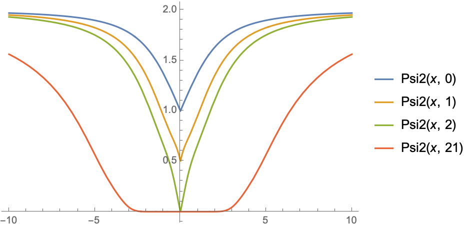
Figure 5: Functions Ψ1\Psi_{1} (left) and Ψ2\Psi_{2} (right) defined in (19) and (20) for b⁡(x)∝|x|kb(x)\propto|x|^{k} with k=0k=0 (blue), k=1k=1 (orange), k=2k=2 (green) and k=21k=21 (red)

The following properties of the functions defined in (19) and (20) (with τ∞\tau_{\infty} as given in (21)) will be useful as well (see Fig. 5 for illustration11 1 The supplementary material contains more information on these functions.): Ψ1\Psi_{1} and Ψ2\Psi_{2} are even and positive, and

  • •

    if k=0k=0 then Ψ1​(x)\Psi_{1}(x) is unimodal with maximum Ψ1​(0)=2/π\Psi_{1}(0)=\sqrt{2/\pi} at x=0x=0 and strictly decreasing towards 0 for x≥0x\geq 0; Ψ2​(x)\Psi_{2}(x) is unimodal with minimum Ψ2​(0)=1\Psi_{2}(0)=1 at x=0x=0 and strictly increasing towards 2 for x≥0x\geq 0.

  • •

    If k=1k=1 then Ψ1​(x)\Psi_{1}(x) is bimodal with minimum Ψ1​(0)=0\Psi_{1}(0)=0 at x=0x=0, maximum value less than 1 after which it is strictly decreasing towards 0 for x≥0x\geq 0; Ψ2​(x)\Psi_{2}(x) is unimodal with minimum Ψ2​(0)=1/2\Psi_{2}(0)=1/2 at x=0x=0 and strictly increasing towards 2 for x≥0x\geq 0.

  • •

    If k≥2k\geq 2 then Ψ1​(x)\Psi_{1}(x) is bimodal with minimum Ψ1​(0)=0\Psi_{1}(0)=0 at x=0x=0, maximum value less than 1 after which it is strictly decreasing towards 0 for x≥0x\geq 0; Ψ2​(x)\Psi_{2}(x) is unimodal with minimum Ψ2​(0)=0\Psi_{2}(0)=0 at x=0x=0 and strictly increasing towards 2 for x≥0x\geq 0.

Having presented the key elements of Stein’s method for radial distributions, we now give some properties of the corresponding approximating sequences. The following lemma, ensuring a unique symmetric and monotone solution to (4), is a routine extension of a result in [15, 16] to general kk. In the sequel we assume NN is even and define the median of an ordered set {x1,…,xN}\{x_{1},\ldots,x_{N}\} to be (xm+xm+1)/2(x_{m}+x_{m+1})/2, where m=N/2m=N/2.

Lemma 3.3.

Every zero-median solution {x1,…,xN}\{x_{1},\ldots,x_{N}\} of (4) for a given k≥0k\geq 0 satisfies:

    • (P1)

      Zero-mean: x1+…+xN=0x_{1}+\ldots+x_{N}=0.

    • (P2)

      Variance-bound: x12+…+xN2=(k+1)​(N−1)x_{1}^{2}+\ldots+x_{N}^{2}=(k+1)(N-1).

    • (P3)

      Symmetry: xn=−xN+1−nx_{n}=-x_{N+1-n} for n=1,…,Nn=1,\ldots,N.

Further, there exists a unique solution {x1,…,xN}\{x_{1},\ldots,x_{N}\} such that (P1) and

    • (P4)

      Strictly decreasing: x1>…>xNx_{1}>\ldots>x_{N}

hold. This solution has the zero-median property, and thus also satisfies (P2) and (P3).

Let 𝔽N{\mathbb{F}}_{N} be the empirical distribution of the unique solution {x1,…,xN}\left\{x_{1},\ldots,x_{N}\right\}. For the case k=0k=0, the following result gives the optimal rate of convergence in Wasserstein distance of 𝔽N{\mathbb{F}}_{N} to standard Gaussian. This result is not new, as the upper bound follows by adapting the coupling argument in [16], and the lower bound, which follows from a very delicate analysis of the xix_{i}’s, was recently proved in [3]. We provide a new proof for the upper bound in Example 3.7 below.

Proposition 3.2.

The empirical distribution 𝔽N\mathbb{F}_{N} on the unique symmetric and monotone solution to (1) (or (4) with k=0k=0) satisfies

dW⁡(𝔽N,𝔽∞)≍log⁡N/N,\displaystyle\mathop{d_{\mathrm{W}}}({\mathbb{F}}_{N},{\mathbb{F}}_{\infty})\asymp\sqrt{\log N}/N,

where 𝔽∞{\mathbb{F}}_{\infty} is the standard Gaussian distribution.

Upper bounds on the rate of convergence for values of k≥1k\geq 1 can also be obtained by adapting the arguments in [16] using the coupling approach (as developed in detail in the Supplementary material). The following result for the case k=1k=1 is based on this approach (and is detailed in Section 2.3 of the Supplementary material), but it is not expected to yield the optimal rate which, as argued in the sequel, we expect to be the same as the Gaussian case in the above proposition.

Proposition 3.3.

The empirical distribution 𝔽N\mathbb{F}_{N} on the unique symmetric and monotone solution to (5) (or (4) with k=1k=1) satisfies

dW⁡(𝔽N,𝔽∞)=O⁡(log⁡N/N),\displaystyle\mathop{d_{\mathrm{W}}}({\mathbb{F}}_{N},{\mathbb{F}}_{\infty})=O({\log N}/N),

where 𝔽∞{\mathbb{F}}_{\infty} is the two-sided Rayleigh distribution.

The main result of this section is the following theorem based on a discrete density approach to Stein’s method, cf. the approach of [8] in the case of points on an integer grid. This result is entirely new and may be of independent interest as the upper bound it provides does not rely on any specific structure of x1,…,xNx_{1},\ldots,x_{N} apart from symmetry and monotonicity, and therefore may be much more widely applicable. It leads to the new proof of the tight upper bound in Proposition 3.2 for the case k=0k=0, as shown in Example 3.7 below. For k≥1k\geq 1, it becomes more difficult analytically to determine the order of the bound, but it nevertheless provides a tight bound that can be evaluated numerically and that agrees with the asymptotic order of dW⁡(𝔽N,𝔽∞)\mathop{d_{\mathrm{W}}}({\mathbb{F}}_{N},{\mathbb{F}}_{\infty}) as N→∞N\to\infty, as discussed in Example 3.8 below.

Theorem 3.4.

Let NN be an even integer and x1,…,xNx_{1},\ldots,x_{N} be any symmetric and strictly monotone decreasing sequence. Set τN​(xi)=(xi−xi+1)​∑j=1ixj\tau_{N}(x_{i})=(x_{i}-x_{i+1})\sum_{j=1}^{i}x_{j} for 1≤i≤N−11\leq i\leq N-1, and τN​(xN)=0\tau_{N}(x_{N})=0. Let 𝔽N{\mathbb{F}}_{N} be the empirical distribution of these points and let 𝔽∞{\mathbb{F}}_{\infty} be the probability measure with density p∞p_{\infty} satisfying the assumptions of Proposition 3.1. Then

dW⁡(𝔽N,𝔽∞)\displaystyle\mathop{d_{\mathrm{W}}}({\mathbb{F}}_{N},{\mathbb{F}}_{\infty}) ≤1N​∑i=1N|τ∞​(xi)−τN​(xi)|​Ψ1​(xi)\displaystyle\leq\frac{1}{N}\sum_{i=1}^{N}\left|\tau_{\infty}(x_{i}){-\tau_{N}(x_{i})}\right|\Psi_{1}(x_{i}) (22)
+1N∑i=1N−1|xi−xi+1|τN(xi)max{Ψ2(xi),Ψ2(xi+1)},\displaystyle\quad+\frac{1}{N}\sum_{i=1}^{N-1}{|x_{i}-x_{i+1}|\tau_{N}(x_{i})}\max\{\Psi_{2}(x_{i}),\Psi_{2}(x_{i+1})\}, (23)

where Ψ1\Psi_{1} and Ψ2\Psi_{2} are given in (19) and (20), respectively.

Remark 3.5.

Equation (22) encourages us to consider the quantity τN​(xi)=(xi−xi+1)​∑j=1ixj\tau_{N}(x_{i})=(x_{i}-x_{i+1})\sum_{j=1}^{i}x_{j} as a Stein kernel for the uniform distribution on the set {x1,…,xN}\left\{x_{1},\ldots,x_{N}\right\}. This function is non-negative and, under the conditions that we are considering, it holds that τN​(x)≈τ∞​(x)\tau_{N}(x)\approx\tau_{\infty}(x) throughout the support of 𝔽N{\mathbb{F}}_{N} except close to the edges and the origin (see Figs. 6 and 7).

Refer to caption
Refer to caption
Refer to caption
Figure 6: Superimposition of τN​(xi),1≤i≤N\tau_{N}(x_{i}),1\leq i\leq N (orange bars) and τ∞​(xi),1≤i≤N\tau_{\infty}(x_{i}),1\leq i\leq N (blue bars) when τ∞​(x)=1+2/x2\tau_{\infty}(x)=1+2/x^{2} is the Stein kernel for the two-sided Maxwell distribution and (xi)1≤i≤N(x_{i})_{1\leq i\leq N} is as in Lemma 3.3 with k=2k=2 and N=20N=20 (left), N=110N=110 (middle) and N=300N=300 (right)
Refer to caption
Refer to caption
Refer to caption
Figure 7: Plot of |τN​(xi)−τ∞​(xi)|,1≤i≤N|\tau_{N}(x_{i})-\tau_{\infty}(x_{i})|,1\leq i\leq N when τ∞​(x)=1+2/x2\tau_{\infty}(x)=1+2/x^{2} is the Stein kernel for the two-sided Maxwell distribution and (xi)1≤i≤N(x_{i})_{1\leq i\leq N} is as in Lemma 3.3 with k=2k=2 and N=20N=20 (left), N=110N=110 (middle) and N=300N=300 (right)
Remark 3.6.

Since both Ψ1\Psi_{1} and Ψ2\Psi_{2} are uniformly bounded by 2, we immediately obtain the simpler upper bound

dW⁡(𝔽N,𝔽∞)\displaystyle\mathop{d_{\mathrm{W}}}({\mathbb{F}}_{N},{\mathbb{F}}_{\infty}) ≤1N​∑i=1N|τ∞​(xi)−τN​(xi)|+1N​∑i=1N−1|xi−xi+1|​τN​(xi).\displaystyle\leq\frac{1}{N}\sum_{i=1}^{N}\left|\tau_{\infty}(x_{i})-\tau_{N}(x_{i})\right|+\frac{1}{N}\sum_{i=1}^{N-1}|x_{i}-x_{i+1}|\tau_{N}(x_{i}).

This simplicity comes at the cost of a loss of precision in the rate. For instance, in the case that we consider here, the presence of the functions Ψ1\Psi_{1} and Ψ2\Psi_{2} in the bounds controls the problems around the origin.

Example 3.7 (Case k=0k=0).

The sequence {xn}\{x_{n}\} satisfies xn−xn+1=(∑i=1nxi)−1x_{n}-x_{n+1}=({\sum_{i=1}^{n}x_{i}})^{-1} so that τN​(xi)=1\tau_{N}(x_{i})=1 for all i=1,…,N−1i=1,\ldots,N-1. Since τ∞​(xi)=1\tau_{\infty}(x_{i})=1, (22) vanishes except for the term corresponding to i=Ni=N leading to Ψ1​(xN)/N≤1/N\Psi_{1}(x_{N})/N\leq 1/N. Also, (23) reads

1N​∑i=1N−1|xi+1−xi|​max⁡{Ψ2​(xi),Ψ2​(xi+1)}.\displaystyle\frac{1}{N}\sum_{i=1}^{N-1}|x_{i+1}-x_{i}|\max\{\Psi_{2}(x_{i}),\Psi_{2}(x_{i+1})\}.

Using Ψ2≤2\Psi_{2}\leq 2 along with the symmetry of the sequence, we then have

dW⁡(𝔽N,𝔽∞)≤1N+2N​∑i=1N−1|xi+1−xi|=1+4​x1N=O⁡(log⁡N/N),\displaystyle\mathop{d_{\mathrm{W}}}({\mathbb{F}}_{N},{\mathbb{F}}_{\infty})\leq\frac{1}{N}+\frac{2}{N}\sum_{i=1}^{N-1}|x_{i+1}-x_{i}|=\frac{1+4x_{1}}{N}=O(\sqrt{\log N}/N),

where the last step follows by a version of the argument in [16, Lemma 4.8] showing that x1=O⁡(log⁡N)x_{1}=O(\sqrt{\log N}). This proves the upper bound part of Proposition 3.2.

Example 3.8 (Cases k≥1k\geq 1).

Evaluating the bound in Theorem 3.4 based on numerical solutions to (4) and comparing the results with values of dW⁡(𝔽N,𝔽∞)\mathop{d_{\mathrm{W}}}(\mathbb{F}_{N},{\mathbb{F}}_{\infty}) calculated using numerical integration, over a range of values of NN, suggests that the bound is of the same order as dW⁡(𝔽N,𝔽∞)\mathop{d_{\mathrm{W}}}(\mathbb{F}_{N},{\mathbb{F}}_{\infty}), and moreover that

dW⁡(𝔽N,𝔽∞)≍log⁡N/N​ for ​k=1,2,\displaystyle\mathop{d_{\mathrm{W}}}({\mathbb{F}}_{N},{\mathbb{F}}_{\infty})\asymp\sqrt{\log N}/N\mbox{ for }k=1,2,
dW⁡(𝔽N,𝔽∞)≍(log⁡N)6/N2​ for ​k≥3.\displaystyle\mathop{d_{\mathrm{W}}}({\mathbb{F}}_{N},{\mathbb{F}}_{\infty})\asymp({\log N})^{6}/N^{2}\mbox{ for }k\geq 3.

To obtain these rates we used Mathematica to compute the bounds and R to compute the Wasserstein distance using its representation as the L1L_{1}-distance between the cdfs (the programs are provided in the Supplementary material).

Remark 3.9.

We emphasize that the bound in Theorem 3.4 holds irrespective of the sequence that is chosen; it may be of interest to optimize the approximation of p∞p_{\infty} by a sample x1<…<xNx_{1}<\ldots<x_{N} which minimizes the right hand side. One simple way to do this is to require that the sequence satisfies the recurrence

xi+1=xi−τ∞​(xi)∑j=1ixj,x_{i+1}=x_{i}-\frac{\tau_{\infty}(x_{i})}{\sum_{j=1}^{i}x_{j}},

thereby canceling out (22) and only leaving (23); note that in the Gaussian case τ∞=1\tau_{\infty}=1 so we are back with the recurrence (1).

Proof of Theorem 3.4.

The idea is to apply a version of Stein’s density method to FN∼𝔽NF_{N}\sim{\mathbb{F}}_{N}. Note that a discrete “derivative” at xix_{i}, i=1,…,N−1i=1,\ldots,N-1, is given by

DN​f​(xi)=f⁡(xi)−f⁡(xi+1).D_{N}f(x_{i})=f(x_{i})-f(x_{i+1}).

Writing σ⁡(xi)=∑j=1ixj\sigma(x_{i})=\sum_{j=1}^{i}x_{j}, straightforward summation (along with the identity xN=−∑j=1N−1xjx_{N}=-\sum_{j=1}^{N-1}x_{j}) shows

𝔼⁡[σ⁡(FN)​DN​g​(FN)−FN​g​(FN)]=0\mathbb{E}\left[\sigma(F_{N})D_{N}g(F_{N})-F_{N}g(F_{N})\right]=0

for all summable functions gg. Subtracting this from (16) applied to F=FNF=F_{N} gives

𝔼​h​(FN)−𝔼​h​(F∞)\displaystyle\mathbb{E}h(F_{N})-\mathbb{E}h(F_{\infty}) =𝔼⁡[τ∞​(FN)​g′​(FN)−FN​g​(FN)]\displaystyle=\mathbb{E}\left[\tau_{\infty}(F_{N})g^{\prime}(F_{N})-F_{N}g(F_{N})\right]
=𝔼⁡[τ∞​(FN)​g′​(FN)−σ⁡(FN)​DN​g​(FN)].\displaystyle=\mathbb{E}\left[\tau_{\infty}(F_{N})g^{\prime}(F_{N})-\sigma(F_{N})D_{N}g(F_{N})\right].

From (17) it then follows that

dW⁡(𝔽N,𝔽∞)≤suph∈ℋ|𝔼⁡[τ∞​(FN)​g′​(FN)−σ⁡(FN)​DN​g​(FN)]|\mathop{d_{\mathrm{W}}}(\mathbb{F}_{N},\mathbb{F}_{\infty})\leq\sup_{h\in\mathcal{H}}\left|\mathbb{E}\left[\tau_{\infty}(F_{N})g^{\prime}(F_{N})-\sigma(F_{N})D_{N}g(F_{N})\right]\right|

with g(=gh)g(=g_{h}) satisfying the bounds in Proposition 3.1. By Taylor’s theorem,

DN​f​(xi)=(xi−xi+1)​f′​(xi)−12​(xi−xi+1)2​f′′​(ci)​ for all ​1≤i≤N−1,\displaystyle D_{N}f(x_{i})={(x_{i}-x_{i+1})f^{\prime}(x_{i})-}{\small{1\over 2}}{(x_{i}-x_{i+1})^{2}}f^{\prime\prime}(c_{i}){\mbox{ for all }1\leq i\leq N-1,}

where cic_{i} is between xi+1x_{i+1} and xix_{i}. Hence

𝔼​h​(FN)−𝔼​h​(F∞)\displaystyle\mathbb{E}h(F_{N})-\mathbb{E}h(F_{\infty})
=1N​∑i=1N−1(τ∞​(xi)−σ⁡(xi)​(xi−xi+1))​g′​(xi)−12​N​∑i=1N−1σ⁡(xi)​(xi−xi+1)2​g′′​(ci)\displaystyle=\frac{1}{N}\sum_{i=1}^{{N-1}}\left(\tau_{\infty}(x_{i})-{\sigma(x_{i})}{(x_{i}-x_{i+1})}\right)g^{\prime}(x_{i}){{-}\frac{1}{2N}\sum_{i=1}^{{N-1}}{\sigma(x_{i})}({x_{i}-x_{i+1}})^{2}g^{\prime\prime}(c_{i})}
+τ∞​(xN)​g′​(xN)\displaystyle\qquad+\tau_{\infty}(x_{N})g^{\prime}(x_{N})
=1N​∑i=1N(τ∞​(xi)−τN​(xi))​g′​(xi)−12​N​∑i=1N−1(xi+1−xi)​τN​(xi)​g′′​(ci)\displaystyle=\frac{1}{N}\sum_{i=1}^{{N}}\left(\tau_{\infty}(x_{i})-\tau_{N}(x_{i})\right)g^{\prime}(x_{i})-\frac{1}{2N}\sum_{i=1}^{{N-1}}(x_{i+1}-x_{i})\tau_{N}(x_{i})g^{\prime\prime}(c_{i})

(recall that τN​(xN)=0\tau_{N}(x_{N})=0). Taking absolute values, using (19) and (20), along with the symmetry/unimodality of the function Ψ2\Psi_{2}, we get the result. ∎

4 Convergence of multidimensional ground states

In this section we apply the results of the previous section to the NN-point empirical distributions ℙN\mathbb{P}_{N} of the dd-dimensional ground states discussed in Sections 2.1 and 2.2.

These states have (signed) radial components given by the unique zero-median solution x1>…>xRx_{1}>\ldots>x_{R} to the recursion (4) with b⁡(x)=|x|kb(x)=|x|^{k}, where k=d−1≥1k=d-1\geq 1 and R=N1/2−1/(2​d)R=N^{1/2-1/(2d)} plays the role of NN in (4), corresponding to RR points in each of N1/2+1/(2​d)N^{1/2+1/(2d)} radial directions. By translating the results in Example 3.8 into the dd-dimensional setting, the optimal convergence rates of the radial part of ℙN\mathbb{P}_{N} to the radial part of the dd-dimensional normal distribution 𝒩d{\cal N}_{d} are seen to be given by

d=2,3d=2,3: dW⁡(ℙNradial,𝒩dradial)≍log⁡R/R\mathop{d_{\mathrm{W}}}(\mathbb{P}_{N}^{\rm radial},{\cal N}_{d}^{\rm radial})\asymp\sqrt{\log R}/R;

d≥4d\geq 4: dW⁡(ℙNradial,𝒩dradial)≍(log⁡R)6/R2\mathop{d_{\mathrm{W}}}(\mathbb{P}_{N}^{\rm radial},{\cal N}_{d}^{\rm radial})\asymp({\log R})^{6}/R^{2}.

The number of distinct polar angles in the directional part of the ground state (each with d−2d-2 components taking values in [0,π/2][0,\pi/2] when d≥3d\geq 3, and a single component in [0,π)[0,\pi) when d=2d=2) is of order N1/dN^{1/d}. For d≥3d\geq 3, a larger number (namely N1/2−1/(2​d)N^{1/2-1/(2d)}) of azimuthal angles corresponding to each polar angle are available, so the polar part has the slower convergence rate. In general, the Wasserstein distance between the directional part of ℙN\mathbb{P}_{N} and that of 𝒩d{\cal N}_{d} is thus of order N−1/dN^{-1/d} (this follows easily using the representation of Wasserstein distance as the L1L_{1}-distance between two cdfs). For d≥4d\geq 4, in view of the upper bound in Lemma 2.1, namely a sum involving separate contributions from the the radial part and the directional parts, we conclude that the overall rate that ℙN\mathbb{P}_{N} tends to 𝒩d{\cal N}_{d} is of order N−1/dN^{-1/d}. For d=3d=3, the radial component involving N1/3N^{1/3} points dominates, however, so the overall rate is of order log⁡N/N1/3\sqrt{\log N}/N^{1/3}. Similarly, the radial component involving N1/4N^{1/4} points dominates in the case d=2d=2, so the overall rate is of order log⁡N/N1/4\sqrt{\log N}/N^{1/4}.

In summary, we obtain

d=2d=2: dW⁡(ℙN,𝒩d)≍log⁡N/N1/4\mathop{d_{\mathrm{W}}}(\mathbb{P}_{N},{\cal N}_{d})\asymp\sqrt{\log N}/N^{1/4};

d=3d=3: dW⁡(ℙN,𝒩d)≍log⁡N/N1/3\mathop{d_{\mathrm{W}}}(\mathbb{P}_{N},{\cal N}_{d})\asymp\sqrt{\log N}/N^{1/3};

d≥4d\geq 4: dW(ℙN,𝒩d)≍N−1/d\mathop{d_{\mathrm{W}}}(\mathbb{P}_{N},{\cal N}_{d})\asymp N^{-1/d}.

Interestingly, the fastest rate of convergence to the ground state occurs in three dimensions.

For the excited states discussed in Section 2.3, the rates of convergence are of order N−1/dN^{-1/d}; in this case the directional components dominate because the radial component has the faster rate (as seen by applying Example 3.8 with k=d+1k=d+1 for d=2,3d=2,3).

References

  • [1] J. S. Brauchart and P. J. Grabner. Distributing many points on spheres: Minimal energy and designs. Journal of Complexity, 31(3):293 – 326, 2015.
  • [2] L. H. Y. Chen, L. Goldstein, and Q.-M. Shao. Normal approximation by Stein’s method. Probability and its Applications (New York). Springer, Heidelberg, 2011.
  • [3] L. H. Chen and L. V. Thành. Optimal bounds in normal approximation for many interacting worlds. arXiv:2006.11027, 2020.
  • [4] C. Döbler. Stein’s method of exchangeable pairs for the Beta distribution and generalizations. Electronic Journal of Probability, 20(109):1–34, 2015.
  • [5] M. Ernst, G. Reinert, and Y. Swan. First-order covariance inequalities via Stein’s method. Bernoulli, 26(3):2051–2081, 2020.
  • [6] M. Ernst and Y. Swan. Distances between distributions via Stein’s method. Journal of Theoretical Probability, 2020.
  • [7] M. Ghadimi, M. J. W. Hall, and H. M. Wiseman. Nonlocality in Bell’s theorem, in Bohm’s theory, and in many interacting worlds theorising. Entropy, 20(8), 2018.
  • [8] L. Goldstein and G. Reinert. Stein’s method for the Beta distribution and the Pólya-Eggenberger urn. Journal of Applied Probability, 50(4):1187–1205, 2013.
  • [9] M. J. W. Hall, D.-A. Deckert, and H. M. Wiseman. Quantum phenomena modeled by interactions between many classical worlds. Physical Review X, 4:041013, Oct 2014.
  • [10] H. Herrmann, M. J. W. Hall, H. M. Wiseman, and D. A. Deckert. Ground states in the many interacting worlds approach. arXiv:1712.01918, 2018.
  • [11] G. Jameson. The incomplete gamma functions. The Mathematical Gazette, 100(548):298–306, 2016.
  • [12] C. Ley, G. Reinert, and Y. Swan. Distances between nested densities and a measure of the impact of the prior in Bayesian statistics. The Annals of Applied Probability, 27(1):216–241, 2017.
  • [13] S. Li. Concise formulas for the area and volume of a hyperspherical cap. Asian Journal of Mathematics and Statistics, 4:66–70, 2011.
  • [14] E. Mariucci and M. Reiß. Wasserstein and total variation distance between marginals of Lévy processes. Electronic Journal of Statistics, 12(2):2482–2514, 2018.
  • [15] I. W. McKeague and B. Levin. Convergence of empirical distributions in an interpretation of quantum mechanics. The Annals of Applied Probability, 26(4):2540–2555, 2016.
  • [16] I. W. McKeague, E. A. Peköz, and Y. Swan. Stein’s method and approximating the quantum harmonic oscillator. Bernoulli, 25(1):89–111, 02 2019.

Appendix A Supplementary material

All code for performing computations is available at the url

https://tinyurl.com/mcks2021code

The code is also available at the end of the supplementary material.

A.1 Preliminary remarks on Stein operators

Consider a probability distribution ℙ\mathbb{P} with cdf PP, pdf pp w.r.t. the Lebesgue measure on ℝ\mathbb{R}. Suppose that pp itself is absolutely continuous, with a.e. derivative p′​(x)p^{\prime}(x). We denote L1​(p)L^{1}(p) the collection of functions such that ∫−∞∞|h⁡(x)|​p​(x)​𝑑x<∞\int_{-\infty}^{\infty}|h(x)|p(x)\mathrm{d}x<\infty and write P⁡(h)=𝔼p​h=∫−∞∞h⁡(x)​p​(x)​𝑑x.P(h)=\mathbb{E}_{p}h=\int_{-\infty}^{\infty}h(x)p(x)\mathrm{d}x. We also denote ℱ(0)​(p)\mathcal{F}^{(0)}(p) the collection of all mean 0 functions under pp. Following [5], to pp we associate the Stein operators

𝒯p​f​(x)=(f⁡(x)​p​(x))′p⁡(x)\displaystyle\mathcal{T}_{p}f(x)=\frac{(f(x)p(x))^{\prime}}{p(x)} (24)
ℒp​h​(x)=1p⁡(x)​∫−∞x(h⁡(u)−P⁡(h))​p​(u)​𝑑u\displaystyle\mathcal{L}_{p}h(x)=\frac{1}{p(x)}\int_{-\infty}^{x}(h(u)-P(h))p(u)\mathrm{d}u (25)

with the convention that 𝒯p​f​(x)=ℒp​h​(x)=0\mathcal{T}_{p}f(x)=\mathcal{L}_{p}h(x)=0 for all xx such that p⁡(x)=0p(x)=0. In the sequel we denote 𝒮⁡(p)={x|p⁡(x)>0}\mathcal{S}(p)=\left\{x\,|\,p(x)>0\right\}, a=inf𝒮⁡(p)a=\inf\mathcal{S}(p) and b=sup𝒮⁡(p)b=\sup\mathcal{S}(p); we assume that 𝒮⁡(p)\mathcal{S}(p) is the union of a finite number of intervals.

Of course (24) is only defined for functions ff such that f​pfp is absolutely continuous. We denote ℱ⁡(p)\mathcal{F}(p) the collection of functions ff such that not only is f​pfp absolutely continuous, but also (f⁡(x)​p​(x))′∈L1​(p)(f(x)p(x))^{\prime}\in L^{1}(p) and limx→af⁡(x)​p​(x)=limx→bf⁡(x)​p​(x)=0\lim_{x\to a}f(x)p(x)=\lim_{x\to b}f(x)p(x)=0. This class of functions is important because 𝒯p​f∈ℱ(0)​(p)\mathcal{T}_{p}f\in\mathcal{F}^{(0)}(p) for all f∈ℱ⁡(p)f\in\mathcal{F}(p); this is crucial for Stein’s method as it gives rise to many “Stein identities” which can be used for a variety of purposes. Similarly, (25) is only defined for functions h∈L1​(p)h\in L^{1}(p), in which case ℒp​h∈ℱ⁡(p)\mathcal{L}_{p}h\in\mathcal{F}(p) for all h∈L1​(p)h\in L^{1}(p).

As described in [12], it is interesting to “standardize” the operator (24) by fixing some c∈ℱ⁡(p)c\in\mathcal{F}(p) and considering the family of “standardized Stein operators” 𝒜c​f​(x)=𝒯p​(c​f)​(x)=c⁡(x)​f′​(x)+(c′​(x)+p′​(x)/p⁡(x)​c​(x))​f​(x)\mathcal{A}_{c}f(x)=\mathcal{T}_{p}(cf)(x)=c(x)f^{\prime}(x)+\Big(c^{\prime}(x)+{p^{\prime}(x)}/{p(x)}c(x)\Big)f(x) acting on some class ℱ⁡(𝒜c)\mathcal{F}(\mathcal{A}_{c}) made of all functions for which c​f∈ℱ⁡(p)cf\in\mathcal{F}(p). Note that, by definition, we have 𝔼⁡[𝒜c​f​(X)]=0\mathbb{E}[\mathcal{A}_{c}f(X)]=0 for all f∈ℱ⁡(𝒜c)f\in\mathcal{F}(\mathcal{A}_{c}). It is important that cc be well-chosen to ensure that 𝒜c\mathcal{A}_{c} has a manageable expression; as is now well known, there are many instances of densities pp (even intractable densities) for which this turns out to be possible, leading to many powerful handles on pp which can then serve for a variety of purposes including but not limited to distributional approximation.

Given an operator 𝒜c\mathcal{A}_{c}, classical instantiations of Stein’s method begin with a “Stein equation”, i.e. a differential equation of the form

𝒜c​f​(x)=h⁡(x)−P⁡(h)\mathcal{A}_{c}f(x)=h(x)-P(h) (26)

for hh some function belonging to a class ℋ\mathcal{H} of test functions. Typically, Stein’s method practitionners work with one of the following classes: (i) h∈ℋ:=Kol(ℝ)={𝕀(−∞,z],z∈ℝ}h\in\mathcal{H}:=\mathrm{Kol}(\mathbb{R})=\left\{\mathbb{I}(-\infty,z],z\in\mathbb{R}\right\} the indicators of a lower half line; (ii) h∈ℋ:=TV⁡(ℝ)h\in\mathcal{H}:=\mathrm{TV}(\mathbb{R}) the collection of functions such that ‖h‖≤1\|h\|\leq 1; (iii) h∈ℋ:=Wass⁡(ℝ)h\in\mathcal{H}:=\mathrm{Wass}(\mathbb{R}) the collection of Lipschitz functions such that ‖h′‖≤1\|h^{\prime}\|\leq 1. In the sequel, we restrict our attention to ℋ=Wass⁡(ℝ)\mathcal{H}=\mathrm{Wass}(\mathbb{R}), and we assume that for each h∈ℋh\in\mathcal{H} there exists a unique function f∈ℱ⁡(𝒜c)f\in\mathcal{F}(\mathcal{A}_{c}) for which (26) holds for all x∈𝒮⁡(p)x\in\mathcal{S}(p). Under “reasonable assumptions on pp” (to be verified on a case-by-case basis) we can write 𝒯p​ℒp​h=h−𝔼p​h\mathcal{T}_{p}\mathcal{L}_{p}h=h-\mathbb{E}_{p}h for all h∈L1​(p)h\in L^{1}(p) and in particular 𝒯p​ℒp=Id\mathcal{T}_{p}\mathcal{L}_{p}=\mathrm{Id} over ℱ(0)​(p)\mathcal{F}^{(0)}(p) (Id\mathrm{Id} is the identity function). Similarly ℒp​𝒯p=Id\mathcal{L}_{p}\mathcal{T}_{p}=\mathrm{Id} over ℱ⁡(p)\mathcal{F}(p). In other words, under “reasonable assumptions on pp”, the solution to (26) is fh​(x)=ℒp​h​(x)/c⁡(x)f_{h}(x)={\mathcal{L}_{p}h(x)}/{c(x)} at all x∈𝒮⁡(p)x\in\mathcal{S}(p) for which c⁡(x)≠0c(x)\neq 0. Then, since the Wasserstein distance between two probability measures ℙ\mathbb{P} and ℚ\mathbb{Q} can be written as dW⁡(ℙ,ℚ)=suph∈Wass⁡(ℝ)|𝔼​h​(X)−𝔼​h​(Y)|\mathop{d_{\mathrm{W}}}(\mathbb{P},\mathbb{Q})=\sup_{h\in\mathrm{Wass}(\mathbb{R})}|\mathbb{E}h(X)-\mathbb{E}h(Y)| where X∼ℙX\sim\mathbb{P} and Y∼ℚY\sim\mathbb{Q}, it holds that

dW⁡(ℙ,ℚ)=suph∈Wass⁡(1)|𝔼⁡[𝒜c​fh​(Y)]|;\mathop{d_{\mathrm{W}}}(\mathbb{P},\mathbb{Q})=\sup_{h\in\mathrm{Wass}(1)}\left|\mathbb{E}\left[\mathcal{A}_{c}f_{h}(Y)\right]\right|; (27)

Stein’s method in Wasserstein distance consists in exploiting this last identity for the purpose of estimating the Wasserstein distance between the laws ℙ\mathbb{P} and ℚ\mathbb{Q}.

In order to be able to use (27) successfully, it is crucial to control solutions fhf_{h} and their derivatives. In [6] the following representations for (25) are provided (recall that hh is Lipschitz with a.e. derivative h′h^{\prime}):

−ℒp​h​(x)\displaystyle-\mathcal{L}_{p}h(x) =−𝔼⁡[(h⁡(X)−P⁡(h))​𝕀[X≤x]p⁡(x)]\displaystyle=-\mathbb{E}\left[({h}(X)-P(h))\frac{\mathbb{I}[X\leq x]}{p(x)}\right]
=−𝔼⁡[(h⁡(X)−P⁡(h))​𝕀[X≤x]−P(x)p⁡(x)]\displaystyle=-\mathbb{E}\left[({h}(X)-P(h))\frac{\mathbb{I}[X\leq x]-P(x)}{p(x)}\right]
=𝔼⁡[(h⁡(X2)−h⁡(X1))​𝕀[X1≤x≤X2]p⁡(x)]\displaystyle=\mathbb{E}\left[(h(X_{2})-h(X_{1}))\frac{\mathbb{I}[X_{1}\leq x\leq X_{2}]}{p(x)}\right] (28)
=𝔼⁡[h′​(X)​P⁡(x∧X)​(1−P⁡(x∨X))p⁡(x)​p​(X)]\displaystyle=\mathbb{E}\left[h^{\prime}(X)\frac{P(x\wedge X)(1-P(x\lor X))}{p(x)p(X)}\right] (29)

where, in (28), the random variables X1,X2X_{1},X_{2} are independent copies of XX. A simpler way to write (29) is

−ℒp​h​(x)=∫−∞∞h′​(y)​P∞​(y∧x)​P¯∞​(y∨x)p∞​(x)​𝑑y\displaystyle-\mathcal{L}_{p}h(x)=\int_{-\infty}^{\infty}h^{\prime}(y)\frac{P_{\infty}(y\wedge x)\bar{P}_{\infty}(y\lor x)}{p_{\infty}(x)}\mathrm{d}y

It is also shown that

h¯​(x):=h⁡(x)−P⁡(h)=𝔼⁡[h′​(X)​P(X)−𝕀[x≤X]p⁡(X)]\displaystyle\bar{h}(x):=h(x)-P(h)=\mathbb{E}\left[h^{\prime}(X)\frac{P(X)-\mathbb{I}[x\leq X]}{p(X)}\right]

for all x∈𝒮⁡(p)x\in\mathcal{S}(p). All these representations will be used in the next section to control the solutions to the Stein equations; this in turn will lead to the distributional approximation results.

A.2 Stein’s method for radial distributions

A.2.1 Notations and background

Before specializing to radial densities, it is enlightening to first widen the scope somewhat and consider targets F∞F_{\infty} with density of the form p∞​(x)=b⁡(x)​γ​(x)p_{\infty}(x)=b(x)\gamma(x), for γ\gamma some “basis density” and bb some positive γ\gamma-integrable “tilting” function. This theory may also be of independent interest.

First note that, in order for p∞p_{\infty} to be a density, it is necessary that b≥0∈L1​(γ)b\geq 0\in L^{1}(\gamma) and 𝔼⁡[b⁡(Z)]=1\mathbb{E}[b(Z)]=1, where here and throughout we denote Z∼γZ\sim\gamma. We further impose the following assumptions on p∞p_{\infty}. First, we require that γ\gamma is a differentiable probability density function with support the full real line, such that moreover γ′∈L1​(d​x)\gamma^{\prime}\in L^{1}(\mathrm{d}x) has exactly one sign change (which, for simplicity, we fix at 0) and ∫γ′​(x)​𝑑x=0\int\gamma^{\prime}(x)\mathrm{d}x=0. Second, we let B⁡(x)B(x) be an absolutely continuous nondecreasing function with continuous derivative bb, we denote 𝒮B={x∈ℝ\mathcal{S}_{B}=\left\{x\in\mathbb{R}\right., such that b(x)>0}\left.b(x)>0\right\} and suppose that 𝒮B\mathcal{S}_{B} is the union of a finite number of intervals. Following [12], we also introduce ℱ⁡(γ)\mathcal{F}(\gamma) the Stein class of γ\gamma; this is the class of functions f:ℝ→ℝf:\mathbb{R}\to\mathbb{R} such that (f​γ)′∈L1​(d​x)(f\gamma)^{\prime}\in L^{1}(\mathrm{d}x) and ∫ℝ(f⁡(x)​γ​(x))′​𝑑x=0\int_{\mathbb{R}}(f(x)\gamma(x))^{\prime}\mathrm{d}x=0. We assume that B∈ℱ⁡(γ)B\in\mathcal{F}(\gamma); since b∈L1​(γ)b\in L^{1}(\gamma), this assures us that ∫bγ=−∫Bγ′\int b\gamma=-\int B\gamma^{\prime} so that integration by parts holds without a remainder term. Finally, letting F∞∼p∞F_{\infty}\sim p_{\infty}, we impose that 𝔼​F∞(=𝔼⁡[Z​b​(Z)])=0\mathbb{E}F_{\infty}(=\mathbb{E}[Zb(Z)])=0.

With these assumptions we are now ready to provide a Stein’s method theory for p∞=b​γp_{\infty}=b\gamma; the backbone of our approach comes from [16].

Definition A.1 (Generalized (b,γ)(b,\gamma)-bias transformation).

Suppose that FF is such that P⁡(F∈𝒮B)=1P(F\in\mathcal{S}_{{B}})=1 and define

σB2​(F)=𝔼⁡[−γ′​(F)γ⁡(F)​B⁡(F)b⁡(F)].\displaystyle\sigma^{2}_{B}(F)=\mathbb{E}\left[-\frac{\gamma^{\prime}(F)}{\gamma(F)}\frac{B(F)}{b(F)}\right].

The random variable F⋆F^{\star} satisfying

σB2​(F)​𝔼​[f′​(F⋆)b⁡(F⋆)]=𝔼⁡[−γ′​(F)γ⁡(F)​f⁡(F)b⁡(F)]\displaystyle\sigma^{2}_{B}(F)\mathbb{E}\left[\frac{f^{\prime}(F^{\star})}{b(F^{\star})}\right]=\mathbb{E}\left[-\frac{\gamma^{\prime}(F)}{\gamma(F)}\frac{f(F)}{b(F)}\right]

for all ff such that both integrals exist is said to have the generalized (b,γ)(b,\gamma)-bias distribution. The random variable F⋆F^{\star} is the generalized (b,γ)(b,\gamma)-bias transform of FF.

By construction, we always have

σB2​(F∞)\displaystyle\sigma^{2}_{B}(F_{\infty}) =𝔼[−γ′​(F∞)γ⁡(F∞)B⁡(F∞)b⁡(F∞)]=−∫𝒮Bγ′(x)B(x)dx=∫𝒮Bb(x)γ(x)dx=𝔼b(Z)=1.\displaystyle=\mathbb{E}\left[-\frac{\gamma^{\prime}(F_{\infty})}{\gamma(F_{\infty})}\frac{B(F_{\infty})}{b(F_{\infty})}\right]=-\int_{\mathcal{S}_{B}}\gamma^{\prime}(x)B(x)\mathrm{d}x=\int_{\mathcal{S}_{B}}b(x)\gamma(x)\mathrm{d}x=\mathbb{E}b(Z)=1.

Moreover, for any sufficiently regular function ff:

𝔼⁡[−γ′​(F∞)γ⁡(F∞)​f⁡(F∞)b⁡(F∞)]=𝔼⁡[f′​(F∞)b⁡(F∞)].\displaystyle\mathbb{E}\left[-\frac{\gamma^{\prime}(F_{\infty})}{\gamma(F_{\infty})}\frac{f(F_{\infty})}{b(F_{\infty})}\right]=\mathbb{E}\left[\frac{f^{\prime}(F_{\infty})}{b(F_{\infty})}\right].

Therefore F∞=F⋆F_{\infty}=F^{\star}, i.e. p∞p_{\infty} is a fixed point of the generalized (b,γ)(b,\gamma)-bias transform. More generally, the following holds true.

Lemma A.2.

If σB2​(F)<∞\sigma^{2}_{B}(F)<\infty then its generalized (b,γ)(b,\gamma)-bias transform F⋆F^{\star} exits and is absolutely continuous with density

p⋆(x)=−b⁡(x)σB2​(F)𝔼[1b⁡(F)γ′​(F)γ⁡(F)𝕀[F≥x]].\displaystyle p^{\star}(x)=-\frac{b(x)}{\sigma^{2}_{B}(F)}\mathbb{E}\left[\frac{1}{b(F)}\frac{\gamma^{\prime}(F)}{\gamma(F)}\mathbb{I}[F\geq x]\right].

Moreover F∞F_{\infty} is the unique fixed point of this tranformation, in the sense that if F=𝒟F⋆{F}\stackrel{{\scriptstyle\mathcal{D}}}{{=}}F^{\star} then F=𝒟F∞F\stackrel{{\scriptstyle\mathcal{D}}}{{=}}F_{\infty} (equality in distribution).

Proof.

The proof of unicity is easy; the other points follow from arguments nearly identical to those in [2, Proposition 2.1]. ∎

Now consider the function

f⁡(x)=1γ⁡(x)​∫−∞x(h⁡(u)−𝔼​h​(F∞))​b​(u)​γ​(u)​𝑑u=:1γ⁡(x)​∫−∞xh¯​(u)​b​(u)​γ​(u)​𝑑u\displaystyle f(x)=\frac{1}{\gamma(x)}\int_{-\infty}^{x}\big(h(u)-\mathbb{E}h(F_{\infty})\big)b(u)\gamma(u)\mathrm{d}u=:\frac{1}{\gamma(x)}\int_{-\infty}^{x}\bar{h}(u)b(u)\gamma(u)\mathrm{d}u

which is solution to the differential equation

(h¯​(x):=)​h​(x)−𝔼​h​(F∞)=f′​(x)+γ′​(x)/γ⁡(x)​f​(x)b⁡(x)\displaystyle(\bar{h}(x):=)h(x)-\mathbb{E}h(F_{\infty})=\frac{f^{\prime}(x)+\gamma^{\prime}(x)/\gamma(x)f(x)}{b(x)}

for all x∈𝒮Bx\in\mathcal{S}_{B}. Let FF be a random variable such that P⁡(F∈𝒮B)=1P(F\in\mathcal{S}_{B})=1 and σB2​(F)=1\sigma^{2}_{B}(F)=1. We have

𝔼​h​(F)−𝔼​h​(F∞)=𝔼⁡[f′​(F)b⁡(F)+γ′​(F)γ⁡(F)​f⁡(F)b⁡(F)]=𝔼⁡[f′​(F)b⁡(F)−f′​(F⋆)b⁡(F⋆)]\displaystyle\mathbb{E}h(F)-\mathbb{E}h(F_{\infty})=\mathbb{E}\left[\frac{f^{\prime}(F)}{b(F)}+\frac{\gamma^{\prime}(F)}{\gamma(F)}\frac{f(F)}{b(F)}\right]=\mathbb{E}\left[\frac{f^{\prime}(F)}{b(F)}-\frac{f^{\prime}(F^{\star})}{b(F^{\star})}\right] (30)

and it remains to express the right hand side of (30) in terms of manageable quantities, such as moments of F,F⋆F,F^{\star} and F−F⋆F-F^{\star}. We cannot work directly with the function x↦f′​(x)/b⁡(x)x\mapsto f^{\prime}(x)/b(x) because the latter is unbounded at x=0x=0. To bypass this difficulty, we introduce the notation

ℒ∞​h​(x)=1p∞​(x)​∫−∞xh¯​(u)​p∞​(u)​𝑑u\mathcal{L}_{\infty}h(x)=\frac{1}{p_{\infty}(x)}\int_{-\infty}^{x}\bar{h}(u)p_{\infty}(u)\mathrm{d}u

(we stress that OPENℒ∞≠ℒγ)\mathcal{L}_{\infty}\neq\mathcal{L}_{\gamma}) and follow [16] by introducing the function g=gη,hg=g_{\eta,h} given by

g⁡(x)=ℒ∞​h​(x)ℒ∞​η​(x)=∫−∞x(h⁡(u)−𝔼​h​(F∞))​b​(u)​γ​(u)​𝑑u∫−∞x(η⁡(u)−𝔼​η​(F∞))​b​(u)​γ​(u)​𝑑u\displaystyle g(x)=\frac{\mathcal{L}_{\infty}h(x)}{\mathcal{L}_{\infty}\eta(x)}=\frac{\int_{-\infty}^{x}(h(u)-\mathbb{E}h(F_{\infty}))b(u)\gamma(u)\mathrm{d}u}{\int_{-\infty}^{x}(\eta(u)-\mathbb{E}\eta(F_{\infty}))b(u)\gamma(u)\mathrm{d}u} (31)

at all x∈𝒮Bx\in\mathcal{S}_{B} where hh is fixed by the left hand side of (30) but η\eta is kept unspecified, to be tuned to our needs at a later stage. Obviously, the above relations are only defined at xx such that p∞​(x)≠0p_{\infty}(x)\neq 0; we suppose this to be the case here and in the sequel. The function gg from (31) is then solution to the Stein equation

(ℒ∞​η​(x))​g′​(x)+η¯​(x)​g​(x)=h⁡(x)−𝔼​h​(F∞)\displaystyle\left(\mathcal{L}_{\infty}\eta(x)\right)g^{\prime}(x)+\bar{\eta}(x)g(x)=h(x)-\mathbb{E}h(F_{\infty})

at all xx inside the support of p∞p_{\infty}. It will be useful to note that the functions g,hg,h and η\eta satisfy the relations

(ℒ∞​η)​g\displaystyle(\mathcal{L}_{\infty}\eta)g =ℒ∞​h\displaystyle=\mathcal{L}_{\infty}h
(ℒ∞​η)​g′\displaystyle(\mathcal{L}_{\infty}\eta)g^{\prime} =h¯−η¯​g=h¯−η¯​ℒ∞​hℒ∞​η\displaystyle=\overline{h}-\overline{\eta}g=\overline{h}-\overline{\eta}\frac{\mathcal{L}_{\infty}h}{\mathcal{L}_{\infty}\eta}
(ℒ∞​η)​g′′\displaystyle(\mathcal{L}_{\infty}\eta)g^{\prime\prime} =h′−(η¯+(ℒ∞​η)′)​g′−η′​g\displaystyle=h^{\prime}-(\overline{\eta}+(\mathcal{L}_{\infty}\eta)^{\prime})g^{\prime}-\eta^{\prime}g (32)
=(η¯​η¯+(ℒ∞​η)′ℒ∞​η−η′)​g−(h¯​η¯+(ℒ∞​η)′ℒ∞​η−h′).\displaystyle=\left(\overline{\eta}\frac{\overline{\eta}+\left(\mathcal{L}_{\infty}\eta\right)^{\prime}}{\mathcal{L}_{\infty}\eta}-\eta^{\prime}\right)g-\left(\overline{h}\frac{\overline{\eta}+\left(\mathcal{L}_{\infty}\eta\right)^{\prime}}{\mathcal{L}_{\infty}\eta}-h^{\prime}\right).

Straightforward manipulations of the definitions also lead to

ℒ∞​h​(x)=ℒγ​(h​b)​(x)b⁡(x)−𝔼⁡[h⁡(Z)​b​(Z)]​ℒγ​b​(x)b⁡(x).\displaystyle\mathcal{L}_{\infty}h(x)=\frac{\mathcal{L}_{\gamma}(hb)(x)}{b(x)}-\mathbb{E}[h(Z)b(Z)]\frac{\mathcal{L}_{\gamma}b(x)}{b(x)}.

Finally we note that gg and ff are related through f⁡(x)=ℒ∞​η​(x)​g​(x)​b​(x)f(x)=\mathcal{L}_{\infty}\eta(x)g(x)b(x) so that

f′​(x)b⁡(x)=ℒ∞​η​(x)​g′​(x)+(η¯​(x)−γ′​(x)γ⁡(x)​ℒ∞​η​(x))​g​(x)=:ℒ∞​η​(x)​g′​(x)+Ψ∞​η​(x)​g​(x).\displaystyle\frac{f^{\prime}(x)}{b(x)}=\mathcal{L}_{\infty}\eta(x)g^{\prime}(x)+\left(\overline{\eta}(x)-\frac{\gamma^{\prime}(x)}{\gamma(x)}\mathcal{L}_{\infty}\eta(x)\right)g(x)=:\mathcal{L}_{\infty}\eta(x)g^{\prime}(x)+\Psi_{\infty}\eta(x)g(x).

Identity (30) becomes

𝔼​h​(F)−𝔼​h​(F∞)\displaystyle\mathbb{E}h(F)-\mathbb{E}h(F_{\infty}) =𝔼⁡[ℒ∞​η​(F)​g′​(F)−ℒ∞​η​(F⋆)​g′​(F⋆)]\displaystyle=\mathbb{E}\Big[\mathcal{L}_{\infty}\eta(F)g^{\prime}(F)-\mathcal{L}_{\infty}\eta(F^{\star})g^{\prime}(F^{\star})\Big]
+𝔼⁡[Ψ∞​η​(F)​g​(F)−Ψ∞​η​(F⋆)​g​(F⋆)]\displaystyle\quad+\mathbb{E}\Big[\Psi_{\infty}\eta(F)g(F)-\Psi_{\infty}\eta(F^{\star})g(F^{\star})\Big] (33)

which is close to what is required. This is however not exactly what we need because, although we shall see that for reasonable choices of η\eta, the function gg from (31) and its derivative g′g^{\prime} are bounded, the second derivative g′′g^{\prime\prime} is often not. In order to cater for this, we introduce some further degrees of liberty in the expressions and rewrite (33) as

𝔼​h​(F)−𝔼​h​(F∞)=𝔼⁡[(r1​(F)​ℒ∞​η​(F)−r1​(F⋆)​ℒ∞​η​(F⋆))​g′​(F⋆)r1​(F⋆)]\displaystyle\mathbb{E}h(F)-\mathbb{E}h(F_{\infty})=\mathbb{E}\Big[\Big(r_{1}(F)\mathcal{L}_{\infty}\eta(F)-r_{1}(F^{\star})\mathcal{L}_{\infty}\eta(F^{\star})\Big)\frac{g^{\prime}(F^{\star})}{r_{1}(F^{\star})}\Big]
+𝔼⁡[r1​(F)​ℒ∞​η​(F)​(g′​(F)r1​(F)−g′​(F⋆)r1​(F⋆))]\displaystyle\quad+\mathbb{E}\Big[r_{1}(F)\mathcal{L}_{\infty}\eta(F)\Big(\frac{g^{\prime}(F)}{r_{1}(F)}-\frac{g^{\prime}(F^{\star})}{r_{1}(F^{\star})}\Big)\Big]
+𝔼⁡[(r2​(F)​Ψ∞​η​(F)−r2​(F⋆)​Ψ∞​η​(F⋆))​g⁡(F⋆)r2​(F⋆)]\displaystyle\quad+\mathbb{E}\Big[\Big(r_{2}(F)\Psi_{\infty}\eta(F)-r_{2}(F^{\star})\Psi_{\infty}\eta(F^{\star})\Big)\frac{g(F^{\star})}{r_{2}(F^{\star})}\Big]
+𝔼⁡[r2​(F)​Ψ∞​η​(F)​(g⁡(F)r2​(F)−g⁡(F⋆)r2​(F⋆))],\displaystyle\quad+\mathbb{E}\Big[r_{2}(F)\Psi_{\infty}\eta(F)\Big(\frac{g(F)}{r_{2}(F)}-\frac{g(F^{\star})}{r_{2}(F^{\star})}\Big)\Big],

with r1,r2r_{1},r_{2} two functions left to be determined with the aim of tempering the malevolent intentions of g′g^{\prime} and g′′g^{\prime\prime}. These considerations lead to the main result of the Section.

Proposition A.1.

Let the previous notations and assumptions prevail. Then

|𝔼​h​(F)−𝔼​h​(F∞)|\displaystyle\left|\mathbb{E}h(F)-\mathbb{E}h(F_{\infty})\right|
≤κ1​𝔼​[|r1​(F)​ℒ∞​η​(F)−r1​(F⋆)​ℒ∞​η​(F⋆)|]+κ2​𝔼​[|r1​(F)​ℒ∞​η​(F)|​|F−F⋆|]\displaystyle\leq\kappa_{1}\mathbb{E}\Big[\Big|r_{1}(F)\mathcal{L}_{\infty}\eta(F)-r_{1}(F^{\star})\mathcal{L}_{\infty}\eta(F^{\star})\Big|\Big]+\kappa_{2}\mathbb{E}\Big[|r_{1}(F)\mathcal{L}_{\infty}\eta(F)||F-F^{\star}|\Big]
+κ3​𝔼​[|r2​(F)​Ψ∞​η​(F)−r2​(F⋆)​Ψ∞​η​(F⋆)|]+κ4​𝔼​[|r2​(F)​Ψ∞​η​(F)|​|F−F⋆|]\displaystyle\quad+\kappa_{3}\mathbb{E}\Big[\Big|r_{2}(F)\Psi_{\infty}\eta(F)-r_{2}(F^{\star})\Psi_{\infty}\eta(F^{\star})\Big|\Big]+\kappa_{4}\mathbb{E}\Big[|r_{2}(F)\Psi_{\infty}\eta(F)||F-F^{\star}|\Big] (34)

where κj=supx|κj​(x)|\kappa_{j}=\sup_{x}\left|\kappa_{j}(x)\right| for j=1,…,4j=1,\ldots,4 with

κ1​(x)=g′​(x)r1​(x),κ2​(x)=(g′​(x)r1​(x))′,κ3​(x)=g⁡(x)r2​(x)​ and ​κ4​(x)=(g⁡(x)r2​(x))′.\displaystyle\kappa_{1}(x)=\frac{g^{\prime}(x)}{r_{1}(x)},\kappa_{2}(x)=\left(\frac{g^{\prime}(x)}{r_{1}(x)}\right)^{\prime},\,\kappa_{3}(x)=\frac{g(x)}{r_{2}(x)}\mbox{ and }\kappa_{4}(x)=\left(\frac{g(x)}{r_{2}(x)}\right)^{\prime}. (35)
Remark A.3.

The functions r1,r2r_{1},r_{2} and η\eta can, for all intents and purposes, be chosen freely. A good choice of function η\eta seems to be η⁡(x)=ηγ​(x)=γ′​(x)/γ⁡(x)\eta(x)=\eta_{\gamma}(x)=\gamma^{\prime}(x)/\gamma(x), at least if γ′​(x)/γ​(x)\gamma^{\prime}(x)/\gamma(x) is non-increasing on ℝ\mathbb{R} and 𝔼​[b′​(Z)]=0\mathbb{E}[b^{\prime}(Z)]=0 when Z∼γZ\sim\gamma. Indeed in this case:

𝔼⁡[ηγ​(F∞)]=−𝔼⁡[b′​(F∞)b⁡(F∞)]=−𝔼⁡[b′​(Z)]=0​ and ​η¯γ​(x)=ηγ​(x)\displaystyle\mathbb{E}[\eta_{\gamma}(F_{\infty})]=-\mathbb{E}\Big[\frac{b^{\prime}(F_{\infty})}{b(F_{\infty})}\Big]=-\mathbb{E}[b^{\prime}(Z)]=0\mbox{ and }\overline{\eta}_{\gamma}(x)=\eta_{\gamma}(x)
ℒ∞​ηγ​(x)=1−ℒγ​b′​(x)b⁡(x)​ and ​η¯γ​(x)−γ′​(x)γ⁡(x)​ℒ∞​ηγ​(x)=γ′​(x)γ⁡(x)​ℒγ​b′​(x)b⁡(x).\displaystyle\mathcal{L}_{\infty}\eta_{\gamma}(x)=1-\frac{\mathcal{L}_{\gamma}b^{\prime}(x)}{b(x)}\mbox{ and }\overline{\eta}_{\gamma}(x)-\frac{\gamma^{\prime}(x)}{\gamma(x)}\mathcal{L}_{\infty}\eta_{\gamma}(x)=\frac{\gamma^{\prime}(x)}{\gamma(x)}\frac{\mathcal{L}_{\gamma}b^{\prime}(x)}{b(x)}.

Another natural choice (which turns out to be equivalent to the previous one when γ\gamma is the Gaussian density) is η⁡(x)=−Id⁡(x)=−x\eta(x)=-\mathrm{Id}(x)=-x for which

−𝔼⁡[Id⁡(F∞)]=−𝔼⁡[Z​b​(Z)]=𝔼⁡[b′​(Z)]\displaystyle-\mathbb{E}[\mathrm{Id}(F_{\infty})]=-\mathbb{E}\left[Zb(Z)\right]=\mathbb{E}[b^{\prime}(Z)]
−ℒ∞​Id​(x)=τ∞​(x) (the Stein kernel).\displaystyle-\mathcal{L}_{\infty}\mathrm{Id}(x)=\tau_{\infty}(x)\quad\mbox{ (the Stein kernel)}.

Other choices are possible, depending on the properties of the density γ\gamma; it may be worthwhile investigating this avenue, though we will not do it here.

A.2.2 When the base distribution is standard Gaussian

We now specialize the previous construction to the case that γ⁡(x)\gamma(x) is the standard Gaussian density. As before, we suppose that bb is chosen in such a way that 𝔼⁡[F∞]=0\mathbb{E}[F_{\infty}]=0; note that if Z∼γZ\sim\gamma the standard normal then we also have 𝔼⁡[F∞]=𝔼⁡[Z​b​(Z)]=−𝔼⁡[b′​(Z)]\mathbb{E}[F_{\infty}]=\mathbb{E}[Zb(Z)]=-\mathbb{E}[b^{\prime}(Z)]. If γ\gamma is the Gaussian density then many of the previous expressions simplify, because γ′​(x)/γ⁡(x)=−Id⁡(x):=−x\gamma^{\prime}(x)/\gamma(x)=-\mathrm{Id}(x):=-x. For instance σB2​(F)=𝔼⁡[F​B​(F)/b⁡(F)]\sigma^{2}_{B}(F)=\mathbb{E}[F{B(F)}/{b(F)}] and taking η=−Id\eta=-\mathrm{Id} we get ℒγ​η=1\mathcal{L}_{\gamma}\eta=1. Also ℒ∞​η=τ∞\mathcal{L}_{\infty}\eta=\tau_{\infty} is now the so-called Stein kernel of p∞p_{\infty}; this function is well known to have very good properties for the analysis of p∞p_{\infty}, see e.g. [5] for an overview. At this stage it suffices to remark that τ∞​(x)≥0\tau_{\infty}(x)\geq 0 for all xx. We also have the nice identity Ψ∞​η​(x)=x⁡(τ∞​(x)−1)\Psi_{\infty}\eta(x)=x(\tau_{\infty}(x)-1) so that (34) becomes

|𝔼​h​(F)−𝔼​h​(F∞)|\displaystyle\left|\mathbb{E}h(F)-\mathbb{E}h(F_{\infty})\right|
≤κ1​𝔼​[|r1​(F)​τ∞​(F)−r1​(F⋆)​τ∞​(F⋆)|]+κ2​𝔼​[|r1​(F)|​τ∞​(F)​|F−F⋆|]\displaystyle\leq\kappa_{1}\mathbb{E}\Big[\Big|r_{1}(F)\tau_{\infty}(F)-r_{1}(F^{\star})\tau_{\infty}(F^{\star})\Big|\Big]+\kappa_{2}\mathbb{E}\Big[|r_{1}(F)|\tau_{\infty}(F)|F-F^{\star}|\Big]
+κ3​𝔼​[|F​r2​(F)​(τ∞​(F)−1)−F⋆​r2​(F⋆)​(τ∞​(F⋆)−1)|]\displaystyle\quad+\kappa_{3}\mathbb{E}\Big[\Big|Fr_{2}(F)(\tau_{\infty}(F)-1)-F^{\star}r_{2}(F^{\star})(\tau_{\infty}(F^{\star})-1)\Big|\Big]
+κ4​𝔼​[|F​r2​(F)​(τ∞​(F)−1)|​|F−F⋆|]\displaystyle\quad+\kappa_{4}\mathbb{E}\Big[|Fr_{2}(F)(\tau_{\infty}(F)-1)||F-F^{\star}|\Big] (36)

with κj,j=1,…,4\kappa_{j},j=1,\ldots,4 still as in (35). The following general result permits to bound these constants.

Lemma A.4.

Let all above notations and assumptions prevail (in particular ‖h′‖≤1\|h^{\prime}\|\leq 1). Then

κ1​(x)≤2|r1​(x)|​R∞​(x)(τ∞​(x))2\displaystyle\kappa_{1}(x)\leq\frac{2}{|r_{1}(x)|}\frac{R_{\infty}(x)}{(\tau_{\infty}(x))^{2}} (37)
κ2​(x)≤2|r1​(x)|​τ∞​(x)​(1+|2​xτ∞​(x)−x+b′​(x)b⁡(x)−r1′​(x)r1​(x)|​R∞​(x)τ∞​(x))\displaystyle\kappa_{2}(x)\leq\frac{2}{|r_{1}(x)|\tau_{\infty}(x)}\left(1+\left|\frac{2x}{\tau_{\infty}(x)}-x+\frac{b^{\prime}(x)}{b(x)}-\frac{r_{1}^{\prime}(x)}{r_{1}(x)}\right|\frac{R_{\infty}(x)}{\tau_{\infty}(x)}\right)
κ3​(x)≤1|r2​(x)|\displaystyle\kappa_{3}(x)\leq\frac{1}{|r_{2}(x)|} (38)
κ4​(x)≤1|r2​(x)|​(2​R∞​(x)(τ∞​(x))2+|r2′​(x)r2​(x)|)\displaystyle\kappa_{4}(x)\leq\frac{1}{|r_{2}(x)|}\left(\frac{2R_{\infty}(x)}{(\tau_{\infty}(x))^{2}}+\left|\frac{r_{2}^{\prime}(x)}{r_{2}(x)}\right|\right)

where R∞​(x)=∫−∞xP∞​(u)​𝑑u​∫x∞P¯∞​(u)​𝑑u/p∞​(x).R_{\infty}(x)={\int_{-\infty}^{x}{P}_{\infty}(u)\mathrm{d}u\int_{x}^{\infty}\overline{P}_{\infty}(u)\mathrm{d}u}/{p_{\infty}(x)}.

Proof of Lemma A.4.

Let gg be defined in (31) with η=−Id\eta=-\mathrm{Id}. Suppose that 𝔼​b′​(Z)=0\mathbb{E}b^{\prime}(Z)=0 and let hh be absolutely continuous. We start with the fact that, from (32):

τ∞​(x)​g′′​(x)=h′​(x)−(−x+τ∞′​(x))​g′​(x)+g⁡(x).\displaystyle\tau_{\infty}(x)g^{\prime\prime}(x)=h^{\prime}(x)-(-x+\tau_{\infty}^{\prime}(x))g^{\prime}(x)+g(x).

Using

τ∞′​(x)=(x−b′​(x)b⁡(x))​τ∞​(x)−x\displaystyle\tau_{\infty}^{\prime}(x)=\left(x-\frac{b^{\prime}(x)}{b(x)}\right)\tau_{\infty}(x)-x

we get

g′′​(x)=g​(x)+h′​(x)τ∞​(x)+(2​xτ∞​(x)−x+b′​(x)b⁡(x))​g′​(x).\displaystyle g^{\prime\prime}(x)=\frac{g(x)+h^{\prime}(x)}{\tau_{\infty}(x)}+\left(\frac{2x}{\tau_{\infty}(x)}-x+\frac{b^{\prime}(x)}{b(x)}\right)g^{\prime}(x). (39)

With all this we are ready to bound the different coefficients, whose expressions we recall for ease of reference:

κ1​(x)=|g′​(x)r1​(x)|,κ2​(x)=|(g′​(x)r1​(x))′|,κ3​(x)=|g⁡(x)r2​(x)|​ and ​κ4​(x)=|(g⁡(x)r2​(x))′|.\displaystyle\kappa_{1}(x)=\left|\frac{g^{\prime}(x)}{r_{1}(x)}\right|,\kappa_{2}(x)=\left|\left(\frac{g^{\prime}(x)}{r_{1}(x)}\right)^{\prime}\right|,\,\kappa_{3}(x)=\left|\frac{g(x)}{r_{2}(x)}\right|\mbox{ and }\kappa_{4}(x)=\left|\left(\frac{g(x)}{r_{2}(x)}\right)^{\prime}\right|.

It follows immediately from (28) that

g⁡(x)=𝔼[(h(X1)−h(X2))𝕀[X1≤x≤X2]]𝔼[(X2−X1)𝕀[X1≤x≤X2]]g(x)=\frac{\mathbb{E}\left[(h(X_{1})-h(X_{2}))\mathbb{I}[X_{1}\leq x\leq X_{2}]\right]}{\mathbb{E}\left[(X_{2}-X_{1})\mathbb{I}[X_{1}\leq x\leq X_{2}]\right]}

at all x∈𝒮⁡(p∞)x\in\mathcal{S}(p_{\infty}), where X1X_{1} and X2X_{2} are independent copies of F∞F_{\infty}. Since, by assumption, |h⁡(x)−h⁡(y)|≤|x−y||h(x)-h(y)|\leq\left|x-y\right|, (38) follows. To pursue, we use [5, Lemma 2.25] to deduce

g′​(x)\displaystyle g^{\prime}(x) =h¯​(x)​ℒ∞​η​(x)−η¯​(x)​ℒ∞​h​(x)(ℒ∞​η​(x))2\displaystyle=\frac{\bar{h}(x)\,\mathcal{L}_{\infty}\eta(x)-\bar{\eta}(x)\,\mathcal{L}_{\infty}h(x)}{(\mathcal{L}_{\infty}\eta(x))^{2}}
=1p∞​(x)​τ∞​(x)2(𝔼[h′(F∞)F∞P¯∞​(F∞)p∞​(X)𝕀[x≤F∞]]𝔼[P∞​(F∞)p∞​(F∞)𝕀[F∞≤x]]\displaystyle=\frac{1}{p_{\infty}(x)\tau_{\infty}(x)^{2}}\left(\mathbb{E}\left[h^{\prime}(F_{\infty})F_{\infty}\frac{\bar{P}_{\infty}(F_{\infty})}{p_{\infty}(X)}\mathbb{I}[x\leq F_{\infty}]\right]\mathbb{E}\left[\frac{P_{\infty}(F_{\infty})}{p_{\infty}(F_{\infty})}\mathbb{I}[F_{\infty}\leq x]\right]\right.
−𝔼[h′(F∞)P∞​(F∞)p∞​(F∞)𝕀[F∞≤x]]𝔼[P¯∞​(F∞)p∞​(F∞)𝕀[x≤X]])\displaystyle\qquad\left.-\mathbb{E}\left[h^{\prime}(F_{\infty})\frac{P_{\infty}(F_{\infty})}{p_{\infty}(F_{\infty})}\mathbb{I}[F_{\infty}\leq x]\right]\mathbb{E}\left[\frac{\bar{P}_{\infty}(F_{\infty})}{p_{\infty}(F_{\infty})}\mathbb{I}[x\leq X]\right]\right)

(where P¯\bar{P} is the survival function of cdf PP). The bound on the derivative then follows (see also [5, Equation (2.38)]):

|g′​(x)|\displaystyle|g^{\prime}(x)| ≤∥h′∥2p∞​(x)​τ∞​(x)2𝔼[P¯∞​(F∞)p∞​(F∞)𝕀[x≤F∞]]𝔼[P∞​(F∞)p∞​(F∞)𝕀[F∞≤x]]\displaystyle\leq\|h^{\prime}\|\frac{2}{p_{\infty}(x)\tau_{\infty}(x)^{2}}\mathbb{E}\left[\frac{\overline{P}_{\infty}(F_{\infty})}{p_{\infty}(F_{\infty})}\mathbb{I}[x\leq F_{\infty}]\right]\mathbb{E}\left[\frac{{P}_{\infty}(F_{\infty})}{p_{\infty}(F_{\infty})}\mathbb{I}[F_{\infty}\leq x]\right]
≤2​1τ∞​(x)2​∫−∞xP∞​(u)​𝑑u​∫x∞P¯∞​(u)​𝑑up∞​(x),\displaystyle\leq 2\frac{1}{\tau_{\infty}(x)^{2}}\frac{\int_{-\infty}^{x}{P}_{\infty}(u)\mathrm{d}u\int_{x}^{\infty}\overline{P}_{\infty}(u)\mathrm{d}u}{p_{\infty}(x)},

which brings (37). Furthemore, simply by taking derivatives and using the previous bounds, we get

|(g⁡(x)r2​(x))′|≤1|r2​(x)|​(2​R∞​(x)τ∞​(x)2+|r2′​(x)r2​(x)|)\displaystyle\left|\left(\frac{g(x)}{r_{2}(x)}\right)^{\prime}\right|\leq\frac{1}{|r_{2}(x)|}\left(\frac{2R_{\infty}(x)}{\tau_{\infty}(x)^{2}}+\left|\frac{r_{2}^{\prime}(x)}{r_{2}(x)}\right|\right)

as well as (using (39) to express g′′g^{\prime\prime} in terms of the lower order derivatives)

(g′​(x)r1​(x))′≤2τ∞​(x)​|r1​(x)|​(1+|2​xτ∞​(x)−x+b′​(x)b⁡(x)−r1′​(x)r1​(x)|​R∞​(x)τ∞​(x)).\displaystyle\left(\frac{g^{\prime}(x)}{r_{1}(x)}\right)^{\prime}\leq\frac{2}{\tau_{\infty}(x)|r_{1}(x)|}\left(1+\left|\frac{2x}{\tau_{\infty}(x)}-x+\frac{b^{\prime}(x)}{b(x)}-\frac{r_{1}^{\prime}(x)}{r_{1}(x)}\right|\frac{R_{\infty}(x)}{\tau_{\infty}(x)}\right).

All claims are therefore established. ∎

We now apply these results to the choice B⁡(x)∝x​|x|k/(k+1)B(x)\propto x|x|^{k}/(k+1) and b⁡(x)∝|x|kb(x)\propto|x|^{k} with k∈ℕk\in\mathbb{N}. Then 𝔼​F∞=0\mathbb{E}F_{\infty}=0 and

σB2​(F)=𝔼⁡[F​B⁡(F)b⁡(F)]=𝔼​F2k+1,\displaystyle\sigma^{2}_{B}(F)=\mathbb{E}\left[F\frac{B(F)}{b(F)}\right]=\frac{\mathbb{E}F^{2}}{k+1},

so that our first assumptions become P⁡(F≠0)=1P(F\neq 0)=1 and 𝔼⁡[F2]=k+1\mathbb{E}[F^{2}]=k+1. The following results then follow from direct manipulations of the definitions. The first result is the same as Lemma 3.1 in the main text.

Lemma A.5.

Let all above notations prevail, and set τ∞​(⋅,k)\tau_{\infty}(\cdot;k) to be the Stein kernel of p∞(x;,k)=b(x)γ(x)p_{\infty}(x;,k)=b(x)\gamma(x). If x≠0x\neq 0 then

τ∞​(x,k)=2k/2​ex2/2​|x|−k​Γ​(1+k/2,x2/2)\displaystyle\tau_{\infty}(x;k)=2^{k/2}e^{x^{2}/2}|x|^{-k}\Gamma(1+k/2,x^{2}/2)

where Γ⁡(α,x)=∫x∞tα−1​e−t​𝑑t\Gamma(\alpha,x)=\int_{x}^{\infty}t^{\alpha-1}e^{-t}\mathrm{d}t is the (upper) incomplete gamma function.

Incomplete gamma functions are quite well understood. For instance, using [11], we readily obtain the next result.

Lemma A.6.

The Stein kernel τ∞\tau_{\infty} is strictly decreasing on (0,∞)(0,\infty) and satisfies

limx→0|x|k​τ∞​(x,k)=2k/2​Γ​(1+k/2)​ and ​lim|x|→∞τ∞​(x,k)=1\displaystyle\lim_{x\to 0}|x|^{k}\tau_{\infty}(x;k)=2^{k/2}\Gamma(1+k/2)\mbox{ and }\lim_{|x|\to\infty}\tau_{\infty}(x;k)=1

as well as the inequalities

1|x|k​τ∞​(x,k)≤12k/2​Γ​(1+k/2),|2τ∞​(x,k)−1|≤1\displaystyle\frac{1}{|x|^{k}\tau_{\infty}(x;k)}\leq\frac{1}{2^{k/2}\Gamma(1+k/2)},\quad\left|\frac{2}{\tau_{\infty}(x;k)}-1\right|\leq 1 (40)
and ​1|x|k−1​τ∞​(x,k)≤12(k−1)/2​Γ​(1+k/2)\displaystyle\mbox{ and }\frac{1}{|x|^{k-1}\tau_{\infty}(x;k)}\leq\frac{1}{2^{(k-1)/2}\Gamma(1+k/2)}

for all x∈ℝx\in\mathbb{R} and all k∈ℕ0k\in\mathbb{N}_{0}. Moreover, if we let P∞​(⋅,k)P_{\infty}(\cdot;k) and P¯∞​(⋅,k)\overline{P}_{\infty}(\cdot;k) be the cdf and survival function of p∞​(⋅,k)p_{\infty}(\cdot;k), and define R∞​(x,k)=∫−∞xP∞​(u,k)​𝑑u​∫x∞P¯∞​(u,k)​𝑑u/p∞​(x,k)R_{\infty}(x;k)={\int_{-\infty}^{x}{P}_{\infty}(u;k)\mathrm{d}u\int_{x}^{\infty}\overline{P}_{\infty}(u;k)\mathrm{d}u}/{p_{\infty}(x;k)} as in Lemma A.4, then

R∞​(x,k)τ∞​(x,k)≤Γ⁡(k/2+1)2​Γ​(k/2+1/2)\displaystyle\frac{R_{\infty}(x;k)}{\tau_{\infty}(x;k)}\leq\frac{\Gamma(k/2+1)}{\sqrt{2}\Gamma(k/2+1/2)} (41)

for all x∈ℝx\in\mathbb{R} and all k∈ℕ0k\in\mathbb{N}_{0}.

Remark A.7.

The bounds (40) and (41) are sharp because they are attained at x→0x\to 0.

Using Lemmas A.5 and A.6 we obtain the required bounds on the constants κj\kappa_{j}.

Corollary A.1.

Set r1​(x)=xkr_{1}(x)=x^{k} and r2​(x)=1r_{2}(x)=1 (the sign of xx) in Lemma A.4. Then

κ1​(x)≤2|x|k​R∞​(x,k)(τ∞​(x,k))2≤2(1−k)/2Γ⁡((k+1)/2)\displaystyle\kappa_{1}(x)\leq\frac{2}{|x|^{k}}\frac{R_{\infty}(x;k)}{(\tau_{\infty}(x;k))^{2}}\leq\frac{2^{(1-k)/2}}{\Gamma((k+1)/2)} (42)
κ2​(x)≤2|x|k​τ∞​(x,k)+2|x|k−1​τ∞​(x,k)​|2τ∞;k​(x)−1|​R∞​(x,k)τ∞​(x,k)≤3​2−k/2Γ⁡((1+k)/2)\displaystyle\kappa_{2}(x)\leq\frac{2}{|x|^{k}\tau_{\infty}(x;k)}+\frac{2}{|x|^{k-1}\tau_{\infty}(x;k)}\left|\frac{2}{\tau_{\infty;k}(x)}-1\right|\frac{R_{\infty}(x;k)}{\tau_{\infty}(x;k)}\leq 3\frac{2^{-k/2}}{\Gamma((1+k)/2)} (43)
κ3​(x)≤1\displaystyle\kappa_{3}(x)\leq 1 (44)
κ4​(x)≤2​R∞​(x,k)(τ∞​(x,k))2≤1\displaystyle\kappa_{4}(x)\leq\frac{2R_{\infty}(x;k)}{(\tau_{\infty}(x;k))^{2}}\leq 1 (45)
Remark A.8.

The bounds in (42) and (44) are sharp; the other two are not.

A.2.3 When k=0,1k=0,1 and a proof of Proposition 3.3

Upper bounding (42) by 1 and (43) by 2 (neither of these choices, nor the bound 1 in (45), are optimal in kk because the true value goes to 0 as kk goes to ∞\infty), inequality (36) leads to the following result.

Theorem A.9.

If F∞∼𝔽∞F_{\infty}\sim{\mathbb{F}}_{\infty} has density p∞​(x)∝|x|k​φ​(x)p_{\infty}(x)\propto|x|^{k}\varphi(x), for a given k∈ℕk\in\mathbb{N} and F∼𝔽F\sim{\mathbb{F}} is some random variable with mean 0 such that P⁡(F≠0)=1P(F\neq 0)=1 and 𝔼⁡[F2]=k+1\mathbb{E}[F^{2}]=k+1 then there exists a random variable F⋆F^{\star}, called the generalized kk-radial-bias transform of FF, which uniquely satisfies

𝔼⁡[f′​(F⋆)|F⋆|k]=𝔼⁡[f⁡(F)|F|k−1]\mathbb{E}\left[\frac{f^{\prime}(F^{\star})}{|F^{\star}|^{k}}\right]=\mathbb{E}\left[\frac{f(F)}{|F|^{k-1}}\right]

for all ff such that both integrals exist, and

dW⁡(𝔽,𝔽∞)\displaystyle\mathop{d_{\mathrm{W}}}({\mathbb{F}},{\mathbb{F}}_{\infty}) ≤𝔼​|Fk​τ∞​(F,k)−(F⋆)k​τ∞​(F⋆,k)|+2​𝔼​[|F|k​τ∞​(F,k)​|F−F⋆|]\displaystyle\leq\mathbb{E}\Big|F^{k}\tau_{\infty}(F;k)-(F^{\star})^{k}\tau_{\infty}(F^{\star};k)\Big|+2\mathbb{E}\left[|F|^{k}\tau_{\infty}(F;k)|F-F^{\star}|\right]
+𝔼​|F⁡(τ∞​(F,k)−1)−F⋆​(τ∞​(F⋆,k)−1)|\displaystyle\quad+\mathbb{E}\Big|F(\tau_{\infty}(F;k)-1)-F^{\star}(\tau_{\infty}(F^{\star};k)-1)\Big|
+𝔼⁡[|F⁡(τ∞​(F,k)−1)|​|F−F⋆|]\displaystyle\quad+\mathbb{E}\left[\big|F(\tau_{\infty}(F;k)-1)\big||F-F^{\star}|\right] (46)

where τ∞​(x,k)\tau_{\infty}(x;k) is the Stein kernel given in (21).

The upper bounds in Propositions 3.2 and 3.3 from the main text are direct corollaries of this result. We have already proved the upper bound from Proposition 3.2 in Example 3.2 by other means. We therefore concentrate on Proposition 3.3.

The following can be shown directly from the definitions:

(x​τ∞​(x,1))′≤1,|x⁡(τ∞​(x,1)−1)|≤1​ and ​|(x⁡(τ∞​(x,1)−1))′|≤1.\displaystyle(x\tau_{\infty}(x,1))^{\prime}\leq 1,\quad|x(\tau_{\infty}(x,1)-1)|\leq 1\mbox{ and }|\left(x(\tau_{\infty}(x,1)-1)\right)^{\prime}|\leq 1.

Plugging these into (46) gives

dW⁡(𝔽,𝔽∞)\displaystyle\mathop{d_{\mathrm{W}}}({\mathbb{F}},{\mathbb{F}}_{\infty}) ≤3𝔼[|F−F⋆|]+2𝔼[(|F|(τ∞(F;1)−1)|F−F⋆|]+2𝔼[|F||F−F⋆|]\displaystyle\leq 3\mathbb{E}\left[|F-F^{\star}|\right]+2\mathbb{E}\left[(|F|(\tau_{\infty}(F;1)-1)|F-F^{\star}|\right]+2\mathbb{E}\left[|F||F-F^{\star}|\right]
=𝔼⁡[(5+2​|F|)​|F−F⋆|]\displaystyle=\mathbb{E}\left[\left(5+2|F|\right)|F-F^{\star}|\right]
≤(5+2​x1)​(N−1)−1​∑i=1N−1|xi+1−xi|\displaystyle\leq(5+2x_{1})(N-1)^{-1}\sum_{i=1}^{N-1}|x_{i+1}-x_{i}|
=(5+2​x1)​2​x1/(N−1)\displaystyle=(5+2x_{1})2{x_{1}}/(N-1)
=O⁡(log⁡N/N),\displaystyle=O(\log N/N),

where we have used a k=1k=1 version of the coupling argument given in [16, Proof of Corollary 3.7] along with a version of [16, Lemma 4.8] showing that x1=O⁡(log⁡N)x_{1}=O(\sqrt{\log N}), as required.

A.2.4 When k≥2k\geq 2

We now focus on the case k≥2k\geq 2. We once again call upon [11] to obtain the next lemma.

Lemma A.10 (Stein kernel).

Let all previous notations prevail. Given j,kj,k two integers define

aj​(k)=2j​Γ⁡(1+k/2)Γ⁡(1+k/2−j)a_{j}(k)={2^{j}}\frac{\Gamma(1+k/2)}{\Gamma(1+k/2-j)}

with the convention that aj​(k)=0a_{j}(k)=0 for all j≥kj\geq k. Then, for all x∈ℝx\in\mathbb{R} and all k∈ℕk\in\mathbb{N}, we have

τ∞​(x,k)=∑j=0⌊k2⌋aj​(k)x2​j+a⌈k/2⌉​(k)2​ϵk​(x)\tau_{\infty}(x;k)=\sum_{j=0}^{\lfloor\frac{k}{2}\rfloor}\frac{a_{j}(k)}{x^{2j}}+\frac{a_{\lceil k/2\rceil}(k)}{\sqrt{2}}\epsilon_{k}(x)

where

ϵk​(x)={0 if ​k=2​ℓex2/2​|x|−(2​ℓ−1)​Γ​(1/2,x2/2) if ​k=2​ℓ−1\epsilon_{k}(x)=\begin{cases}0&\mbox{ if }k=2\ell\\ e^{x^{2}/2}|x|^{-(2\ell-1)}\Gamma(1/2,x^{2}/2)&\mbox{ if }k=2\ell-1\end{cases}

Moreover the remainder satisfies

0≤ϵk​(x)≤2(k+1)/2​x−(k+1)​Γ⁡(1+k/2)Γ⁡(1/2)0\leq\epsilon_{k}(x)\leq 2^{(k+1)/2}x^{-(k+1)}\frac{\Gamma(1+k/2)}{\Gamma(1/2)}

for all k∈ℕk\in\mathbb{N} and all xx.

Proof.

The claim follows from the following representation of the incomplete gamma function (available e.g. from [11, Theorem 3 and Proposition 13]): for all a>0a>0 and all x>0x>0,

Γ⁡(a,x)=e−x​xa−1​∑j=0⌊a⌋−1Pj​(a)​x−j+r⁡(a,x)\displaystyle\Gamma(a,x)=e^{-x}x^{a-1}\sum_{j=0}^{\lfloor a\rfloor-1}P_{j}(a)x^{-j}+r(a,x)

where Pj​(a)=Γ⁡(a)/Γ⁡(a−j)P_{j}(a)={\Gamma(a)}/{\Gamma(a-j)} (and Pj​(a)=0P_{j}(a)=0 for all j≥aj\geq a), and, setting [a]=a−⌊a⌋[a]=a-\lfloor a\rfloor, r⁡(a,x)=P⌊a⌋​(a)​Γ​([a],x)r(a,x)=P_{\lfloor a\rfloor}(a)\Gamma([a],x) which satisfies

0≤r⁡(a,x)≤e−x​P⌊a⌋​(a)​x[a]−1.\displaystyle 0\leq r(a,x)\leq e^{-x}P_{\lfloor a\rfloor}(a)x^{[a]-1}.

The claim follows.

∎

In [16] we considered b⁡(x)=x2b(x)=x^{2}. The argument from that paper is now extended to arbitrary integer kk in the next result.

Theorem A.11.

Instate all previous notations and let

ar​(k)=Γ⁡(k/2+1)Γ⁡(k/2−r+1)​2r.a_{r}(k)=\frac{\Gamma(k/2+1)}{\Gamma(k/2-r+1)}2^{r}.

It holds that if k=2​ℓk=2\ell is an even integer then

dW​(F,F∞)\displaystyle d_{W}(F,F_{\infty}) ≤∑j=0ℓaℓ−j​(2​ℓ)​(𝔼​|F2​j−(F⋆)2​j|+2​𝔼​[|F|2​j​|F−F⋆|])\displaystyle\leq\sum_{j=0}^{\ell}a_{\ell-j}(2\ell)\Bigg(\mathbb{E}\left|F^{2j}-(F^{\star})^{2j}\right|+2\mathbb{E}\ \left[|F|^{2j}\left|F-F^{\star}\right|\right]\Bigg)
+∑j=1ℓaj(2ℓ)(𝔼|1F2​j−1−1(F⋆)2​j−1|+𝔼[1|F|2​j−1|F−F⋆|])\displaystyle\quad\qquad+\sum_{j=1}^{\ell}a_{j}(2\ell)\Bigg(\mathbb{E}\left|\frac{1}{F^{2j-1}}-\frac{1}{(F^{\star})^{2j-1}}\right|+\mathbb{E}\left[\frac{1}{|F|^{2j-1}}\Big|F-F^{\star}\Big|\right]\Bigg)

and, if k=2​ℓ−1k=2\ell-1 is an odd integer, then

dW​(F,F∞)\displaystyle d_{W}(F,F_{\infty}) ≤∑j=1ℓaℓ−j​(2​ℓ−1)​(𝔼​|F2​j−1−(F⋆)2​j−1|+2​𝔼​[|F|2​j−1​|F−F⋆|])\displaystyle\leq\sum_{j=1}^{\ell}a_{\ell-j}(2\ell-1)\Bigg(\mathbb{E}\left|F^{2j-1}-(F^{\star})^{2j-1}\right|+2\mathbb{E}\ \left[|F|^{2j-1}\left|F-F^{\star}\right|\right]\Bigg)
+∑j=1ℓ−1aj(2ℓ−1)(𝔼|1F2​j−1−1(F⋆)2​j−1|+𝔼[1|F|2​j−1|F−F⋆|])\displaystyle\quad\qquad+\sum_{j=1}^{\ell-1}a_{j}(2\ell-1)\Bigg(\mathbb{E}\left|\frac{1}{F^{2j-1}}-\frac{1}{(F^{\star})^{2j-1}}\right|+\mathbb{E}\left[\frac{1}{|F|^{2j-1}}\Big|F-F^{\star}\Big|\right]\Bigg)
+3​aℓ​(2​ℓ−1)​𝔼​[(2+2|F|2​(ℓ−1)+1|F⋆|2​(ℓ−1))​|F−F⋆|]\displaystyle\quad\qquad+3a_{\ell}(2\ell-1)\mathbb{E}\left[\left(2+\frac{2}{|F|^{2(\ell-1)}}+\frac{1}{|F^{\star}|^{2(\ell-1)}}\right)\left|F-F^{\star}\right|\right]
+3​aℓ​(2​ℓ−1)​𝔼​[(|F|+|F|2​ℓ−1)​|1F2​ℓ−1−1(F⋆)2​ℓ−1|]\displaystyle\quad\qquad+3a_{\ell}(2\ell-1)\mathbb{E}\left[\left(|F|+|F|^{2\ell-1}\right)\left|\frac{1}{F^{2\ell-1}}-\frac{1}{(F^{\star})^{2\ell-1}}\right|\right]
Proof.

The claim for even integers kk is immediate. If k=2​ℓ−1k=2\ell-1 is an odd integer then

dW​(F,F∞)\displaystyle d_{W}(F,F_{\infty}) ≤∑j=1ℓaℓ−j​(2​ℓ−1)​(𝔼​|F2​j−1−(F⋆)2​j−1|+2​𝔼​[|F|2​j−1​|F−F⋆|])\displaystyle\leq\sum_{j=1}^{\ell}a_{\ell-j}(2\ell-1)\Bigg(\mathbb{E}\left|F^{2j-1}-(F^{\star})^{2j-1}\right|+2\mathbb{E}\ \left[|F|^{2j-1}\left|F-F^{\star}\right|\right]\Bigg)
+∑j=1ℓ−1aj(2ℓ−1)(𝔼|1F2​j−1−1(F⋆)2​j−1|+𝔼[1|F|2​j−1|F−F⋆|])\displaystyle\quad\qquad+\sum_{j=1}^{\ell-1}a_{j}(2\ell-1)\Bigg(\mathbb{E}\left|\frac{1}{F^{2j-1}}-\frac{1}{(F^{\star})^{2j-1}}\right|+\mathbb{E}\left[\frac{1}{|F|^{2j-1}}\Big|F-F^{\star}\Big|\right]\Bigg)
+aℓ​(2​ℓ−1)2​Ψℓ​(F,F⋆)\displaystyle\quad\qquad+\frac{a_{\ell}(2\ell-1)}{\sqrt{2}}\Psi_{\ell}(F,F^{\star})

where

Ψℓ​(F,F⋆)\displaystyle\Psi_{\ell}(F,F^{\star}) =𝔼​|F2​ℓ−1​ϵ2​ℓ−1​(F)−(F⋆)2​ℓ−1​ϵ2​ℓ−1​(F⋆)|+2​𝔼​[|F|2​ℓ−1​ϵ2​ℓ−1​(F)​|F−F⋆|]\displaystyle=\mathbb{E}\left|F^{2\ell-1}\epsilon_{2\ell-1}(F)-(F^{\star})^{2\ell-1}\epsilon_{2\ell-1}(F^{\star})\right|+2\mathbb{E}\left[|F|^{2\ell-1}\epsilon_{2\ell-1}(F)|F-F^{\star}|\right]
+𝔼​|F​ϵ2​ℓ−1​(F)−(F⋆)​ϵ2​ℓ−1​(F⋆)|+𝔼⁡[|F|​ϵ2​ℓ−1​(F)​|F−F⋆|]\displaystyle\quad+\mathbb{E}\left|F\epsilon_{2\ell-1}(F)-(F^{\star})\epsilon_{2\ell-1}(F^{\star})\right|+\mathbb{E}\left[|F|\epsilon_{2\ell-1}(F)|F-F^{\star}|\right]

Here we aim to bound

Ψℓ​(F,F⋆)\displaystyle\Psi_{\ell}(F,F^{\star}) =𝔼​|F2​ℓ−1​ϵ2​ℓ−1​(F)−(F⋆)2​ℓ−1​ϵ2​ℓ−1​(F⋆)|+2​𝔼​[|F|2​ℓ−1​ϵ2​ℓ−1​(F)​|F−F⋆|]\displaystyle=\mathbb{E}\left|F^{2\ell-1}\epsilon_{2\ell-1}(F)-(F^{\star})^{2\ell-1}\epsilon_{2\ell-1}(F^{\star})\right|+2\mathbb{E}\left[|F|^{2\ell-1}\epsilon_{2\ell-1}(F)|F-F^{\star}|\right]
+𝔼​|F​ϵ2​ℓ−1​(F)−(F⋆)​ϵ2​ℓ−1​(F⋆)|+𝔼⁡[|F|​ϵ2​ℓ−1​(F)​|F−F⋆|]\displaystyle\quad+\mathbb{E}\left|F\epsilon_{2\ell-1}(F)-(F^{\star})\epsilon_{2\ell-1}(F^{\star})\right|+\mathbb{E}\left[|F|\epsilon_{2\ell-1}(F)|F-F^{\star}|\right]
=:I+I​I+I​I​I+I​V\displaystyle=:I+II+III+IV

where ϵ2​ℓ−1​(x)=ex2/2​|x|−(2​ℓ−1)​Γ​(1/2,x2/2)\epsilon_{2\ell-1}(x)=e^{x^{2}/2}|x|^{-(2\ell-1)}\Gamma(1/2,x^{2}/2). We first note that, for x>0x>0, the function x↦ν⁡(x):=ex2/2​Γ​(1/2,x2/2)x\mapsto\nu(x):=e^{x^{2}/2}\Gamma(1/2,x^{2/2}) is strictly decreasing as |x|→∞|x|\to\infty, with maximum value π\sqrt{\pi} at x=0x=0. Hence

I​I+I​V\displaystyle II+IV ≤2​π​𝔼​[|F−F⋆|]+π​𝔼​[1|F|2​(ℓ−1)​|F−F⋆|].\displaystyle\leq 2\sqrt{\pi}\mathbb{E}\left[|F-F^{\star}|\right]+\sqrt{\pi}\mathbb{E}\left[\frac{1}{|F|^{2(\ell-1)}}|F-F^{\star}|\right].

Also, |ν′​(x)|≤2|\nu^{\prime}(x)|\leq\sqrt{2} so that |ν⁡(x)−ν⁡(y)|≤2​|y−x||\nu(x)-\nu(y)|\leq\sqrt{2}|y-x|, hence

|ϵ2​ℓ−1​(x)−ϵ2​ℓ−1​(y)|\displaystyle\left|\epsilon_{2\ell-1}(x)-\epsilon_{2\ell-1}(y)\right| ≤|x|−(2​ℓ−1)​|ν⁡(x)−ν⁡(y)|+|x−(2​ℓ−1)−y−(2​ℓ−1)|ν⁡(y)\displaystyle\leq|x|^{-(2\ell-1)}|\nu(x)-\nu(y)|+|x^{-(2\ell-1)}-y^{-(2\ell-1)}|\nu(y)
≤2​|x|−(2​ℓ−1)​|x−y|+π​|x−(2​ℓ−1)−y−(2​ℓ−1)|.\displaystyle\leq\sqrt{2}|x|^{-(2\ell-1)}|x-y|+\sqrt{\pi}|x^{-(2\ell-1)}-y^{-(2\ell-1)}|.

This gives

I\displaystyle I ≤𝔼⁡[|F|2​ℓ−1​|ϵ2​ℓ−1​(F)−ϵ2​ℓ−1​(F⋆)|]+𝔼⁡[|F2​ℓ−1−(F⋆)2​ℓ−1|​ϵ2​ℓ−1​(F⋆)]\displaystyle\leq\mathbb{E}\left[\left|F\right|^{2\ell-1}\left|\epsilon_{2\ell-1}(F)-\epsilon_{2\ell-1}(F^{\star})\right|\right]+\mathbb{E}\left[\left|F^{2\ell-1}-(F^{\star})^{2\ell-1}\right|\epsilon_{2\ell-1}(F^{\star})\right]
≤𝔼⁡[|F|2​ℓ−1​|ϵ2​ℓ−1​(F)−ϵ2​ℓ−1​(F⋆)|]+π​𝔼​[1|F⋆|2​ℓ−1​|F2​ℓ−1−(F⋆)2​ℓ−1|]\displaystyle\leq\mathbb{E}\left[\left|F\right|^{2\ell-1}\left|\epsilon_{2\ell-1}(F)-\epsilon_{2\ell-1}(F^{\star})\right|\right]+\sqrt{\pi}\mathbb{E}\left[\frac{1}{|F^{\star}|^{2\ell-1}}\left|F^{2\ell-1}-(F^{\star})^{2\ell-1}\right|\right]
≤2​𝔼​[|F−F⋆|]+π​𝔼​[|F|2​ℓ−1​|F−(2​ℓ−1)−(F⋆)−(2​ℓ−1)|]\displaystyle\leq\sqrt{2}\mathbb{E}\left[\left|F-F^{\star}\right|\right]+\sqrt{\pi}\mathbb{E}\left[|F|^{2\ell-1}\left|F^{-(2\ell-1)}-(F^{\star})^{-(2\ell-1)}\right|\right]
+π​𝔼​[1|F⋆|2​ℓ−1​|F2​ℓ−1−(F⋆)2​ℓ−1|].\displaystyle\qquad+\sqrt{\pi}\mathbb{E}\left[\frac{1}{|F^{\star}|^{2\ell-1}}\left|F^{2\ell-1}-(F^{\star})^{2\ell-1}\right|\right].

Similarly,

I​I​I\displaystyle III ≤𝔼⁡[|F|​|ϵ2​ℓ−1​(F)−ϵ2​ℓ−1​(F⋆)|]+𝔼⁡[|F−F⋆|​ϵ2​ℓ−1​(F⋆)]\displaystyle\leq\mathbb{E}\left[\left|F\right|\left|\epsilon_{2\ell-1}(F)-\epsilon_{2\ell-1}(F^{\star})\right|\right]+\mathbb{E}\left[\left|F-F^{\star}\right|\epsilon_{2\ell-1}(F^{\star})\right]
≤𝔼⁡[|F|​|ϵ2​ℓ−1​(F)−ϵ2​ℓ−1​(F⋆)|]+π​𝔼​[1|F⋆|2​ℓ−1​|F−F⋆|]\displaystyle\leq\mathbb{E}\left[\left|F\right|\left|\epsilon_{2\ell-1}(F)-\epsilon_{2\ell-1}(F^{\star})\right|\right]+\sqrt{\pi}\mathbb{E}\left[\frac{1}{|F^{\star}|^{2\ell-1}}\left|F-F^{\star}\right|\right]
≤2​𝔼​[|F|−2​(ℓ−1)​|F−F⋆|]+π​𝔼​[|F|​|F−(2​ℓ−1)−(F⋆)−(2​ℓ−1)|]\displaystyle\leq\sqrt{2}\mathbb{E}\left[\left|F\right|^{-2(\ell-1)}\left|F-F^{\star}\right|\right]+\sqrt{\pi}\mathbb{E}\left[|F|\left|F^{-(2\ell-1)}-(F^{\star})^{-(2\ell-1)}\right|\right]
+π​𝔼​[1|F⋆|2​ℓ−1​|F−F⋆|].\displaystyle\quad+\sqrt{\pi}\mathbb{E}\left[\frac{1}{|F^{\star}|^{2\ell-1}}\left|F-F^{\star}\right|\right].

Combining these bounds leads to

Ψℓ​(F,F⋆)\displaystyle\Psi_{\ell}(F,F^{\star}) ≤2​π​𝔼​[|F−F⋆|]+π​𝔼​[1|F|2​(ℓ−1)​|F−F⋆|]\displaystyle\leq 2\sqrt{\pi}\mathbb{E}\left[|F-F^{\star}|\right]+\sqrt{\pi}\mathbb{E}\left[\frac{1}{|F|^{2(\ell-1)}}|F-F^{\star}|\right]
+2​𝔼​[|F−F⋆|]+π​𝔼​[|F|2​ℓ−1​|F−(2​ℓ−1)−(F⋆)−(2​ℓ−1)|]\displaystyle\qquad+\sqrt{2}\mathbb{E}\left[\left|F-F^{\star}\right|\right]+\sqrt{\pi}\mathbb{E}\left[|F|^{2\ell-1}\left|F^{-(2\ell-1)}-(F^{\star})^{-(2\ell-1)}\right|\right]
+π​𝔼​[1|F⋆|2​ℓ−1​|F2​ℓ−1−(F⋆)2​ℓ−1|]\displaystyle\qquad+\sqrt{\pi}\mathbb{E}\left[\frac{1}{|F^{\star}|^{2\ell-1}}\left|F^{2\ell-1}-(F^{\star})^{2\ell-1}\right|\right]
+2​𝔼​[|F|−2​(ℓ−1)​|F−F⋆|]+π​𝔼​[|F|​|F−(2​ℓ−1)−(F⋆)−(2​ℓ−1)|]\displaystyle\qquad+\sqrt{2}\mathbb{E}\left[\left|F\right|^{-2(\ell-1)}\left|F-F^{\star}\right|\right]+\sqrt{\pi}\mathbb{E}\left[|F|\left|F^{-(2\ell-1)}-(F^{\star})^{-(2\ell-1)}\right|\right]
+π​𝔼​[1|F⋆|2​ℓ−1​|F−F⋆|]\displaystyle\qquad+\sqrt{\pi}\mathbb{E}\left[\frac{1}{|F^{\star}|^{2\ell-1}}\left|F-F^{\star}\right|\right]

which, after bounding all constants by 3​23\sqrt{2} for simplicity, gives

Ψℓ​(F,F⋆)\displaystyle\Psi_{\ell}(F,F^{\star}) ≤3​2​𝔼​[(2+2|F|2​(ℓ−1)+1|F⋆|2​(ℓ−1))​|F−F⋆|]\displaystyle\leq 3\sqrt{2}\mathbb{E}\left[\left(2+\frac{2}{|F|^{2(\ell-1)}}+\frac{1}{|F^{\star}|^{2(\ell-1)}}\right)\left|F-F^{\star}\right|\right]
+3​2​𝔼​[(|F|+|F|2​ℓ−1)​|F−(2​ℓ−1)−(F⋆)−(2​ℓ−1)|],\displaystyle+3\sqrt{2}\mathbb{E}\left[\left(|F|+|F|^{2\ell-1}\right)\left|F^{-(2\ell-1)}-(F^{\star})^{-(2\ell-1)}\right|\right],

which is the claim. ∎

Corollary A.2.

Instate all notations from Theorem A.11. The following bounds hold:

  • •

    k=2k=2 (Maxwell case): p∞​(x)=x2​φ​(x)p_{\infty}(x)=x^{2}\varphi(x), 𝔼⁡[F2]=3\mathbb{E}[F^{2}]=3, 𝔼⁡[f′​(F⋆)/(F⋆)2]=𝔼⁡[f⁡(F)/|F|]\mathbb{E}[f^{\prime}(F^{\star})/(F^{\star})^{2}]=\mathbb{E}[f(F)/|F|] for all ff, and

    dW​(F,F∞)\displaystyle d_{W}(F,F_{\infty}) ≤𝔼⁡[(3+2​|F|+2|F|+2|F|​|F⋆|)​|F−F⋆|].\displaystyle\leq\mathbb{E}\left[\left(3+2|F|+\frac{2}{|F|}+\frac{2}{|F||F^{\star}|}\right)|F-F^{\star}|\right].
  • •

    k=3k=3: p∞​(x)∝|x|3​φ​(x)p_{\infty}(x)\propto|x|^{3}\varphi(x), 𝔼⁡[F2]=4\mathbb{E}[F^{2}]=4, 𝔼⁡[f′​(F⋆)/|F⋆|3]=𝔼⁡[f⁡(F)/F2]\mathbb{E}[f^{\prime}(F^{\star})/|F^{\star}|^{3}]=\mathbb{E}[f(F)/F^{2}] for all ff, and

    dW​(F,F∞)\displaystyle d_{W}(F,F_{\infty}) ≤𝔼⁡[(21+6​|F|+2​F2+3|F|+18F2+9(F⋆)2+3|F|​|F⋆|)​|F−F⋆|]\displaystyle\leq\mathbb{E}\left[\left(21+6|F|+2F^{2}+\frac{3}{|F|}+\frac{18}{F^{2}}+\frac{9}{(F^{\star})^{2}}+\frac{3}{|F||F^{\star}|}\right)|F-F^{\star}|\right]
    +𝔼​|F2−(F⋆)2|+9​𝔼​[(|F|+|F|3)​|1F3−1(F⋆)3|].\displaystyle\quad+\mathbb{E}|F^{2}-(F^{\star})^{2}|+9\mathbb{E}\left[(|F|+|F|^{3})\left|\frac{1}{F^{3}}-\frac{1}{(F^{\star})^{3}}\right|\right].
Remark A.12.

We note that the Maxwell bound (k=2k=2) is the same as in [16, Equation (24)] but with improved constants.

A.3 Upper bounds on the rate of convergence via coupling

In this section we apply Theorem A.11 to give explicit upper bounds on the accuracy of F=FN∼𝔽NF=F_{N}\sim{\mathbb{F}}_{N} (defined after Lemma 3.3 of the main text) in approximating the radial distributions with density p∞​(x)∝|x|k​φ​(x)p_{\infty}(x)\propto|x|^{k}\varphi(x) for k=2,…,14k=2,\ldots,14.

Two crucial steps in controlling the various “error” terms in Theorem A.11 when k≥1k\geq 1 (in which case there is a singularity in p∞p_{\infty} at the origin) are to obtain good approximations to x1x_{1} and xmx_{m} (where m=N/2m=N/2), which (when necessary) we write as x1,kx_{1,k} and xm,kx_{m,k}, to reflect their dependence on kk. It is easily shown by extending [16, Lemma 4.8] that

x1,k=O⁡(log⁡N)\displaystyle x_{1,k}=O(\sqrt{\log N})

for all k≥0k\geq 0. Concerning xm,kx_{m,k}, we have xm,k≥1/Nx_{m,k}\geq 1/\sqrt{N} for all k≥1k\geq 1, cf. [16, proof of Corollary 3.7]. However, for k≥3k\geq 3 a lower bound of order 1/N1/\sqrt{N} is too small to control all error terms in Theorem A.11, and it seems very challenging to improve this lower bound analytically.

A way around this difficulty is to examine the numerical behavior of xm,kx_{m,k}. We find that the following scaling relation provides a remarkably accurate approximation:

xm,k≍N−1/rk,whererk=3/2+4k/5x_{m,k}\asymp N^{-1/r_{k}},\ \ \ {\rm where}\ r_{k}=3/2+4k/5 (47)

for k=2,3,…,14k=2,3,\ldots,14, see Figure 8. We expect this scaling relation hold for all k≥2k\geq 2.

Figure 8: The graph of rk=3/2+4​k/5r_{k}=3/2+4k/5 (blue solid line) obtained by fitting the scaling relation (47) for k=2,…,14k=2,\ldots,14. The fitted line approximates data points (circles) derived from estimates of the slope when regressing log⁡xm,k\log x_{m,k} against log⁡N\log N, N=14,24,…,114N=14,24,\ldots,114, separately for each value of kk. It is remarkable that there is virtually no scatter around any of the linear fits. For kk odd, the fitted line needs to fall above the diagonal (red dashed) line to ensure adequate control of (48) when l=kl=k. For kk even, the fitted line needs to fall above the dot-dashed (cyan) line to obtain control when l=k−1l=k-1.

The next step is to use the above scaling relation to obtain upper bounds on the error terms in Theorem A.11 of the form

𝔼​|1Fl−1(F⋆)l|, 1≤l≤k\mathbb{E}\left|\frac{1}{F^{l}}-\frac{1}{(F^{\star})^{l}}\right|,\ \ 1\leq l\leq k (48)

with F∼𝔽NF\sim\mathbb{F}_{N}, the empirical distribution of x1>…>xNx_{1}>\ldots>x_{N}, and F⋆∼𝔽N⋆F^{\star}\sim\mathbb{F}^{\star}_{N} is the corresponding kk-radial-bias distribution, as given in the following lemma, which is a consequence of [16, Proposition 3.5].

Lemma A.13.

The kk-radial-bias distribution 𝔽N⋆{\mathbb{F}}^{\star}_{N} of 𝔽N\mathbb{F}_{N} is defined, and has density

p⋆​(x)∝|x|k​[∑i=1nxi|xi|k]p^{\star}(x)\propto|x|^{k}\left[\sum_{i=1}^{n}\frac{x_{i}}{|x_{i}|^{k}}\right]

for xn+1<x≤xnx_{n+1}<x\leq x_{n} (n=1,…,N−1n=1,\ldots,N-1), and p⋆​(x)=0p^{\star}(x)=0 if x>x1x>x_{1} or x≤xNx\leq x_{N}.

From Lemma A.13 and the recursion satisfied by x1>…>xNx_{1}>\ldots>x_{N}, it follows that p⋆​(x)p^{\star}(x) puts mass 1/(N−1)1/(N-1) on each interval between successive xnx_{n}, so there exists a coupling of F∼ℙNF\sim\mathbb{P}_{N} with F⋆∼p⋆​(x)F^{\star}\sim p^{\star}(x) such that

|F−F⋆|≤|xn−xn+1||F-F^{\star}|\leq|x_{n}-x_{n+1}|

when F∈[xn+1,xn]F\in[x_{n+1},x_{n}]. For a detailed proof of such a coupling, see the construction given in [15]. Now decompose (48) as

𝔼​|1Fl−1(F⋆)l|=𝔼​|1Fl−1(F⋆)l|​1F⋆∈(xm+1,xm]+2​∑n=1m−1𝔼​|1Fl−1(F⋆)l|​1F⋆∈(xn+1,xn].\mathbbm{E}\left|\frac{1}{F^{l}}-\frac{1}{(F^{\star})^{l}}\right|=\mathbbm{E}\left|\frac{1}{F^{l}}-\frac{1}{(F^{\star})^{l}}\right|1_{F^{\star}\in(x_{m+1},x_{m}]}+2\sum_{n=1}^{m-1}\mathbbm{E}\left|\frac{1}{F^{l}}-\frac{1}{(F^{\star})^{l}}\right|1_{F^{\star}\in(x_{n+1},x_{n}]}.

From Proposition A.13 note that p⋆​(x)∝|x|kp^{\star}(x)\propto|x|^{k} for x∈(xm+1,xm]x\in(x_{m+1},x_{m}]. Using the fact that p⋆​(x)p^{\star}(x) puts mass 1/(N−1)1/(N-1) on this interval, the first term above can be written

2​(k+1)xmk+1​(N−1)​∫0xm(1xl−1xml)​xk​𝑑x≍1xml​N≍Nl/rk−1→0,\frac{2(k+1)}{x_{m}^{k+1}(N-1)}\int_{0}^{x_{m}}\left({1\over x^{l}}-{1\over x_{m}^{l}}\right)x^{k}\,dx\asymp\frac{1}{x_{m}^{l}N}\asymp N^{l/r_{k}-1}\to 0,

provided l<3/2+4​k/5l<3/2+4k/5 by (47). The second term is bounded above by the telescoping sum

2N−1​∑n=1m−1(1xn+1l−1xnl)=2N−1​(1xml−1x1l)=O⁡(Nl/rk−1),{2\over N-1}\sum_{n=1}^{m-1}\left({1\over x_{n+1}^{l}}-{1\over x_{n}^{l}}\right)={2\over N-1}\left({1\over x_{m}^{l}}-{1\over x_{1}^{l}}\right)=O\left(N^{l/r_{k}-1}\right),

so we conclude

𝔼​|1Fl−1(F⋆)l|=O⁡(Nl/rk−1).\mathbbm{E}\left|\frac{1}{F^{l}}-\frac{1}{(F^{\star})^{l}}\right|=O\left(N^{l/r_{k}-1}\right).

This bound gives the desired control of (48) for any l≤k≤7l\leq k\leq 7, see Figure 8. For even kk, we only need to consider l≤k−1l\leq k-1, so we have control for k=8,10k=8,10 and 1212, as well.

Appendix B Codes

B.1 Mathematica code

B.2 R Code