跳到论文正文
W Papers独立论文阅读器 arXiv:2105.13477 论文正文 计算阅读时间 · 0%
引用这篇论文根据当前论文元数据生成,正式投稿前建议核对。


License: arXiv.org perpetual non-exclusive license
arXiv:2105.13477v4 [math.PR] 18 Aug 2021

The random periodic solution of a stochastic differential equation with a monotone drift and its numerical approximation

Yue Wu Affiliation: Mathematical Institute Affiliation: University of Oxford Affiliation: Oxford, OX2 6GG, UK Affiliation: Alan Turning Institute Affiliation: London, UK Email: yue.wu@maths.ox.ac.uk
Abstract

In this paper we study the existence and uniqueness of the random periodic solution for a stochastic differential equation with an one-sided Lipschitz condition (also known as monotonicity condition) and the convergence of its numerical approximation via the backward Euler-Maruyama method. The existence of the random periodic solution is shown as the limits of the pull-back flows of the SDE and the discretized SDE respectively. We establish a convergence rate of the strong error for the backward Euler-Maruyama method and obtain the weak convergence result for the approximation of the periodic measure.

Keywords Random periodic solution ⋅\cdot Monotone drift ⋅\cdot Backward Euler-Maruyama method ⋅\cdot Periodic measure

1 Introduction

Periodicity is widely exhibited in a large number of natural phenomena like oscillations, waves, or even lying behind many complicated ensembles such as biological and economic systems. However, periodic behaviours are often found to be subject to random perturbation or under the influence of noise. Physicists have attempted to study random perturbations to periodic solutions for some time by considering a first linear approximation or asymptotic expansions in small noise regime, but this approach restricted its applicability to the small fluctuation (c.f. Van Kampen [21], Weiss and Knoblock [24]). It was only until recently that the random periodic solution was endowed with a proper definition (c.f. Zhao and Zheng [27], Feng, Zhao and Zhou [12]), which is compatible with definitions of both the stationary solution (also termed as random fixed points) and the deterministic periodic solution. It gives a rigorous and clearer understanding to physically interesting problems of certain random phenomena with a periodic nature, and also represents a long time limit of the underlying random dynamical system.

Let us recall the definition of the random periodic solution for stochastic semi-flows given in [12]. Let HH be a separable Banach space. Denote by (Ω,ℱ,ℙ,(θs)s∈ℝ)(\Omega,{\cal F},\mathbb{P},(\theta_{s})_{s\in\mathbb{R}}) a metric dynamical system and θs:Ω→Ω\theta_{s}:\Omega\to\Omega is assumed to be measurably invertible for all s∈ℝs\in\mathbb{R}. Denote Δ:={(t,s)∈ℝ2,s≤t}\Delta:=\{(t,s)\in\mathbb{R}^{2},s\leq t\}. Consider a stochastic semi-flow u:Δ×Ω×H→Hu:\Delta\times\Omega\times H\to H, which satisfies the following standard condition

u(t,r,ω)=u(t,s,ω)∘u(s,r,ω),forallr≤s≤t,r,s,t∈ℝ,for a.e.ω∈Ω.\displaystyle{}u(t,r,\omega)=u(t,s,\omega)\circ u(s,r,\omega),\ \ {\rm for\ all}\ r\leq s\leq t,\ r,s,t\in\mathbb{R},\ \mbox{for }a.e.\ \omega\in\Omega. (1)

We do not assume the map u⁡(t,s,ω):H→Hu(t,s,\omega):H\to H to be invertible for (t,s)∈Δ,ω∈Ω(t,s)\in\Delta,\ \omega\in\Omega.

Definition 1.1.

A random periodic path of period τ\tau of the semi-flow u:Δ×Ω×H→Hu:\Delta\times\Omega\times H\to H is an ℱ{\cal F}-measurable map y:ℝ×Ω→Hy:\mathbb{R}\times\Omega\to H such that

{u⁡(t,s,y⁡(s,ω),ω)=y⁡(t,ω),∀t≥sy⁡(s+τ,ω)=y⁡(s,θτ​ω),∀s∈ℝ\displaystyle\Big\{\begin{array}[]{l}u(t,s,y(s,\omega),\omega)=y(t,\omega),\ \ \forall t\geq s\\ y(s+\tau,\omega)=y(s,\theta_{\tau}\omega),\ \ \forall s\in\mathbb{R}\end{array}

for any ω∈Ω\omega\in\Omega.

Building on this new concept, there have been more recent progresses towards understanding the random periodicity of various stochastic systems. The existence of random periodic solutions to stochastic differential equations (SDEs) and stochastic partial differential equations (SPDEs) are initially studied in [12] and [6], with additive noise. Instead of following the traditional geometric method of establishing the Poincaré mapping, a new analytical method for coupled infinite horizon forward-backward integral equations is introduced. It was then followed by the study on the anticipating random periodic solutions (c.f. Feng, Wu and Zhao: [10] and [11]) and the random periodicity of the stochastic functional differential equations (c.f. Feng, Luo and Zhao [9]). Regarding applications, Chekroun, Simonnet and Ghil [3] employed random periodic results to climate dynamics, and Wang [22] observed random peridicity behaviour in the study of birfurcations of stochastic reaction diffusion equations.

An alternative approach to understand random periodic behaviours of SDEs is to study periodic measures which describe periodicity in the sense of distributions (c.f. Has’minskii [14]). There are a few works in the literature attempting to study statistical solutions of certain types of SDEs with periodic forcings. This was motivated in the context of studying the climate change problem when the seasonal cycle is taken into considerations (c.f. Gershgorin and Majda [13], Majda and Wang [15]), in the context of the Brusselator arising in chemical reactions and Ornstein-Uhlenbeck processes (c.f. Scheutzow [18]). It’s worth noticing that random periodic solutions give rise to periodic measures (c.f. Feng and Zhao [7]), which is defined as follows.

Definition 1.2.

Let 𝒫⁡(ℝd)\mathcal{P}(\mathbb{R}^{d}) denote all probability measures on ℝd\mathbb{R}^{d}. The measure function ρ⋅:ℝ→𝒫⁡(ℝd)\rho_{\cdot}:\mathbb{R}\to\mathcal{P}(\mathbb{R}^{d}) is called a periodic measure if it satisfies for any s∈ℝs\in\mathbb{R}, t≥0t\geq 0, and Γ∈ℬ⁡(ℝd)\Gamma\in\mathcal{B}(\mathbb{R}^{d}),

ρs+τ=ρs,∫ℝdP⁡(t+s,s,x,Γ)​ρs​(𝑑x)=ρt+s​(Γ),\rho_{s+\tau}=\rho_{s},\ \ \int_{\mathbb{R}^{d}}P(t+s,s,x,\Gamma)\rho_{s}(\mathrm{d}x)=\rho_{t+s}(\Gamma), (5)

where the transition probability of the semi-flow uu is set to be P⁡(t+s,s,ξ,Γ):=P⁡({ω:u⁡(t+s,s,ω)​ξ∈Γ})P(t+s,s,\xi,\Gamma):=P(\{\omega:u(t+s,s,\omega)\xi\in\Gamma\}).

Conversely, from a periodic measure one can construct an enlarged probability space and random periodic process whose law is the periodic measure. It was then proved that the strong law of large numbers (SLLN) holds for periodic measures and corresponding random periodic processes.

In general, random periodic solutions cannot be solved explicitly. One may treat the numerical approximation that stay sufficient close to the true solution as a good substitute to study stochastic dynamics. It is worth mentioning here that this is a numerical approximation of an infinite time horizon problem. The classical numerical approaches including the Euler-Marymaya method and a modified Milstein method to simulate random period solutions of a dissipative system with global Lipchitz condition have been investigated in [8], which is the first paper that numerical schemes were used to approximate the random period trajectory.

In this paper, we study the random periodic solutions of stochastic differential equations with weakened conditions on the drift term compared to [8], and simulate them via the backward Euler-Maruyama method. Here H=ℝdH=\mathbb{R}^{d}. Let W:ℝ×Ω→ℝdW\colon\mathbb{R}\times\Omega\to\mathbb{R}^{d} be a standard two-sided Wiener process on the probability space (Ω,ℱ,ℙ)(\Omega,\mathcal{F},\mathbb{P}), with the filtration defined by ℱst:=σ⁡{Wu−Wv:s<v≤u<t}\mathcal{F}_{s}^{t}:=\sigma\{W_{u}-W_{v}:s<v\leq u<t\} and ℱt=ℱt∞=∨s≤tℱts\mathcal{F}^{t}=\mathcal{F}^{t}_{\infty}=\vee_{s\leq t}\mathcal{F}^{t}_{s}. Throughout this paper, we shall use |⋅||\cdot| for the Euclidean norm, ‖u‖:=𝔼⁡[|u|2]\|u\|:=\sqrt{\mathbb{E}[|u|^{2}]} and ‖u‖p:=𝔼⁡[|u|p]p\|u\|_{p}:=\sqrt[p]{\mathbb{E}[|u|^{p}]}. We are interested in the ℝd\mathbb{R}^{d}-valued random periodic solution to a SDE of the form

{d​Xtt0=[−A​Xtt0+f⁡(t,Xtt0)]​d​t+g⁡(t)​d​Wt,for ​t∈(t0,T],Xt0t0=ξ,\displaystyle\begin{cases}\mathrm{d}{X^{t_{0}}_{t}}=\big[-AX^{t_{0}}_{t}+f(t,X^{t_{0}}_{t})\big]\mathrm{d}{t}+g(t)\mathrm{d}{W_{t}},&\quad\text{for }t\in(t_{0},T],\\ X^{t_{0}}_{t_{0}}=\xi,&\end{cases} (6)

where ξ\xi is a ℱt0\mathcal{F}^{t_{0}}-measurable random initial condition. In addition, AA, ff, and gg, and ξ\xi satisfy the following assumptions:

Assumption 1.1.

The linear operator A:ℝd→ℝdA\colon\mathbb{R}^{d}\to\mathbb{R}^{d} is densely defined, self-adjoint, and positive definite with compact inverse.

Assumption 1.1 implies the existence of a positive, increasing sequence (λi)i∈ℕ⊂ℝ(\lambda_{i})_{i\in\mathbb{N}}\subset\mathbb{R} such that 0<λ1≤λ2≤…​λd0<\lambda_{1}\leq\lambda_{2}\leq\ldots\lambda_{d}, and of an orthonormal basis (ei)i∈ℕ(e_{i})_{i\in\mathbb{N}} of ℝd\mathbb{R}^{d} such that A​ei=λi​eiAe_{i}=\lambda_{i}e_{i} for every i∈[d]i\in[d], where [d]:={1,…,d}[d]:=\{1,\ldots,d\}.

Assumption 1.2.

The mapping f:ℝ×ℝd→ℝdf\colon\mathbb{R}\times\mathbb{R}^{d}\to\mathbb{R}^{d} is continuous and periodic in time with period τ\tau. Moreover, there exists a Cf∈(0,∞)C_{f}\in(0,\infty) such that

⟨u1−u2,f⁡(t,u1)−f⁡(t,u2)⟩≤Cf​|u1−u2|2\displaystyle\langle u_{1}-u_{2},f(t,u_{1})-f(t,u_{2})\rangle\leq C_{f}|u_{1}-u_{2}|^{2}
⟨u,f⁡(t,u)⟩≤Cf​(1+|u|2)\displaystyle\langle u,f(t,u)\rangle\leq C_{f}(1+|u|^{2})

for all u,u1,u2∈ℝdu,u_{1},u_{2}\in\mathbb{R}^{d} and t∈[0,τ)t\in[0,\tau).

Assumption 1.3.

The diffusion coefficient functions g:ℝ→ℝg\colon\mathbb{R}\to\mathbb{R} is continuous and periodic in time with period τ\tau. Moreover, we assume there exists a constant σ>0\sigma>0 such that sups∈[0,τ)|g⁡(s)|<σ\sup_{s\in[0,\tau)}|g(s)|<\sigma and |g⁡(t1)−g⁡(t2)|≤σ​|t2−t1||g(t_{1})-g(t_{2})|\leq\sigma|t_{2}-t_{1}| for all t1,t2∈[0,τ)t_{1},t_{2}\in[0,\tau).

It is well known that under these assumptions the solution X⋅t0:[t0,T]×Ω→ℝdX_{\cdot}^{t_{0}}\colon[t_{0},T]\times\Omega\to\mathbb{R}^{d} to (6) is uniquely determined by the variation-of-constants formula

Xtt0​(ξ)=e−A⁡(t−t0)​ξ+∫t0te−A⁡(t−s)​f​(s,Xst0)​𝑑s+∫t0te−A⁡(t−s)​g​(s)​d​Ws.\displaystyle X^{t_{0}}_{t}(\xi)=e^{-A(t-t_{0})}\xi+\int_{t_{0}}^{t}e^{-A(t-s)}f(s,X^{t_{0}}_{s})\mathrm{d}{s}+\int_{t_{0}}^{t}e^{-A(t-s)}g(s)\mathrm{d}{W_{s}}. (7)

1.1 The pull-back

We know there exists a standard ℙ\mathbb{P}-preserving ergodic Wiener shift θ\theta such that θt​(ω)​(s)=Wt+s−Ws\theta_{t}(\omega)(s)=W_{t+s}-W_{s} for s,t∈ℝs,t\in\mathbb{R}, ie,

ℙ∘(θt​Ws)−1=ℙ∘(Wt+s−Ws)−1.\mathbb{P}\circ(\theta_{t}W_{s})^{-1}=\mathbb{P}\circ(W_{t+s}-W_{s})^{-1}.

Due to being non-autonomous, XX does not satisfy the cocycle property [1]. But we are able to verify that the u⁡(t,t0):Ω×ℝd→ℝdu(t,t_{0}):\Omega\times\mathbb{R}^{d}\to\mathbb{R}^{d} given by u⁡(t,t0)​ξ=Xtt0​(ξ)u(t,t_{0})\xi=X_{t}^{t_{0}}(\xi) satisfies the semi-flow property and periodic property in Definition 1.1. Denote by Xt−k​τ​(ξ,ω)X^{-k\tau}_{t}(\xi,\omega) the solution starting from time −k​τ-k\tau. We will show that when k→∞k\to\infty, the pull-back Xt−k​τ​(ξ)X^{-k\tau}_{t}(\xi) has a limit Xt∗X^{*}_{t} in L2​(Ω)L^{2}(\Omega) and Xt∗X^{*}_{t} is the random periodic solution of SDE (6), satisfying

Xt∗=∫−∞te−A⁡(t−s)​f​(s,Xs∗)​𝑑s+∫−∞te−A⁡(t−s)​g​(s)​d​Ws.X^{*}_{t}=\int_{-\infty}^{t}e^{-A(t-s)}f(s,X^{*}_{s})\mathrm{d}{s}+\int_{-\infty}^{t}e^{-A(t-s)}g(s)\mathrm{d}{W_{s}}. (8)

To achieve it, we need additional assumptions on ξ\xi and ff.

Assumption 1.4.

Cf<λ1C_{f}<\lambda_{1}.

Assumption 1.5.

There exists a constant CξC_{\xi} such that ‖ξ‖<Cξ\|\xi\|<C_{\xi}.

Assumption 1.6.

There exists a constant C^f\hat{C}_{f} such that |f⁡(t,u)−⟨f⁡(t,u),u⟩|u|2​u|≤C^f​(1+|u|)\Big|f(t,u)-\frac{\langle f(t,u),u\rangle}{|u|^{2}}u\Big|\leq\hat{C}_{f}(1+|u|) for u∈ℝd,t∈[0,τ)u\in\mathbb{R}^{d},t\in[0,\tau).

Assumption 1.6 together with Assmption 1.1 to 1.3 ensures the existence of a global semiflow generated from SDE (6) with additive noise [19]. Section 3 is devoted to the first main result, which claims the existence and uniqueness of random periodic solutions to the SDE (6) under the one-sided Lipchitz condition on the drift.

Theorem 1.1.

Under Assumption 1.1 to Assumption 1.6, there exists a unique random periodic solution X∗​(r,⋅)∈L2​(Ω)X^{*}(r,\cdot)\in L^{2}(\Omega) such that the solution of (6) satisfies

limk→∞‖Xt−k​τ​(ξ)−Xt∗‖=0.\lim_{k\to\infty}\|X^{-k\tau}_{t}(\xi)-X^{*}_{t}\|=0. (9)

In Section 4, we derive additional properties of the solution such as the uniform boundedness for a higher moment of Xt−k​τX^{-k\tau}_{t} and solution regularity under an additional Assumption 4.1, which imposes superlinearity of ff and assumes a larger lowerbound for λ1\lambda_{1} compared to Assumption 1.4. Those properties will play an important role in proving the order of convergence of the backward Euler-Maruyama in Theorem 6.1.

1.2 The backward Euler-Maruyama

For stiff ordinary differential equations, the implicit method is preferred due to its good performance even on a time grid with a large step size [23]. For its stochastic counterpart such as (6), we shall approximate the solution using the backward Euler-Maruyama method, the simplest version of implicit methods for SDEs.

Let us fix an equidistant partition 𝒯h:={j​h,j∈ℤ}\mathcal{T}^{h}:=\{jh,\ j\in\mathbb{Z}\} with stepsize h∈(0,1)h\in(0,1). Note that 𝒯h\mathcal{T}^{h} stretches along the real line because eventually we are dealing with an infinite time horizon problem with the form of (8). Then to simulate the solution to (6) starting at −k​τ-k\tau, the backward Euler-Maruyama method on 𝒯h\mathcal{T}^{h} is given by the recursion

X^−k​τ+(j+1)​h−k​τ=X^−k​τ+j​h−k​τ−A​h​X^−k​τ+(j+1)​h−k​τ+h​f​((j+1)​h,X^−k​τ+(j+1)​h−k​τ)+g⁡(j​h)​Δ​W−k​τ+j​h\displaystyle\begin{split}\hat{X}_{-k\tau+(j+1)h}^{-k\tau}=&\hat{X}_{-k\tau+jh}^{-k\tau}-Ah\hat{X}_{-k\tau+(j+1)h}^{-k\tau}+hf\big((j+1)h,\hat{X}_{-k\tau+(j+1)h}^{-k\tau}\big)+g(jh)\Delta W_{-k\tau+jh}\end{split} (10)

for all j∈ℕj\in\mathbb{N}, where the initial value X^−k​τ−k​τ=ξ\hat{X}_{-k\tau}^{-k\tau}=\xi, and Δ​W−k​τ+j​h:=W−k​τ+(j+1)​h−W−k​τ+j​h\Delta W_{-k\tau+jh}:=W_{-k\tau+(j+1)h}-W_{-k\tau+jh}. Note that due to the periodicity of ff (c.f. Assumption 1.2), we write f⁡(−k​τ+j​h,X^−k​τ+j​h−k​τ)f(-k\tau+jh,\hat{X}_{-k\tau+jh}^{-k\tau}) as f⁡(j​h,X^−k​τ+j​h−k​τ)f(jh,\hat{X}_{-k\tau+jh}^{-k\tau}), and similar arguments for the gg term.

The implementation of (10) requires solving a nonlinear equation at each iteration. Theorem 5.1 ensures the well-poseness of difference equation (10) under Assumption 1.1 to 1.4. We explore the random periodicity of its solution in Section 5 and prove the second main result in our paper:

Theorem 1.2.

Under Assumption 1.1 to Assumption 1.5, for any h∈(0,1)h\in(0,1) with τ=n​h\tau=nh, n∈ℕn\in\mathbb{N}, the backward Euler-Maruyama method (10) admits a random period solution on 𝒯h\mathcal{T}^{h}.

We also determine a strong order 12\frac{1}{2} for the backward Euler-Maruyama method in Theorem 6.1 and Corrolary 6.1. Compared to Theorem 3.4 and Theorem 4.2 in [8] which imposed condition on the size of hh (to be sufficient small) because of the implementation of explicit numerical methods, we benefit a flexible choice of stepsize hh from using the backward Euler-Maruyama method even in the infinite horizon case.

In Section 6.1 we consider the convergence of transition probabilities generated by Eqn. (6) and its numerical scheme to the periodic measure and discretised periodic measure, respectively, and error estimate of the two periodic measures in the weak topology.

Finally we assess the performance of the backward Euler-Maruyama method via a numerical experiment and compare it with the one of the classical Euler-Maruyama method under various steps. The result shows that the backward Euler-Maruyama method is able to converge to the random periodic solution when the stepsize is fairly large while Euler-Maruyama method diverges.

2 Preliminaries

In this section we present a few useful mathematical tools for later use.

Theorem 2.1 (The Grönwall inequality: a continuous version).

Let II denote a time interval in form of [I−,I+][I_{-},I^{+}]. Let aa, bb and uu be real-valued functions defined on II. Assume that bb and ff are continuous and that the negative part of aa is integrable on every closed and bounded subinterval of II. Then if bb is nonnegative and if uu satisfy the following inequality

u⁡(t)≤a⁡(t)+∫I−tb⁡(s)​u​(s)​𝑑s,u(t)\leq a(t)+\int_{I_{-}}^{t}b(s)u(s)\mathrm{d}s, (11)

then

u⁡(t)≤a⁡(t)+∫I−ta⁡(s)​b​(s)​exp⁡(∫stb⁡(r)​𝑑r)​𝑑s.u(t)\leq a(t)+\int_{I_{-}}^{t}a(s)b(s)\exp{\Big(\int_{s}^{t}b(r)\mathrm{d}r\Big)}\mathrm{d}s. (12)

If in addition, the function aa is non-decreasing, then

u⁡(t)≤a⁡(t)​exp⁡(∫I−tb⁡(r)​𝑑r).u(t)\leq a(t)\exp{\Big(\int_{I_{-}}^{t}b(r)\mathrm{d}r\Big)}. (13)
Theorem 2.2 (The Grönwall inequality: a discrete version [25, 26]).

Consider two nonnegative sequences (un)n∈ℕ,(an)n∈ℕ⊂ℝ(u_{n})_{n\in\mathbb{N}},(a_{n})_{n\in\mathbb{N}}\subset\mathbb{R} which for some given w∈[0,∞)w\in[0,\infty) satisfy

un≤an+w​∑j=1n−1uj, for all ​n∈ℕ.u_{n}\leq a_{n}+w\sum_{j=1}^{n-1}u_{j},\quad\text{ for all }n\in\mathbb{N}.

Then, for all n∈ℕn\in\mathbb{N}, it also holds true that

un≤a+wcn−1​(u0+∑j=1n−1aj​cj),u_{n}\leq a+\frac{w}{c_{n-1}}\big(u_{0}+\sum_{j=1}^{n-1}a_{j}c_{j}\big),

where cj:=1(1+w)jc_{j}:=\frac{1}{(1+w)^{j}} for j∈ℕj\in\mathbb{N}.

Also the crucial equality for analysis of the backward Euler-Maruyama is

|b|2−|a|2+|b−a|2=2​⟨b−a,b⟩.|b|^{2}-|a|^{2}+|b-a|^{2}=2\langle b-a,b\rangle. (14)

3 Existence and uniqueness of the random periodic solution

We focus on the existence and uniqueness of the random periodic solution to SDE (6) in this section. To achieve it, we first show there is a uniform bound for the second moment of its solution under necessary assumptions.

Lemma 3.1.

For SDE (6) with given initial condition ξ\xi and satisfying Assumption 1.1 to 1.5, we have

supk∈ℕsupt>−k​τ𝔼⁡[|Xt−k​τ​(ξ)|2]≤Cξ2+2​K2​λ12​(λ1−Cf),\sup_{k\in\mathbb{N}}\sup_{t>-k\tau}\mathbb{E}[|X_{t}^{-k\tau}(\xi)|^{2}]\leq C_{\xi}^{2}+\frac{2K_{2}\lambda_{1}}{2(\lambda_{1}-C_{f})}, (15)

where K2:=σ2+2​Cf2​λ1K_{2}:=\frac{\sigma^{2}+2C_{f}}{2\lambda_{1}}.

Proof.

Applying Itô formula to e2​λ1​t​‖Xt−k​τ​(ξ)‖2e^{2\lambda_{1}t}\|X_{t}^{-k\tau}(\xi)\|^{2} and taking the expectation yield

e2​λ1​t​𝔼​[|Xt−k​τ​(ξ)|2]=e−2​λ1​k​τ​𝔼​[|ξ|2]+2​λ1​∫−k​τte2​λ1​s​𝔼​[|Xs−k​τ|2]​𝑑s−2∫−k​τte2​λ1​s𝔼⟨Xs−k​τ,AXs−k​τ⟩ds+2∫−k​τte2​λ1​s𝔼⟨Xs−k​τ,f(s,Xs−k​τ)⟩ds+∫−k​τte2​λ1​s|g(s)|2ds.\displaystyle\begin{split}&e^{2\lambda_{1}t}\mathbb{E}[|X_{t}^{-k\tau}(\xi)|^{2}]=e^{-2\lambda_{1}k\tau}\mathbb{E}[|\xi|^{2}]+2\lambda_{1}\int_{-k\tau}^{t}e^{2\lambda_{1}s}\mathbb{E}[|X_{s}^{-k\tau}|^{2}]\mathrm{d}s\\ &-2\int_{-k\tau}^{t}e^{2\lambda_{1}s}\mathbb{E}\langle X_{s}^{-k\tau},AX_{s}^{-k\tau}\rangle\mathrm{d}s+2\int_{-k\tau}^{t}e^{2\lambda_{1}s}\mathbb{E}\langle X_{s}^{-k\tau},f(s,X_{s}^{-k\tau})\rangle\mathrm{d}s+\int_{-k\tau}^{t}e^{2\lambda_{1}s}|g(s)|^{2}\mathrm{d}s.\end{split} (16)

Note that 2​(λ1​I−A)2(\lambda_{1}I-A) is non-positive definite. Then making use of assumptions 1.2 and 1.3 gives

e2​λ1​t​‖Xt−k​τ​(ξ)‖2≤e−2​λ1​k​τ​‖ξ‖2+2​Cf​∫−k​τte2​λ1​s​‖Xs−k​τ‖2​𝑑s+(σ2+2​Cf)​∫−k​τte2​λ1​s​𝑑s\displaystyle e^{2\lambda_{1}t}\|X_{t}^{-k\tau}(\xi)\|^{2}\leq e^{-2\lambda_{1}k\tau}\|\xi\|^{2}+2C_{f}\int_{-k\tau}^{t}e^{2\lambda_{1}s}\|X_{s}^{-k\tau}\|^{2}\mathrm{d}s+(\sigma^{2}+2C_{f})\int_{-k\tau}^{t}e^{2\lambda_{1}s}\mathrm{d}s
≤e−2​λ1​k​τ​‖ξ‖2+(σ2+2​Cf)2​λ1​(e2​λ1​t−e−2​λ1​k​τ)+2​Cf​∫−k​τte2​λ1​s​‖Xs−k​τ‖2​𝑑s.\displaystyle\leq e^{-2\lambda_{1}k\tau}\|\xi\|^{2}+\frac{(\sigma^{2}+2C_{f})}{2\lambda_{1}}(e^{2\lambda_{1}t}-e^{-2\lambda_{1}k\tau})+2C_{f}\int_{-k\tau}^{t}e^{2\lambda_{1}s}\|X_{s}^{-k\tau}\|^{2}\mathrm{d}s.

Denote K1:=e−2​λ1​k​τ​(‖ξ‖2−σ2+2​Cf2​λ1)K_{1}:=e^{-2\lambda_{1}k\tau}\big(\|\xi\|^{2}-\frac{\sigma^{2}+2C_{f}}{2\lambda_{1}}\big) and K3:=2​CfK_{3}:=2C_{f}. Note that K3≤2​λ1K_{3}\leq 2\lambda_{1} because of assumption 1.4. By the Grönwall inequality, we have that

e2​λ1​t​‖Xt−k​τ​(ξ)‖2≤K1+K2​e2​λ1​t+∫−k​τt(K1+K2​e2​λ1​s)​K3​eK3​(t−s)​𝑑s\displaystyle e^{2\lambda_{1}t}\|X_{t}^{-k\tau}(\xi)\|^{2}\leq K_{1}+K_{2}e^{2\lambda_{1}t}+\int_{-k\tau}^{t}(K_{1}+K_{2}e^{2\lambda_{1}s})K_{3}e^{K_{3}(t-s)}\mathrm{d}s
≤K1​eK3​(k​τ+t)+K2​e2​λ1​t+K2​K32​λ1−K3​(e2​λ1​t−e−2​λ1​k​τ)\displaystyle\leq K_{1}e^{K_{3}(k\tau+t)}+K_{2}e^{2\lambda_{1}t}+\frac{K_{2}K_{3}}{2\lambda_{1}-K_{3}}(e^{2\lambda_{1}t}-e^{-2\lambda_{1}k\tau})
≤(K1​e2​λ1​k​τ+K2)​e2​λ1​t+K2​K32​λ1−K3​e2​λ1​t.\displaystyle\leq(K_{1}e^{2\lambda_{1}k\tau}+K_{2})e^{2\lambda_{1}t}+\frac{K_{2}K_{3}}{2\lambda_{1}-K_{3}}e^{2\lambda_{1}t}.

Note that K1​e2​λ1​k​τ+K2=‖ξ‖2K_{1}e^{2\lambda_{1}k\tau}+K_{2}=\|\xi\|^{2}. By Assumption 1.5 it leads to

‖Xt−k​τ​(ξ)‖2≤‖ξ‖2+K2​K32​λ1−K3≤Cξ2+2​K2​λ12​λ1−K3.\|X_{t}^{-k\tau}(\xi)\|^{2}\leq\|\xi\|^{2}+\frac{K_{2}K_{3}}{2\lambda_{1}-K_{3}}\leq C_{\xi}^{2}+\frac{2K_{2}\lambda_{1}}{2\lambda_{1}-K_{3}}.

∎

Then we explore the solution dependence on initial conditions.

Lemma 3.2.

Let Assumption 1.1 to 1.3 hold. Denote by Xt−k​τX_{t}^{-k\tau} and Yt−k​τY_{t}^{-k\tau} two solutions of SDE (6) with different initial values ξ\xi and η\eta. Then

‖Xt−k​τ−Yt−k​τ‖2≤e(Cf−λ1)​(t+k​τ)​‖ξ−η‖2.\|X_{t}^{-k\tau}-Y_{t}^{-k\tau}\|^{2}\leq e^{(C_{f}-\lambda_{1})(t+k\tau)}\|\xi-\eta\|^{2}.

In addition, if Assumption 1.4 holds, then for every ϵ>0\epsilon>0, there exists a t≥−k​τt\geq-k\tau such that it holds

‖Xt~−k​τ−Yt~−k​τ‖2<ϵ\|X_{\tilde{t}}^{-k\tau}-Y_{\tilde{t}}^{-k\tau}\|^{2}<\epsilon (17)

whenever t~≥t\tilde{t}\geq t.

Proof.

Define Et−k​τ:=Xt−k​τ−Yt−k​τE_{t}^{-k\tau}:=X_{t}^{-k\tau}-Y_{t}^{-k\tau}. From (7), we have that

Et−k​τ=(ξ−η)+∫−k​τte−A⁡(t−s)​(f⁡(s,Xs−k​τ)−f⁡(s,Ys−k​τ))​ds.\displaystyle\begin{split}&E_{t}^{-k\tau}=(\xi-\eta)+\int_{-k\tau}^{t}e^{-A(t-s)}\big(f(s,X^{-k\tau}_{s})-f(s,Y^{-k\tau}_{s})\big)\mathrm{d}{s}.\end{split} (18)

Similar as the proof of Lemma 5.1, we apply Itô formula to e2​λ1​t​|Et−k​τ|2e^{2\lambda_{1}t}|E_{t}^{-k\tau}|^{2}, take the expectation, make use of Assumption 1.2 and get

e2​λ1​t​‖Et−k​τ‖2≤e−2​λ1​k​τ​‖ξ−η‖2+2​∫−k​τte2​λ1​s​𝔼​⟨Es−k​τ,f⁡(s,Xs−k​τ)−f⁡(s,Ys−k​τ)⟩​𝑑s≤e−2​λ1​k​τ​‖ξ−η‖2+2​Cf​∫−k​τte2​λ1​s​‖Es−k​τ‖2​ds.\displaystyle\begin{split}&e^{2\lambda_{1}t}\|E_{t}^{-k\tau}\|^{2}\leq e^{-2\lambda_{1}k\tau}\|\xi-\eta\|^{2}+2\int_{-k\tau}^{t}e^{2\lambda_{1}s}\mathbb{E}\Big\langle E_{s}^{-k\tau},f(s,X_{s}^{-k\tau})-f(s,Y_{s}^{-k\tau})\Big\rangle\mathrm{d}s\\ &\leq e^{-2\lambda_{1}k\tau}\|\xi-\eta\|^{2}+2C_{f}\int_{-k\tau}^{t}e^{2\lambda_{1}s}\|E_{s}^{-k\tau}\|^{2}\mathrm{d}s.\end{split} (19)

Applying Eqn. (13) gives the desired inequality. The claim in (17) follows if Assumption 1.4 holds. ∎

With Lemma 3.1, Lemma 3.2 and Assumption 1.6, the main result Theorem 1.1 can be shown by following the same argument in the proof of Theorem 2.4 in [8].

4 More results on the solution

In this section, we mainly explore properties of the solution to 6 for analysis later.

Assumption 4.1.

There exists a constant q∈(1,∞)q\in(1,\infty) and a positive LL such that

|f⁡(t1,u1)−f⁡(t2,u2)|≤L⁡(1+|u1|q−1+|u2|q−1)​|u1−u2|,|f(t_{1},u_{1})-f(t_{2},u_{2})|\leq L(1+|u_{1}|^{q-1}+|u_{2}|^{q-1})|u_{1}-u_{2}|,

for t1,t2∈[0,τ)t_{1},t_{2}\in[0,\tau) and u1,u2∈ℝdu_{1},u_{2}\in\mathbb{R}^{d}. In addition, there exists a positive number p∈[4q−2,∞)p\in[4q-2,\infty) such that

γp:=(Cf+(p−1)​σ22)​(2+p+2p+1)<p​λ1.\gamma_{p}:=\big(C_{f}+\frac{(p-1)\sigma^{2}}{2}\Big)(2+p+2^{p+1})<p\lambda_{1}.

The first property we will show is the uniform boundedness for the pp-th moment of the SDE solution.

Proposition 4.1.

Under Assumption 1.1 to 1.5 and Assumption 4.1, the solution to (6) satisfies

supk∈ℕsupt>−k​τ𝔼⁡[|Xt−k​τ​(ξ)|pp]<∞.\sup_{k\in\mathbb{N}}\sup_{t>-k\tau}\mathbb{E}[|X_{t}^{-k\tau}(\xi)|^{p}_{p}]<\infty. (20)
Proof.

From the proof of Lemma 3.1, we know that

d​e2​λ1​t​|Xt−k​τ|2\displaystyle\mathrm{d}e^{2\lambda_{1}t}|X_{t}^{-k\tau}|^{2} =2​λ1​d​e2​λ1​t​|Xt−k​τ|2−2​e2​λ1​t​⟨Xt−k​τ,A​Xt−k​τ⟩​d​t\displaystyle=2\lambda_{1}\mathrm{d}e^{2\lambda_{1}t}|X_{t}^{-k\tau}|^{2}-2e^{2\lambda_{1}t}\langle X_{t}^{-k\tau},AX_{t}^{-k\tau}\rangle\mathrm{d}t
+2​e2​λ1​t​⟨Xt−k​τ,f⁡(t,Xt−k​τ)⟩​d​t+2​e2​λ1​t​|g⁡(t)|2​d​t+2​e2​λ1​t​⟨Xt−k​τ,g⁡(t)⟩​d​Wt.\displaystyle+2e^{2\lambda_{1}t}\langle X_{t}^{-k\tau},f(t,X_{t}^{-k\tau})\rangle\mathrm{d}t+2e^{2\lambda_{1}t}|g(t)|^{2}\mathrm{d}t+2e^{2\lambda_{1}t}\langle X_{t}^{-k\tau},g(t)\rangle\mathrm{d}W_{t}.

Then applying Itô formula to ep​λ1​t​|Xt−k​τ|p=(e2​λ1​t​|Xt−k​τ|2)p/2e^{p\lambda_{1}t}|X_{t}^{-k\tau}|^{p}=\big(e^{2\lambda_{1}t}|X_{t}^{-k\tau}|^{2}\big)^{p/2} and taking into consideration 2​(λ1​I−A)2(\lambda_{1}I-A) being non-positive definite give

𝔼⁡[ep​λ1​t​|Xt−k​τ|p]\displaystyle\mathbb{E}[e^{p\lambda_{1}t}|X_{t}^{-k\tau}|^{p}] ≤ep​λ1​t​‖ξ‖pp+p​∫−k​τt𝔼⁡[e(p−2)​λ1​s​|Xs−k​τ|p−2​e2​λ1​s​⟨Xs−k​τ,f⁡(t,Xs−k​τ)⟩]​𝑑s\displaystyle\leq e^{p\lambda_{1}t}\|\xi\|^{p}_{p}+p\int_{-k\tau}^{t}\mathbb{E}\Big[e^{(p-2)\lambda_{1}s}|X_{s}^{-k\tau}|^{p-2}e^{2\lambda_{1}s}\langle X_{s}^{-k\tau},f(t,X_{s}^{-k\tau})\rangle\Big]\mathrm{d}s
+p⁡(p−1)2∫−k​τt𝔼[e(p−2)​λ1​s|Xs−k​τ|p−2e2​λ1​s]g(s)2ds.\displaystyle+\frac{p(p-1)}{2}\int_{-k\tau}^{t}\mathbb{E}\Big[e^{(p-2)\lambda_{1}s}|X_{s}^{-k\tau}|^{p-2}e^{2\lambda_{1}s}\Big]g(s)^{2}\mathrm{d}s.

Now by the Young inequality

ap−2​b≤p−2p​ap+2p​bp/2,∀a,b≥0,a^{p-2}b\leq\frac{p-2}{p}a^{p}+\frac{2}{p}b^{p/2},\forall a,b\geq 0,

and the inequality from fundamental calculus,

(a2+b2)p2≤2p​(ap+bp),∀a,b≥0,\big(a^{2}+b^{2}\big)^{\frac{p}{2}}\leq 2^{p}(a^{p}+b^{p}),\forall a,b\geq 0,

we have that

𝔼⁡[ep​λ1​t​|Xt−k​τ|p]\displaystyle\mathbb{E}[e^{p\lambda_{1}t}|X_{t}^{-k\tau}|^{p}] ≤ep​λ1​t​‖ξ‖pp+p⁡(Cf+(p−1)​σ22)​∫−k​τtep​λ1​s​𝔼​[|Xs−k​τ|p−2​(1+|Xs−k​τ|2)]​𝑑s\displaystyle\leq e^{p\lambda_{1}t}\|\xi\|^{p}_{p}+p\Big(C_{f}+\frac{(p-1)\sigma^{2}}{2}\Big)\int_{-k\tau}^{t}e^{p\lambda_{1}s}\mathbb{E}\Big[|X_{s}^{-k\tau}|^{p-2}\big(1+|X_{s}^{-k\tau}|^{2}\big)\Big]\mathrm{d}s
≤ep​λ1​t​‖ξ‖pp+γp​∫−k​τtep​λ1​s​(1+‖Xs−k​τ‖pp)​𝑑s\displaystyle\leq e^{p\lambda_{1}t}\|\xi\|^{p}_{p}+\gamma_{p}\int_{-k\tau}^{t}e^{p\lambda_{1}s}\big(1+\|X_{s}^{-k\tau}\|^{p}_{p}\big)\mathrm{d}s
≤K^1+γp​ep​λ​t+γp​∫−k​τt𝔼⁡[ep​λ1​s​|Xs−k​τ|p]​𝑑s,\displaystyle\leq\hat{K}_{1}+\gamma_{p}e^{p\lambda t}+\gamma_{p}\int_{-k\tau}^{t}\mathbb{E}[e^{p\lambda_{1}s}|X_{s}^{-k\tau}|^{p}]\mathrm{d}s,

where K^1:=e−p​λ1​k​τ​(‖ξ‖pp−γp)\hat{K}_{1}:=e^{-p\lambda_{1}k\tau}\big(\|\xi\|^{p}_{p}-\gamma_{p}\big). Because of Assumption 4.1, the rest simply follows the same way as the end of the proof for Lemma 3.1. ∎

Following a similar argument as in Proposition 5.4 and 5.5 [2], we can easily get the following bounds for analysis later.

Proposition 4.2.

Let Assumption 1.1 to 1.5 and Assumption 4.1 hold. Then there exists a positive constant Cq,A,fC_{q,A,f} which depends on qq, dd, AA,CfC_{f} only, such that

‖Xt1−k​τ−Xt2−k​τ‖≤Cq,A,f​(1+supk∈ℕsupt≥−k​τ‖Xt−k​τ‖2​qq)​|t2−t1|12,\displaystyle\|X_{t_{1}}^{-k\tau}-X_{t_{2}}^{-k\tau}\|\leq C_{q,A,f}\big(1+\sup_{k\in\mathbb{N}}\sup_{t\geq-k\tau}\|X_{t}^{-k\tau}\|^{q}_{2q}\big)|t_{2}-t_{1}|^{\frac{1}{2}}, (21)

for all t1,t2≥−k​τt_{1},t_{2}\geq-k\tau. Moreover,

∫t1t2∥A(Xs−k​τ−Xt4−k​τ)+f(s,Xs−k​τ)−f(t3,Xt4−k​τ))∥ds≤Cq,A,f​(1+supk∈ℕsupt≥−k​τ‖Xt−k​τ‖4​q−22​q−1)​|t2−t1|32,\displaystyle\begin{split}&\int_{t_{1}}^{t_{2}}\big\|A\big(X_{s}^{-k\tau}-X_{t_{4}}^{-k\tau}\big)+f\big(s,X_{s}^{-k\tau}\big)-f\big(t_{3},X_{t_{4}}^{-k\tau}\big)\big)\big\|\mathrm{d}s\\ &\leq C_{q,A,f}\big(1+\sup_{k\in\mathbb{N}}\sup_{t\geq-k\tau}\|X_{t}^{-k\tau}\|^{2q-1}_{4q-2}\big)|t_{2}-t_{1}|^{\frac{3}{2}},\end{split} (22)

for all t3,t4∈[t1,t2]t_{3},t_{4}\in[t_{1},t_{2}].

5 The random periodic solution of the backward Euler-Maruyama scheme

In this section we will prove that the backward Euler-Maruyama method (10) admits a unique discretized random period solution. To achieve this, let us first show the existence and uniqueness of solution to the targeted scheme.

Theorem 5.1 (Well-posedness).

Let Assumption 1.1 to 1.4 be satisfied. Then for any h∈(0,1)h\in(0,1), there exists a unique ℝd\mathbb{R}^{d}-valued sequence (X^j​h−k​τ)h∈ℕ(\hat{X}^{-k\tau}_{jh})_{h\in\mathbb{N}} satisfying the difference equation (10) on the associated time grid 𝒯h\mathcal{T}^{h}.

Proof.

Let h∈(0,1)h\in(0,1) and define G:ℝd→ℝdG\colon\mathbb{R}^{d}\to\mathbb{R}^{d} by G(ζ)=ζ+Ahζ−hf(t,ζ)G_{(}\zeta)=\zeta+Ah\zeta-hf(t,\zeta) for all ζ∈ℝd\zeta\in\mathbb{R}^{d} and t∈[0,τ)t\in[0,\tau). Then it holds

⟨Gt​(ς)−Gt​(ζ),ς−ζ⟩=(I+A​h)​|ς−ζ|2−h⁡⟨f⁡(t,ς)−f⁡(t,ζ),ς−ζ⟩≥(1+λ1​h−Cf​h)​|ς−ζ|2.\displaystyle\langle G_{t}(\varsigma)-G_{t}(\zeta),\varsigma-\zeta\rangle=(I+Ah)|\varsigma-\zeta|^{2}-h\langle f(t,\varsigma)-f(t,\zeta),\varsigma-\zeta\rangle\geq(1+\lambda_{1}h-C_{f}h)|\varsigma-\zeta|^{2}.

Because of Assumption 1.4, we have LGt:=1+λ1​h−Cf​h>1L_{G_{t}}:=1+\lambda_{1}h-C_{f}h>1. Hence, the uniform monotonicity theorem 11 1 For a proof we refer to [16, 20]. (c.f. Proposition 3.5 in [17]) is applicable. In particular, the sequence (X^j​h−k​τ)h∈ℕ(\hat{X}^{-k\tau}_{jh})_{h\in\mathbb{N}} defined by

X^(j+1)​h−k​τ:=G(j+1)​h−1​(X^j​h−k​τ+g⁡(j​h)​Δ​W−k​τ+j​h)\displaystyle\hat{X}^{-k\tau}_{(j+1)h}:=G_{(j+1)h}^{-1}\big(\hat{X}^{-k\tau}_{jh}+g(jh)\Delta W_{-k\tau+jh})

for every j∈ℕj\in\mathbb{N} satisfies (10). ∎

The next Lemma claims there is a uniform bound for the second moment of the numerical solution under necessary assumptions.

Lemma 5.1.

Under Assumption 1.1 to 1.5, for any h∈(0,1)h\in(0,1), it holds for the backward Euler-Maruyama method (10) on 𝒯h\mathcal{T}^{h} that

supk,N∈ℕ𝔼⁡[|X^−k​τ+N​h−k​τ​(ξ)|2]<∞.\sup_{k,N\in\mathbb{N}}\mathbb{E}[|\hat{X}_{-k\tau+Nh}^{-k\tau}(\xi)|^{2}]<\infty. (23)
Proof.

First note that from (14) we have that for any N∈ℕN\in\mathbb{N}

|X^−k​τ+N​h−k​τ|2−|X^−k​τ+(N−1)​h−k​τ|2+|X^−k​τ+N​h−k​τ−X^−k​τ+(N−1)​h−k​τ|2=2​⟨X^−k​τ+N​h−k​τ−X^−k​τ+(N−1)​h−k​τ,X^−k​τ+N​h−k​τ⟩.\displaystyle\begin{split}&|\hat{X}_{-k\tau+Nh}^{-k\tau}|^{2}-|\hat{X}_{-k\tau+(N-1)h}^{-k\tau}|^{2}+|\hat{X}_{-k\tau+Nh}^{-k\tau}-\hat{X}_{-k\tau+(N-1)h}^{-k\tau}|^{2}\\ &=2\langle\hat{X}_{-k\tau+Nh}^{-k\tau}-\hat{X}_{-k\tau+(N-1)h}^{-k\tau},\hat{X}_{-k\tau+Nh}^{-k\tau}\rangle.\end{split} (24)

From (10) we have that

2​⟨X^−k​τ+N​h−k​τ−X^−k​τ+(N−1)​h−k​τ,X^−k​τ+N​h−k​τ⟩=−2​h​⟨A​X^−k​τ+N​h−k​τ,X^−k​τ+N​h−k​τ⟩+2​h​⟨f⁡((j+1)​h,X^−k​τ+N​h−k​τ),X^−k​τ+N​h−k​τ⟩+2​⟨g⁡((N−1)​h)​Δ​W−k​τ+(N−1)​h,X^−k​τ+N​h−k​τ⟩.\displaystyle\begin{split}&2\langle\hat{X}_{-k\tau+Nh}^{-k\tau}-\hat{X}_{-k\tau+(N-1)h}^{-k\tau},\hat{X}_{-k\tau+Nh}^{-k\tau}\rangle\\ &=-2h\langle A\hat{X}_{-k\tau+Nh}^{-k\tau},\hat{X}_{-k\tau+Nh}^{-k\tau}\rangle+2h\langle f\big((j+1)h,\hat{X}_{-k\tau+Nh}^{-k\tau}\big),\hat{X}_{-k\tau+Nh}^{-k\tau}\rangle\\ &\ +2\langle g\big((N-1)h\big)\Delta W_{-k\tau+(N-1)h},\hat{X}_{-k\tau+Nh}^{-k\tau}\rangle.\end{split} (25)

Note that 𝔼⁡⟨g⁡((N−1)​h)​Δ​W−k​τ+(N−1)​h,X^−k​τ+(N−1)​h−k​τ⟩=0\mathbb{E}\langle g\big((N-1)h\big)\Delta W_{-k\tau+(N-1)h},\hat{X}_{-k\tau+(N-1)h}^{-k\tau}\rangle=0. Taking the expectation of both sides of (25) and making use of Assumption 1.2 give

‖X^−k​τ+N​h−k​τ‖2−‖X^−k​τ+(N−1)​h−k​τ‖2+‖X^−k​τ+N​h−k​τ−X^−k​τ+(N−1)​h−k​τ‖2\displaystyle\|\hat{X}_{-k\tau+Nh}^{-k\tau}\|^{2}-\|\hat{X}_{-k\tau+(N-1)h}^{-k\tau}\|^{2}+\|\hat{X}_{-k\tau+Nh}^{-k\tau}-\hat{X}_{-k\tau+(N-1)h}^{-k\tau}\|^{2}
=2​𝔼​⟨X^−k​τ+N​h−k​τ−X^−k​τ+(N−1)​h−k​τ,X^−k​τ+N​h−k​τ⟩\displaystyle=2\mathbb{E}\langle\hat{X}_{-k\tau+Nh}^{-k\tau}-\hat{X}_{-k\tau+(N-1)h}^{-k\tau},\hat{X}_{-k\tau+Nh}^{-k\tau}\rangle
≤−2​h​𝔼​⟨(A−Cf​I)​X^−k​τ+N​h−k​τ,X^−k​τ+N​h−k​τ⟩+h⁡(2​Cf+σ2)+‖X^−k​τ+N​h−k​τ−X^−k​τ+(N−1)​h−k​τ‖2.\displaystyle\leq-2h\mathbb{E}\langle(A-C_{f}I)\hat{X}_{-k\tau+Nh}^{-k\tau},\hat{X}_{-k\tau+Nh}^{-k\tau}\rangle+h(2C_{f}+\sigma^{2})+\|\hat{X}_{-k\tau+Nh}^{-k\tau}-\hat{X}_{-k\tau+(N-1)h}^{-k\tau}\|^{2}.

Then cancelling the same term on both side gives

‖X^−k​τ+N​h−k​τ‖2−‖X^−k​τ+(N−1)​h−k​τ‖2\displaystyle\|\hat{X}_{-k\tau+Nh}^{-k\tau}\|^{2}-\|\hat{X}_{-k\tau+(N-1)h}^{-k\tau}\|^{2}
≤−2​h​𝔼​⟨(A−Cf​I)​X^−k​τ+N​h−k​τ,X^−k​τ+N​h−k​τ⟩+h⁡(2​Cf+σ2)\displaystyle\leq-2h\mathbb{E}\langle(A-C_{f}I)\hat{X}_{-k\tau+Nh}^{-k\tau},\hat{X}_{-k\tau+Nh}^{-k\tau}\rangle+h(2C_{f}+\sigma^{2})
≤−2​h​(λ1−Cf)​‖X^−k​τ+N​h−k​τ‖2+h⁡(2​Cf+σ2).\displaystyle\leq-2h(\lambda_{1}-C_{f})\|\hat{X}_{-k\tau+Nh}^{-k\tau}\|^{2}+h(2C_{f}+\sigma^{2}).

Let α:=2​Cf+σ22​(λ1−Cf)\alpha:=\frac{2C_{f}+\sigma^{2}}{2(\lambda_{1}-C_{f})}. Rearranging the terms above gives

(1+2​h​(λ1−Cf))​(‖X^−k​τ+N​h−k​τ‖2−α)≤‖X^−k​τ+(N−1)​h−k​τ‖2−α.\displaystyle\big(1+2h(\lambda_{1}-C_{f})\big)\big(\|\hat{X}_{-k\tau+Nh}^{-k\tau}\|^{2}-\alpha\big)\leq\|\hat{X}_{-k\tau+(N-1)h}^{-k\tau}\|^{2}-\alpha. (26)

By iteration, this leads to

‖X^−k​τ+N​h−k​τ‖2≤1(1+2​h​(λ1−Cf))N​(‖ξ‖2−α)+α.\displaystyle\|\hat{X}_{-k\tau+Nh}^{-k\tau}\|^{2}\leq\frac{1}{\big(1+2h(\lambda_{1}-C_{f})\big)^{N}}\big(\|\xi\|^{2}-\alpha\big)+\alpha. (27)

Because of Assumption 1.4 and 1.5, the term on the right hand side above can be bounded by ‖ξ‖2+α\|\xi\|^{2}+\alpha, which is independent of kk, NN and hh. ∎

The next result shows two numerical solutions starting from different initial conditions can be arbitrarily close after sufficiently many iterations.

Lemma 5.2.

Under Assumption 1.1 to 1.5, define X^−k​τ+N​h−k​τ\hat{X}_{-k\tau+Nh}^{-k\tau} and Y^−k​τ+N​h−k​τ\hat{Y}_{-k\tau+Nh}^{-k\tau} solutions of the backward Euler-Maruyama scheme on 𝒯h\mathcal{T}^{h}. Then there exists an N∗N^{*} such that for any N≥N∗N\geq N^{*}, ‖X^−k​τ+N​h−k​τ−Y^−k​τ+N​h−k​τ‖<ϵ\|\hat{X}_{-k\tau+Nh}^{-k\tau}-\hat{Y}_{-k\tau+Nh}^{-k\tau}\|<\epsilon.

Proof.

Define DN:=X^−k​τ+N​h−k​τ−Y^−k​τ+N​h−k​τD_{N}:=\hat{X}_{-k\tau+Nh}^{-k\tau}-\hat{Y}_{-k\tau+Nh}^{-k\tau}. Let us use (14) again, which allows us to examine the following term:

2​𝔼​⟨DN−DN−1,DN⟩\displaystyle 2\mathbb{E}\langle D_{N}-D_{N-1},D_{N}\rangle =−2​h​𝔼​⟨A​DN,DN⟩\displaystyle=-2h\mathbb{E}\langle AD_{N},D_{N}\rangle
+2​h​𝔼​⟨f⁡((j+1)​h,X^−k​τ+N​h−k​τ)−f⁡((j+1)​h,Y^−k​τ+N​h−k​τ),DN⟩\displaystyle+2h\mathbb{E}\langle f\big((j+1)h,\hat{X}_{-k\tau+Nh}^{-k\tau}\big)-f\big((j+1)h,\hat{Y}_{-k\tau+Nh}^{-k\tau}\big),D_{N}\rangle
≤2​h​𝔼​⟨(−A+Cf​I)​DN,DN⟩.\displaystyle\leq 2h\mathbb{E}\langle(-A+C_{f}I)D_{N},D_{N}\rangle.

This leads to

(1+2​h​(λ1−Cf))​‖DN‖≤‖DN−1‖.\displaystyle(1+2h(\lambda_{1}-C_{f}))\|D_{N}\|\leq\|D_{N-1}\|.

By iteration we have

‖DN‖≤1(1+2​h​(λ1−Cf))N​‖D0‖=1(1+2​h​(λ1−Cf))N​‖ξ−η‖.\displaystyle\|D_{N}\|\leq\frac{1}{(1+2h(\lambda_{1}-C_{f}))^{N}}\|D_{0}\|=\frac{1}{(1+2h(\lambda_{1}-C_{f}))^{N}}\|\xi-\eta\|.

Because of λ1>Cf\lambda_{1}>C_{f}, the assertion follows. ∎

Proof of Theorem 1.2.

First we shall show that there exists a limit of X^0−k​τ\hat{X}_{0}^{-k\tau} in L2​(Ω)L^{2}(\Omega). Note from Lemma 5.1, it holds X^−k​τ+N​h−k​τ∈L2​(Ω)\hat{X}_{-k\tau+Nh}^{-k\tau}\in L^{2}(\Omega) for N∈ℕN\in\mathbb{N}. For t=−k​τ+N​ht=-k\tau+Nh, by using the semi-flow property we have for m∈ℕm\in\mathbb{N}

X^t−k​τ−m​τ=X^t−k​τ∘X^−k​τ−k​τ−m​τ.\displaystyle\hat{X}^{-k\tau-m\tau}_{t}=\hat{X}^{-k\tau}_{t}\circ\hat{X}^{-k\tau-m\tau}_{-k\tau}.

Both sides are the same process and X^t−k​τ\hat{X}^{-k\tau}_{t} on the RHS has a different initial condition. Denote M:=n​kM:=nk, then by Lemma 5.2 we have for ϵ>0\epsilon>0 there exists a M∗M^{*} such that for M≥M∗M\geq M^{*}

‖X^t−k​τ−m​τ−X^t−k​τ‖=‖X^t−(M+n​m)​h−X^t−M​h‖<ϵ.\displaystyle\big\|\hat{X}^{-k\tau-m\tau}_{t}-\hat{X}^{-k\tau}_{t}\big\|=\big\|\hat{X}^{-(M+nm)h}_{t}-\hat{X}^{-Mh}_{t}\big\|<\epsilon.

Then we construct the Cauchy sequence (X^t−k​τ)k∈ℕ(\hat{X}^{-k\tau}_{t})_{k\in\mathbb{N}} converging to some limit X^∗\hat{X}^{*} in L2​(Ω)L^{2}(\Omega). Also it is not hard to show that the convergence is independent of the initial point. For k→∞k\to\infty, we have from Lemma 5.2

‖X^∗−X^t−k​τ​(η)‖≤‖X^∗−X^t−k​τ​(ξ)‖+‖X^t−k​τ​(ξ)−X^t−k​τ​(η)‖→0.\displaystyle\big\|\hat{X}^{*}-\hat{X}^{-k\tau}_{t}(\eta)\big\|\leq\big\|\hat{X}^{*}-\hat{X}^{-k\tau}_{t}(\xi)\big\|+\big\|\hat{X}^{-k\tau}_{t}(\xi)-\hat{X}^{-k\tau}_{t}(\eta)\big\|\to 0.

Now let us verify the random periodicity of the backward Euler-Maruyama scheme by induction. Let us examine two terms X^−k​τ+N​h−k​τ​(θτ​ω)\hat{X}_{-k\tau+Nh}^{-k\tau}(\theta_{\tau}\omega) and X^−(k−1)​τ+N​h−(k−1)​τ​(ω)\hat{X}_{-(k-1)\tau+Nh}^{-(k-1)\tau}(\omega), where t=−k​τ+N​ht=-k\tau+Nh. For X^−k​τ+N​h−k​τ​(θτ​ω)\hat{X}_{-k\tau+Nh}^{-k\tau}(\theta_{\tau}\omega) we have the expression

X^−k​τ+N​h−k​τ​(θτ​ω)\displaystyle\hat{X}_{-k\tau+Nh}^{-k\tau}(\theta_{\tau}\omega) =X^−k​τ+(N−1)​h−k​τ​(θτ​ω)−A​h​X^−k​τ+N​h−k​τ​(θτ​ω)\displaystyle=\hat{X}_{-k\tau+(N-1)h}^{-k\tau}(\theta_{\tau}\omega)-Ah\hat{X}_{-k\tau+Nh}^{-k\tau}(\theta_{\tau}\omega)
+h​f​(N​h,X¯−k​τ+N​h−k​τ​(θτ​ω))+g⁡(j​h)​Δ​W−k​τ+(N−1)​h​(θτ​ω),\displaystyle+hf\big(Nh,\bar{X}_{-k\tau+Nh}^{-k\tau}(\theta_{\tau}\omega)\big)+g(jh)\Delta W_{-k\tau+(N-1)h}(\theta_{\tau}\omega),

where

Δ​W−k​τ+(N−1)​h​(θτ​ω)=W−(k−1)​τ+N​h−W−(k−1)​τ+(N−1)​h=Δ​W−(k−1)​τ+(N−1)​h​(ω).\Delta W_{-k\tau+(N-1)h}(\theta_{\tau}\omega)=W_{-(k-1)\tau+Nh}-W_{-(k-1)\tau+(N-1)h}=\Delta W_{-(k-1)\tau+(N-1)h}(\omega).

For X^−(k−1)​τ+N​h−(k−1)​τ​(ω)\hat{X}_{-(k-1)\tau+Nh}^{-(k-1)\tau}(\omega), we have its expression given by

X^−(k−1)​τ+N​h−(k−1)​τ​(ω)=\displaystyle\hat{X}_{-(k-1)\tau+Nh}^{-(k-1)\tau}(\omega)= X^−(k−1)​τ+(N−1)​h−(k−1)​τ​(ω)−A​h​X^−(k−1)​τ+N​h−(k−1)​τ​(ω)\displaystyle\hat{X}_{-(k-1)\tau+(N-1)h}^{-(k-1)\tau}(\omega)-Ah\hat{X}_{-(k-1)\tau+Nh}^{-(k-1)\tau}(\omega)
f⁡(N​h,X¯−(k−1)​τ+N​h−(k−1)​τ​(ω))+g⁡(j​h)​Δ​W−(k−1)​τ+(N−1)​h​(ω).\displaystyle f(Nh,\bar{X}_{-(k-1)\tau+Nh}^{-(k-1)\tau}(\omega)\big)+g(jh)\Delta W_{-(k-1)\tau+(N-1)h}(\omega).

By induction and by the pathwise uniqueness of the solution of the backward Euler-Maruyama scheme (Theorem 5.1), we have that

X^−k​τ+N​h−k​τ​(θτ​ω,ξ⁡(θτ​ω))=θτ​X^−k​τ+N​h−k​τ​(ω,ξ⁡(ω))=X^−(k−1)​τ+N​h−(k−1)​τ​(ω,ξ⁡(ω)).\displaystyle\hat{X}_{-k\tau+Nh}^{-k\tau}\big(\theta_{\tau}\omega,\xi(\theta_{\tau}\omega)\big)=\theta_{\tau}\hat{X}_{-k\tau+Nh}^{-k\tau}\big(\omega,\xi(\omega)\big)=\hat{X}_{-(k-1)\tau+Nh}^{-(k-1)\tau}\big(\omega,\xi(\omega)\big).

Finally from (8) and the fact t=−k​τ+N​ht=-k\tau+Nh, we have

‖X^t∗​(θτ​ω)−X^t+τ∗​(ω)‖\displaystyle\big\|\hat{X}_{t}^{*}(\theta_{\tau}\omega)-\hat{X}_{t+\tau}^{*}(\omega)\big\|
≤|Xt−k​τ​(θτ​ω,ξ⁡(θτ​ω))−X^t∗​(θτ​ω)|+‖X^t+τ−(k−1)​τ​(ω,ξ⁡(ω))−X^t+τ∗​(ω)‖​⟶k→∞​0.\displaystyle\leq\big\|X_{t}^{-k\tau}\big(\theta_{\tau}\omega,\xi(\theta_{\tau}\omega)\big)-\hat{X}_{t}^{*}(\theta_{\tau}\omega)\big\|+\big\|\hat{X}_{t+\tau}^{-(k-1)\tau}\big(\omega,\xi(\omega)\big)-\hat{X}_{t+\tau}^{*}(\omega)\big\|\overset{k\to\infty}{\longrightarrow}0.

Therefore, X^t∗​(θτ​ω)=X^t+τ∗​(ω)\hat{X}_{t}^{*}(\theta_{\tau}\omega)=\hat{X}_{t+\tau}^{*}(\omega) ℙ\mathbb{P}-a.s. ∎

6 Error analysis

Theorem 6.1.

Under Assumption 1.1 to 1.5 and Assumption 4.1, for any h∈(0,1)h\in(0,1) with τ=n​h\tau=nh, n∈ℕn\in\mathbb{N}, there exists a constant CC that depends on q,A,f,gq,A,f,g and dd such that the backward Euler-Maruyama method (10) approximates the true solution of (6) on 𝒯h\mathcal{T}^{h} with

supk,N‖X−k​τ+N​h−k​τ−X^−k​τ+N​h−k​τ‖≤C​h1/2.\displaystyle\sup_{k,N}\big\|X^{-k\tau}_{-k\tau+Nh}-\hat{X}^{-k\tau}_{-k\tau+Nh}\big\|\leq Ch^{1/2}. (28)
Proof.

First note that

X−k​τ+N​h−k​τ=X−k​τ+(N−1)​h−k​τ−∫−k​τ+(N−1)​h−k​τ+N​hA​Xs−k​τ​𝑑s+∫−k​τ+(N−1)​h−k​τ+N​hf(s,X−k​τs)ds+∫−k​τ+(N−1)​h−k​τ+N​hg(s)dWs=X−k​τ+(N−1)​h−k​τ−∫−k​τ+(N−1)​h−k​τ+N​hA⁡(Xs−k​τ−X−k​τ+N​h−k​τ)​𝑑s−h​A​X−k​τ+N​h−k​τ+∫−k​τ+(N−1)​h−k​τ+N​h(f(s,X−k​τs)−f(s,X−k​τ−k​τ+N​h))ds+hf(s,X−k​τ−k​τ+N​h)+∫−k​τ+(N−1)​h−k​τ+N​h(g(s)−g((N−1)h))dWs+g((N−1)h)ΔW−k​τ+(N−1)​h.\displaystyle\begin{split}X^{-k\tau}_{-k\tau+Nh}&=X^{-k\tau}_{-k\tau+(N-1)h}-\int_{-k\tau+(N-1)h}^{-k\tau+Nh}AX^{-k\tau}_{s}\mathrm{d}s\\ &+\int_{-k\tau+(N-1)h}^{-k\tau+Nh}f\big(s,X^{-k\tau}_{s}\big)\mathrm{d}s+\int_{-k\tau+(N-1)h}^{-k\tau+Nh}g(s)\mathrm{d}W_{s}\\ &=X^{-k\tau}_{-k\tau+(N-1)h}-\int_{-k\tau+(N-1)h}^{-k\tau+Nh}A\big(X^{-k\tau}_{s}-X^{-k\tau}_{-k\tau+Nh}\big)\mathrm{d}s-hAX^{-k\tau}_{-k\tau+Nh}\\ &+\int_{-k\tau+(N-1)h}^{-k\tau+Nh}\Big(f\big(s,X^{-k\tau}_{s}\big)-f\big(s,X^{-k\tau}_{-k\tau+Nh}\big)\Big)\mathrm{d}s+hf\big(s,X^{-k\tau}_{-k\tau+Nh}\big)\\ &+\int_{-k\tau+(N-1)h}^{-k\tau+Nh}\Big(g(s)-g\big((N-1)h\big)\Big)\mathrm{d}W_{s}+g\big((N-1)h\big)\Delta W_{-k\tau+(N-1)h}.\end{split} (29)

Define eN:=X−k​τ+N​h−k​τ−X^−k​τ+N​h−k​τe_{N}:=X^{-k\tau}_{-k\tau+Nh}-\hat{X}^{-k\tau}_{-k\tau+Nh}. Then

2​𝔼​⟨eN−eN−1,eN⟩\displaystyle 2\mathbb{E}\langle e_{N}-e_{N-1},e_{N}\rangle
=−2​h​𝔼​⟨A​eN,eN⟩+2​h​𝔼​⟨f⁡((j+1)​h,X−k​τ+N​h−k​τ)−f⁡((j+1)​h,X^−k​τ+N​h−k​τ),eN⟩\displaystyle=-2h\mathbb{E}\langle Ae_{N},e_{N}\rangle+2h\mathbb{E}\langle f\big((j+1)h,X_{-k\tau+Nh}^{-k\tau}\big)-f\big((j+1)h,\hat{X}_{-k\tau+Nh}^{-k\tau}\big),e_{N}\rangle
+2𝔼⟨−∫−k​τ+(N−1)​h−k​τ+N​hA(Xs−k​τ−X−k​τ+N​h−k​τ)ds,eN⟩\displaystyle+2\mathbb{E}\Big\langle-\int_{-k\tau+(N-1)h}^{-k\tau+Nh}A\big(X^{-k\tau}_{s}-X^{-k\tau}_{-k\tau+Nh}\big)\mathrm{d}s,e_{N}\Big\rangle
+2​𝔼​⟨∫−k​τ+(N−1)​h−k​τ+N​h(f⁡(s,Xs−k​τ)−f⁡(s,X−k​τ+N​h−k​τ))​𝑑s,eN⟩\displaystyle+2\mathbb{E}\Big\langle\int_{-k\tau+(N-1)h}^{-k\tau+Nh}\Big(f\big(s,X^{-k\tau}_{s}\big)-f\big(s,X^{-k\tau}_{-k\tau+Nh}\big)\Big)\mathrm{d}s,e_{N}\Big\rangle
+2​𝔼​⟨∫−k​τ+(N−1)​h−k​τ+N​h(g⁡(s)−g⁡((N−1)​h))​d​Ws,eN⟩.\displaystyle+2\mathbb{E}\Big\langle\int_{-k\tau+(N-1)h}^{-k\tau+Nh}\Big(g(s)-g\big((N-1)h\big)\Big)\mathrm{d}W_{s},e_{N}\Big\rangle.

By the Young’s inequality

2​a​b≤ϵ2​a2+b2ϵ2,∀a,b>0,2ab\leq\epsilon^{2}a^{2}+\frac{b^{2}}{\epsilon^{2}},\forall a,b>0,

and Assumption 1.2, we are able to choose ϵ02:=h⁡(λ1−Cf)\epsilon_{0}^{2}:=h(\lambda_{1}-C_{f}) such that

2​𝔼​⟨eN−eN−1,eN⟩\displaystyle 2\mathbb{E}\langle e_{N}-e_{N-1},e_{N}\rangle
≤2​h​𝔼​⟨(−A+Cf​I)​eN,eN⟩+3​ϵ02​‖eN‖2\displaystyle\leq 2h\mathbb{E}\langle(-A+C_{f}I)e_{N},e_{N}\rangle+3\epsilon_{0}^{2}\|e_{N}\|^{2}
+1ϵ02∥−∫−k​τ+(N−1)​h−k​τ+N​hA(Xs−k​τ−X−k​τ+N​h−k​τ)ds∥2\displaystyle+\frac{1}{\epsilon^{2}_{0}}\Big\|-\int_{-k\tau+(N-1)h}^{-k\tau+Nh}A\big(X^{-k\tau}_{s}-X^{-k\tau}_{-k\tau+Nh}\big)\mathrm{d}s\Big\|^{2}
+1ϵ02​‖∫−k​τ+(N−1)​h−k​τ+N​h(f⁡(s,Xs−k​τ)−f⁡(s,X−k​τ+N​h−k​τ))​𝑑s‖2\displaystyle+\frac{1}{\epsilon^{2}_{0}}\Big\|\int_{-k\tau+(N-1)h}^{-k\tau+Nh}\Big(f\big(s,X^{-k\tau}_{s}\big)-f\big(s,X^{-k\tau}_{-k\tau+Nh}\big)\Big)\mathrm{d}s\Big\|^{2}
+1ϵ02​‖∫−k​τ+(N−1)​h−k​τ+N​h(g⁡(s)−g⁡((N−1)​h))​d​Ws‖2.\displaystyle+\frac{1}{\epsilon^{2}_{0}}\Big\|\int_{-k\tau+(N-1)h}^{-k\tau+Nh}\Big(g(s)-g\big((N-1)h\big)\Big)\mathrm{d}W_{s}\Big\|^{2}.

By Proposition 4.2, we know there exists a constant CC depending on qq, AA, ff and gg such that

∥−∫−k​τ+(N−1)​h−k​τ+N​hA(Xs−k​τ−X−k​τ+N​h−k​τ)ds∥2\displaystyle\Big\|-\int_{-k\tau+(N-1)h}^{-k\tau+Nh}A\big(X^{-k\tau}_{s}-X^{-k\tau}_{-k\tau+Nh}\big)\mathrm{d}s\Big\|^{2}
+‖∫−k​τ+(N−1)​h−k​τ+N​h(f⁡(s,Xs−k​τ)−f⁡(s,X−k​τ+N​h−k​τ))​𝑑s‖2\displaystyle+\Big\|\int_{-k\tau+(N-1)h}^{-k\tau+Nh}\Big(f\big(s,X^{-k\tau}_{s}\big)-f\big(s,X^{-k\tau}_{-k\tau+Nh}\big)\Big)\mathrm{d}s\Big\|^{2}
+‖∫−k​τ+(N−1)​h−k​τ+N​h(g⁡(s)−g⁡((N−1)​h))​d​Ws‖2\displaystyle+\Big\|\int_{-k\tau+(N-1)h}^{-k\tau+Nh}\Big(g(s)-g\big((N-1)h\big)\Big)\mathrm{d}W_{s}\Big\|^{2}
≤C​h3​(1+supk,N‖X−k​τ+N​h−k​τ‖4​q−22​q−1):=β​h3.\displaystyle\leq Ch^{3}\Big(1+\sup_{k,N}\|X^{-k\tau}_{-k\tau+Nh}\|_{4q-2}^{2q-1}\Big):=\beta h^{3}.

Note that β\beta is bounded because of Proposition 4.2. Then from (14) and the estimate above we have that

‖eN‖2−‖eN−1‖2≤2​𝔼​⟨eN−eN−1,eN⟩\displaystyle\|e_{N}\|^{2}-\|e_{N-1}\|^{2}\leq 2\mathbb{E}\langle e_{N}-e_{N-1},e_{N}\rangle ≤2​h​𝔼​⟨(−A+Cf​I)​eN,eN⟩+3​ϵ02​‖eN‖2+β​h3ϵ02.\displaystyle\leq 2h\mathbb{E}\langle(-A+C_{f}I)e_{N},e_{N}\rangle+3\epsilon_{0}^{2}\|e_{N}\|^{2}+\frac{\beta h^{3}}{\epsilon^{2}_{0}}.

Define α^:=β​h(λ1−Cf)2\hat{\alpha}:=\frac{\beta h}{(\lambda_{1}-C_{f})^{2}}. The inequality above can be rearranged to

(1+h⁡(λ1−Cf))​(‖eN‖2−α^)≤‖eN−1‖2−α^.\displaystyle\Big(1+h(\lambda_{1}-C_{f})\Big)\big(\|e_{N}\|^{2}-\hat{\alpha}\big)\leq\|e_{N-1}\|^{2}-\hat{\alpha}.

By iteration and assuming X^−k​τ−k​τ=X−k​τ−k​τ=ξ\hat{X}^{-k\tau}_{-k\tau}=X^{-k\tau}_{-k\tau}=\xi we have

‖eN‖2≤(1−11+h​(λ1−Cf)N)​β​h(λ1−Cf)2\|e_{N}\|^{2}\leq\Big(1-\frac{1}{1+h(\lambda_{1}-C_{f})^{N}}\Big)\frac{\beta h}{(\lambda_{1}-C_{f})^{2}}

Finally due to Assumption 1.4 (alternatively, Assumption 4.1), we have ‖eN‖2≤β​h(λ1−Cf)2.\|e_{N}\|^{2}\leq\frac{\beta h}{(\lambda_{1}-C_{f})^{2}}. Then the assertion follows. ∎

Corollary 6.1.

Under Assumption 1.1 to 1.6 and Assumption 4.1, for any h∈(0,1)h\in(0,1) with τ=n​h\tau=nh, n∈ℕn\in\mathbb{N}, there exists a constant CC that depends on q,A,f,gq,A,f,g and dd such that the exact and numerical random periodic solutions of (10) given in Theorems 1.1 and 1.2 satisfy

supt∈𝒯h‖Xt∗−X^t∗‖≤C​h12.\displaystyle\sup_{t\in\mathcal{T}^{h}}\big\|X^{*}_{t}-\hat{X}^{*}_{t}\big\|\leq Ch^{\frac{1}{2}}. (30)
Proof.

The result simply follows from

‖Xt∗−X^t∗‖≤lim supk[‖Xt∗−X^t−k​τ‖+‖Xt−k​τ−X^t−k​τ‖+‖X^t−k​τ−X^t∗‖].\displaystyle\big\|X^{*}_{t}-\hat{X}^{*}_{t}\big\|\leq\limsup_{k}\Big[\big\|X^{*}_{t}-\hat{X}^{-k\tau}_{t}\big\|+\big\|X^{-k\tau}_{t}-\hat{X}^{-k\tau}_{t}\big\|+\big\|\hat{X}^{-k\tau}_{t}-\hat{X}^{*}_{t}\big\|\Big].

∎

6.1 The periodic measure

Theorem 1.1 ensures the existence and uniqueness of the random periodic solution to Eqn. (10). Then the existence of the periodic measure ρ\rho associated with the random periodic semiflow generated by Eqn. (10) can follow from the result in [7]. It can be defined as the law of random periodic solutions, ie,

ρt​(Γ)=P⁡(Xt∗∈Γ)​∀t∈ℝ,\rho_{t}(\Gamma)=P(X^{*}_{t}\in\Gamma)\ \forall t\in\mathbb{R}, (31)

where PP is the transition probability defined in Definition 1.2. Following the argument in Section 5 [8], the transition probability induces a semi-group defined by

P⁡(t+s,s)​ϕ​(ξ):=∫ℝdP⁡(t+s,s,ξ,𝑑μ)​ϕ​(μ)=𝔼​ϕ​(Xt+ss​(ξ)),P(t+s,s)\phi(\xi):=\int_{\mathbb{R}^{d}}P(t+s,s,\xi,\mathrm{d}\mu)\phi(\mathrm{\mu})=\mathbb{E}\phi\big({X}^{s}_{t+s}(\xi)\big),

where ϕ\phi is bounded and measurable.

Similarly, for a fixed hh, we can define the transition probability of the discrete semi-flow u^\hat{u} from the backward Euler–Maruyama scheme by

P^​(t+s,s,ξ,Γ):=P^​({ω:u⁡(t+s,s,ω)​ξ∈Γ})=P^​(X^t+ss∈Γ)\hat{P}(t+s,s,\xi,\Gamma):=\hat{P}(\{\omega:u(t+s,s,\omega)\xi\in\Gamma\})=\hat{P}(\hat{X}^{s}_{t+s}\in\Gamma) (32)

for any s=j​hs=jh and t=i​ht=ih, j∈ℤj\in\mathbb{Z}, i∈ℕi\in\mathbb{N}. This newly defined transition probability also induces a semi-group defined by

P^​(t+s,s)​ϕ​(ξ):=∫ℝdP^​(t+s,s,ξ,𝑑μ)​ϕ​(μ)=𝔼​ϕ​(X^t+ss​(ξ)).\hat{P}(t+s,s)\phi(\xi):=\int_{\mathbb{R}^{d}}\hat{P}(t+s,s,\xi,\mathrm{d}\mu)\phi(\mathrm{\mu})=\mathbb{E}\phi\big({\hat{X}}^{s}_{t+s}(\xi)\big).

Using the result in [7] again yields that the measure function defined by

ρ^s​(Γ):=P^​(Xs∗∈Γ)​for ​s∈𝒯h\hat{\rho}_{s}(\Gamma):=\hat{P}(X^{*}_{s}\in\Gamma)\ \text{for }s\in\mathcal{T}^{h}

is periodic. This implies that for any s∈𝒯hs\in\mathcal{T}^{h} and t=j​h,j∈ℤt=jh,\ j\in\mathbb{Z}, we have

ρ^s+τ=ρ^s,∫ℝdP^​(t+s,s,x,Γ)​ρ^s​(𝑑x)=ρ^t+s​(Γ).\hat{\rho}_{s+\tau}=\hat{\rho}_{s},\ \ \int_{\mathbb{R}^{d}}\hat{P}(t+s,s,x,\Gamma)\hat{\rho}_{s}(\mathrm{d}x)=\hat{\rho}_{t+s}(\Gamma). (33)
Theorem 6.2.

Under Assumption 1.1 to 1.6 and Assumption 4.1. Let h∈(0,1)h\in(0,1) with τ=n​h\tau=nh, n∈ℕn\in\mathbb{N}. Then periodic measures ρ⋅\rho_{\cdot} and ρ^⋅\hat{\rho}_{\cdot} generated by the exact solution of Eqn. (6) and the numerical approximation (10) are weak limits of transition probabilities, ie,

P⁡(r,−k​τ,ξ)→ρr,P^​(t,−k​τ,ξ)→ρ^tP(r,-k\tau,\xi)\to\rho_{r},\ \ \hat{P}(t,-k\tau,\xi)\to\hat{\rho}_{t} (34)

as k→∞k\to\infty weakly, where r∈ℝr\in\mathbb{R} and t∈𝒯ht\in\mathcal{T}^{h}. Moreover, there exists a constant KK depending on q,A,f,gq,A,f,g and dd such that

sup𝒮|∫ℝdϕ⁡(x)​ρt​(𝑑x)−∫ℝdϕ⁡(x)​ρ^t​(𝑑x)|≤K​h12,\sup_{\mathcal{S}}\Big|\int_{\mathbb{R}^{d}}\phi(x)\rho_{t}(\mathrm{d}x)-\int_{\mathbb{R}^{d}}\phi(x)\hat{\rho}_{t}(\mathrm{d}x)\Big|\leq Kh^{\frac{1}{2}}, (35)

on 𝒯h\mathcal{T}^{h}, where 𝒮:={ϕ:ℝd→ℝ,|ϕ(x)−ϕ(x)|≤|x−y| and |ϕ(⋅)|≤1}.\mathcal{S}:=\{\phi:\mathbb{R}^{d}\to\mathbb{R},|\phi(x)-\phi(x)|\leq|x-y|\text{ and }|\phi(\cdot)|\leq 1\}.

With Theorem 1.1, Theorem 1.2 and Theorem 6.1, the proof simply follows a similar argument as in the proof of Theorem 5.2 [8].

7 Numerical analysis

In this section, we consider the following one-dimensional SDE example

d​Xtt0=−10​π​Xtt0​d​t+sin⁡(2​π​t)​d​t+0.05​d​Wt.\displaystyle\mathrm{d}X_{t}^{t_{0}}=-10\pi X_{t}^{t_{0}}\mathrm{d}t+\sin{(2\pi t)}\mathrm{d}t+0.05\mathrm{d}W_{t}. (36)

It is easily verified that the associated period is 11 and Assumption 1.1 to 1.6 and Assumption 4.1 are fulfilled with λ1=10\lambda_{1}=10, Cf=2C_{f}=2 and σ=0.05\sigma=0.05. Thus (36) has a random periodic solution according to Theorem 1.1 and its backward Euler–Maruyama simulation also admit a random periodic path. First, let us show, the scheme converges to its random periodic path regardless its initial condition. To achieve this, we choose the time grid between t0=−10t_{0}=-10 and T=0T=0 with stepsize 0.050.05, generate a Brownian realisation on the time grid, and set two initial conditions to be 0.20.2 and −0.3-0.3. Two simulated paths can then be obtained in Figure 1 by applying the backward Euler–Maruyama method in (10) iteratively on the time grid, with given initial condition and shared Brownian realisation. As shown in Figure 1, two paths coincide shortly after the start. Note in theory X^t∗=X^t−∞\hat{X}_{t}^{*}=\hat{X}_{t}^{-\infty}, but we take pull-back time −10-10 as this is already enough to generate a good convergence to the random periodic paths for t≥−9t\geq-9.

Refer to caption
Figure 1: Two paths generated by backward Euler–Maruyama method from differential initial conditions.

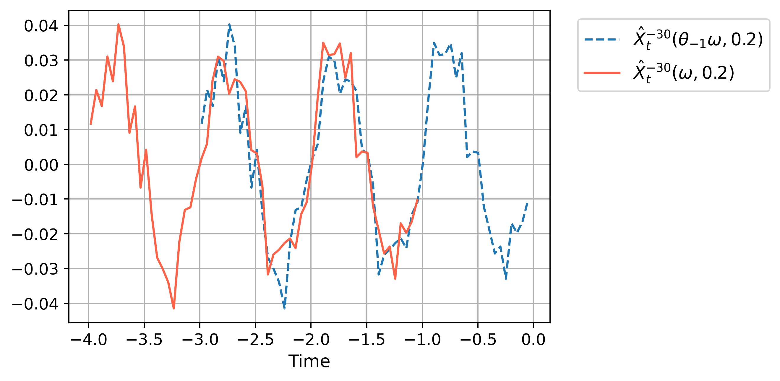
As discussed in [8], there are two ways to demonstrate the periodicity. The easer approach is to simulate the processes X^t∗​(ω)=Xt−30​(ω,0.2)\hat{X}_{t}^{*}(\omega)=X^{-30}_{t}(\omega,0.2)for t∈[−4,−1]t\in[-4,-1] and X^t∗​(θ−1​ω)=Xt−30​(θ−1​ω,0.2)\hat{X}_{t}^{*}(\theta_{-1}\omega)=X^{-30}_{t}(\theta_{-1}\omega,0.2) for t∈[−3,0]t\in[-3,0]. We can observe that the two segmented processes are identical in Figure 2 due to X^t−1∗​(ω)=X^t∗​(θ−1​ω)\hat{X}_{t-1}^{*}(\omega)=\hat{X}_{t}^{*}(\theta_{-1}\omega).

Refer to caption
Figure 2: Two paths with generated by backward Euler–Maruyama method on different realisations.
Refer to caption
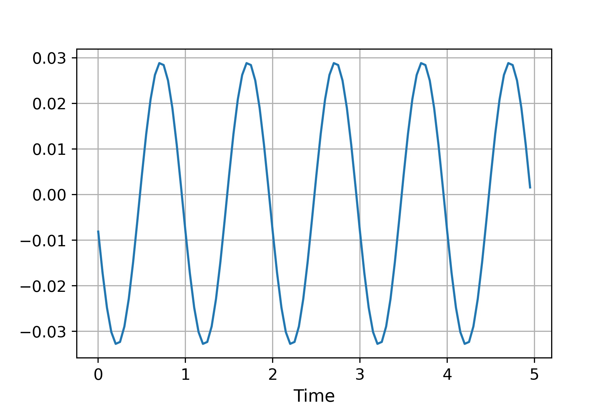
Figure 3: The pull-back path X^−30​(t,θ−t​ω)\hat{X}^{-30}(t,\theta_{-t}\omega) generated by backward Euler–Maruyama method.

The other way to check random periodicity of path XX with period τ\tau is to verify whether or not X^∗​(t,θ−t​ω)\hat{X}^{*}(t,\theta_{-t}\omega) is periodic with period τ\tau. To test it, we need to consider Xtt0​(θ−t​ω)X_{t}^{t_{0}}(\theta_{-t}\omega). Note that for any fixed r∈ℝr\in\mathbb{R} we have that

d​Xtt0​(θ−r​ω)=−10​π​Xtt0​(θ−r​ω)​d​t+sin⁡(2​π​t)​d​t+0.05​d​Wt​(θ−r​ω)=−10​π​Xtt0​(θ−r​ω)​d​t+sin⁡(2​π​t)​d​t+0.05​d​Wt−r.\displaystyle\begin{split}\mathrm{d}X_{t}^{t_{0}}(\theta_{-r}\omega)&=-10\pi X_{t}^{t_{0}}(\theta_{-r}\omega)\mathrm{d}t+\sin{(2\pi t)}\mathrm{d}t+0.05\mathrm{d}W_{t}(\theta_{-r}\omega)\\ &=-10\pi X_{t}^{t_{0}}(\theta_{-r}\omega)\mathrm{d}t+\sin{(2\pi t)}\mathrm{d}t+0.05\mathrm{d}W_{t-r}.\end{split} (37)

Now set t0=0t_{0}=0, and X00​(θ−r​ω)=x0X_{0}^{0}(\theta_{-r}\omega)=x_{0}. For each fixed rr, we simulate the path of Eqn. (37) through the backward Euler-Maruyama method up to t=rt=r. Then we obtain the evaluation of X^0​(r,θ−r​ω)\hat{X}^{0}(r,\theta_{-r}\omega). To allow convergence, we look at the path pattern from t=2t=2 to t=5t=5 in Figure 3. Apparently we have obtained a periodic pull-back path as expected, which in turn shows the random periodicity of the original path.

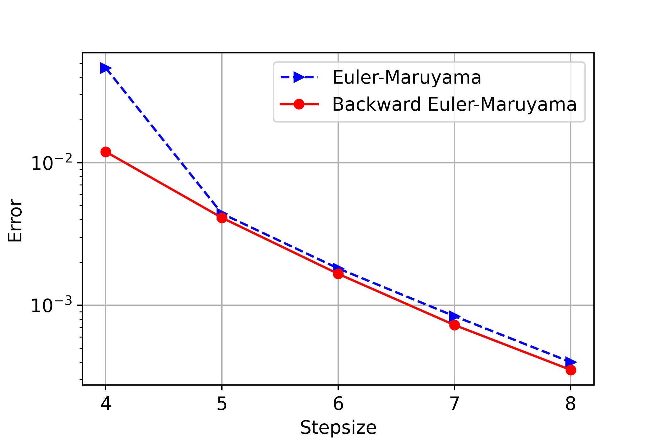
Finally, we test the order of convergence of the backward Euler-Maruyama method and compare the performance with (forward) Euler-Maruyama method. For its approximation we first generated a reference solution with a small step size of href=2−15h_{\text{ref}}=2^{-15}. This reference solution was then compared to numerical solutions with larger step sizes h∈{2−i:i=4,5,6,7,8}h\in\{2^{-i}:i=4,5,6,7,8\}. The error plot is shown in Figure 4. We plot the Monte Carlo estimates of the root-mean-squared errors versus the underlying temporal step size, i.e., the number i on the x-axis indicates the corresponding simulation is based on the temporal step size h=2−ih=2^{-i}. Both methods give the order of convergence above 11, which is beyond the theoretical order of convergence. When the stepsize is large, say, h=2−4h=2^{-4}, the Euler-Maruyama method has the error 0.048 which is almost five times of the error 0.011 from the backward Euler-Maruyama method. Indeed if we relax the stepsize to h=2−3h=2^{-3}, the Euler-Maruyama diverges while the backward Euler-Maruyama method still converges as expected. This further supports Theorem 1.2 and the advantage of backward Euler-Maruyama method: the backward Euler-Maruyama method converges regardless the size of stepsize (h<1h<1).

Refer to caption
Figure 4: Numerical experiment for simulating the random periodic solution of SDE (36): Step sizes versus L2L^{2} error.

Acknowledgements

This work is supported by the Alan Turing Institute for funding this work under EPSRC grant EP/N510129/1 and EPSRC for funding though the project EP/S026347/1, titled ’Unparameterised multi-modal data, high order signatures, and the mathematics of data science’. The author would also acknowledge Michael Scheutzow for useful discussion.

References

  • [1] L. Arnold, Random dynamical systems, 1995, Springer, Berlin, Heidelberg.
  • [2] W. J. Beyn, E. Isaak, and R. Kruse, Stochastic C-stability and B-consistency of explicit and implicit Euler-type schemes. Journal of Scientific Computing, 67.3(2016), pp.955-987.
  • [3] M. D. Chekroun, E. Simonnet and M. Ghil, Stochastic climate dynamics: random attractors and time-dependent invariant measures, Physica D, Vol.240 (2011), 1685-1700.
  • [4] A. Chojnowska-Michalik, Periodic distribution for linear equations with general additive noise, Bull. Pol. Acad. Sci Math., Vol.38 (1990), 23-33.
  • [5] G. Da Prato, P. Malliavin, D. Nualart, Compact families of Wiener functionals, C. R. Acad. Sci. Paris, Ser. I Math. Vol.351 (1992), 1287-1291.
  • [6] C. R. Feng and H. Z. Zhao, Random periodic solutions of SPDEs via integral equations and Wiener-Sobolev compact embedding, Journal of Functional Analysis, Vol.251(2011), 119-149.
  • [7] C. R. Feng and H. Z. Zhao, Random periodic processes, periodic measures and ergodicity. Journal of Differential Equations, 269.9(2020), 7382-7428.
  • [8] C. R. Feng, Y. Liu and H. Z. Zhao, Numerical approximation of random periodic solutions of stochastic differential equations, Zeitschrift für angewandte Mathematik und Physik, 68.5(2017), 1-32.
  • [9] C. R. Feng, Y. Luo and H. Z. Zhao, Random periodic solutions of stochastic functional differential equations, Doctoral dissertation, Loughborough University, 2014.
  • [10] C. R. Feng, Y. Wu and H. Z. Zhao, Anticipating random periodic solutions—I. SDEs with multiplicative linear noise, Journal of Functional Analysis, 271.2(2016), 365-417.
  • [11] C. R. Feng, Y. Wu and H. Z. Zhao, Anticipating Random Periodic Solutions–II. SPDEs with Multiplicative Linear Noise, ArXiv Preprint, arXiv:1803.00503.
  • [12] C. R. Feng, H. Z. Zhao and B. Zhou, Pathwise random periodic solutions of stochastic differential equations, Journal of Differential Equations, Vol.251(2011), 119-149.
  • [13] B. Gershgorin and A. J. Majda, A test model for fluctuation-dissipation theorems with time-periodic statistics, Physica D, Vol.239 (2010), 1741-1757.
  • [14] R. Z. Has’minskii, Stochastic Stability of Differential Equations, Sijthoff & Noordhoff, 1980.
  • [15] A. J. Majda and X. M. Wang, Linear response theory for statistical ensembles in complex systems with time-periodic forcing, Comm. Math. Sci., Vol.8 (2010), 145-172.
  • [16] J. M. Ortega and W. C. Rheinboldt, Iterative solution of nonlinear equations in several variables, volume 30 of Classics in Applied Mathematics, Society for Industrial and Applied Mathematics (SIAM), Philadelphia, PA, 2000. Reprint of the 1970 original.
  • [17] S. Riedel, and Y. Wu, Semi-implicit Taylor schemes for stiff rough differential equations, arXiv preprint, arXiv:2006.13689.
  • [18] M. Scheutzow, Periodic behaviour of the stochastic Brusselator in the mean-field limit, Probab. Th. Rel. Fields, Vol.72 (1986), 425-462.
  • [19] M. Scheutzow, and S. Schulze, Strong completeness and semi-flows for stochastic differential equations with monotone drift, Mathematical Analysis and Applications, 446.2.2017, 1555-1570.
  • [20] A. M. Stuart and A. R. Humphries, Dynamical Systems and Numerical Analysis, volume 2 of Cambridge Monographs on Applied and Computational Mathematics, Cambridge University Press, Cambridge, 1996.
  • [21] N. G. Van Kampen, Stochastic Processes in Physics and Chemistry, Elsevier, 2007.
  • [22] B. X. Wang, Existence, stability and bifurcation of random complete and periodic solutions of stochastic parabolic equations, J. Nonlinear Analysis, 103(2014), 9-25.
  • [23] G. Wanner, and E. Hairer, Solving ordinary differential equations II, Vol. 375 (1996). Springer Berlin Heidelberg.
  • [24] J. B. Weiss and E. Knobloch, A stochastic return map for stochastic differential equations, J. Stat. Phys., 58(1990),863-883.
  • [25] D. Willett and J.S.W. Wong, On the discrete analogues of some generalizations of Grönwall’s inequality, Monatshefte für Mathematik, 69.4 (1965), 362-367.
  • [26] A. Yevik, and H. Zhao, Numerical approximations to the stationary solutions of stochastic differential equations, SIAM journal on numerical analysis, 49.4.13 (2011), 97-1416.
  • [27] H. Z. Zhao and Z. H. Zheng, Random periodic solutions of random dynamical systems, J. Differential Equations, Vol.248(2009), 2020-2038.