Sparse recovery based on the generalized error function
Abstract
In this paper, we propose a novel sparse recovery method based on the generalized error function. The penalty function introduced involves both the shape and the scale parameters, making it very flexible. The theoretical analysis results in terms of the null space property, the spherical section property and the restricted invertibility factor are established for both constrained and unconstrained models. The practical algorithms via both the iteratively reweighted and the difference of convex functions algorithms are presented. Numerical experiments are conducted to illustrate the improvement provided by the proposed approach in various scenarios. Its practical application in magnetic resonance imaging (MRI) reconstruction is studied as well.
Keywords Sparse Recovery Generalized Error Function Nonconvex Regularization Iterative Reweighted L1 Difference of Convex functions Algorithms
1 Introduction
High dimensionality is a basic feature of big data, that is, the number of features measured can be very large and are often considerable larger than the number of observations. To overcome the "curse of dimensionality" and reduce the redundancy, the vector of parameters to be estimated or the signal to be recovered is often assumed to be sparse (i.e., it has only a few nonzero entries) either by itself or after a proper transformation. How to exploit the sparsity to help estimating the underlying vector of parameters or recovering the unknown signal of interest, namely sparse recovery, has become a core research issue and gained immense popularity in the past decades [1].
Generally, sparse recovery aims to estimate an unknown sparse from few noisy linear observations or measurements where with is the design or measurement matrix, and is the vector of noise. It arises in many scientific research fields including high-dimensional linear regression [2] and compressed sensing [3, 4, 5]. Naturally, this sparse can be recovered by solving a constrained -minimization problem
| (1) |
or the unconstrained -penalized least squares problem [6], where is a tuning parameter. However, due to the nonsmoothness and nonconvexity of the -norm, these are combinatorial problems which are known to be related to the selection of best subset and are computationally NP-hard to solve [7]. Instead, a widely used solver is the following constrained -minimization problem (also called Basis Pursuit Denoising) [3]:
| (2) |
or the well-known Lasso [8]. The -minimization acts as a convex relaxation of -minimization. Although it enjoys attractive theoretical properties and has achieved great success in practice, it is biased and suboptimal. The Lasso does not have the oracle property [9], since the -norm is just a loose approximation of the -norm.
To remedy this problem, many nonconvex sparse recovery methods have been employed to better approximate the -norm and enhance sparsity. They include () [10, 11, 12], Capped-L1 [13], transformed (TL1) [14], smooth clipped absolute deviation (SCAD) [9], minimax concave penalty (MCP) [15], exponential-type penalty (ETP) [16, 17], error function (ERF) method [18], [19, 20], [21], [22, 23], and -ratio sparsity minimization [24], among others. These parameterized nonconvex methods result in the difficulties of theoretical analysis and computational algorithms due to the nonconvexity of the penalty functions, but do outperform the convex -minimization in various scenarios. For example, it has been reported that gives superior results for incoherent measurement matrices, while , and -ratio sparsity minimization are better choices for highly coherent measurement matrices. Meanwhile, TL1 is a robust choice no matter whether the measurement matrix is coherent or not.
The resulting nonconvex sparse recovery methods have the following general constrained form:
| (3) |
where denotes a nonconvex penalty or regularization function with an approximation parameter (it can be a vector of parameters), or a formulation of its corresponding unconstrained version with being the tuning parameter. Several nonconvex methods and their corresponding penalty functions are shown in Table 1. Basically, in practice a separable and concave on penalty function is desired in order to facilitate the theoretical analysis and solving algorithms.
| Method | Penalty | Property |
|---|---|---|
| separable, concave on | ||
| Capped-L1 | ||
| TL1 | ||
| MCP | ||
| SCAD | ||
| ETP | ||
| ERF | ||
| nonseparable, nonconcave on | ||
| -ratio sparsity |
For the nonconvex methods mentioned above, there are a large number of theoretical recovery results for their global or local optimal solutions (please refer to the corresponding literature for a specific method). Moreover, some unified recovery analysis results have also been obtained for these nonconvex sparse recovery methods. For instance, [25] established a theoretical recovery guarantee through unified null space properties. A general theoretical framework was presented in [26] based on regularity conditions. It shows that under appropriate conditions, the global solution of concave regularization leads to desirable recovery performance and the global solution corresponds to the unique sparse local solution.
From an algorithmic point of view, many optimization algorithms have been used for solving the nonconvex problem (3) and its unconstrained version. Among them, [9] proposed a local quadratic approximation (LQA) for the SCAD method. A local linear approximation (LLA) was suggested in [27], which is a special case of the iteratively reweighted (IRL1) algorithm [28, 29]. The iterative reweighted algorithms were generalized in [30] to tackle a problem class of the sum of a convex function and a nondecreasing function applied to another convex function. In [13], a general framework of multi-stage convex relaxation was given, which iteratively refines the convex relaxation to achieve better solutions for nonconvex optimization problems. It includes previous approaches including LQA, LLA and the concave-convex procedure (CCCP) [31] as special cases. Under appropriate conditions, the author shows that the local solution obtained by the multi-stage convex relaxation method for nonconvex regularization achieves better recovery performance than the -regularization. In addition, the proximal gradient method [32] has also been extended to address the nonconvex problem (3). The ingredient of this method hinges on computing the proximal operator of the penalty function. It is well-known that the proximal operators of the -norm and the -norm are the hard-thresholding operator and the soft-thresholding operator, respectively. Most of nonconvex penalty functions also have proximal operators with closed-form. But for some penalty functions such as the ERF, there is no proximal operator with closed-form such that the corresponding proximal gradient method is inefficient in practice. Another general methodology that can be adopted to solve (3) and its unconstrained version is referred to the Difference of Convex functions Algorithms (DCA) [33, 34]. DCA reformulate the nonconvex penalty function as a difference of two convex functions and then solve it based on the DC programming, please see [35] for a comprehensive view of DCA approaches for sparse optimization.
1.1 Contribution
In this paper, we introduce a very flexible nonconvex sparse recovery method with the ETP and ERF approaches as special cases. We recognize that the generalized error function can be used to construct a smooth concave penalty function and provide a unified framework. The main contributions of the present paper are four-folds.
- (i)
We propose a general sparse recovery approach based on the generalized error function. The properties and the proximal operator of the proposed penalty are studied.
- (ii)
We establish a rigorous recovery analysis for the proposed approach in terms of the null space property, the spherical section property and the restricted invertibility factor for both constrained and unconstrained models.
- (iii)
We present efficient algorithms to solve the proposed method via both IRL1 and DCA, and carry out various numerical experiments to illustrate their superior performance.
- (iv)
We apply the proposed approach to magnetic resonance imaging (MRI) reconstruction, which improves the performance of state-of-the-art methods.
1.2 Related Work
The first study of the exponential-type penalty (ETP) was in the support vector machines problem [36]. Then this penalty together with its modifications was introduced into sparse regression [16], low-rank matrix recovery [37, 38] and sparse signal recovery [17]. Very recently, an approach based on the error function (ERF) has been proposed in [18] to promote sparsity for signal recovery. In comparison to these mostly related works, our main distinctions are summarized as follows:
- •
We have provided a fairly general framework of sparse recovery based on the generalized error function, making the existing ETP and ERF methods as its special cases.
- •
We have systematically studied the theoretical recovery analysis results and practical solving algorithms of our proposed method, while the existing literatures only contain part of our results. For instance, we have generalized the spherical section property based analysis in [17] from -bound to -bound for any . We have discussed the solving algorithms based on both IRL1 and DCA, while only IRL1 was considered in [18] for the ERF method.
- •
To the best of our knowledge, we are the first to adopt this kind of exponential-type approaches to MRI reconstruction.
1.3 Terminologies and Outline
We use the following terminologies throughout the paper. We denote vectors by lower bold case letters and matrices by upper case letters. Vectors are columns by defaults. denotes the -th component of the vector . is the sign function which is if and zero otherwise. We introduce the notations for the set and for the cardinality of a set in . We write for the complement of . For any vector , its "norm" is defined as for any , with the extension and . For a vector , we say is -sparse if at most of its entries are nonzero, i.e., if . denotes the vector which coincides with on the indices in and is extended to zero outside . denotes the support set of . For any matrix , the kernel of is defined as and denotes the submatrix with columns restricted to the index set . We use to denote the trace of a square matrix .
An outline of this paper is as follows. In Section 2, we introduce the proposed nonconvex sparse recovery method. We study the theoretical recovery analysis in Section 3. In Section 4, both the iteratively reweighted and the difference of convex functions algorithms are used to solve the nonconvex regularization problem. The proposed method adapted to the gradient for imaging applications is also discussed. In Section 5, a series of numerical experiments are conducted. Conclusions and some future works are presented in Section 6.
2 Proposed Method
We start with the definition of the generalized error function. For any , the generalized error function [39, 40] is defined as
| (4) |
Then, we have and (note that this is the standard error function). In addition, it is easy to verify that for any given , the generalized error function is concave on , strictly increasing with respect to , and . These properties can be observed from the function plots for the in with different choices of displayed in Figure 1.

Based on this generalized error function (GERF), for any and , we can use the following penalty function or regularization term for sparse recovery
| (5) |
where . Here is the shape parameter, while is the scale parameter. It is obvious that when , then and hence reduces to the -norm . The parameters and control the degree of concavity of the penalty function . We refer our proposed sparse recovery approach based on this penalty function as "GERF" throughout this paper. It is very flexible and includes some existing sparsity-promoting models as special cases. In particular, the exponential-type penalty (ETP) introduced in [16, 17] is the special case of , and the sparse recovery method based on the error function (referred as ERF) in [18] corresponds to the special case of .
In fact, regardless of some constant, our GERF penalty is an interpolation of the and penalty. It gains smoothness over the penalty and hence allows more computational options. Moreover, it improves the variable selection accuracy and achieves the oracle property by reducing the bias of the -minimization. The ability to choose suitable values of both the shape parameter and the scale parameter enables us to fully exploit its sparsity-promoting power and to achieve better recovery performance.
2.1 Properties of the Penalty
In what follows, we provide some useful properties for the functions and .
- •
The derivative of the function goes to
- •
is concave and non-decreasing in .
- •
According to the following double inequality given in [41]:
where , is a positive real number and
we are able to get the corresponding double inequality for .
- •
for any and .
- •
is concave on , that is for any and any , we have
- •
is sub-additive so that for any ,
And the additive property holds when have disjoint supports.
Next, we present a proposition that characterizes the asymptotic behaviors of with respect to and .
Proposition 1
For any nonzero , and ,
- (a)
It is trivial that , as .
- (b)
, as .
- (c)
, as . Moreover, if , then we have since .
Proof. With regard to (b), when , it holds that
where we let . When , it is obvious that .
As for (c), we have and ,
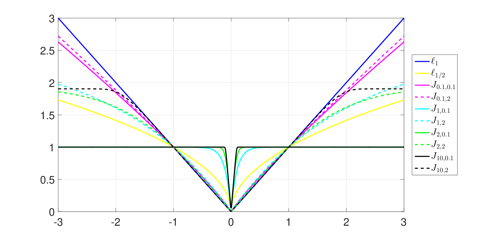
The objective functions of the GERF penalty in with various values of and are displayed in Figure 2. All the functions are scaled to attain the point for a better comparison. As shown, the proposed GERF model gives a good approximation to the penalty for a small value of , and approaches the penalty for a small value of or a large value of .
Moreover, we compare the GERF penalty functions ( and ) and their derivatives with other popular penalty functions in . From Figure 3, it can be seen that the GERF penalty functions have very similar patterns as other widely used penalty functions. Specifically, all the penalties displayed are concave, nondecreasing on , and are folded or near-folded (i.e., the functions become constant for large variable) [42]. Their derivatives are all nonincreasing, finite at , and equal to or close to zero when the variable of function is large, which satisfy the criterion for an unbiased penalty function that its derivative has a horizontal asymptote at zero. What stand out for our proposed GERF penalty are its smoothness and flexibility.

2.2 Proximal operator
In this subsection, we discuss the proximal operator for the GERF. For a function and a parameter , the proximal operator is defined as
| (6) |
As we know, the proximal operator for the -norm is the soft-thresholding operator , while the proximal operator for the -norm is the hard-thresholding operator . With regard to the GERF model, the proximal operator for the penalty function fulfills the optimality condition as follows:
Then, it is easy to observe that we have when , otherwise the minimizer is given as the solution of the following nonlinear equation:
In general, the solution has no closed-form but can be numerically found via the Newton’s method. It is worth mentioning that for the special case of (i.e., for the ETP method), a solution with closed-form as well as the corresponding proximal operator can be obtained by using the Lambert W function [43], please see the details in [17]. Here we present the proximal operators for the GERF with and in Figure 4 when is fixed to . As we can see, for a large , the proximal operators for the GERF are close to the soft-thresholding operator, whereas they are similar to the hard-thresholding operator for a small . These findings are largely consistent with earlier statements in Proposition 1.

3 Recovery Analysis
In this section, we set out to establish the theoretical recovery analysis for the proposed GERF approach. Both constrained and unconstrained models are considered.
3.1 Null Space Property
We begin with the null space property based analysis for the following noiseless constrained GERF minimization problem:
| (7) |
It is well-known that an exact sparse recovery can be guaranteed for the noiseless -minimization if and only if the measurement matrix satisfies a null space property (NSP) [44]:
| (8) |
Similarly, a generalized version of NSP guarantees an exact sparse recovery for our proposed GERF approach.
Definition 1
Given and , we say a matrix satisfies a generalized null space property (gNSP) relative to and if
| (9) |
It satisfies the gNSP of order relative to if it satisfies the gNSP relative to and any with
Then, based on the sub-additive property of the penalty function , it is straightforward to obtain the following theorem, which provides a sufficient and necessary condition for an exact sparse recovery via the GERF approach. Its proof follows almost the same as that given in Section 3.3 of [18] and so is omitted.
Theorem 1
For any given measurement matrix , and , every -sparse vector is the unique solution of the problem (7) if and only if satisfies the gNSP of order relative to .
We note that since the penalty function is separable and symmetric on , and concave on , the following result holds as an immediate consequence of Proposition 4.6 in [25], which verifies that our proposed GERF approach is superior to the -minimization in sparse uniform recovery.
Theorem 2
Let , with . Then we have
Consequently, the gNSP relative to is less demanding than the NSP for -minimization.
3.2 Spherical Section Property
Regarding the noiseless model (7), in this subsection we further show that by choosing a proper , one can obtain a solution arbitrarily close to the unique solution of -minimization via (7) when is fixed.
Definition 2
For any , we say the measurement matrix possesses the -spherical section property if holds for all . Hence, we have
| (10) |
Remark. The -spherical section property introduced here is a direct extension of -spherical section property studied in [17, 45] from to any . Based on this newly defined spherical section property, the results established in this subsection generalize the corresponding results in [17, 45].
Proposition 2
Suppose has the -spherical property for some . If , then is the unique solution of the following noiseless -minimization problem:
| (11) |
Proof. If there exists a vector () such that and . Then . Therefore, if holds for some , then we have
However, . Moreover, it holds that . As a result, we arise in a contradiction that
Hence, is the unique solution of the -minimization problem (11).
Lemma 1
Suppose has the -spherical section property for some . Let . Then for any subset such that , we have
| (12) |
Moreover, if has at most entries with absolute values greater than , then
| (13) |
where denotes the smallest integer greater than or equal to .
Proof. When , this lemma holds trivially since . Otherwise, when , it holds that
Meanwhile, , which completes the proof of (12).
To prove (13), we let be the indices of entries with absolute values not greater than , then . By using (12), we have
This proof is completed.
Lemma 2
Assume has the -spherical section property for some and . Then for any and , we have
| (14) |
whenever .
Proof. Assume denotes the indices of entries with absolute values greater than in . Note that
Meanwhile, , which yields such that . That is to say, there are at most entries of that have absolute values greater than . Furthermore, since , so at most entries of has absolute values that are greater than . Then the fact the and Lemma 1 complete the proof of this lemma.
Lemma 3
If is the solution of the problem (7) and the conditions in Lemma 2 hold, then it satisfies
Proof. Notice that
In addition, yields that . Therefore, the proof is completed.
Then, as a result of Lemma 2 and Lemma 3, the following theorem holds immediately.
3.3 Restricted Invertibility Factor
Next, we move on to discuss the recovery analysis result for the solution of the unconstrained or regularized version of GERF approach:
| (15) |
where with . Following the general theory of concave regularization presented in [26], our concave penalty has the form
| (16) |
where is the scalar regularization function.
Then the threshold level of this penalty , which is a function of that provides a normalization of , satisfies that . In what follows, based on the tools of restricted invertibility factor and null consistency condition used in [26], we are able to obtain an error bound for the GERF regularization method. For a rigorous proof of the main result, the reader is referred to [26] for detailed arguments.
Definition 3
([26]) For , and , the restricted invertibility factor (RIF) is defined as
| (17) |
Definition 4
Theorem 4
Assume and the -NC condition holds with some . Then for all , we have
| (19) |
4 Algorithms
In this section, we present the algorithms to solve the proposed GERF method via both IRL1 and DCA, and study the GERF on the gradient for imaging applications. We consider the following unconstrained problem:
| (20) |
where is the tuning parameter. Note that, in order to solve the constrained version of the GERF approach, we merely need to make some small modifications to the algorithms for solving the unconstrained model (20). For the sake of brevity of the article, we will not repeat the discussion for the constrained model.
4.1 IRL1
As discussed in [18, 30], an iteratively reweighted (IRL1) algorithm can be used to solve the nonsmooth nonconvex problem (20). At each iteration, this algorithm needs to solve a reweighted subproblem given as follows:
| (21) |
with weights . Then an alternating direction method of multipliers (ADMM) algorithm [46] can be adopted to solve this subproblem (21). We introduce an auxiliary vector and then consider the augmented Lagrangian
| (22) |
where is a small fixed positive parameter and is the dual variable. The ADMM algorithm is based on minimizing the augmented Lagrangian successively over and , and then applying a dual variable update to , which yields the following updates:
for iterations .
4.2 DCA
Another type of approaches that can be used to solve the nonsmooth nonconvex problem (20) is the Difference of Convex functions Algorithms (DCA) [33, 34], where we express the nonconvex penalty as a difference of two convex functions. With regard to our penalty , since
hence we have the following DC decomposition:
| (23) |
Then the problem (20) can be expressed as a DC program:
where and .
| (24) |
Note that, for each DCA iteration, it is required to solve the following -regularized subproblem:
| (25) |
Here we can also employ an ADMM algorithm to solve this subproblem by introducing an auxiliary vector and then considering the augmented Lagrangian
| (26) |
where is a small fixed positive parameter and is the dual variable. The resulting ADMM algorithm consists of the following updates:
for iterations .
4.3 GERF on the gradient
In this subsection, we discuss the imaging applications with a GERF minimization adapted to the gradient. Let be the image of interest, be the measurement matrix and be the measurements. For the MRI reconstruction, , where denotes the Fourier transform and is the sampling mask in the frequency space. We denote as the horizontal and vertical partial derivative operators respectively, and is the gradient operator in the discrete setting. Then, the reconstruction algorithm based on the GERF approach goes to
| (27) |
where . Let be the gradient vector at pixel , then can be rewritten as
| (28) |
Then we are able to use the framework of DCA proposed previously to solve this problem. In each DCA iteration, the subproblem reduces to a total variation (TV) [47] type of minimization, which can be handled efficiently by using the split Bregman technique [48]. In this paper, in order to solve (27) we directly adopt a simple modification of the Algorithm 2 in [49] (or Algorithm 3 in [20]), where a combination of DCA and split Bregman technique is used for the minimization adapted to the gradient. We are only required to replace the approximation vector in [49] by a new for our GERF approach. For the sake of conciseness, we will not reproduce the procedure for this algorithm. The reader is referred to [49] or [20] for details.
5 Numerical Experiments
In this section, we conduct a series of numerical experiments to demonstrate the advantageous performance of our proposed GERF method. Throughout this section, the support of -sparse signal is a random index set and its nonzero entries follow a standard normal distribution.
5.1 A Test with IRL1 and DCA
Firstly, we do a numerical test to compare the reconstruction performance of the proposed GERF approach by using the IRL1 and DCA algorithms with for a sparse signal reconstruction with a Gaussian random measurement matrix . Two cases are considered here, one is that the true signal has a sparsity level of and the measurements are noise free, while the other case is that the true signal is -sparse and the measurements are noisy with . We set and for the noise free and noisy cases, respectively. It can be observed from Figure 5 that in both cases the reconstructed signals via IRL1 and DCA methods are almost the same. The corresponding computing time for these two algorithms are listed in Table 2, which shows that the DCA is faster than the IRL1 in both cases. Therefore, we adopt the former throughout our numerical experiments to solve the problem (20).

| IRL1 | DCA | |
|---|---|---|
| Noise Free | 0.169 (0.098) | 0.118 (0.055) |
| Noisy | 0.144 (0.071) | 0.124 (0.067) |
5.2 Choice of Parameters
Next, we carry out a simulation study to understand the effects of the shape parameter and the scale parameter on recovering sparse signals based on the generalized error function. In this set of experiments, the true signal is of length and simulated as -sparse with in the set . The measurement matrix is a random matrix generated as Gaussian. For each and , we replicate the experiments times. It is recorded as one success if the relative error . We show the success rate over the replicates for various values of parameters and , while varying the sparsity level .
As shown in Figure 6, the proposed GERF method outperforms the -minimization (denoted as in the figure) for all tested values of and . It approaches the -minimization for a very small value of (see when ). In addition, it can be seen from Subfigure 6(a) that when is very small (e.g., ), the different choices of have very limited effect on the recovery performance. Looking at other Subfigures (6(b),6(c),6(d)), it is apparent that and are the best two choices for a moderate value of (e.g., ).
From Figure 7, we see that and are the best two among all tested values of when is fixed to , and . In contrast, when is set to be moderate large (e.g., ), the gap of the recovery performance becomes small for different values of . In this case, is the best among all tested values.


5.3 Algorithm Comparison
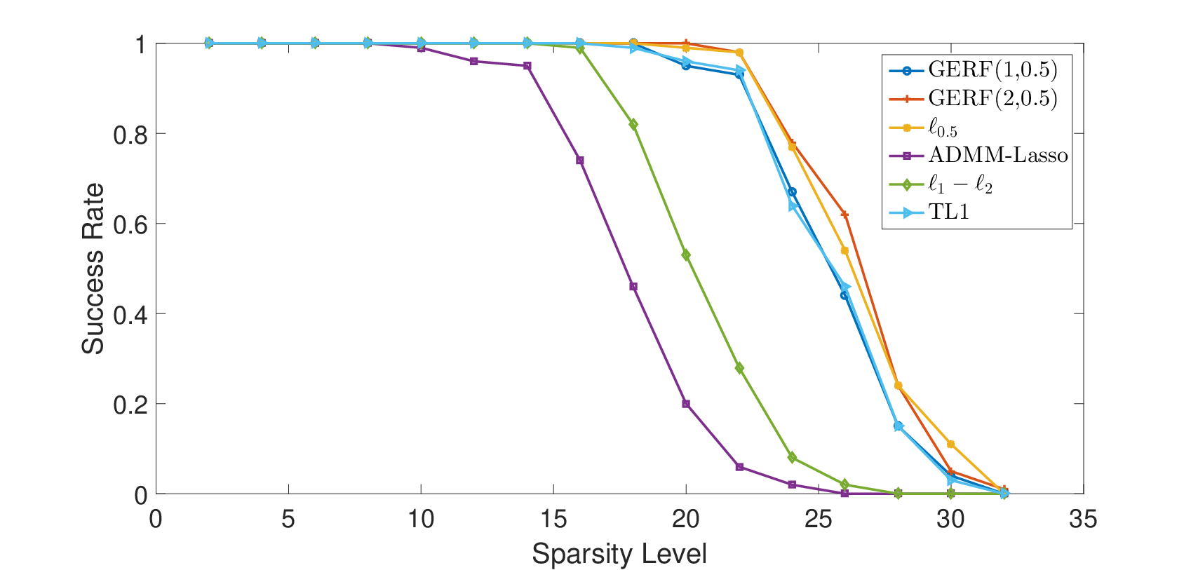
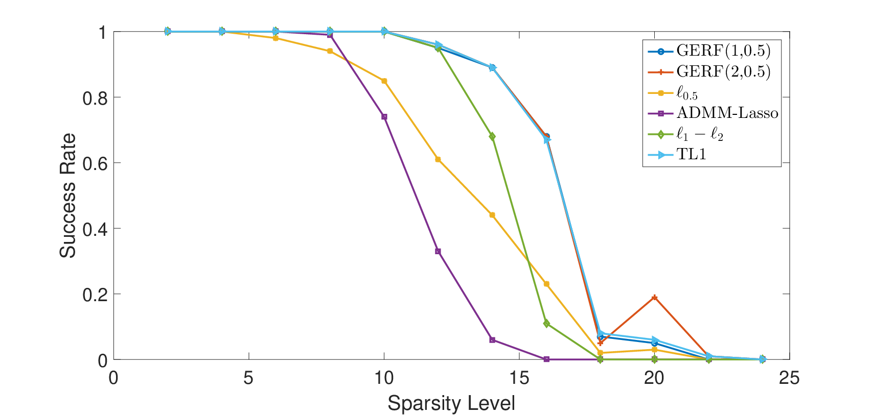
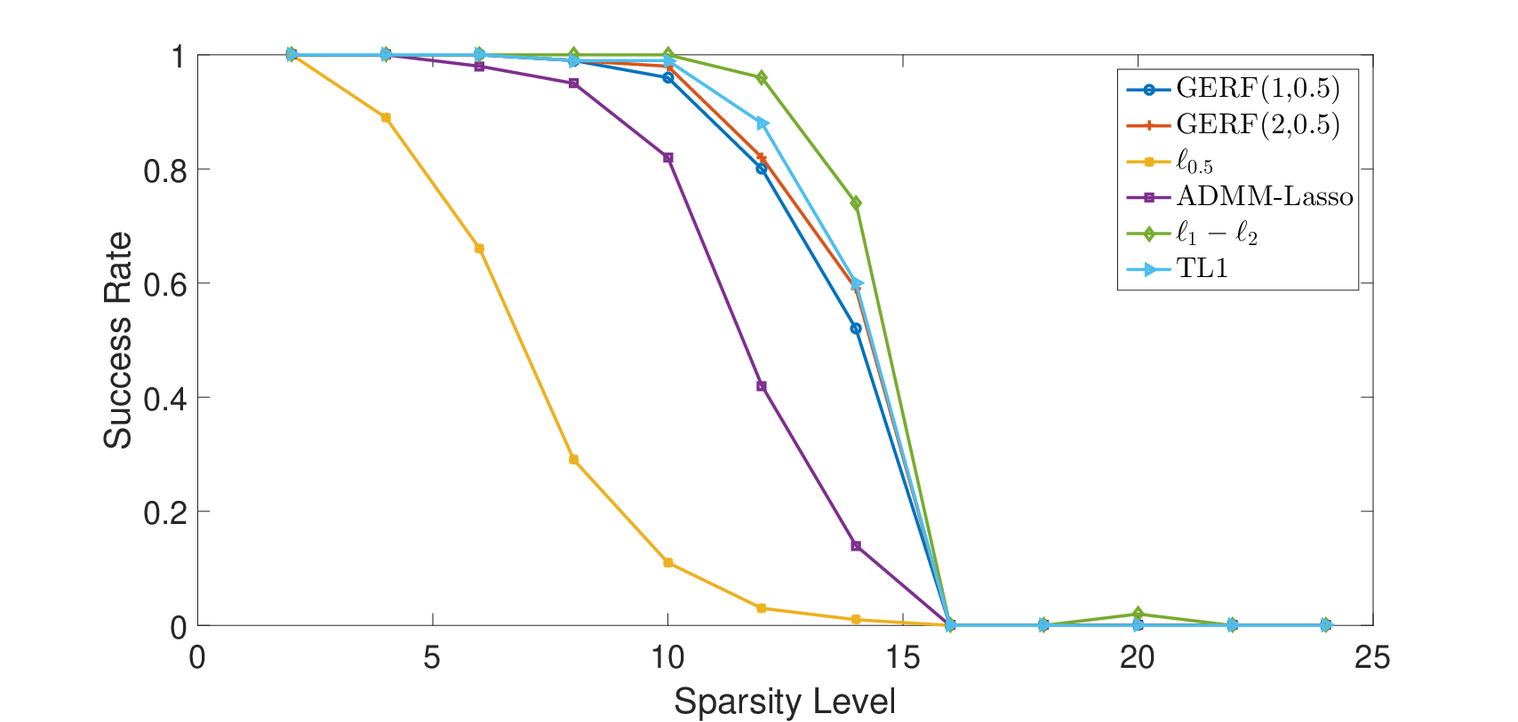
In this subsection, we compare the proposed GERF method with other state-of-the-art sparse recovery methods including ADMM-Lasso, , and TL1 (). In this set of experiments, we consider two scenarios for measurement matrices, i.e., Gaussian random matrix and oversampled discrete cosine transform (DCT) matrix. For the Gaussian random matrix, it is generated as a matrix with entries drawn from i.i.d. standard normal distribution. For the oversampled DCT matrix, we use with , and is a random vector uniformly distributed in . It is well-known that the DCT matrix is highly coherent and a larger yields a more coherent matrix.
Figure 8 shows that for the Gaussian case, the and the GERF with are the best two methods while our proposed GERF method with has an almost same performance as the TL1 method, which are the third best. They are all much better than the ADMM-Lasso and .
The corresponding results for the oversampled DCT matrix case are displayed in Figure 9. For these two coherent cases, we can observe that although the GERF is not the best, but it is still comparable to the best ones (the TL1 for and the for ). Thus, the GERF approach proposed in the present paper gives satisfactory and robust recovery results no matter whether the measurement matrix is coherent or not.
Furthermore, we present a simulation study for the noisy case. As done in [18], we consider to recover a -sparse signal of length from noisy Gaussian random measurements with Gaussian noise (zero mean and standard deviation ). The measurement matrix is of size with ranging from to . We evaluate the reconstruction performance in terms of the mean-square-error (MSE) over replications. The benchmark MSE of an oracle solution is computed as , where is the support of the ground-truth . In Figure 10, we compare the proposed GERF approaches ( and ) with the and the oracle solutions. As we can see, both of our proposed GERF solutions are very close to the oracle solution for large values of , while the solution is obviously biased.

5.4 MRI Reconstruction
Finally, we examine the particular application of the GERF approach on the gradient in MRI reconstruction. We use the Shepp-Logan phantom of size from radical projections without noise. We compare the reconstruction performance of the filtered back projection (FBP), total variation (TV), L1-L2 [20, 49] and our proposed GERF approach with , in terms of the relative error (RE) which equals to . As we can see from Figure 11, our proposed GERF approach achieves a near-perfect recovery using only projections, with a relative error , which is much better than the classical FBP, TV and L1-L2 methods.

6 Conclusion
In this paper, we proposed a concave sparse recovery approach based on the generalized error function, which is less biased than the approach. Theoretically, the recovery analysis was established for both constrained and unconstrained models. Computationally, both IRL1 and DCA algorithms are used to solve the nonsmooth nonconvex problem. A large number of numerical results demonstrated its advantageous performance over the state-of-the-art sparse recovery methods in various scenarios. The MRI phantom image reconstruction test also indicated its superior performance.
In future work, the extensions to structured sparsity (e.g., block sparse recovery and the matrix analogues) are of immense interest. Other practical imaging applications including image denoising and image deblurring should be explored as well.
References
- [1] Trevor Hastie, Robert Tibshirani, and Martin Wainwright. Statistical learning with sparsity: the lasso and generalizations. CRC press, 2015.
- [2] Peter Bühlmann and Sara Van De Geer. Statistics for high-dimensional data: methods, theory and applications. Springer Science & Business Media, 2011.
- [3] David L Donoho. Compressed sensing. IEEE Transactions on Information Theory, 52(4):1289–1306, 2006.
- [4] Yonina C Eldar and Gitta Kutyniok. Compressed sensing: theory and applications. Cambridge University Press, 2012.
- [5] Simon Foucart and Holger Rauhut. A Mathematical Introduction to Compressive Sensing, volume 1. Birkhäuser Basel, 2013.
- [6] Rahul Mazumder, Jerome H Friedman, and Trevor Hastie. Sparsenet: Coordinate descent with nonconvex penalties. Journal of the American Statistical Association, 106(495):1125–1138, 2011.
- [7] Balas Kausik Natarajan. Sparse approximate solutions to linear systems. SIAM Journal on Computing, 24(2):227–234, 1995.
- [8] Robert Tibshirani. Regression shrinkage and selection via the lasso. Journal of the Royal Statistical Society: Series B (Methodological), 58(1):267–288, 1996.
- [9] Jianqing Fan and Runze Li. Variable selection via nonconcave penalized likelihood and its oracle properties. Journal of the American Statistical Association, 96(456):1348–1360, 2001.
- [10] Rick Chartrand and Wotao Yin. Iteratively reweighted algorithms for compressive sensing. In Acoustics, speech and signal processing, 2008. ICASSP 2008. IEEE international conference on, pages 3869–3872. IEEE, 2008.
- [11] Rick Chartrand and Valentina Staneva. Restricted isometry properties and nonconvex compressive sensing. Inverse Problems, 24(3):035020, 2008.
- [12] Simon Foucart and Ming-Jun Lai. Sparsest solutions of underdetermined linear systems via -minimization for . Applied and Computational Harmonic Analysis, 26(3):395–407, 2009.
- [13] Tong Zhang. Analysis of multi-stage convex relaxation for sparse regularization. Journal of Machine Learning Research, 11(3), 2010.
- [14] Shuai Zhang and Jack Xin. Minimization of transformed penalty: theory, difference of convex function algorithm, and robust application in compressed sensing. Mathematical Programming, 169(1):307–336, 2018.
- [15] Cun-Hui Zhang. Nearly unbiased variable selection under minimax concave penalty. Annals of Statistics, 38(2):894–942, 2010.
- [16] Cuixia Gao, Naiyan Wang, Qi Yu, and Zhihua Zhang. A feasible nonconvex relaxation approach to feature selection. In Proceedings of the AAAI Conference on Artificial Intelligence, volume 25, 2011.
- [17] Mohammadreza Malek-Mohammadi, Ali Koochakzadeh, Massoud Babaie-Zadeh, Magnus Jansson, and Cristian R Rojas. Successive concave sparsity approximation for compressed sensing. IEEE Transactions on Signal Processing, 64(21):5657–5671, 2016.
- [18] Weihong Guo, Yifei Lou, Jing Qin, and Ming Yan. A novel regularization based on the error function for sparse recovery. arXiv preprint arXiv:2007.02784, 2020.
- [19] Yifei Lou and Ming Yan. Fast L1–L2 minimization via a proximal operator. Journal of Scientific Computing, 74(2):767–785, 2018.
- [20] Penghang Yin, Yifei Lou, Qi He, and Jack Xin. Minimization of for compressed sensing. SIAM Journal on Scientific Computing, 37(1):A536–A563, 2015.
- [21] Zhiyong Zhou and Jun Yu. A new nonconvex sparse recovery method for compressive sensing. Frontiers in Applied Mathematics and Statistics, 5:14, 2019.
- [22] Yaghoub Rahimi, Chao Wang, Hongbo Dong, and Yifei Lou. A scale-invariant approach for sparse signal recovery. SIAM Journal on Scientific Computing, 41(6):A3649–A3672, 2019.
- [23] Chao Wang, Ming Yan, Yaghoub Rahimi, and Yifei Lou. Accelerated schemes for the minimization. IEEE Transactions on Signal Processing, 68:2660–2669, 2020.
- [24] Zhiyong Zhou and Jun Yu. Minimization of the -ratio sparsity with for signal recovery. arXiv preprint arXiv:2010.03402, 2020.
- [25] Hoang Tran and Clayton Webster. A class of null space conditions for sparse recovery via nonconvex, non-separable minimizations. Results in Applied Mathematics, 3:100011, 2019.
- [26] Cun-Hui Zhang and Tong Zhang. A general theory of concave regularization for high-dimensional sparse estimation problems. Statistical Science, 27(4):576–593, 2012.
- [27] Hui Zou and Runze Li. One-step sparse estimates in nonconcave penalized likelihood models. Annals of statistics, 36(4):1509, 2008.
- [28] Emmanuel J Candes, Michael B Wakin, and Stephen P Boyd. Enhancing sparsity by reweighted minimization. Journal of Fourier Analysis and Applications, 14(5-6):877–905, 2008.
- [29] Yun-Bin Zhao and Duan Li. Reweighted -minimization for sparse solutions to underdetermined linear systems. SIAM Journal on Optimization, 22(3):1065–1088, 2012.
- [30] Peter Ochs, Alexey Dosovitskiy, Thomas Brox, and Thomas Pock. On iteratively reweighted algorithms for nonsmooth nonconvex optimization in computer vision. SIAM Journal on Imaging Sciences, 8(1):331–372, 2015.
- [31] Alan L Yuille and Anand Rangarajan. The concave-convex procedure. Neural Computation, 15(4):915–936, 2003.
- [32] Neal Parikh and Stephen Boyd. Proximal algorithms. Foundations and Trends in optimization, 1(3):127–239, 2014.
- [33] Pham Dinh Tao and Le Thi Hoai An. Convex analysis approach to dc programming: theory, algorithms and applications. Acta Mathematica Vietnamica, 22(1):289–355, 1997.
- [34] Pham Dinh Tao and Le Thi Hoai An. A dc optimization algorithm for solving the trust-region subproblem. SIAM Journal on Optimization, 8(2):476–505, 1998.
- [35] Hoai An Le Thi, T Pham Dinh, Hoai Minh Le, and Xuan Thanh Vo. Dc approximation approaches for sparse optimization. European Journal of Operational Research, 244(1):26–46, 2015.
- [36] Paul S Bradley and Olvi L Mangasarian. Feature selection via concave minimization and support vector machines. In ICML, volume 98, pages 82–90. Citeseer, 1998.
- [37] Mohammadreza Malek-Mohammadi, Massoud Babaie-Zadeh, Arash Amini, and Christian Jutten. Recovery of low-rank matrices under affine constraints via a smoothed rank function. IEEE Transactions on Signal Processing, 62(4):981–992, 2013.
- [38] Mohammadreza Malek-Mohammadi, Massoud Babaie-Zadeh, and Mikael Skoglund. Iterative concave rank approximation for recovering low-rank matrices. IEEE Transactions on Signal Processing, 62(20):5213–5226, 2014.
- [39] Li Yin and Feng Qi. Some functional inequalities for generalized error function. Journal of Computational Analysis and Applications, 25(7):1366–1372, 2018.
- [40] Jianjun Wang, Feng Zhang, Jianwen Huang, Wendong Wang, and Changan Yuan. A nonconvex penalty function with integral convolution approximation for compressed sensing. Signal Processing, 158:116–128, 2019.
- [41] Horst Alzer. On some inequalities for the incomplete gamma function. Mathematics of Computation, 66(218):771–778, 1997.
- [42] Hongcheng Liu, Tao Yao, Runze Li, and Yinyu Ye. Folded concave penalized sparse linear regression: sparsity, statistical performance, and algorithmic theory for local solutions. Mathematical Programming, 166(1-2):207–240, 2017.
- [43] Robert M Corless, Gaston H Gonnet, David EG Hare, David J Jeffrey, and Donald E Knuth. On the LambertW function. Advances in Computational Mathematics, 5(1):329–359, 1996.
- [44] Albert Cohen, Wolfgang Dahmen, and Ronald DeVore. Compressed sensing and best -term approximation. Journal of the American Mathematical Society, 22(1):211–231, 2009.
- [45] Yin Zhang. Theory of compressive sensing via -minimization: A non-rip analysis and extensions. Journal of the Operations Research Society of China, 1(1):79–105, 2013.
- [46] Stephen Boyd, Neal Parikh, and Eric Chu. Distributed optimization and statistical learning via the alternating direction method of multipliers. Now Publishers Inc, 2011.
- [47] Leonid I Rudin, Stanley Osher, and Emad Fatemi. Nonlinear total variation based noise removal algorithms. Physica D: nonlinear phenomena, 60(1-4):259–268, 1992.
- [48] Tom Goldstein and Stanley Osher. The split Bregman method for L1-regularized problems. SIAM Journal on Imaging Sciences, 2(2):323–343, 2009.
- [49] Yifei Lou, Tieyong Zeng, Stanley Osher, and Jack Xin. A weighted difference of anisotropic and isotropic total variation model for image processing. SIAM Journal on Imaging Sciences, 8(3):1798–1823, 2015.