Line Marching Algorithm For Planar Kinematic Swarm Robots: A Dynamic Leader-Follower Approach

Though each individual in a swarm is always subject to limited sensing, computing, decision and execution capability, the swarm as a whole exhibits marvelous performance. For example, by working in groups, the ant colony can move food hundreds of times heavier than their weights, thereby improving the foraging efficiency of the population [1]. Another typical example is the formation flying of geese, which helps to reduce energy expenditure and thus increase migration distance [2]. Inspired by the biological behaviors of social animals, formation control has received extensive attention which gives rise to a significant amount of research results revealing the underlying mechanism of the biological behaviors. In addition, formation control is also appealing from the perspective of engineering applications, such as cooperative searching, exploration, escort and commercial performance[3, 4, 5].

Roughly speaking, there are two main classes of control approaches to solving the formation control problem. The first class is the virtual structure approach [6, 7, 8, 9, 10, 11, 12], which treats formation as a single entity, and the formation is maintained by keeping the relative position between a virtual leader and each agent. Early works establishing the virtual structure approach can be found in [6, 7]. Since after, the virtual structure approach has been advanced in several directions, such as dealing with system nonlinearity [8], integration with learning based approach [9], and adaptation to unreliable communication network [10], just to name a few. Recently, a simulated annealing algorithm was proposed by [11] featuring optimal multiphase homing tracking trajectory and a novel formation guidance strategy in order to reduce the impact caused by the unpredictable environment. [12] proposed a formation control strategy for UAVs, where the formation control problem was decomposed into the smooth trajectory generation problem and the trajectory tracking problem. With the help of the super-twisting method, the airflow influences between UAVs can be compensated effectively when performing formation flying missions. A salient advantage of the virtual structure approach lies in that it makes it easy to define, maintain and keep formation. However, since the definition of formation is label-specified, once an agent fails, the formation will be incomplete unless further re-organization is made. As a result, the virtual structure approach is not robust or flexible enough in the face of agent failures.

The second class is the leader-follower approach [13, 14, 15, 16, 17, 18, 19, 20, 21], which decouples the formation control problem into a set of leader-following tracking problem. By specifying a chain of leader-follower pair, formation can be achieved by the regulation of relative position and direction of each leader-follower pair. Seminal works for the leader-follower approach can be found in [13, 14], which lay the foundation for various important extensions. For example, [15] considered input constraint; [16] adopted a receding-horizon scheme in the expect of fast exponential convergence; [17] considered the fixed-time convergence issue; [18] took into account dynamic optimization; [19] studied distance-based formation. Recently, in the absence of global position and direction measurement, [20] proposed a flexible formation approach to track multiple mobile robots based on estimated relative position. Likely, by utilizing relative velocity and bearing measurements, a distributed control approach was synthesized by [21] which guaranteed a desired geometric pattern for the agents under persistent exciting condition. Due to the simple design philosophy, the leader-follower approach is easy to understand and implement in practice. While, since the order of the chain of leader-follower pairs in the existing results are fixed, once an agent fails, the other agents subsequential to the failed agent in the chain will be greatly affected, which makes the traditional leader-follower approach vulnerable to agent failures.

As mentioned above, it is difficult for both the virtual structure approach and the traditional leader-follower approach to deal with agent failures. The reason behind this is these approaches are fully label-specified, i.e., the desired position for each agent in the formation is uniquely determined by its label. To address this issue, in this paper, we further propose a dynamic leader-follower approach to solving the line marching problem for a swarm of planar kinematic robots. In contrast to the existing results, the desired positions for the robots in the line are not fully label-specified, but determined in a dynamic way according to the current state of the robot swarm. By constantly forming a chain of leader-follower pairs, exact formation can be achieved by pairwise leader-following tracking. Since the order of the chain of leader-follower pairs is constantly updated, the proposed algorithm shows strong robustness against robot failures. In particular, once a robot fails, the rest robots will re-form a new chain of leader-follower pairs and form a new marching line. The failed robot will be considered as an obstacle by other robots. After the failed robot gets back to normal, it will rejoin the swarm and the whole robot swarm will re-form, again, into a new line and keep marching forward.

The following notation are adopted in this paper. Let $\mathbb{R}$ and $\mathbb{N}$ denote the sets of real numbers and positive integers, respectively. Given $x\in\mathbb{N}$,

Given angle $\theta$, the rotation matrix is defined as

Given $x,y\in\mathbb{R}^{2}$, the inner product of $x$ and $y$ is denoted by $\langle x,y\rangle$. The boolean relation “or” is denoted by $\vee$. Given a nonzero vector $x\in\mathbb{R}^{2}$, let $\gamma(x)=x/||x||$ denote the unit vector which has the same direction as $x$.

In this paper, we consider a swarm of $N$ planar kinematic robots moving in an unbounded region subject to $M$ immobile or mobile obstacles. Throughout this paper, it is assumed that the positions of all the robots and obstacles are expressed in a common coordinate system.

For $i\in\underline{N}$, the motion of the $i$th robot is described by the following equation:

where $p_{i}(t),v_{i}(t)\in\mathbb{R}^{2}$ denote the position and velocity vector of the $i$th robot, respectively.

Let $\delta_{i}>0$ denote the minimal safety distance for the $i$th robot.

For $i\in\underline{M}$, the motion of the $i$th obstacle is described by the following equation:

where $q_{i}(t),u_{i}(t)\in\mathbb{R}^{2}$ denote the position and velocity vector of the $i$th obstacle, respectively. For immobile obstacles, $u_{i}(t)=0$ for all $t\geq 0$.

Let $\nu_{i}>0$ denote the minimal safety distance for the $i$th obstacle.

Roughly speaking, as illustrated by Fig. 1, the task for the robots is to march in a line while keep collision avoidance for both obstacles and other robots. Let $v_{l}\in\mathbb{R}^{2}$ denote the nonzero marching velocity, and $e_{l}=\gamma(v_{l})$ denote the marching direction. Then, let $e_{l}^{\perp}=\mathbf{R}(\pi/2)e_{l}$ denote the orientation vector perpendicular to $e_{l}$ by rotating $e_{l}$ anticlockwise by $90$ degree. Mathematically, the task considered in this paper can be described as follows:

• •

  collision avoidance

  1. 1.

     for all $t\geq 0$, for all $i,j\in\underline{N}$, $i\neq j$,

     $$||p_{i}(t)-p_{j}(t)||\geq\delta_{i}+\delta_{j}.$$

     (3)

  2. 2.

     for all $t\geq 0$, for all $i\in\underline{N}$, $j\in\underline{M}$,

     $$||p_{i}(t)-q_{j}(t)||\geq\delta_{i}+\nu_{j}.$$

     (4)

• •

  line marching

  1. 1.

     for all $i\in\underline{N}$,

     $$\lim_{t\rightarrow\infty}(v_{i}(t)-v_{l})=0.$$

     (5)

  2. 2.

     for all $i,j\in\underline{N}$, $i\neq j$,

     $$\lim_{t\rightarrow\infty}\langle p_{i}(t)-p_{j}(t),e_{l}^{\perp}\rangle=0.$$

     (6)

  3. 3.

     there exists an order $(i_{1},i_{2},\dots,i_{N})$ where $i_{k}\in\underline{N}$ such that for $k\in\underline{N-1}$,

     $$\lim_{t\rightarrow\infty}\langle p_{i_{k+1}}(t)-p_{i_{k}}(t),e_{l}\rangle=\rho$$

     (7)

     where $\rho>0$ denotes the desired inter-robot distance.

To avoid the possible conflict between collision avoidance and line marching, $\rho$ should be chosen such that for all $i,j\in\underline{N}$, $i\neq j$,

Equation (7) indicates that the order of the marching line is immaterial as long as the relative position of the robots in the line can be maintained, which makes it possible that, when some robots fail, the rest robots can re-form a new marching line.

In this paper, we propose a novel dynamic leader-follower approach for the task of robots line marching. The basic idea is to form a chain of leader-follower pairs in a self-organized way in the sense that the order of the chain shall not be uniquely specified by the label of the robots, but rather determined by the current state of the robot swarm.

In this section, we consider a swarm of $10$ planar kinematic robots. The parameters for the line marching are given by $v_{l}=(-8,12)^{T}\triangleq(v_{lx},v_{ly})^{T}$, $\rho=4$. For simplicity, the minimal inter-robot safety distance is set to be $\delta_{i}\triangleq\delta=1$. The control parameters are selected to be $\kappa_{1}=1.5$, $\kappa_{2}=10$, $a_{i}=10$, $\omega_{i}=1$, $\alpha=10$, $\beta=10$. In the following, we will consider two cases for numerical simulation.

In this section, we apply the proposed line marching algorithm to discrete-time model. In this case, equations (1) and (2) become

and

respectively, where $T>0$ denotes the sampling time. Note that the discrete-time versions of $v_{i,ca}(t)$ and $v_{i,lm}^{j}(t)$ by (15) and (17) are straightforward and thus are omitted.

The line marching algorithm for the discrete-time case is given by Algorithm 2. In what follows, we use Python to obtain the simulation results.

In this section, we also consider a swarm of $10$ planar kinematic robots. The parameters for the line marching are given by $v_{l}=(-8,12)^{T}$, $\rho=4$. The sampling time is chosen to be $T=0.001$. The minimal inter-robot safety distance is set to be $\delta_{i}\triangleq\delta=1$. The control parameters are selected to be $\kappa_{1}=1.5$, $\kappa_{2}=10$, $a_{i}=10$, $\omega_{i}=1$, $\alpha=10$, $\beta=10$.

We consider the line formation subject to a mobile obstacle with $\nu_{1}=10$ and $u_{1}(t)=(15,0)^{T}$. The initial positions of the robots are give by $p_{1}(0)=(-5,10)^{T}$, $p_{2}(0)=(1,20)^{T}$, $p_{3}(0)=(-10,5)^{T}$, $p_{4}(0)=(5,10)^{T}$, $p_{5}(0)=(10,5)^{T}$, $p_{6}(0)=(0,10)^{T}$, $p_{7}(0)=(5,-10)^{T}$, $p_{8}(0)=(15,-5)^{T}$, $p_{9}(0)=(-5,-10)^{T}$, $p_{10}(0)=(-10,-5)^{T}$. The initial position for the obstacle is given by $q_{1}(0)=(-80,60)^{T}$.

In the following simulation, we consider four phases:

1. 1.

   from $k=0$ to $k=3000$, the robots will form a line from the initial position;

2. 2.

   from $k=3000$ to $k=8000$, the robots will bypass the mobile obstacle and re-form a marching line;

3. 3.

   from $k=8000$ to $k=11000$, robot 4 fails;

4. 4.

   from $k=11000$ to $k=15000$, robot 4 gets back to normal and rejoins the robot swarm.

Fig. 9 shows the robots’ and mobile obstacle’s positions during the whole simulation process. It can be seen that the robot swarm has firstly managed to form a marching line, and then successfully bypassed the mobile obstacle. When robot 4 fails, other robots consider robot 4 as an immobile obstacle and has re-formed a new marching line. After robot 4 gets back to normal, it rejoins the marching line, which happens to be at the same position before the event of failure.

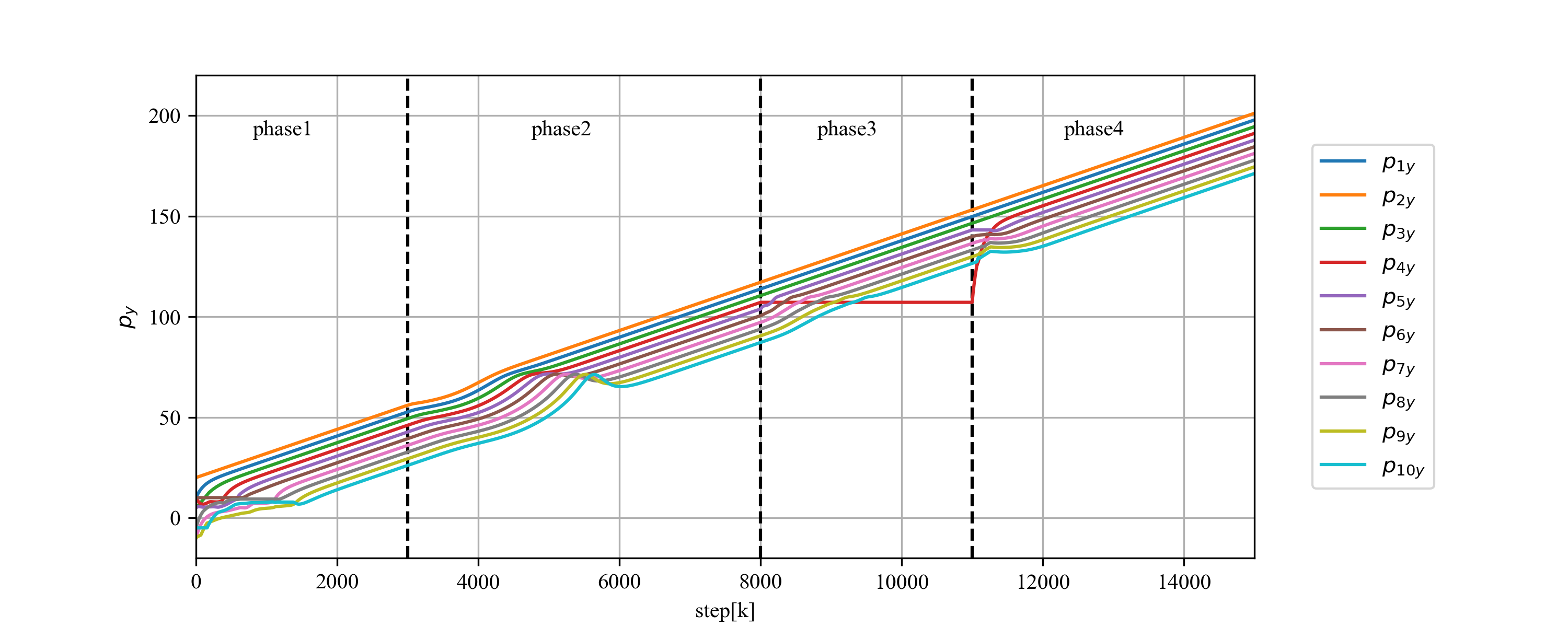
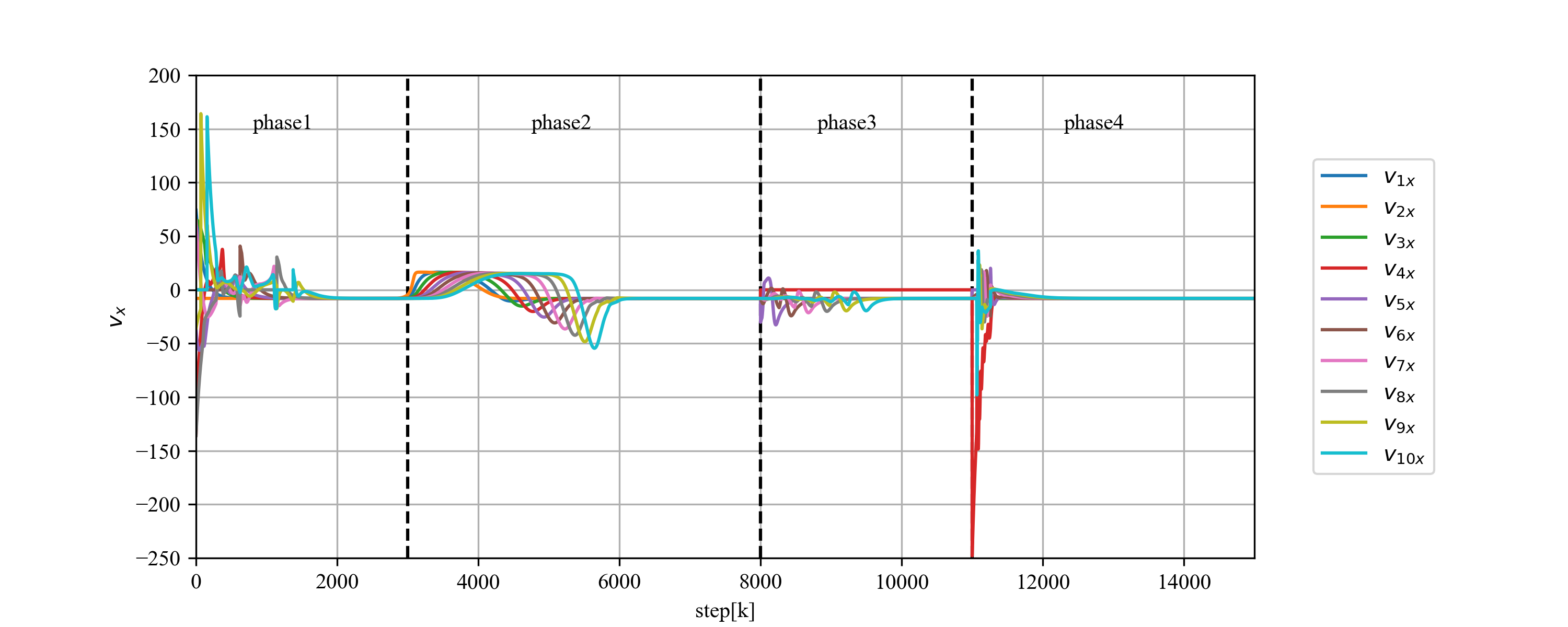
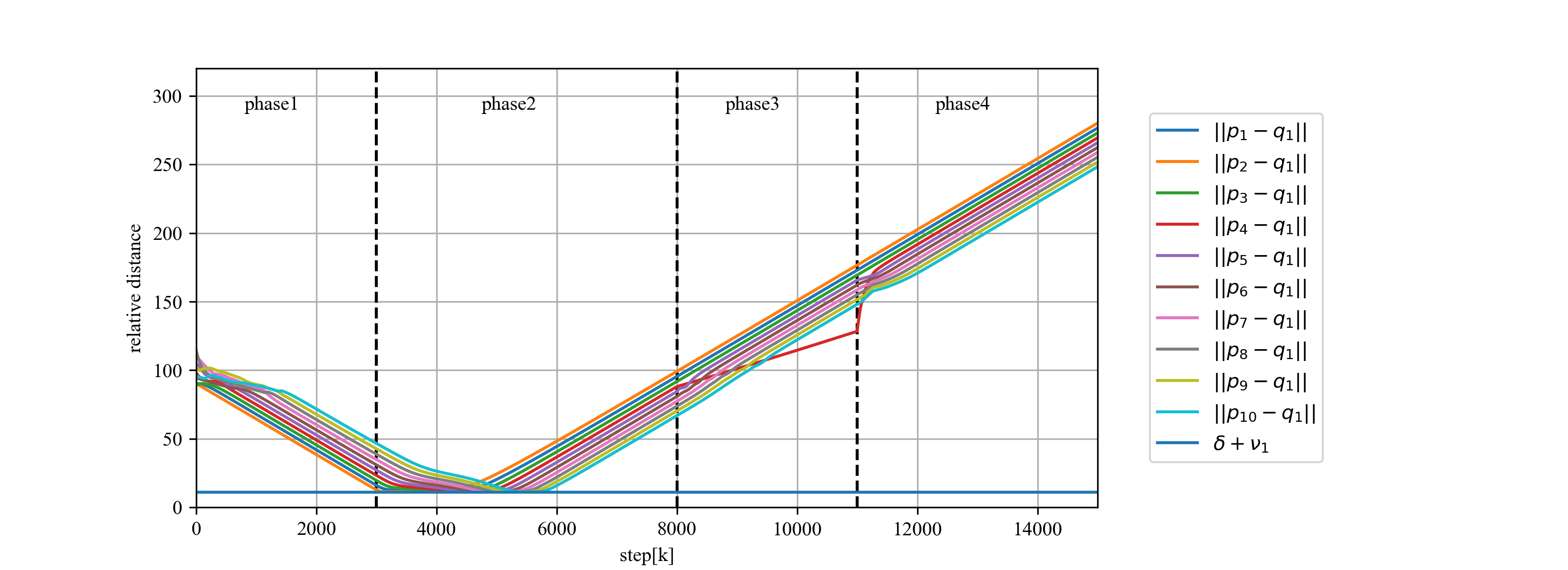
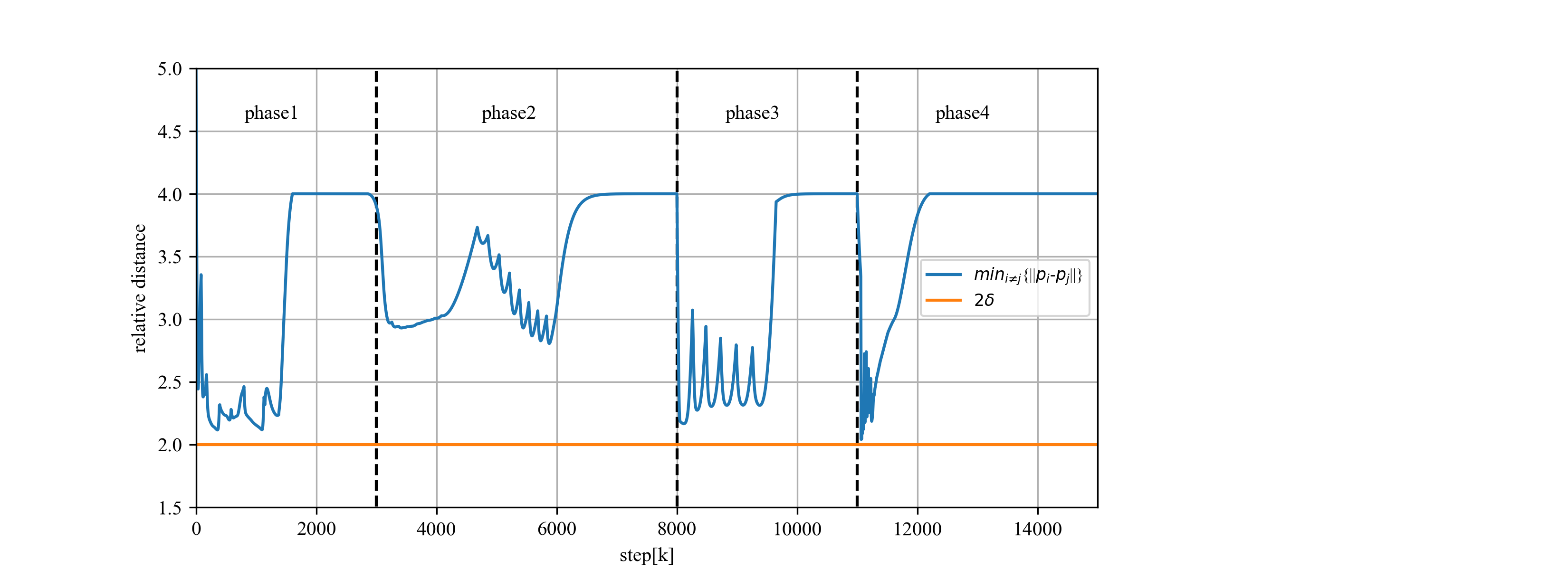
Figs. 10 and 11 show the time profiles of the robots’ positions and velocities, respectively. It can be seen that the line marching objective has been successfully achieved. Fig. 12 shows the relative distance between each robot and the mobile obstacle, and the minimal relative distance between two robots, which indicates no collision as expected.

In this section, we consider the more practical situation where the robot is described by the unicycle model, and the numerical simulation is performed on the ROS platform. In particular, for $i\in\underline{N}$, the kinematic equations of the $i$th robot are given by

where $p_{i}(t)\in\mathbb{R}^{2}$, $\vartheta_{i}(t)\in\mathbb{R}$ denote the position and heading angle of the $i$th robot, respectively, and $\upsilon_{i}(t)\in\mathbb{R}$, $\varpi_{i}(t)\in\mathbb{R}$ denote the linear and angular velocity, respectively.

Let $l_{i}$ denote the distance between the wheel pair of the $i$th robot, and then

denote the speeds of left wheel and the right wheel of the robot, respectively. Since the system (20) is nonlinear, the proposed line marching algorithm cannot be applied directly. To tackle this issue, we perform the following coordinate transformation as in [22]:

where $d_{i}>0$ is some small number. Then it follows that

Let

and

Then, we have

Moreover, it can be verified that for all $t\geq 0$, $\Theta_{i}(t)$ is nonsingular whose inverse is given by

By using the coordinate transformation (22), the nonlinear system (20) is transformed into a linear kinematic system (23), which is in the same form of (1) and thus the proposed algorithm is applicable. After obtaining $\bar{v}_{i}(t)$, the linear and angular velocity inputs to system (20) are given by

and then the speeds of left and right wheel of the robot can be determined by equation (21).

Note that in ROS platform, the position measurements of the robots are subject to the Gaussian noise. As a result, the co-leader situation would almost be impossible. Thus, Algorithm 1 can be further simplified into Algorithm 3. For ROS simulation, the robot moves continuously with respect to time. While, to implement the algorithm in a decentralized way, it takes time for inter-robot communication. Thus, the desired velocities for the robot swarm will be updated periodically with $T$ denoting the period.

Different from the cases studied in Sections 4 and 5, in ROS simulation, the linear and angular velocities of the robots are subject to saturation. For $i\in\underline{N}$, suppose $|\upsilon_{i}(t)|\leq\upsilon_{\max}$, $|\varpi_{i}(t)|\leq\omega_{\max}$.

Similar to the cases studied in Sections 4 and 5, we consider a swarm of 10 robots. Let $T=0.02\mathrm{s}$. The parameters for the line marching are given by $v_{l}=(-0.25,0.433)^{T}$, $\rho=2$. For simplicity, the minimal inter-robot safety distance is set to be $\delta_{i}\triangleq\delta=0.35$. Suppose $\upsilon_{\max}=1\mathrm{m/s}$, $\omega_{\max}=2\mathrm{rad/s}$. The control parameters are selected to be $\kappa_{1}=2.5$, $\kappa_{2}=10$, $a_{i}=10$, $\omega_{i}=0.3$, $\alpha=1$, $\beta=0.5$, $d_{i}=0.2$. Suppose there is a mobile obstacle with $\nu_{1}=2$ and $u_{1}(t)=(0.2133,0.211)^{T}$.

The initial positions of the robots are given by $p_{1}(0)=(-4,8)$, $p_{2}(0)=(0,12)$, $p_{3}(0)=(-8,4)$, $p_{4}(0)=(4,8)$, $p_{5}(0)=(8,4)$, $p_{6}(0)=(0,8)$, $p_{7}(0)=(4,-8)$, $p_{8}(0)=(12,-4)$, $p_{9}(0)=(-4,-8)$, $p_{10}(0)=(-8,-4)$. The initial heading angles are given by $\vartheta_{i}(0)=0$. The initial position for the obstacle is given by $q_{1}(0)=(-30,23)^{T}$.

Similar to the case studied in Section 5, the whole simulation process is divided into four phases:

1. 1.

   from $t=0$s to $t=54$s, the robots will form a line from the initial position;

2. 2.

   from $t=54$s to $t=130$s, the robots will bypass the mobile obstacle and re-form a marching line;

3. 3.

   from $t=130$s to $t=160$s, robot 6 fails;

4. 4.

   from $t=160$s to $t=218.8$s, robot 6 gets back to normal and rejoins the robot swarm.

Figs. 13-16 show the positions of the robot swarm and the obstacle during each phase, respectively. Similar to the simulation results in Section 5, it can be observed that both the line marching objective and the collision avoidance objective have been achieved. Moreover, the algorithm proves to be robust against robot failure. Figs. 17 and 18 show the time profiles of robots’ positions and velocities, respectively. Fig. 19 shows the relative distance between each robot and the mobile obstacle, and the minimal relative distance between two robots. These simulation results further confirm the effectiveness of the proposed algorithm.

This paper proposed a dynamic leader-follower approach to solving the line marching problem for a swarm of planar kinematic robots. In contrast to the existing exact formation algorithms, such as the virtual structure approach or the traditional leader-follower approach, the proposed approach shows strong robustness against robot failure by constantly updating the chain of leader-follower pairs. Comprehensive numerical results using Matlab, Python and ROS are provided to validate the effectiveness of the proposed algorithm for continuous-time, discrete-time and unicycle systems, respectively.

This work was supported in part by National Natural Science Foundation of China under Grant [grant number 61773170, 61703167], and in part by Guangdong Nature Science Foundation under [grant number 2021A1515012584].

References

- [1] M. Dorigo, M. Birattari and T. Stutzle, “Ant colony optimization,” IEEE Computational Intelligence Magazine., 1(4): 28-39, 2006.
- [2] C. M. Bishop, R. J. Spivey, P. J. Butler, etal, “The roller coaster flight strategy of bar-headed geese conserves energy during Himalayan migrations,” Science., 347(6219):250-254, 2015.
- [3] X. Dong, Formation and Containment Control for High-order Linear Swarm Systems., Springer-Verlag Berlin Heidelberg, 2016.
- [4] H. Liu and B. Zhu, Formation Control of Multiple Autonomous Vehicle Systems., John Wiley & Sons, 2018.
- [5] H. Ahn, Formation Control: Approaches for Distributed Agents., Springer Nature Switzerland AG, 2020.
- [6] M. A. Lewis, K.-H. Tan, “High precision formation control of mobile robots using virtual structures,” Autonomous Robots, 4(4):387–403, 1997.
- [7] M. Egerstedt, M. Hu, “Formation constrained multi-agent control,” IEEE Transactions on Robotics and Automation, 17(6):947–951, 2001.
- [8] Do, K. D., Pan, J, “Nonlinear formation control of unicycle-type mobile robots,” Robotics and Autonomous Systems, 55(3):191-204, 2007.
- [9] Y. Liu, Y. Jia, An iterative learning approach to formation control of multi-agent systems, Systems & Control Letters, 61(1):148–154, 2012.
- [10] X. Dong and G. Hu, Time-varying formation control for general linear multi-agent systems with switching directed topologies, Automatica, 73:47-55, 2016.
- [11] Q. Chen, Y. Sun, M. Zhao and M. Liu, “A Virtual Structure Formation Guidance Strategy for Multi-Parafoil Systems,” IEEE Access, 7:123592-123603, 2019.
- [12] Z. Li and B. Xian, “Robust distributed formation control of multiple unmanned aerial vehicles based on virtual structure,” Control Theory & Applications, 37(11):2423-2431, 2020.
- [13] J. P. Desai, J. P. Ostrowski, V. Kumar, “Modeling and control of formations of nonholonomic mobile robots,” IEEE Transactions on Robotics and Automation, 17(6):905-908, 2001.
- [14] A. K. Das, R. Fierro, V. Kumar, J. P. Ostrowski, J. Spletzer and C. J. Taylor, “A vision-based formation control framework,” IEEE Transactions on Robotics and Automation, 18(5):813-825, 2002.
- [15] L. Consolini, F. Morbidi, D. Prattichizzo and M. Tosques, “Leader-follower formation control of nonholonomic mobile robots with input constraints,” Automatica, 44(5):1343-1349, 2008.
- [16] J. Chen, D. Sun, J. Yang, H. Chen, “A leader-follower formation control of multiple nonholonomic mobile robots incorporating receding-horizon scheme,” The International Journal of Robotics Research, 29(6):727-747, 2010.
- [17] Z. Gao and G. Guo, “Fixed-Time Leader-Follower Formation Control of Autonomous Underwater Vehicles With Event-Triggered Intermittent Communications,” IEEE Access, 6:27902-27911, 2018.
- [18] H. Xiao and C. L. P. Chen, “Leader-Follower Consensus Multi-Robot Formation Control Using Neurodynamic-Optimization-Based Nonlinear Model Predictive Control,” IEEE Access, 7:43581-43590, 2019.
- [19] C. L. P. Chen, D. Yu and L. Liu, “Automatic Leader-Follower Persistent Formation Control for Autonomous Surface Vehicles,” IEEE Access, 7:12146-12155, 2019.
- [20] Y. Wang, M. Shan, Y. Yue and D. Wang, “Vision-Based Flexible Leader- Follower Formation Tracking of Multiple Nonholonomic Mobile Robots in Unknown Obstacle Environments,” IEEE Transactions on Control Systems Technology, 28(3) :1025-1033, 2020.
- [21] Z. Tang, R. Cunha, T. Hamel and C. Silvestre, “Formation control of a leader-follower structure in three dimensional space using bearing measurements,” Automatica, 128:567-573, 2021.
- [22] W. Ren and E. Atkins, “Distributed multi-vehicle coordinated control via local information exchange”, International Journal of Robust and Nonlinear Control, 17(10-11):1002-1033.