DESY 21–079
HU-EP 21/13
BHLS2 Upgrade : spectra, muon HVP
and the [] System
The generic Hidden Local Symmetry (HLS) model has recently given rise to its BHLS2 variant, defined by introducing symmetry breaking mostly in the vector meson sector; the central mechanism is a modification of the covariant derivative at the root of the HLS approach. However, the description of the dipion spectra, especially the Belle one, is not fully satisfactory whereas the simultaneous dealing with its annihilation sector () is optimum. We show that this issue is solved by means of an additional breaking term which also allows to consistently include the mixing properties of the system within this extended BHLS2 (EBHLS2) scope. This mechanism, an extension of the usual ’t Hooft determinant term, only affects the kinetic energy part of the BHLS2 Lagrangian. One thus obtains a fair account for the dipion spectra which complements the fair account of the annihilation channels already reached. The Belle dipion spectrum is found to provide evidence in favor of a violation of CVC in the lepton decay; this evidence is enforced by imposing the conditions on EBHLS2 axial current matrix elements. EBHLS2 is found to recover the usual (completed) formulae for the [] mixing parameters and the global fits return mixing parameter values in agreement with expectations and better uncertainties. Updating the muon HVP, one also argues that the strong tension between the KLOE and BaBar pion form factors imposes to provide two solutions : and , in units of , rather than some combination of these. Taking into account common systematics, their differences with the experimental BNL-FNAL average value exhibit significances (KLOE) and (BaBar) with fit probabilities favoring the former.
1 Introduction
The Standard Model provides the accepted framework which embodies the strong, electromagnetic and weak interactions; it accounts accurately for the observable values reported from low energies up to the highest ones reached at the LHC. A very few specific measurements look, however, borderline enough to rise a hint of a physics beyond the Standard Model. Among these, the very precisely measured muon anomalous magnetic moment plays a special role; it has generated – and still generates – an important experimental and theoretical activity related with its measurement by the E821 Experiment at BNL [1] , for its latest update; this value is at variance with expectations by to , depending on the various predictions, essentially differing by their estimates of the leading order hadronic vacuum polarisation (HVP-LO) as reported in [2] and displayed therein in Figure 44.
Actually, the significance just quoted refers to using HVP-LO evaluations derived by means of various Dispersion Relation (DR) methods. In contrast, the Lattice QCD (LQCD) Collaboration BMW [3] recently published an estimate for the HVP-LO [3] claiming a 0.8% precision and very close to what is needed to match the BNL measurement; accordingly, the BMW HVP-LO is at variance by more than with any of the reported DR evaluations of the HVP-LO.
The Muon Experiment running at FNAL has very recently published its first results [4] and found them in excellent accord with the previous BNL measurement [1]; the consistency of these two measurements allowing for their combination, the experimental reference value becomes :
Compared to the BNL measurement, this weighted average provides a noticeably improved uncertainty (30% reduction) and a downward shift by . This value still favors numerically the BMW estimate [3] for the HVP-LO over any of the DR ones.
Hence, the puzzle which was ”DR versus Data” may become 11 1 One should remind that based evaluations of the muon HVP may not be in contradiction with the BMW estimate as can be seen in the recent [5] (see also [2] for previous evaluations). This, however, supposes that the significant Isospin breaking mechanisms involved in the pion form factor in the decay and in annihilations – which can well differ – have all been clearly identified. This is one of the issues addressed in this article. ”DR versus LQCD” for which some different kind of physics beyond the Standard Model could have to be invoked. Indeed, if the HVP-LO as derived by DR methods provides a good global EW fit, the change suggested by the BMW evaluation severely impacts the goodness of the global EW fit [6], except if the changes can be localized at low enough energy – Reference [6] quotes 1.94 GeV, assuming the change in the cross-sections to be a mere global rescaling.
As long as the missing piece may spread out across the whole non-perturbative region of QCD which, as shown by the KEDR data [7], does not extend much above GeV, one has at hand a somewhat large lever arm. However, the recent KMPS study [8] has shown that the missing contribution to the HVP-LO should come from the energy region below GeV to accomodate the global EW fit. This locates the requested missing part of the annihilation cross-section to a very limited energy region widely explored by several independent groups having collected data using different detectors and colliders; this missing hadronic cross-section piece is expected to contribute an additional to the muon HVP-LO, larger than the light-by-light (LbL) contribution to the HVP.
Thus, the energy region to scrutinize is located well inside the realm of the Effective Resonance Lagrangian Aproaches (RLA) which have extended the scope of the Chiral Perturbation Theory (ChPT). The inclusion of resonances has given rise to the Resonance Chiral Perturbation Theory (RPT) formulation and to the Hidden Local Symmetry (HLS) Model which have been proved equivalent [9, 10]. Beside other processes, the HLS Model [11] encompasses the non-anomalous annihilation channels ; it can be complemented by its anomalous sector [12] which allows to also cover the annihilation channels. Because it deals with only the lowest lying resonance nonet, the validity range of the HLS Lagrangian naturally extends up to the mass region and is thus quite appropriate to explore the faulty energy region in accordance with QCD which is at the root of the different RLA.
As the BMW evaluation of the muon HVP-LO questions the annihilation data in the energy region up to the meson mass, it is worthwhile testing our understanding of its physics by means of such RLA, in particular the HLS model, which allows to explore this region already well covered by a large number of data samples in all the significant channels and thus shrink the window of possibilities to find a non negligible missing .
As the original HLS model22 2 See [13] for a comprehensive review covering the anomalous and non-anomalous sectors. assumes U(3) symmetry in both the vector (V) and pseudoscalar (P or PS) sectors, it should obviously be complemented by symmetry breaking inputs in order to account for the rich amount of data samples it is supposed to cover. A first release named BHLS [14, 15] essentially based on the BKY breaking mechanism [16, 17], extended [18] to account for Isospin breaking effects, was proven to perform satisfactorily; however, it exhibited some difficulty to manage with the threshold and regions for resp. the dipion and the 3 pion annihilation channels. In order to solve this issue, the breaking procedure has been deeply revisited and gave rise to BHLS2 under two variants [19] named respectively the Basic Solution (BS) and the Reference Solution (RS). Both BHLS2 variants are derived by complementing the BKY breaking mechanisms at work in the and sectors of the non-anomalous HLS Lagrangian by additional breaking schemes affecting solely the vector meson fields.
Regarding the vector sector of the BHLS2 BS variant, the new breaking input -- named Covariant Derivative (CD) Breaking -- turns out to perform the substitution33 3 To avoid lengthy repetitions, we refer the reader to the companion paper [19] for details. The present study is essentially an extension of BHLS2 which endorses its content, particularly its vector sector. in the covariant derivative which is a fundamental ingredient of the HLS model; the aim of is to break the symmetry for the components along the basis matrices , and of the canonical Gell-Mann algebra. The rule naturally propagates to the anomalous sector – i.e. the and Lagrangian pieces44 4 As one assumes the FKTUY [12] intrinsic parameters and to be equal, couplings ( being the electromagnetic field) identically vanish..
Regarding the PS sector of the BS variant of BHLS2 : Besides the BKY breaking associated with the part of the non–anomalous Lagrangian, the symmetry has been reduced by including the so–called ’t Hooft determinant term [20]; for our purpose, this turns out to add the singlet term to the kinetic energy of the PS fields.
However, if this canceled out the difficulties met at the dipion threshold and in the mass region, the account for the dipion spectra collected in the decay was not fully satisfactory as can be seen in Table 3 of [19] (see also the discussion in Section 17 herein); a closer look indicated that it is the description of the high statistics Belle sample [21] which is faulty. This issue was circumvented by introducing an additional breaking mechanism (the Primordial Mixing) which defines the RS Solution.
The original aim of the present study is to reexamine the issue actually raised by the dipion spectra and to figure out which kind of breaking can solve the problem met by the BS variant of BHLS2. In order to motivate this new breaking scheme – a generalization of the usual ’t Hooft determinant term – Section 3 proceeds to a thorough study of the various dipion spectra and of their impact on the other channels involved in the BHLS2 framework, especially on the pion form factor in the timelike and spacelike regions.
Once motivated, this extended breaking scheme is precisely defined and analyzed in Sections 4 and 5. The purpose of Section 6 is to address the modifications generated in the non–anomalous BHLS2 Lagrangian derived in [19] by this newly introduced kinetic breaking. Special emphasis is on the pion form factor involved in the decay of the lepton compared to its partner in annihilations ; it is shown that, while is still fulfilled55 5 Under conditions on discussed in Sections 4 and 7 of [19]., the CVC assumption is violated in the sector as . As the ALEPH [22] and Cleo [23] spectra accomodate easily a modelling with either of the and constraints, this result emphasizes the interest of having another dipion spectrum with a statististics comparable to those of Belle [21] or larger.
However, allowing for a violation of CVC within BHLS2 cannot be solely localized in the sector of the BHLS2 Lagrangian and it propagates to the anomalous Lagrangian pieces as noted in Section 7 and developped in the various Appendices. Hence, the description of processes as important as the annihilations is deeply modified and so should be tested versus data, as well as the decay modes and those involving couplings.
Prior to this exercise, our set of reference data samples has to be updated to account for new data samples [24, 25] or updated ones [26, 27]. This is done in two steps. First, the purpose of Section 8 is to deal with the newly issued three pion data sample collected by the BESIII Collaboration [24]. It is shown that the BESIII spectrum energies should be appropriately recalibrated to match the common energy scale of the other data samples included in our reference data set, especially in the and peak locations.
On the other hand, dealing with the dipion spectra is of course an important – and controversial – issue because of the long standing discrepancy between some of the available high statistics data samples. Therefore, we take profit of the newly published SND dipion spectrum [25] to revisit in Section 9 the consistency analysis of the different dipion samples to illustrate the full picture and motivate the way we deal with strong tensions when evaluating physics quantities of importance, especially the muon HVP-LO.
Having updated our reference set of data samples, Section 10 reports on global fits performed under various conditions, updating the results derived with the BS and RS variants of the former version of BHLS2 and those obtained using the extended formulation which is the subject of the present study; this extension will be named EBHLS2 for clarity. Section 11 addresses a key topic of the broken HLS model within the EBHLS2 context. Indeed, the question of supposedly uncontrolled uncertainties associated with using fit results based on an Effective Lagrangian may cast some shadow on this kind of methods. To definitely address this issue, the best is to quantify the effect by comparing the estimates for the muon HVP derived from EBHLS2 with those derived using more traditional methods under similar conditions. Subsection 11.1 illustrates for the dipion contribution to the muon HVP that specific biases attributable to using EBHLS2 are negligible compared to i/ the way the systematics, especially the normalization uncertainty of the various spectra, are dealt with by the various authors, ii/ the sample content used to derive one’s estimates. These two major sources of uncertainty are, on the other hand, common to any of the reported evaluations.
With these conclusions at hand, our evaluations of the muon HVP-LO are derived. Our favored result which excludes from the fit the dipion spectra from KLOE08 [28] and BaBar [29, 30] is examined in Subsection 11.2; an alternative solution where all KLOE data samples are discarded in favor of the BaBar one is also presented in Subsection 11.5. The full HVP-LO is constructed (Subsection 11.4) and compared with the other currently reported evaluations in Subsection 11.6.
Equiped with the kinetic breaking mechanism defined in Subsection 4.2, EBHLS2 is well suited to address the mixing properties of the system more precisely than was done with a similar – but much less sophisticated – modelling in [31]. The final aim is to rely on the results of the EBHLS2 fit over the largest set of data samples ever used to derive the corresponding mixing parameter values with optimum accuracy.
The derivation of the axial currents is the subject of Section 13. Section 14 addresses the singlet-octet basis parametrization defined by Kaiser and Leutwyler [32, 33, 34]; it is shown that EBHLS2 allows to recover the expected Extended ChPT relations. In Section 15, a similar exercise is performed within the quark flavor basis developped by Feldmann, Kroll and Stech (FKS) in [35, 36, 37] and one also yields the expected results. This clearly represents a valuable piece of information about the dealing of EBHLS2 in its PS sector.
The aim of Sections 16 and 17 is to push EBHLS2 a step further : One focuses on how Isospin symmetry breaking shows up in the axial currents associated to light quark pairs when expressed in terms of PS bare fields – a leading order approximation. The Kroll Conditions [38] :
are then examined in detail and shown to exhibit – at in breakings – unexpected constraints among the various components of the kinetic breaking term. In particular, satisfying the Kroll Conditions implies that a kinetic breaking with solely a term is not consistent and should be extended in order to involve and quadratic contributions. Whether this property is inherent to only EBHLS2 may look unlikely.
In Section 18, one reports on additional EBHLS2 fits suggested by the Kroll Conditions and tabulates the fit parameter values. The short Section 19 reports on side consequences on some physics parameters, especially the muon HVP-LO. Sections 20 and 21 report on the numerical evaluation of the mixing parameters and compare with available results from other groups.
Finally, Section 22 collects the conclusions of this work, an almost 100% COVID19 lockdown work.
2 Preamble : On the Free Parameters of the BHLS2 Model
Significant (anti-)correlations between , and the specific HLS parameter have been reported in our study [19]; this topic was the purpose of its Subsection 20.1. As parameter correlations may easily be of pure numerical origin66 6 For instance, the coefficients of the subtraction polynomial of any given loop function, may undergo significant correlations in minimization procedures; they are accounted for in the parameter error covariance matrix returned by the fits., we did not go beyond analyzing the issue numerically but emphasized that the physics conclusions were safe, i.e. not shadowed by these correlations.
Actually, one can go a step further. Indeed, it can be remarked that the three parameters , and are involved only in the piece of the non–anomalous BHLS2 Lagrangian and do not occur in its anomalous FKTUY pieces [12, 13]. Let us consider the pieces inherited from named here and in [19] and and perform therein the following parameter redefinition :
| (1) |
where and are introduced by the breaking matrix affecting which actually writes in the BHLS2 framework77 7 Note the missing square root symbol in the definition for given in [19]..
One can then check that the dependency upon drops out everywhere except in the mass term shown in the Lagrangian piece (see Equation (40) below). Obviously, this mass term has no influence on the phenomenology we address and thus is discarded.
It follows herefrom that the actual values for , and are in fact out of reach and that the single quantities which can be accessed using the data are their , combinations. Practically, fitting within the BHLS2 framework – having fixed – reduces the parameter freedom and the parameter correlations without any loss in the physics insight, being understood that the derived and are nothing but and just defined.
On the other hand, specific parameters are involved in order to deal with the system. They come from the transformation leading from the renormalized fields – those which diagonalize the PS kinetic energy term – to the physically observable states and can be found88 8 See also Subsection 4.3 in [14]. in Section 5. These parameters have been named , and in accordance with the usual custom [35, 38].
In our previous works on the HLS model, in particular [14, 19], one of the () mixing angles [32, 33] has been constrained () following a former study [31]. This turns out to impose the mixing angle be algebraically related to the BKY parameter and the nonet symmetry breaking parameter (see Subsection 4.4 in [14]). The experimental picture having dramatically changed since [31], this assumption deserves certainly to be revisited as will be done in the present work. Moreover, we also imposed [39] :
| (2) |
As a whole, this lessens the number of free parameters by 2 units without any degradation of the fit quality or any change in the HVP values.
However, for the present purpose, it has been found worthwhile to release these constraints and let , and vary freely. When analyzing below the mixing properties, this assumption will be revisited in a wider context.
3 Revisiting the Dipion Spectra : A Puzzle?
Section 17 of [19] reported the properties of our set of – more than 50 – data samples when submitted to global fits based on either of the Reference Solution (RS) and Basic Solution (BS) variants of the BHLS2 model. Table 3 therein displays a detailed account of the information returned by the fits for the various physics channels. More precisely, this Table shows that the reported averages for the displayed groups of the held data samples are generally of the order 1 – with the sole exception of the data sample from [40].
The channel overall piece of information displayed in this Table 3, covers a data group merging the samples provided by the Aleph [22], Cleo [23] and Belle [21] Collaborations. One can read99 9 The corresponding fits have been performed fixing through the condition and imposing the condition , as reminded in Section 2; one yields now more favorable by having released these constraints as will be seen shortly. therein : (RS variant) and (BS variant). In the following, one may refer to these data samples as, resp. A, C and B.
However, this fair behavior of the channel data actually hides contrasted behaviors among the three samples gathered inside this group. This issue deserves reexamination1010 10 This issue was already addressed in [41] in the context of an oversimplified version the broken HLS model. within the BHLS2 [19] context.
It was noted in Section 11 of [19] that the subtraction poynomials resp. and of resp. the and pion loops involved in the pion form factors are different, allowing this way for relative Isospin Symmetry breaking (IB) effects; more precisely, they are related by :
| (3) |
and the polynomial is also determined by fit.
Within the BHLS2 context, , as any of the other loops involved, is a second degree polynomial with floating parameters. However, in order to get good global fits when including the data – especially the Belle spectrum [21] – the degree of has been increased to the third degree in the BS variant1111 11 In the present paper, one focuses solely on the BS variant – which carries 3 floating parameters less than the RS variant – as RS and BS return similar pictures with the collection of existing samples and, especially, in the sector. of BHLS2. Actually, this degree assumption is not harmless as it corresponds to introducing a non-renormalizable counter term in the renormalized BHLS2 Lagrangian. As A and C well manage within the BHLS framework with a second degree , the issue raised by the Belle spectrum is thus worthwhile to be cautiously examined; this is the matter of the present Section.
For the series of (BHLS2) global fits presented in the present Section, we have chosen to discard the data covering the annihilation channel to lessen the fit code execution times. The lowest energy data point of the Cleo spectrum [23] is discarded as outlier; with this proviso, the three spectra [22, 23, 21] are fully addressed within our fits from threshold up to 1 GeV.
Formally, the differences between the dipion spectra in the decay and in the annihilation should solely follow from Isospin Symmetry Breaking (IB) effects. Therefore, a real understanding of these supposes a minima a simultaneous dealing with the annihilation channel and with the dipion spectra collected in the decay. The annihilation data addressed in our fitting codes – CMD-2 [42, 43, 44], SND [45] KLOE [46, 47], BESIII [26], Cleo-c [48] -- have been presented1212 12 See also Section 9 below. in detail in Section 13 of [19].
Actually, the BESIII Collaboration has recently published an erratum [27] to their [26] which essentially confirms the original spectrum but drastically reduces the statistical uncertainties.This will not be discussed at length and one only quotes the evolution: Running our standard BHLS2 code with the uncorrected BESIII dipion spectrum [26], the various fits return , whereas running it with the corrected data [27] one yields ; this more realistic goodness of fit clearly indicates that the errors are indeed better understood, allowing the BESIII spectrum to really influence the physics results derived from fits.
One should also remind that the 2 dipion spectra from KLOE08 [28] and BaBar [29, 30], exhibiting a poor consistency with all the () others, are discarded since the very beginning of the HLS modelling program [14, 15]. Finally, the SND dipion spectrum [49] measured over the GeV energy interval will be analyzed separately below.
3.1 Fitting the Dipion Spectra
The spectra submitted to global fits are defined by :
| (4) |
using the event distributions and branching fractions provided by each of the Aleph [22], Belle [21] and Cleo [23] Collaborations. The full width is derived from its lifetime taken from [50]. The relation with the pion form factor is :
| (5) |
where is derived from the BHLS2 Lagrangian [19] and collects the short range radiative corrections [51]; the long range radiative corrections are collected in and evaluated on the basis of [52, 53, 54]. The normalization of the full form factor at the origin is, thus, given by the product in the standard BHLS2 which fulfills1313 13 All breaking parameters occuring in BHLS2, in particular those associated with the breaking of the Isospin Symmetry or of the Nonet Symmetry are considered being of order , a generic perturbation parameter. All expressions derived from our Lagrangian are understood truncated at this order and, therefore, terms of order or higher are always discarded. automatically .
Anticipating on the following Sections, let us state that one will define an extension of standard BHLS2 [19] to allow for a violation of CVC in the sector; it will be named EBHLS2. The main difference – not the single one – between EBHLS2 and the standard BHLS2 [19] is that it fulfills where is a floating parameter of order reflecting a symmetry breaking. Moreover, setting therein allows to recover exactly the standard BHLS2 [19]. When , the rescaling generated by EBHLS2 is numerically modulated by accompanying changes in the internal structure of the term in . On the other hand, as the rest of the non–anomalous Lagrangian pieces are unchanged, the properties of remain unchanged; in particular, the condition is still valid as in BHLS2 because the term of vanishes by having stated [19] .
As the data analysis is the main motivation for the forthcoming EBHLS2 extension, it was found worthwhile to display, beside the standard BHLS2 fit results, the corresponding EBHLS2 information, prior to dealing with its derivation1414 14 The derivation of EBHLS2 is mainly addressed in Sections 4 and 6..
3.2 BHLS2 Global Fits Excluding the Spacelike Data
Table 1 reports on a series of fits which aims at coping with the topic; the global fits reported in this Subsection discard the spacelike data [55, 56] and the discussion emphasizes solely the behavior of the dipion data from the annihilation channel and from the decay.
As stated just above, the reference therein to the parameter anticipates about the EBHLS2 extension proposed below, and stating the condition is strictly identical to having BHLS2 running, in particular its BS variant [19] solely used all along the present work, except otherwise stated.
- •
The first data column displays the global fit performed using the published A, B and C spectra imposing the polynomial (see Equation (3)) to be second degree. Obviously, the averages are reasonable for all the displayed data samples or groups shown (as well as those not shown) except for Belle which yields the unacceptable average .
- •
The simplest (ad hoc) choice to better accomodate the Belle spectrum turns out to allow to be third degree. Doing this, the second data column shows that the fit returns a fair probability, as already known since [19]. Indeed, beside a quite marginal improvement of the account, one observes a sensible improvement in the description of the Aleph () and Belle () spectra, whereas the Cleo spectrum remains unchanged and satisfactory. The improvement for the Belle spectrum is significant () but not fully satisfactory. Nevertheless, the top panel in Figure 2 shows that the normalized residuals for the spectra exhibit a reasonably flat behavior, thanks to having a third degree .
So, once the degree for is appropriate, BHLS2 gets a fair account for the A and C data and an acceptable one for the Belle spectrum.
However, inspired by the fit summary Table VII in the Belle paper [21], one has addressed two other similar strategies :
- •
Instead of fitting the A, B and C spectra as such, one chose using each of them normalized to its integral over the fitting energy range ( GeV), i.e one rather fits the A, B, C lineshapes within the global BHLS2 framework. In this case, a second degree is already sufficient and yields a fair global fit (95 % probability). The corresponding results are displayed in the third data column; they are clearly satisfactory in both the annihilation channel and the sector. In this configuration, the Belle spectrum undergoes an individual improvement by 10 units and comes out with a more reasonable .
| BHLS2 Fit | BHLS2 () | free | |||
|---|---|---|---|---|---|
| (Excl. spacelike) | spectra | spectra (3rd deg.) | lineshapes | rescaled | spectra |
| NSK (127) | |||||
| KLOE (135) | |||||
| BESIII (60) | |||||
| (ABC) (84) | |||||
| (ALEPH) (37) | |||||
| (CLEO) (28) | |||||
| (Belle) (19) | |||||
| Fit Prob. | 66% | 93% | 95% | 94% | 96% |
Stated otherwise, once the spectra are normalized, BHLS2 provides a fairly good simultaneous account of the A, B and C spectra and proves that the A, B and C lineshapes are quite consistent with each other without any need for some ad hoc trick. Moreover, there is no point in going beyond the second degree for .
An obviously similar approach to the lineshape method just emphasized is to let the pion form factor be such that1515 15 One should remind that, in contrast to the neutral vector current, the charged vector current is conserved only in the isospin symmetry limit. . This is inspired by the standalone fit performed by Belle and reported in Table VII of their [21].
In this study, a first fit has been performed across the full energy range of the Belle dipion spectrum using a Gounaris–Sakurai (GS) pion form factor – which fulfills ; this fit is the matter of the leftmost data column of their Table VII and reports . Belle also reports therein a second fit, having allowed for a mere rescaling :
of their GS parametrization; the corresponding results are reported in the rightmost data column of their Table VII with . The noticeable 15 unit gain for the value (a 4 effect), resulting from a single additional floating parameter, stresses the relevance of what was just named . Let us perform likewise within the global BHLS2 context.
- •
As the standard BHLS2 [19] provides , one performs as Belle by using rescaling factors of the form . We have first performed global fits using a single spectrum (A, B, C in turn) and derived the following results :
(6) which, unexpectedly, indicate that B, as well as A and C, nicely accomodate a rescaling factor without degrading the description of the annihilation data. One has also performed a global fit merging the three spectra each renormalized by a common (single) scale factor. One gets :
(7) more details can be found in the fourth data column of Table 1; the normalized residuals derived from this fit are displayed in the middle panel of Figure 2. Comparing the fit results reported here, one observes a 13 unit gain compared to using a third degree , in line with the Belle own fits – with exactly the same model parameter freedom as comes replacing the coefficient dropped out by reducing the degree of by 1 unit.
Such a common rescaling is certainly beyond experimental biases as, moreover, A, B and C have been collected with different detectors by independent teams. This is also much beyond the reported uncertainties on their respective branching fractions which govern the absolute scale of the fitted spectra.
So, one reaches an outstanding fit quality by rescaling the 3 spectra by the same amount; this improvement of the sector is not obtained at the expense of degrading, even marginally, the account of the annihilation data. Within the BHLS2 context – and discarding the spacelike spectra – it is found that , a non-negligible value. This amount is certainly related to intrinsic details of the Lagrangian model, noticeably the mass and width differences of the neutral and charged mesons which, also, contribute to the absolute scale.
Finally, the last data column in Table 1 shows that the forthcoming EBHLS2 succeeds to produce a nice fit, very close to BHLS2 ones corresponding to the information displayed by Equations (7) and reported in the fourth data column of Table 1. The normalized residuals are displayed in the bottom panel of Figure 2.
One can observe that the three sets of normalized residuals shown in Figure 2 are almost identical and each is quite acceptable. Finally, one should stress that in all configurations, Table 1 exhibits a fair account of the A and C spectra; it is therefore noticeable, and even amazing, that a remarkable simultaneous fit of A, C and B can also be derived. Moreover, in both kinds of configurations (rescaling or not) a same and fair account of all the annihilation data is obtained.
3.3 BHLS2 Global Fits Including the Spacelike Data
The fit properties and parameter values reported just above have been derived using the dipion spectra only in the timelike region for both the and pairs. Moreover, it has been shown [19] that, within the BHLS2 framework, the same analytic function fairly well describes the pion form factor in the spacelike and timelike energy regions. It is, therefore, desirable to enforce the impact of the Analyticity requirement within the BHLS framework by requiring a simultaneously account of both energy regions.
| Fitting Framework | BHLS2 () | EBHLS2 ( free) | |||
| (Incl. Spacelike) | spectra | spectra (3rd deg.) | rescaled (2nd deg.) | spectra | rescaled |
| NSK (127) | 138 | ||||
| KLOE (135) | 139 | ||||
| BESIII (60) | 48 | ||||
| Spacelike (59) | 62 | ||||
| (ABC) (84) | 92 | ||||
| (ALEPH) (37) | 24 | ||||
| (CLEO) (28) | 30 | ||||
| (Belle) (19) | 37 | ||||
| Fit Prob. | 93% | 89% | 79% | 91% | 94% |
So, including the spacelike data [55, 56] into the set of samples submitted to the global fit looks a natural step. A priori, this should mostly affect ; however, as and are deeply intricated within the BHLS2 framework, extending the fit to the spacelike region can be of consequence for both form factors. This Subsection reports on the global fit results derived when including also the spacelike data.
The fit reported in the first data column of Table 2, displays the fit information when fitting with BHLS2 using a second degree polynomial, having discarded the Belle spectrum. As evidenced by its reported probability (93%), the fit exhibits a nice account of each group of data samples as one always observe . This proves that the need for a third degree is solely caused by the Belle (B) spectrum.
The second data column in this Table reports for the same fit including also the Belle spectrum but with a third degree ; it exactly corresponds to those already reported in the second data column of Table 1. The average of the various sample groups are observed quite similar, including for the Belle data sample (); for the spacelike data one yields a favorable . This case corresponds to the fit configurations previously used in [19]; with a 89% probability, it is clearly a satisfactory solution and one does not observe any degradation of the goodness of fit by having included the spacelike data.
The fit reported in the third data column of Table 2 is the exact analog of the one displayed in the fourth data column of Table 1, taking also into account the spacelike data. Here also carries the second degree. The best fit returns a global rescaling factor with :
| (8) |
Comparing with Equations (7), one observes a drop in probability produced by the inclusion of the spacelike data within the global fit procedure (). Compared to having excluded the spacelike data, the effect is noticeable on the KLOE data () and for the data (). On the other hand, having reduced the degree, one observes a clear degradation of the spacelike data account as . Nevertheless, even if not the best reachable fit as will be seen shortly, this configuration provides a quite reasonable picture.
The last two data columns in Table 2 refer to the Extended BHLS2 model fit results. In this case, one has examined the EBHLS2 solution (fourth data column) and, for completeness, also performed the analysis with an additional rescaling of the spectra (fifth data column).
One clearly observes that the original spectra exhibit uniformly good properties in all channels, and the fit yields a 91% probability, as displayed in the fourth data column. Complemented with an additional common rescaling of the spectra, some marginal improvement is observed in the description of these as shown in the last data column of Table 2.
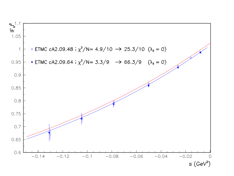
In contrast with the preceeding Subsection (no dealing with the spacelike data), using a second degree and rescaling the spectra, while improving the sector, leads to a degraded account of the spacelike data () and a loss of the remarkable prediction of the LQCD pion form factor data [57] reported in [19]; this is illustrated by Figure 1. Comparing this Figure with Figure 8 of [19], derived by excluding the data from the fit, one observes a good agreement with EBHLS solution1616 16 In the broken HLS frameworks, the pion form factor fulfills ; when is left free, the fit returns a departure from 1 by 2 permil whereas it becomes 1.3 percent when is fixed to zero. This is the origin of the ”shift” exhibited by the two curves shown in Figure 1.. Finally, the last two data columns in Table 2 show that EBHLS2 perfectly succeeds in recovering uniformly good ’s with fit probabilities exceeding 90% and a fair account of all channels.
3.4 Summary
Therefore, once including the data within the BHLS2 minimization procedure, a fit using a third degree succeeds, reminding the conclusions already reached in [19]; however, one has to accept an average of 1.95 for Belle, whereas those for Aleph and Cleo are resp. 0.62 and 1.18.
The fact that A, B and C carry a common lineshape may look hardly accidental. However, in contrast with Table 1, where an evidence for solely a rescaling looks reasonable, Table 2 indicates that a mere rescaling is insufficient – not even mentioning that the EBHLS2 prediction for the LQCD pion form factor data [57] severely degrades compared to [19]. In this case, EBHLS2 – complemented or not with a common rescaling of the spectra – performs nicely and fulfills all desirable Analyticity requirements using a second degree only, as should be preferred. The fits reported in Subsections 3.2 and 3.3 convincingly illustrates that the third degree looks somewhat ad hoc and can be avoided.
Therefore, one is led to complement the Covariant Derivative (CD) breaking introduced in [19] by an additional term (see Section 4) which breaks the kinetic sector of the HLS Lagrangian. This points toward a violation of CVC in the sector (at a level for ). For completeness, one has also examined the effect of a possible rescaling complementing the CVC breaking (generated by a non-zero ); this is reported in the last data column of Table 2. This rescaling may correspond to a (higher order?) correction to the product (at a level). However, this additional freedom does not produce a significant effect and is discarded from now on.

To conclude, the present analysis leads to stress the importance of having at disposal a new high statistics dipion spectrum; it is, indeed, of importance to conclude about the specific behavior exhibited by the Belle spectrum within global fits. The challenging properties exhibited by fitting the dipion spectra or, alternatively, their lineshapes may look amazing enough to call for a confirmation of the Belle spectrum properties. Indeed, it is not unlikely that the much higher statistics of the Belle spectrum (50 times those of Cleo [21]) allows a finer structure to show up, calling for a more refined description.
4 Extending the BHLS2 Breaking Scheme
The Hidden Local Symmetry Model [13] has been supplied with specific symmetry breaking mechanisms to provide the BHLS2 framework [19] within which almost all annihilation channels occuring up to the mass are encompassed. This allowed for a simultaneous fit of almost all collected data samples covering the non–anomalous decay channels (, , ) and anomalous ones [12] (, , ). As clear from [19], one gets a fair description with superb goodness of fit.
As just emphasized in Section 3, the decay mode is also a natural part of the successive HLS frameworks [58, 59, 41, 14, 19]. However, as illustrated by Table 2, the issue is whether, one requires (or not) to consider, besides the ALEPH [22] and Cleo [23] spectra, those from Belle [21]. Our present goal is to define an extension of BHLS2 which can naturally encompass simultaneously the A, C and B spectra and continuously recover the BHLS2 framework in some smooth limit. Anticipatively, this extension has been named EBHLS2.
BHLS2 has been constructed by considering, beside the BKY mechanism [16, 17], the Covariant Derivative Breaking and the Primordial Mixing procedures – see Sections 4 and 8 of [19]. These essentially address the vector sector of the HLS Model and rotations allow to render BHLS2 Lagrangian canonical. This lets also the vector meson kinetic energy supplied by the Yang–Mills Lagrangian be canonical.
Regarding the pseudoscalar (PS) sector, the BKY mechanism [16, 17, 14] also contributes to break the symmetries of the HLS Model. One should also emphasize that the mass breaking in the kaon sector is at the origin of the Dynamical Mixing of the vector mesons [58], which is the central piece of the various broken versions of the HLS model. Indeed, thanks to having different charged and neutral kaon loops, the (, , ) mass matrix at one loop becomes non–diagonal and, thus, imposes another step in the vector field redefinition [14, 19]. This forth and back play between vector field redefinition and Isospin Symmetry breaking in the PS sector should be noted.
Beside the two mechanisms just listed, in order to account for the physics of the anomalous processes, the ’t Hooft determinant terms [20], more precisely its kinetic part, provide the needed nonet symmetry breaking in the PS sector. Moreover, higher order and loop terms in Chiral Perturbation Theory and QED corrections are expected to extend the breaking of the PS kinetic energy term beyond the singlet component. It is the purpose of the present Section to extend the kinetic breaking1717 17 The recent [60] develops such a kinetic breaking focusing on a treatment of the system. Former studies, like [61, 62] for instance, already considered such a breaking mechanism. the full system; one already knows from the preceeding Section that it provides a consistent picture of the sector as it renders consistent the account of the A, C and B spectra.
Once these symmetries have been broken, the PS kinetic energy term of the HLS Lagrangian is no longer diagonal and a field redefinition is mandatory to restore its canonical form1818 18 Regarding the vector meson sector, the layout of the full renormalization procedure has been already defined and thoroughly described in [19]; it applies here without any modification and will not be rediscussed.. This is performed in the two steps addressed right now.
4.1 Diagonalization of the PS Kinetic Energy Piece
In the BHLS/BHLS2 model, the pseudoscalar (PS) kinetic energy term writes [14, 19] :
| (9) |
where is the so–called BKY breaking matrix at work in the sector of the BHLS2 non-anomalous Lagrangian [19] (); combining the new breaking scheme defined in [17] and the extension proposed in [18], it writes [14] :
| (10) |
The departure from unity of the and entries ( and ) of , numerically small [14], are treated as perturbations1919 19 We have already defined heuristically the first non–leading order in perturbative expansions by some generic (perturbation) parameter; this notation is prefered to the previous naming used in our [19] to avoid confusion with breaking parameters to be introduced below. in amplitude calculations whereas occuring as the entry is expected and treated as ; this entry can be also referred to as flavor breaking [37, 35, 36]. Assuming the pion decay constant occuring in the HLS based Lagrangian models is the observed one, its renormalization is unnecessary and has been shown to imply [14] . Therefore, phenomenologically, one is left with only two free parameters, and .
To restore the PS kinetic energy of the piece of the BKY broken HLS Lagrangians to canonical form, a first field transform [31] is performed :
| (11) |
is the (first step) renormalized PS field matrix which brings back into canonical form. One has :
| (12) |
which defines the matrix . We use the notation to remind the specific Gell-Mann matrix to which the neutral pion is associated, and devote the notation to the corresponding mass eigenstate. The entries of in Equation (12) are given by :
| (13) |
which are used all along this study. For further use, Equation (12) is re-expressed :
| (14) |
In terms of the renormalized fields, is thus canonical :
| (15) |
The following expression of in the algebra canonical basis clearly exhibits the precise structure of the BKY breaking procedure :
| (16) |
where is the unit matrix. complements the usual Gell–Mann matrices normalized by Tr.
Displayed in this way, the departure from unity of the breaking matrix exhibits its 3 expected contributions. , a purely Isospin Symmetry breaking (ISB) parameter, is associated with as it should. In contrast, the effect of the flavor breaking amount will be met several times below. Its origin is naturally shared between and ; both simultaneously vanish in the ”no–BKY breaking” limit . So, as expected, the BKY matrix entry, combines correlatedly and Nonet Symmetry (NSB) breakings in the PS sector. Let us also note that [19] as will be reminded below in the EBHLS2 modified context – see Equations (71).
4.2 The Kinetic Breaking : A Generalization of the ’t Hooft Term
A more direct breaking of the symmetric PS field matrix to has also been found phenomenologically requested to succesfully deal with the whole BHLS realm of experimental data [14, 19]. These are the so–called ’t Hooft determinant terms [20, 32, 33, 31]; limiting oneself here to the kinetic energy term, one has been led to supplement the HLS kinetic energy piece by :
| (17) |
where is the usual symmetric pseudoscalar bare field matrix [14, 19] and the (measured) charged pion decay constant. This relation is connected with by the identity :
Expanding in Equation (17), the leading order term is2020 20 In the literature, is named [32, 33, 37]. Removing the derivative symbols in Equation (17) generates a singlet mass term – the topological susceptibility – to account for the mass. :
| (18) |
only involving the singlet PS bare field .
The ’t Hooft term tool, already used in the previous broken HLS versions, can be fruitfully generalized. Indeed, Equation (17) can be interpreted as :
| (19) |
where2121 21 Assuming be positive, which is supported by our former fit results [14, 19]. .
Equation (19) gives a hint that other well-chosen forms of the matrix may exhibit interesting properties. Indeed, it clearly permits to define mechanisms not limited to only nonet symmetry breaking. This leads us to propose the following choice for :
| (20) |
as it manifestly allows for a breaking of Isospin Symmetry and enrich the HLS Model ability to cover the mixing properties. As will be seen shortly, it also leads to differentiate the pion pair couplings to and . With this choice, Equation (19) becomes at leading order :
| (21) |
This form for is certainly not the unique way to generalize the usual ’t Hooft term. For instance, among other possible choices, one could quote :
| (22) |
which turns out to drop the crossed terms in Equation (21) – and in all expressions reported below. On the other hand, as will be seen in Section 16, it happens that a generalization such as Equation (20) is necessary to allow BHLS2 to fulfill expected properties of the axial currents in a non-trivial way.
In order to deal with kaons or charged pions, one could also define appropriate projectors ; however, this does not look necessary as the BKY breaking already produces the needed breaking effects [14, 19].
In the broken HLS frameworks previously defined, the (single) ’t Hooft breaking parameter was counted as when truncating the Lagrangian to its leading order terms in all the previously defined BHLS2 breaking parameters [19]. Consistency, thus, implies to count all the just introduced as .
4.3 The PS Kinetic Energy of the Extended BHLS2 Lagrangian
The full PS kinetic energy term of the broken HLS Lagrangians is provided by their Lagrangian piece :
| (23) |
Performing the change of fields of Equations (12) which diagonalizes and using as given in Equation (20), the full kinetic energy term can be written :
| (24) |
omitting the kaon and (charged) pion terms which are standard and displayed elsewhere [14, 19]. We have defined :
| (25) |
where , , are given by Equations (13). One should note the intricate combination of the ’t Hooft breaking parameters with the BKY parameter .
Defining the (co-)vector , can be written :
| (26) |
being the sum of the unit matrix and of a rank 1 one writes :
| (27) |
The second step renormalized fields are defined by :
| (28) |
which brings the kinetic energy into canonical form :
| (29) |
5 PS Meson Mass Eigenstates : The Physical PS field Basis
The PS field basis renders the kinetic energy term canonical; nevertheless, this basis is not expected to diagonalize the PS mass term into its mass eigenstates (). Indeed, for instance, up to small perturbations, the and are almost pure singlet and octet field combinations, while the physically observed and mass eigenstate fields are mixtures of these. In order to preserve the canonical structure of the PS kinetic energy one should consider the transformation from fields to the physically observed mass eigenstates; as the PS mass term (not shown) is certainly a positive definite quadratic form, this transformation should be a pure rotation.
In the traditional approach, the physical and fields are related to the singlet-octet states by the so–called one angle transform :
| (32) |
However, extending to the mass eigenstate () triplet, one expects a 3–dimensional rotation and thus 3 angles. Adopting the Leutwyler parametrization [39], one has :
| (33) |
to relate the fields which diagonalize the kinetic energy to the physical (i.e. mass eigenstates) neutral PS fields. The three angles occuring there (, and even ) are assumed perturbations; nevertheless, it looks better to stick close to the one–angle picture by keeping the trigonometric functions of , the so–called third mixing angle [31]; for clarity and for the sake of comparison with other works, is not treated as manifestly small. The Leutwyler rotation matrix can be factored out into a product of 2 rotation matrices :
| (34) |
Substantially, the second matrix in the right-hand side of Equation (34) reflects Isospin breaking effects. In the following, one names and the two matrices showing up there; they fulfill :
| (35) |
up to terms of degree higher than 1 in . This implies [39] :
| (36) |
6 Extended BHLS2 : The Non–Anomalous Lagrangian
The non–anomalous EBHLS2 Lagrangian in the present approach can also be written :
| (37) |
as in [19]. As in this Reference, one splits up the first two terms in a more appropriate way :
| (38) |
essentially adresses the physics of the annihilations to charged pions and to kaons pairs; within the present breaking scheme, it remains strictly identical to those displayed in Appendix A.1 of [19]. The is also unchanged as it does not address PS mesons interactions; it is identical to those displayed in Appendix A.3 of [19]. Both pieces have not to be discussed any further and their expressions will not be reproduced here to avoid lengthy repetitions.
All modifications induced by the generalized ’t Hooft kinetic breaking mechanism are concentrated in the piece and are displayed right now. Using2222 22 As stated in Section 2, the breaking parameter is phenomenologically out of reach and one imposes within our fits; it is, nevertheless, kept in the model expressions for information. () :
| (39) |
the expression of in terms of bare PS fields is given, at lowest order in the breaking parameters, by :
| (40) |
where one has limited oneself to only display the terms relevant for our purpose. The (classical) photon and mass terms [13, 17] are not considered and are given only for completeness. However, it is worth reminding that the photon mass term does not prevent the photon pole to reside at as required [63], at leading order. The interaction part of can be split up into several pieces. Discarding couplings of the form , one can write :
| (41) |
with :
| (42) |
and :
| (43) |
where the subscript indicates that the field is bare. Equations (31) provide the relationship between bare and renormalized states, in particular :
| (44) |
The occurence of the parameter generates a decoupling of the and interaction intensities. Using also Equation (36), Equations (43) and (44) give at first non–leading order :
| (45) |
in terms of physical neutral PS fields, and then :
| (46) |
Once more, the rest of the is unchanged compared to their BHLS2 expressions [19].
Regarding the pion form factor in the decay, the changes versus Subsection 11.1 in [19] and the present EBHLS2 are very limited :
| (47) |
This implies a global rescaling of the BHLS2 pion form factor by ; it also implies that the loop acquires a factor of . The BHLS2 transition amplitude and the propagator are changing correspondingly (See Subsection 11.1 in [19]). On the other hand, remains identical to its BHLS2 expression, as well as both kaon form factors.
7 Extended BHLS2 : The Anomalous Lagrangian Pieces
If only the part of the non–anomalous BHLS2 Lagrangian is affected by the kinetic breaking presented above, all the anomalous FKTUY pieces [12, 13] are concerned.
The Lagrangian pieces of relevance for the phenomenology we address are, on the one hand :
| (48) |
where is the usual quark charge matrix and , and denote resp. the electromagnetic field, the vector field matrix and the U(3) symmetric bare pseudoscalar field matrix as defined in [14] regarding their normalization. As one did not find any important improvement by assuming , the difference of these has been set to zero; consequently, the Lagrangian piece [13] drops out.
On the other hand, the following pieces should also be considered :
| (49) |
These involve, beside and , a third parameter which is also not fixed within the HLS framework [13] and should be derived from the minimization procedure. In order to ease the reading of the text we have found it worth pushing them in Appendices A and B.
Regarding the pseudoscalar fields, the Lagrangian pieces listed in Appendices A and B, are expressed in terms of the physically observed whereas, for simplicity, the vector mesons are expressed in terms of their ideal combinations : and . The procedures to derive the couplings to the physically observed and and construct the cross-sections for the annihilations are given in full details in Section 12 of [19]. Nevertheless, one has found worthwhile to construct the amplitude and the cross-section for the annihilations in the Extended BHLS2 framework; this information2323 23 One may note that in Equation (144) corrects for an error in [19] missed in the Erratum (). is provided in Appendix C.
8 Update of the 3 Annihilation Channel
The BESIII Collaboration has recently published the Born cross section spectrum [24] for the annihilation over the GeV energy range collected in the ISR mode. This new data sample comes complementing the spectra collected at the VEPP-2M Collider by CMD2 [64, 43, 65, 66] and SND [67, 68] covering the and peak regions. Besides, the only data on the 3 cross section stretching over the intermediate region was collected much earlier [69] by the former Neutral Dectector (ND). As the measurement by BaBar [70] only covers the GeV region, it is of no concern for physics studies up to the signal. On the other hand, previous independent analyses [71, 19] indicate that the CMD2 spectrum [66] returns an average per point much above 2 units which led to discard it from global approaches.
The BESIII sample [24] is the first 3 pion sample to encompass the whole range of validity of the HLS Model, providing a doubling of the number of candidate data points and, additionally, the first cross-check of the cross section behavior in the energy region in between the narrow and signals.
We first examine how it fits within the global HLS framework in isolation (i.e. as single representative of the 3 annihilation channel) and conclude about its consistency with the already analyzed data samples covering the other annihilation channels, namely , and both modes. A second step is devoted to consistency studies between the BESIII spectrum and those previously collected in the same 3 channel by the ND [69], CMD2 [64, 43, 65] and SND [67, 68] detectors.
8.1 The BESIII 3 Data Sample in Isolation within EBHLS2
The fit procedure already developped within the previous BHLS frameworks [14, 19] – and closely followed here – relies on a global minimization. In order to include the BESIII sample within the EBHLS2 framework2424 24 Actually, the 3 channel is marginally sensitive to the differences between BHLS2 and its extension to EBHLS2., one should first define its contribution to the global . This requires to define the error covariance matrix merging appropriately the statistical and systematic uncertainties provided by the BESIII Collaboration together with its spectrum and paying special care to the normalization uncertainty treatment. This should be done by closely following the information provided together with its spectrum by the Collaboration2525 25 In the process of sample combination frameworks, additional issues may arise; for instance, the consistency of the absolute energy calibration of the various experiments with each other should be addressed as done in [19] with the dikaon data samples collected by CMD3 [72, 73] and BaBar [40]..
For definiteness, the data point of the BESIII sample [24] at the energy squared is :
using obvious notations; it is useful to define , the experimental fractional systematic error. Then, the elements of the full covariance matrix associated with the BESIII spectrum write :
| (50) |
where the indices run over the number of data points (). is the (diagonal) matrix of the squared statistical errors (), and is the reported fractional systematic error at the data point of energy (squared) , defined as just above. The systematic errors are considered point-to-point correlated and reflecting a (global) normalization uncertainty.
At start of the fit iterative procedure, the natural choice for is the vector of measurements itself (); in the iterations afterwards, it is highly recommended [74, 75, 76] to replace the measurements by the fitting model function () derived at the previous iteration step for the concern of avoiding the occurence of biases. Then, the experiment contribution to the global writes :
| (51) |
Moreover, a normalization correction naturally follows from the global scale uncertainty. It is a derived quantity of the minimization procedure. Defining the vector (), this correction is given by [76, 19] :
| (52) |
For the purpose of graphical representation, one could either perform the replacement , or apply the correction to the model function . When comparing graphically several spectra, the former option should clearly be prefered as, indeed, even if not submitted to the fit, other parent data samples can be fruitfully represented in the same plot by performing the change2626 26 Numerically, is derived by using the function values at the central values of the fit parameters. :
using the BESIII fit function . Such a plot is obviously a relevant visual piece of information.
A global fit involving all data covering the , and both channels and only the BESIII spectrum to cover the 3 annihilation final state has been performed and returns, for the BESIII sample2727 27 We have prefered skipping the first few data points more subject to non–negligible background; the spectrum is thus fitted in the energy range GeV. , .
The top panels in Figure 3 display the distribution of the BESIII normalized residuals corrected as reminded just above. In the region, at least, the normalized residual distribution is clearly energy dependent. The normalized (pseudo-)residuals of the unfitted data samples displayed2828 28 For short, these will be referred to below as NSK., namely those from [42, 67] in the region and from [64, 68] in the region, likewise corrected for the normalization uncertainty, are, instead, satisfactory2929 29 Thus, the normalization correction applied to each of the NSK 3 data samples is determined by the fit of solely the BESIII data [24] within the global framework., despite being unfitted. The fit process allows to compute the (global) distance of the NSK samples to the (BESIII) fit function and returns , a reasonable value for unfitted data.
However, the behavior of the BESIII residuals may indicate a mismatch between the and pole positions in the BESIII sample compared to the other () data samples involved in the (global) fit; indeed, the narrow and signals are already present in the and channels, and therefore, as when dealing with the CMD3 and BaBar dikaon samples in [19], a mass recalibration (shift) could be necessary to avoid mismatches with the pole positions for and in the other data samples. We thus have refitted the BESIII data, by allowing for such a mass shift to recalibrate the BESIII energies and match our reference energy scale3030 30 Our reference energy is actually defined consistently by more than 50 data samples. As an important part of these has been collected at the VEPP-2M Collider in Novosibirsk, we denote, when needed, our reference energy by .. So, we define :
and let vary within the fit procedure. The fit returns keV with and, thus, the (noticeable) gain of 29 units should be attributed to only allowing for a non-zero . The corresponding normalized residuals, displayed in the middle row of Figure 3, are clearly much improved, whereas the distance of the NSK 3 data sample to the BESIII fit function stays alike.

Owing to the sharp improvement produced by this mass shift, it was tempting to check whether the energy (re-)calibration could be somewhat different at the and the masses. For this purpose, it is appropriate to redefine the fitting algorithm by stating ;
| (53) |
where should be chosen appropriately, i.e. significantly outside the and peak energy intervals. As obvious from the bottom panel of Figure 5, the 3 cross section in the intermediate energy region is almost flat and indicates that the choice for is far from critical; one chose GeV.
The corresponding global fit has been performed and returns , an additional gain of 18 units comes, to be cumulated with the previous 29 unit gain. The recalibration constants versus are :
After having applied this recalibration, the BESIII normalized residuals, shown in the panels of the bottom row in Figure 3, are observed flat, as well as their NSK partners also displayed.
One should remark that is in striking correspondance with the central value for the energy shift reported by BESIII [24] compared to their Monte Carlo ( MeV) and is found highly significant (about ). is also consistent with this number but quite significantly different from . Actually, comparing the three rightmost panels in Figure 3, one observes that the main gain of decorrelating the energy calibration at the and peaks widely improves the former energy region; the later looks almost insensitive, as reflected by the fact that the non-zero is only a effect.
So, once two energy recalibrations have been performed, the description of the BESIII sample is quite satisfactory and, fitted with the other annihilation channels, the probability is comfortable (91.6%).
At first sight, the differing energy shifts just reported may look surprising as, for ISR spectra, the energy calibration is very precisely fixed by the energy at which the accelerator is running at meson factories. However, such energy shifts could be related with unaccounted effects of the secondary photon emission expected to affect the resonances showing up at lower energies. In the case of the BESIII spectrum, this concerns the and regions, where photon radiation effects get enhanced by the resonances, causing shifts between the physical resonance parameters and their observed partners3131 31 Note that, for the NSK scan experiments, photon emission on resonances is corrected locally resonance by resonance. . This topic is specifically addressed in Appendix D, where it is shown – and illustrated by Table 14 therein – that the expected shifts produced by secondary ISR photons are in striking correspondence with the fitted and .
8.2 Exploratory EBHLS2 global Fits including the BESIII 3 Sample
Having proved that the BESIII 3 data sample suitably fits the global EBHLS2 framework, we perform the analysis by merging the BESIII and the parent CMD2 and SND data samples within a common fit procedure. For completeness, we have first performed a global fit allowing for a single energy calibration constant. The fit returns and 84.7 % probability. The values for BESIII (154/128) and NSK (145/158) are also reasonable, however, the normalized residuals for BESIII shown in the top panels of Figure 4 – especially the leftmost panel – still exhibit a structured behavior.

Therefore we have allowed for two independent energy shifts and within the iterative fit procedure. Convergence is reached with and 91.2% probability. The values for BESIII (137/128) is improved by 17 units whereas it is unchanged for NSK (147/158); so, the improvement of the total only proceeds from the 17 unit reduction of the BESIII partial . The bottom panels in Figure 4 are indeed observed flat in the and regions (this last distribution is still less sensitive to the fit quality improvement). The energy recalibration constants of the BESIII data with regard to the NSK energy scale are :
in fair accord with those derived in the global fit performed discarding the NSK 3 data. Compared to its fit in isolation, the BESIII data is degraded by 137-123=14 units, while (see Table 4 third data column) the NSK data is degraded by 147-135=12 units compared to the fit performed discarding the BESIII data sample, the rest being unchanged. Regarding the average per data point, the degradation is of the order 0.1 –unit for both the NSK and BESIII samples, a quite insignificant change. So, one can conclude that the full set of consistent data samples can welcome the BESIII sample [24], once the energy shifts and are applied.
Figure 5 displays the fit function and data in the 3 channel. All data are normalization corrected as emphasized above and, additionally, the energy shifts induced by having different and calibration constants are applied to the BESIII data sample; one should also note the nice matching of the ND and BESIII data in the intermediate region. Additional fit details of this new global fit are given in the third data column of Table 4.

9 Revisiting the Annihilation Channel
A fair understanding of the dipion annihilation channel, which provides by far the largest contribution () to the muon HVP, is an important issue. Fortunately, the cross-section is also the most important channel encompassed within the BHLS [14, 76] and BHLS2 [19] frameworks previously developped. All the existing dipion data samples were examined within the context of these two variants of the HLS Model. As some of them exhibit strong tensions [14] with significant consequences on the derived physics quantities, it looks worthwhile to revisit this issue when a new measurement arises, at least to check if the consistency pattern previously favored deserves reexamination.
Beside the data samples formerly collected and gathered in [77], an important place should be devoted to the data from CMD-2 [78, 43, 44] and SND [45] collected in scan mode on the VEPP-2M collider at Novosibirsk; these CMD2 and SND samples are collectively referred to below as NSK. These were followed by higher statistics samples, namely, the KLOE08 spectrum [28] collected at Dane and those collected by BaBar [79] at PEP-II, both using the Initial State Radiation (ISR) method [80]. Slightly later, the KLOE Collaboration produced two more ISR data samples, KLOE10 [46] and KLOE12 [47], the latter being tightly related with KLOE08 (see Figure 1 in [81]). In this reference, the KLOE-2 Collaboration has also published a dipion spectrum derived by combining the KLOE08, KLOE10 and KLOE12 spectra; this combined spectrum is referred to below as KLOE85, thus named according to its number of data points.
Two more data samples, also collected in the ISR mode, were appended to this list by BESIII [26] – with recently improved statistical errors [27] – and a CLEO-c group [48]. Finally, the SND collaboration has just published a data sample [25] collected in scan mode on the new VEPP-2000 Facility at Novosibirsk; this spectrum, seemingly still preliminary, is referred to below as SND20. Another high statistics data sample, also collected in scan mode, is expected from the CMD3 Collaboration [82].
Important tension between some of these samples – namely KLOE08 and BaBar – and all others have already been identified [76, 2]; the occurence of the new data sample from SND (and its comparison with NSK, KLOE and BaBar [25]) allows to reexamine this consistency issue and gives the opportunity to remind how it is dealt within global frameworks.
9.1 The Sample Analysis Method : A Brief Reminder
The broken HLS modelings previously developped, especially BHLS2 as well as its present extension, aim at providing frameworks which encompass a large part of the low energy physics, the realm of the non-perturbative regime of QCD, and extend up to the mass region; they have rendered possible fair simultaneous accounts of the six major annihilation channels (, , , , ) up to 1.05 GeV/c; slightly modified (EBHLS2), this framework also provides now a satisfactory understanding of the A, B and C dipion spectra from the decay of the lepton.
As already noted several times, the Lagrangians which substantiate the various broken HLS models emphasize a property expected from QCD : The different annihilation channels should be correlated via their common underlying QCD background; this is reflected within our Effective Lagrangians by the fact that all their model parameters are simultaneously involved in the amplitudes for any of the accessible physics processes they encompass. A straightforward example is represented by , the universal vector coupling and this property is, more generally, exhibited by the expressions for the various amplitudes derived from within the various broken HLS Lagrangians.
Most of the Lagrangian parameters are not known ab initio and are derived from the data via a global fit involving all channels and, possibly, all available data samples. For this purpose, the provided data samples and associated information (data points, statistical errors, systematics, correlated or not) are supposed reasonably3232 32 Of course, it is unrealistic to expect that the spectrum and uncertainties defining any data sample have been perfectly determined- see below. well estimated. With this at hand, one can construct a motivated global and derive the Lagrangian parameters through a minimization procedure like minuit.
Among the various kinds of uncertainties reported by the different experiments, a special care should be devoted to the global normalization uncertainties – which can be energy dependent as already dealt with in Subsection 8.1. Actually, as for energy scale recalibrations (see also Subsection 8.1), it looks obvious that the most appropriate normalization of a given sample can only be determined by comparing with several other independent spectra covering the same physics channel. Even more, a global treatment of these provides the best normalization of each sample versus all the others by a kind of bootstrap mechanism.
Actually a global fit, when possible, looks the best tool to determine the most appropriate normalization of each spectrum in accord with its reported uncertainties, including its normalization uncertainties; this is reminded in details in [76, 19] and above in Section 8. The goodness of the corresponding fit tells the confidence one can devote to the normalization corrections.
The probability of the best fit reflects the quality of the experimental information and the relative consistency of the various data samples involved in the procedure within the model framework; we have now 3 significantly different HLS frameworks at hand which have been shown in [19] and just above to lead to a consistent picture.
9.2 Samples Covering the Channel : A Few Properties
Let us first consider the data samples already identified as not exhibiting significant tension among them within the BHLS2 frameworks, the previous one [19] or the present one; this defines a Reference set of data samples, named . This already covers the data samples already considered in Section 8 and all the existing data samples covering the and decay channels. Regarding the dikaon spectra, we refer the reader to our analysis in [19] where the tensions between the CMD3 spectra [73, 72] and the others from SND, BaBar and (corrected [19]) CMD2 has led to discard them from the analysis3333 33 The CMD3 data have, nevertheless, been dealt with to estimate systematics in the muon HVP evaluation [19]. . As for dipion spectra, it has been shown in Section 4 that the residual tension observed in the account for Belle compared to Aleph and Cleo can be absorbed. The reference set also includes the spacelike pion [55, 56] and kaon form factor spectra [83, 84] which are satisfactorily understood within the BHLS2 frameworks [19].
For the purpose of reexaming sample tensions, it looks appropriate to also include in , the pion form factor spectra collected by BESIII [26, 27] and Cleo-c [48]. Indeed, anticipating somewhat on our fit results, it has been observed that, alone or together with either of the NSK, KLOE, BaBar samples, or with any combination of these, they get the same individual sample ’s, with fluctuations not exceeding 1.5 units for each of them. Fitting the sample set thus defined within the present framework returns and a 94% probability; in this fit, the BESIII and Cleo-c samples yield
One can consider the probability of the global fit (here 94%) as a faithful tag of mutual consistency of the (more than 50) samples included in which fairly fit the broken HLS framework.
| [Prob] | + NSK | + KLOE | + BaBar |
|---|---|---|---|
| NSK (127) | [95.3%] | [91.2%] | [51.7%] |
| KLOE (135) | [91.2%] | [95.2%] | [31.9%] |
| BaBar (270) | [51.7%] | [31.9%] | [62.9%] |
We have made two kinds of global fits :
- •
i) Fits involving and each of NSK, KLOE3434 34 KLOE indicates the simultaneous use of KLOE10 and KLOE12 and BaBar in turn; the diagonal in Table 3 reports the main results, namely the value returned for of resp. NSK, KLOE, BaBar and the probability of the global fit at the corresponding Table entry.
- •
ii) Fits involving and the pairwise combinations (NSK, KLOE), (NSK, BaBar) and (KLOE, BaBar) in turn; the main fit results are reported in the non-diagonal entries of Table 3. In order to make easier the comparison of each of the NSK, KLOE, BaBar accounts provided by these ”pairwise” fits, we have organized the non-diagonal entries in a specific manner : The entry (NSK, KLOE) provides and the global fit probability whereas the entry (KLOE, NSK) provides and the (same) fit probability. The same rule applies mutatis mutandis to the other pairwise fits : (NSK, BaBar) and (KLOE, BaBar) together with .
Relying on Table 3, one clearly observes that the single mode fits for NSK and KLOE are fairly good and in nice accord with the results returned by the corresponding pairwise fit. The pattern is somewhat different when BaBar is involved.
In order to be complete, let us briefly summarize the fit results obtained within the present framework concerning KLOE08 and the KLOE85 sample derived by the KLOE2 Collaboration from their combination of the KLOE08, KLOE10 and KLOE12 spectra[81].
- •
Regarding KLOE08 : The global fit for + KLOE08 returns and a 74.7% global fit probability. With an average , one does not consider confidently the results derived from fit to this combination compared to KLOE10+KLOE12.
- •
Regarding KLOE85 : The fit for + KLOE85 returns (global fit probability 94.7%) which clearly indicates that the KLOE08 issue is reasonably well dealt within the KLOE85 combination [81].
One has also performed the pairwise fit + KLOE85 + NSK. In this case, one gets :
with a 80.7% probability. This fit is obviously reasonable3535 35 One should note that the estimates for marginally differ : ( + NSK + KLOE) and ( + NSK + KLOE85) in units of . but less satisfactory than + NSK + KLOE, as the tension between KLOE85 and NSK is large, much larger than when using +NSK + KLOE as displayed in Table 3.
9.3 The case for the 2020 SND Dipion Sample : Fits in Isolation
In order to analyze the new data sample recently provided by the SND Collaboration [25], the treatment of the reported systematic errors has been performed as emphasized above for the data from BESIII (see Subsection 8.1) as the systematics are expected to be fully point-to-point correlated3636 36 There is no explicit statement in [25] about how the systematics should be understood; however, this assumption corresponds to what is usually understood with the data collected at the Novosibirsk facilities. This topic is further discussed just below. . For the present analysis, we have first performed global fits3737 37 For convenience, here, the annihilation channel and data are discarded from the fit procedure. where the single representative for the annihilation channel is SND20, the new SND data sample [25]; the spacelike pion form factor data [55, 56] have also been discarded from the fits in isolation. Figure 6 summarizes our results.
The top panel in Figure 6 indicates that, in single mode, the best fit returns a reasonable probability. However, this comes together with a large average (to be compared with the diagonal in Table 3). Nevertheless, amazingly, the SND20 form factor derived from this global fit provides a fairly good account of the NSK (CMD2 and SND) data not submitted to the fit as one yields , much better than SND20 itself. The NSK (pseudo-)residual spectrum is consistent with flatness and, addtionally, the ratio indicates that there no significant energy calibration mismatch between the NSK samples and SND20 – this may have shown up in the drop-off region.
The bottom panel in Figure 6 displays results derived by assuming the SND20 systematics fully uncorrelated (i.e. the non-diagonal elements of the error covariance matrix are dropped out). The global fit is successful and returns a 92% probabability. The gain for SND20 is noticeable as and, clearly, the (alternative) pion form factor derived by fitting only the SND20 data (in this manner) within the global framework is almost unchanged; this is the way the distance of the NSK samples to this alternative fit form factor can be understood : . Moreover, once again, the NSK (pseudo)residual distributions are as flat as (and almost identical to) those displayed in the top panel of Figure 6.

We got substantially the same results and conclusions by enlarging the SND20 pion form factor statistical errors3838 38 The pion form factor squared Table in [25] gives numbers with only one decimal digit, so adding 0.04 to the statistical uncertainty rounds down to 0. by 0.04 and keeping unchanged the systematics – i.e. treated as point-to-point correlated; this also points towards the interest to have, beside information on correlations, information on the accuracy of the uncertainties [2]. So, the way the SND20 uncertainties should be understood deserves clarification.

9.4 The case for the 2020 SND Dipion Sample : Pairwise Fits
An interesting topic addressed in [25] is the consistency of SND20 with respectively NSK (e.g. CMD2 [78, 43, 44] and SND-98 [45]), KLOE ( KLOE10 [46] and KLOE12 [47]) and BaBar [79]. For this purpose, it looks worthwhile performing global fits by including pairwise combination to cover the annihilation channel3939 39 It has been found appropriate to re-introduce the spacelike data from [55, 56] within the minimization procedure. As the pion form factor in the spacelike and timelike regions is the same analytic function, this is a constraint.. This allows to observe the tension between the partners in the pair and to get a probability which emphasizes their global consistency. Our main fit results are collected in Figure 7.
The middle panel in Figure 7 shows the case for the global fit with the (SND20+NSK) combination. As could be expected, this confirms the fit of SND20 in isolation reported in the top panel of Figure 6 : is negligibly improved whereas is unchanged; the large value for is responsible for the global fit probability reduction compared to fits with NSK alone (or combined with KLOE), as can be seen in Table 3. With this proviso, BHLS2 confirms the statement that SND20 and NSK are consistent [25] with a 73% probability.


In order to address the consistency topic about SND20 and BaBar already studied in [25], we have run our global fit procedure with the (SND20+BaBar) combination. To stick the closest possible to the study reported in [25], we have found it worth to exclude from the fit the part of the BaBar spectrum with . The results are displayed in the top panel of Figure 7 and show some resemblance between SND20 and BaBar (normalized) residuals outside the BaBar excluded region (delimited by the green rectangle). Nevertheless, the fit probability is poor and its indicates a significant tension compared to the fit in isolation ()
Finally, the bottom panel in Figure 7, reports the main fit results obtained by fitting the (SND20+KLOE) combination. One can note the results compared to the fits in isolation : (versus ) while (versus ) and a 37% probability. Here also, one can observe that the residual distributions for SND20 are not really at variance with those for KLOE along the whole energy range.
So, on the whole, the SND20 spectrum [25] does not help in clarifying the consistency issue raised by the existing dipion spectra and, presently, SND20 does not bring in more support, or less support, to the choice performed following our previous analyses (see Tables 4 and 3) and illustrated by Figure 8.
10 Overview of the EBHLS2 Fits
| EBHLS2 | BS () | () | ||
| Excl. | Incl. | BS | RS | |
| NSK (127) | 136 | 134 | 138 | 136 |
| KLOE (135) | 141 | 146 | 139 | 139 |
| BESIII (60) | 48 | 47 | 49 | 48 |
| Spacelike (59) | 62 | 67 | 62 | 60 |
| (ABC) (84) | 93 | 82 | 80 | |
| (112) | 89 | 88 | 88 | 87 |
| (182) | 120 | 120 | 124 | 124 |
| NSK (158) | 142 | 146 | 147 | 147 |
| BESIII (128) | 138 | 138 | 137 | 137 |
| NSK (92) | 103 | 104 | 103 | 104 |
| NSK (49) | 41 | 42 | 39 | 39 |
| BaBar (27) | 41 | 42 | 41 | 41 |
| Spacelike (25) | 18 | 19 | 17 | 18 |
| Decays (8) | 5 | 4 | 9 | 9 |
| 1269/1365 | 1262/1365 | |||
| Probability | 93.3% | 83.1 % | 90.0 % | 91.5 % |
Some of the general properties of the global fits performed in the EBHLS2 framework have already been emphasized in Sections 3, 8 and 9 with special emphasis on resp. the decay dipion spectra, the annihilation channel and the crucial one. The general features of our fitting algorithm concept are detailed in Section 15 of our [19], for instance. Let us, for convenience, remind the gross features of our global fit method :
- •
The contribution of each data sample to the global to be minimized is constructed using solely the uncertainties exactly as they are provided by each experiment without any external input. Additionally, this kind of input may influence the numerical outcome of the fits in an uncontrolled way. On the other hand, if not already performed by the relevant experiments, the reported uncorrelated systematics are merged appropriately with the statistical error covariance matrix,
- •
The correlated systematic errors – possibly -dependent – are treated with special care [76] as emphasized in Subsection 8.1 in order to avoid the so-called Peelle Pertinent Puzzle [85] which generally results in biasing the evaluation of physics quantities based on minimization procedures [86, 87]. Moreover, an iterative procedure is used which has been proved to avoid biases [76].
In the case of a global minimization, it should be stressed that the absolute scale of each experiment is derived in full consistency with those of all the other experiments (or data samples), especially -- but not only -- with those collected by other groups in the same physics channel4040 40 Actually, this looks the natural way, if not the single one, to derive reliably and consistently the correction to the normalization of the various spectra.. Several examples can be found in [19] where it is shown that the derived scale corrections quite well compare with the corresponding experimental expectations.
- •
When merging the different data samples which cover the same energy range, their different energy calibrations may exhibit some mismatch; this issue was previously encountered in our [19] with the energy calibration of the dikaon spectra from CMD-3 [72, 73] and BaBar [40] versus those of the corresponding samples from CMD2 and SND; this issue happened again herein when dealing with the BESIII 3 sample [24] and is solved accordingly (see Section 8 above). It should be noted that, for signals as narrow as the and mesons, global fit technics are certainly the best suited way to match the energy scales of various spectra otherwise poorly consistent.
- •
In order to confidently rely on global fit outputs to evaluate physics quantities, one should discard data samples which exhibit noticeable inconsistencies with the rest of the benchmark samples. Our requirement to identify such samples has generally been to get an average per point smaller than .
Compared to the fits reported in [19] and as already noted in Section 2, we have here released the constraint (Equation(2)) on the product and also let the mixing angle float freely. Moreover, as several preliminary fits typically return :
| (54) |
imposing looks worthwhile; indeed, Equations (54) clearly shows that the physics presently addressed in the EBHLS2 framework does not exhibit a significant sensitivity to these parameters when left free. These constraints will be reexamined4141 41 See below the Sections devoted to the mixing. in the context where the mixing is also addressed.
Table 4 reports the fit results under 4 configurations; the energy scale corrections for the BaBar dikaons [40] and the BESIII samples [24] are floating parameters. The first 2 data columns, actually, update the BHLS2 fit results derived for the BS variant given in [19]; for the fit performed including the spectra, the polynomial here is third degree.
For the EBHLS2 fits reported in the last two data columns, is second degree4242 42 This means that BHLS2 and EBHLS2 actually carry an identical parameter freedom.. The third data column displays the contributions of various groups oyf data samples to the global using the BS configuration. For completeness, the last data column reports the EBHLS2 fit results obtained under its RS configuration [19].
One should note that, substantially, these pure EBHLS2 fits and the BHLS2 fit excluding the spectra (first data column) exhibit similar and favorable averages per point for all groups of data samples with the sole exception of the individual decay modes which is doubled. In the EBHLS2 BS or RS configurations, the single mode which significantly departs from , is , which returns 4, e.g. a difference with the Review of Particle Properties [50]. On the other hand, one may consider, in view of Table 4, that the BS variant of EBHLS2 does not need to be improved by the Primordial Mixing mechanism introduced in [19] to construct the RS variant of BHLS2.
The numerical values of the model parameters of the EBHLS2/BHLS2 framework will be examined and commented in a wider context involving also the treatment of the mixing properties in Section 18.
11 Evaluation of , the Muon HVP
As the previous BHLS releases [14, 19], EBHLS2 encompasses the bulk of the low energy annihilations up to, and including, the mass region. Therefore, taking into account suitably the various kinds of uncertainties reported by the different experiments affecting the spectra they collected, a fully global fit is expected to lead to precise evaluations of the contributions to from the energy region GeV. Within this approach, the specific contribution of the hadronic channel is obtained by means of the cross section with parameter values derived from the global fit performed within the EBHLS2 framework :
| (55) |
[88, 89] is the usual kernel which enhances the weight of the threshold regions compared to the higher energy regions of the spectrum; is the threshold of the hadronic channel and GeV is the validity limit, common to the different HLS frameworks.
11.1 Remarks on the GeV Contribution to
We find it of special concern to substantiate what supports the choices performed in our global fit approach in connection with the muon HVP outcome. For this purpose, the analysis of the channel properties within the (E)BHLS2 framework is of special relevance. Global fits have been performed involving the data samples collected for all the HLS final states except for and complemented in turn by each of the various KLOE samples already commented in [19] to feed solely the channel.
| Data Sample | Direct integration [90] | BHLS2 | (Prob.) |
|---|---|---|---|
| KLOE10 | 69/75 (78%) | ||
| KLOE12 | 59/60 (80%) | ||
| KLOE85 | 95/85 (65%) | ||
| KLOE08 | 130/60 (14%) |
Table 5 – reprinted from Table 3 in [2] – clearly shows that the (E)BHLS2 central values are obviously in close correspondence with those derived by directly integrating the data [90], except for KLOE08 which, correlatedly, exhibits a poor global fit probability; this substantiates the reason why one may prefer discarding poorly fitted data samples to avoid biases, possibly large. However, one should also remark that its effect within the KLOE85 combination is much softer as the KLOE85 fit probability (65%) remains comparable to those for KLOE10 and KLOE12 which are both higher and almost identical (78% and 80 %).
Table 5 also shows the important reduction of the uncertainties induced by the non– channels involved in the reported global fits; this reduction is, of course, amplified when including the other accepted samples in the fit procedure as will be seen shortly. On the other hand, when the fit probability is poor, the values returned by the fits for the uncertainty and the central value should be handled with care.
Table 6 shows a breakdown of the contributions to from different energy intervals. The top lines display the results derived by other groups, namely CHS [91], DHMZ [92] and KNT [93] while the bottom lines show the EBHLS2 outcome from fits performed under the various indicated configurations. The favored configuration, which corresponds to a good account of all the channels encompassed within the EBHLS2 framework, is tagged by ”KLOE+X”. Nevertheless, in order to really compare the global fit method with [91, 92, 93] it is worth relying on the same set of experimental data. To this end, we have also run our code including the BaBar data sample within the set of fitted spectra so that the sample contents are similar in all the discussed approaches; nevertheless, in order to avoid the effects of energy calibration mismatch between the BaBar and KLOE spectra within the fit procedure, we have removed the BaBar drop-off region from the fit. The corresponding results are given in Table 6 under the tag ”KLOE+BaBar+X”.
| Interval (GeV) | ||||
|---|---|---|---|---|
| CHS18 [91] | ||||
| DHMZ19 [92] | ||||
| KNT19 [93] | ||||
| KLOE+BaBar +X | : BaBar=1.45, KLOE=1.15, NSK=1.10 | |||
| Prob=11.4% | ||||
| KLOE +X | : KLOE=1.03, NSK=1.09 | |||
| Prob=90.0% (Incl. ) | ||||
| Prob=93.3% (Excl. ) | ||||
Regarding the reported central values for , it is clear that CHS18, DHMZ19, KNT19 and the evaluation derived from the KLOE+BaBar+X fit are similar; nevertheless, one should point out the higher similarity of the KNT19 and EBHLS2(KLOE+BaBar+X) evaluations. Indeed, the difference between their central values are resp. 0.1, 0.7 and 0.2 for resp. the GeV, GeV GeV and GeV GeV energy intervals. One may infer that this fair agreement is mostly due to having similar treatments of the correlated systematics in the BHLS approaches [76] and in the KNT dealing [93].
As in global approaches the data collected in the non– channels are equivalent to having at disposal an additional statistics in the channel, one expects smaller errors for the (E)BHLS2 evaluations of ; this is indeed what is observed for the GeV and GeV GeV contributions to but, surprisingly, not for the GeV GeV interval. Nevertheless, integrated up to 1.0 GeV, the contribution to exhibits an uncertainty improved by a factor of compared to the other approaches reported in Table 6.
This comparison proves that the observed central value differences between BHLS2 and the others – especially KNT – are mostly due to having discarded BaBar (and KLOE08) and only marginally to the global fit method. Finally, the last 2 lines of Table 6 shows the effect of including the data. The use of these generates an additional (modest) improvement of the uncertainties as could be expected, and a marginal shift. The comfortable probabilities reached by the EBHLS2(KLOE+X) fits should also be noted. As reminded in Section 10, they are reached without resorting to error information beyond what is provided by the various experiments like error inflation factors, for instance.
As noted several times, the validity range of the HLS approaches to annihilations extends up to GeV, thus including the mass region. However, the GeV energy interval of the dipion spectrum is poorly known; indeed, apart from the BaBar spectrum4343 43 Our [15] provided a study of mass region in the BaBar spectrum. [29], the most recent information about this spectrum piece follows from the old SND results [94] which underly the RPP [50] entries for the decay.
As clear from Figure 8, in this mass region the spectrum is widely dominated by the tail of the resonance with, on top of it, a tiny effect due to the narrow signal. A direct numerical estimate derived from the scarce data collected around the mass gives . On the other hand, relying on the RPP [50] information, EBHLS2 returns :
replacing within the data set fitted via EBHLS2 the RPP datum by the BaBar [1.0,1.05] GeV spectrum piece returns . Therefore, some (mild) systematics affects this mass region as the cross section lineshape is not really well defined (see Figure 1 in [15]).
11.2 Contribution to the Muon HVP of the Energy Region GeV
The sum of the quantities defined by Equation (55) represents about 83% of the total muon HVP; it can be computed with fair precision using the EBHLS2 fit information to construct the relevant cross sections; these are derived by sampling the model parameters using the parameter central values and the error covariance matrix returned by the minuit minimization procedure. Sampling out the model parameters allows to compute a large number of estimates for the different and for , the average values of which defining our reconstructed central values and their r.m.s. giving their standard deviations.
The fitted cross sections are also used to estimate the FSR contributions for the , and final states and the Coulomb interaction effect which is significant for the final state as the kaons are slow in the energy region.
The HLS model functions are describing VP amputated data, accordingly, all the data submitted to our global fits are amputated from their photon VP factor. Uncertainties related to VP amputation and FSR estimates are included below as separate systematics.
| EBHLS2 | BS () | () | Data Direct | ||
| Excl. | Incl. | BS | RS | Integration | |
| HLS Sum | |||||
| 1179/1280 | 1285/1365 | 1269/1365 | 1262/1365 | ||
| Probability | 93.3% | 83.1 % | 90.0 % | 91.5 % | |
Regarding the FSR correction of the channel, we assume that the FSR correction of the 2 channel applies to the 2 subsystem of the 3 final state as well. Thus we take as an estimate, assuming that the invariant mass square of the charged subsystem may be approximately identified as . This is justified because the main contribution comes from the enhanced intermediate state , i.e. the resonance enhancement happens at about the same in both the and the channels (see also [95]). One then obtains a FSR contribution to which a 5% error is assigned. The same approximation is accepted by the BESIII Collaboration and their recent 3 spectrum [24] already includes the FSR correction computed this way.
Table 7 collects the results derived from EBHLS2 fits performed under various conditions. The largest difference beween the central values for the HLS sums does not exceed and reflects the effect of using or not the dipion spectra – together with slightly improved uncertainties ( 10%) in the former option. The second data column collects the results derived by assuming and third degree (i.e. the previous BHLS2 framework); the third data column information is derived by letting free and fixing the degree to 2. Despite their different probabilities, their HVP’s differ by only and their uncertainties too. Comparing the third and fourth data columns also shows that the gain achieved by using the Primordial Mixing Mechanism [19] is, by now, negligible.
Therefore, it looks consistent to choose as final evaluation of the BHLS channel contribution to up to GeV :
up to additional systematics considered just below.
On the other hand, the last data column in Table 7 displays the results derived by a direct integration of the annihilation data; in this approach, the normalization of each of the combined spectra is the nominal one and all uncertainties (correlated or not) are combined to provide its weight in the combined spectrum. This brings us back to the discussion presented in the previous Subsection : It is not surprising to observe the data shifting compared to expectations and their uncertainties enlarged by the correlated contributions. This effect is the largest for the contribution but represents only a effect. The difference for the dikaon contributions is rather due to taking the CMD3 data into account in the direct integration whereas they are absent from the set of data samples submitted to the EBHLS2 fit procedure (see [19]); their effect is, nevertheless, taken into account as systematics.
11.3 Systematics in the HLS Contribution of the Muon HVP
Subsection 11.1 has illustrated, specifically on the channel, that a possible hint for a significant bias induced by the global fit method itself is tiny. Indeed, Table 5 shows that, as long as the fit probabilities are good, the values for derived from the fit are very close to the KLOE Collaboration own evaluations [90]. More precisely, the EBHLS2 fit estimates are distant by only resp. , and from the KLOE own direct integration evaluations for resp. KLOE10 (78% prob.), KLOE12 (80% prob.) and the KLOE85 combined data set (65% prob.) The example of KLOE08 is, however, also interesting : Indeed, even if the fit probability is poor (14%) – and for this reason excluded from our reference set of data samples – the fit is away from the KLOE direct integration of this spectrum by only .
On the other hand, the set of accepted data samples being similar, Table 6 also indicates that the way the normalization uncertainty is dealt with accounts for the bulk of the differences between the various approaches. The (similar) choices made by KNT [93] and us [76] look the best grounded one and leads to consistent central values. The better precision reached within the broken HLS frameworks mostly proceeds from the global fit tool they allow which numerically correlates the various annihilation channels as if the statistics in each channel was larger than nominal. One should also remind the marvellous agreement (still valid) between the BHLS2 prediction and the Lattice QCD form factor spectra [57] emphasized in [19] (see Figure 8 therein) – and in Figure 1 above.
Therefore, once a canonical treatment of the various kinds of systematic uncertainties reported by the various groups together with their spectra is applied, one may consider that these are already absorbed in the uncertainties derived from the minuit minimization procedure.
However, additional sources of uncertainty can be invoked. Until EBHLS2 is experimentally strengthened by new high statistics dipion spectra to be collected in the decay, one may consider that the difference between using or not the data contributes a systematic uncertainty which can increase by at most (see Table 7). On the other hand, it is worthwhile to anticipate on the treatment of the mixing properties addressed in this paper from Section 12 onwards. This will emphasize the relevance of the kinetic breaking mechanism defined in Section 4 and lead to consider a possible shift of by (see Section 19).
The poor knowledge of the dipion spectrum in the mass region has been emphasized. Here also, considering the numbers given in Subsection 11.1, the central value for might undergo a shift of . In [19], assuming their systematics uncorrelated, fits related with the CMD3 dikaon data [73, 72] are reasonably good; therefore, leaving them outside our reference sample set may result in missing when evaluating .
The still preliminary SND dipion data [25] examined above has been submitted to our standard global fit by including it into the set of accepted dipion spectra. The fit returns, with a probability of 66.2%,
in units of . As the average for this SND sample is large () we gave up including it inside the fitted sample set and preferred affecting the difference to the systematics.
Well identified other sources of systematics deserve to be addressed: (i) The uncertainty4444 44 A part of this effect might already be accounted for in the experimental uncertainties. on the total photon VP () has been estimated to and (ii) The FSR effect in the HLS energy range covers its contributions to the , and annihilation channels; its value amounts to over the whole non-perturbative region and may be conservatively attributed a 2% uncertainty4545 45 In the HLS region ( GeV), we have the FSR contributions from , from and from . Altogether this amounts to to which a 2% uncertainty is attributed, i.e. .. In the non-HLS range above 1.05 GeV the contributions listed in Table 8 include FSR effects estimated via the Quark Parton model. The 3-, 4- and 5-flavor range LO contributions are to be multiplied by the radiative correction factors , which yields as a total FSR effect and one may assign a 10% uncertainty here. The uncertainty values just given actually affect the HVP over the whole energy range.
These possible additional source of systematics rather play as shifts and, thus, should not be combined with the uncertainty returned by the fit. Summing up all these estimates, our final result can be completed with the most pessimistic systematic uncertainty4646 46 A model uncertainty, estimated to in Section 19, has been added linearly to the systematics. :
| (56) |
in units of .
Finally, the tiny contribution generated by the ”non--HLS” channels 4747 47 It is provided by the low energy tails of channels like , or the thresholds of which being smaller than the meson mass. should be considered to fully complement the energy interval contribution to the muon HVP; it has been re-estimated by direct integration of the (sparse) existing data to .
11.4 The Muon HVP and Anomalous Magnetic Moment
To finalize our HLS based estimate of the muon HVP, our result Equation (56), complemented for the non–HLS channel contribution below GeV already given, should be supplied by the contributions from above this energy limit. This is displayed in the left-hand part of Table 8; the different contributions up to GeV are derived by a numerical integration of the experimental data (annihilation spectra and ratio measurements) as for the energy interval. This part carries a significant uncertainty. The rest, evaluated using perturbative QCD, is reported under the tag ”pQCD” and exhibits a high precision.
| Contribution from | Energy Range | Contribution from | ||
| missing channels | LO-HVP | |||
| NLO HVP[93] | ||||
| NNLO HVP [96] | ||||
| hadronic | (1.05, 2.00) | LBL [97, 2] | ||
| hadronic | (2.00, 3.20) | NLO-LBL [98] | ||
| hadronic | (3.20, 3.60) | QED [99, 100] | ||
| hadronic | (3.60, 5.20) | EW [101, 102] | ||
| pQCD | (5.20, 9.46) | Total Theor. | ||
| hadronic | (9.46, 11.50) | Exper. Aver. [4] | ||
| pQCD | (11.50,) | |||
| Total | 1.05 | Significance () | ||
| + missing chann. |
Summing up the various components, our evaluation of the muon HVP integrated over the full energy range is :
| (57) |
In order to derive the anomalous magnetic moment of the muon, its HVP should be complemented with the contributions other than the LO–VP : Higher order HVP effects, light-by-light, QED and electroweak inputs. For consistency with others, we have used for these the values given in Table 1 of [2]. This sums up to :
| (58) |
in units of , which exhibits a difference with the experimental average [4]. If taking into account the possible shift of the central value following from our systematics upper bound, the significance for can decrease down to .
A final remark should be asserted : One may found amazing the jump in significance of compared to [19] ; a mere comparison of the EBHLS numerical outcome with those of our previous work clearly shows that it is almost unchanged. The changes reported here are solely due to the 30% reduction of the uncertainty produced by the averaging4848 48 Using only the BNL datum leads to a significance for the central value of . the FNAL [4] and BNL [1]measurements.
11.5 A Challenging Value for
In Subsection 9.2 , we have revisited the consistency topic of the various available dipion spectra. The most relevant fit properties of these are collected in Table 3. Comparing the averages for NSK, KLOE and BaBar in global fits where each of them is used as single representative for the channel and fits using their pairwise combinations permits several conclusions reflected by the fit probabilities displayed therein4949 49 The 3-pion data are discarded from the fits reported in this Table.. Namely :
- •
The tension exhibited by the pairwise fit involving KLOE and NSK is marginal compared to the fits using each of them in isolation : The fit probabilities are quite similar.
- •
In the pairwise fit involving KLOE and BaBar, one observes a strong tension reflected by the drop in probability between the pairwise fit and those with KLOE and BaBar in isolation.
- •
The pairwise fit of the NSK and BaBar spectra also exhibits some tension between them, but at a softer level : If the drop in probability versus the NSK fit in isolation is large (a factor of ), the corresponding drop in probability versus BaBar in isolation is small ().
This motivates examining a global fit involving the NSK5050 50 Including the former data collected in [77]., BESIII [26, 27], Cleo-c [48] and BaBar spectra, the KLOE data samples being excluded. In contrast with the fits reported in Table 3, this special fit includes the three pion spectra and involves 1500 data points; it converges at , yielding a 39.5 % probability. This fit is not as good as the standard one (see the Subsection just above) which results in a probability, but is reported in some details here for completeness.

For the region up to GeV, one gets :
| (59) |
in units of . The corresponding standard results can be read off Table 7, more precisely its third data column; the increases produced by BaBar (excluding KLOE) for these quantitites are equal : . So the differences is fully carried by the channel. The information displayed in the left-hand Table 8 allows to derive the full HVP-LO :
| (60) |
and can be affected by the same additional systematic uncertainty proposed above. Finally, the difference between and the experimental average [4] drops down to and exhibits a statistical significance of not counting the systematic uncertainty effect. Taking it into account, the significance may drop down to .
11.6 The Different Muon HVP-LO Evaluations
Figure 9 collects recent evaluations of the leading order muon HVP. A numerical integration of the annihilation and data, appropriately completed by perturbative QCD calculations (see Table 8) yields the entry displayed at top of the Figure, It is followed by some reference evaluations derived by LQCD Collaborations, namely [104], [105], [106], [3], [107], [108]; the second of the RBC/UKQCD evaluations [106] relies on mixing LQCD and dispersive information. This datum is just followed by the HVP-LO dispersive evaluations from [93], [92] and [103]. The bottom pair of data points are the EBHLS2 based evaluations of the full HVP-LO derived in this study. It can be noted that the prefered EBHLS2 evaluation (90% prob.), tagged by KLOE, is smaller than KNT19 [93] and smaller than DHMZ19 [92]. In contrast, the challenging evaluation (40% prob.), tagged by BaBar, is only distant by resp. and from resp. KNT19 and DHMZ19.
The difference of our 2 evaluations () compared to their respective accuracies (), makes us reluctant to propose a mixture of these or a common KLOE+BaBar fit evaluation. Nevertheless, it shows that model dependence is not the main source of disagreement between the various dispersive evaluations.
The difference between the most recent BMW evaluation [3] and those based on the various Dispersion Relation (DR) Approaches ranges between and ; it looks difficult to fill such a gap with only annihilation data below GeV, an experimentally well explored energy region.
12 The EBHLS2 Approach to the System
The mixing properties of the system underly the physics of the light meson radiative decays as well as the amplitudes for the annihilations which are obviously tightly related. The other important data involved in this issue, namely the decays and the couplings, are also part of the EBHLS2 scope5151 51 Actually, among the data traditionally used to address this topic, only the decay information remains outside the EBHLS2 scope..
Phenomenological descriptions of the system were first based on using symmetric coupling expressions enriched by parametrizations of Nonet Symmetry breaking in both the pseudoscalar and vector sectors as done in [109], for instance. A first HLS based model including its anomalous sectors [12] has provided a unified framework which encompasses the decays and the radiative decays of the form [110]. The Effective Lagrangian approach, started long ago (see [61], for instance), has been pursued up to very recently (a comprehensive list of previous references can be found in [111]).
On the other hand, Chiral Perturbation Theory and its Extension (EChPT), originally formulated by Kaiser and Leutwyler [33, 34], allowed to fully address the mixing and gave rise to the singlet-octet basis description in terms of 2 angles and 2 decay constants. It was shown in [31] that this approach is naturally accomodated within a HLS framework with only one mixing angle provided that and Nonet Symmetry breakings are also accounted for within its Effective Lagrangian. Beside the singlet-octet basis formulation, another convenient formulation, known as quark flavor basis has also been proposed in [35, 36]; its properties and its relation with the singlet-octet formulation have been thoroughly reported in [37].
Finally, Isospin Symmetry breaking in the system has also been considered and parametrized as and admixtures inside the physically observed meson [39, 37]. Additional Isospin breaking effects have also been studied, generated by having different and decay constants [38].
It happens that the parameters which substantiate the singlet-octet [33, 34] and quark flavor basis parametrizations [35, 36, 37] can be accessed within the EBHLS2 framework as reported above – and in [19]. Its Lagrangian leads to quite similar expressions and includes also Isospin Breaking contributions. Moreover, the global fits performed and already referred to in the previous Sections allow precise numerical determinations of the mixing parameters of the system in both the singlet-octet and quark flavor bases.
In the following, one reports on works performed in parallel with both the BHLS2 framework previously defined [19] and its EBHLS2 Extension analyzed in the preceding Sections. However, the detailed analysis of the system exhibits properties which make relevant a further analysis related with the kinetic breaking introduced above to account for the dipion spectra, especially the Belle one, by far the most precise spectrum.
If the fate of EBHLS2 versus BHLS2 is tightly related with a forthcoming high statistics measurement of the dipion spectrum in the decay, the analysis of the system nevertheless reveals constraints among the three terms of the kinetic breaking matrix which should be addressed and which, certainly, influence this picture.
13 The Axial Currents from the EBHLS2 Effective Lagrangian
The main tool to address the mixing topic are the axial currents which are derived from the pseudoscalar kinetic energy term Equation (23) – reminded here for convenience :
| (61) |
by the derivatives :
| (62) |
with respect to the entries associated with each of the basis matrices normalized such that Tr; the breaking matrix is given in Equation (10) and can be found in Equation (20). They are given by (summation over repeated indices is understood) :
| (63) |
The axial currents relevant for our purpose are :
| (64) |
where the subscript stands for bare and :
| (65) |
in terms of , the entry of the breaking matrix. Equation (31) and the definitions given in Section 4 allow to express the axial currents at first order in breakings in terms of the renormalized -fields – those which render canonical the PS kinetic energy term – by :
| (66) |
and having been given in Equations (25) in terms of , , , and . The following matrix elements are of purpose for the mixing topic (, outgoing momentum) :
| (67) |
which define the decay constants , , and . One observes that the kinetic breaking affects all these matrix elements; in order to connect with [31], one should identify the usual kinetic (’t Hooft) breaking term with .
Regarding the other fields, EBHLS2 does not go beyond the BKY breaking [16, 17] as their renormalized and physical states coincide. They relate to their bare partners by [14] :
| (68) |
This transformation to fields brings the corresponding part of the kinetic energy term into canonical form [14]. The corresponding axial currents write :
| (69) |
Using also the expression for given just above, one can use the expectation values :
| (70) |
to derive :
| (71) |
and then, one gets up to Isospin breaking corrections. Moreover, it should also be noted that, once is floating, may differ from by as much than 2.5 %, in line with the remarks in [112]. This comes out of our fits which successfully involve, beside the dipion spectra, the annihilation data and the widths of the anomalous decays .
14 The Mixing : The Octet-Singlet Basis Parametrization
The axial current matrix elements in the two angle scheme write :
| (72) |
in terms of the physical fields carrying a momentum . As usual, one defines the couplings and the mixing angles by [32, 33, 34] :
| (73) |
the ’s and ’s being those given by Equations (67). The components of the physical and fields, providing contributions of order in the matrix elements , are discarded. Using Equations (67) and (73) and the definitions for , and given in Subsection 4.1, one derives :
| (74) |
The no–BKY breaking limit is obtained by letting . The correspondence with others [33, 37, 36] becomes manifest, when using the following identities :
| (75) |
which provide :
| (76) |
If one assumes , these expressions coincide at leading order in breakings with their usual EChPT analogs [33, 37]; one should note the dependent terms, which, even if non–leading, are not negligible compared to the contributions provided by the kinetic (’t Hooft) breaking. Regarding the non–leading terms in the , one can anticipate on our fit result analysis by mentioning that while the flavor breaking correction is governed by .
At leading order in breakings, one also finds :
| (77) |
which vanishes when no breaking, leading to . This expression can be rewritten :
| (78) |
which also coincides at leading in breaking with its EChPT analog [33, 37], as soon as – which is not involved within EChPT – is dropped out.
The usual axial current matrix elements in the 2–angle mixing scheme yield the following expressions in terms of the singlet-octet mixing angle and of the BKY and kinetic breaking parameters :
| (79) |
Compared with [31], the expression for is recovered in the limit . Regarding , in the same limiting case, the leading order terms yield :
which exhibits a behavior similar to the nonet symmetry breaking coefficient defined in [31].
Equations (79) allow to derive interesting expressions for the Kaiser-Leutwyler angles and in terms of the BHLS model parameters. Discarding terms of orders and or higher5252 52 Let us remind that the parameters introduced via the generalized ’t Hooft term are treated as , one gets :
| (80) |
The expressions one can derive for and coincide with those in Equations (84) in [37] at leading order. Let us anticipate on the numerical information provided by our fits to indicate that while the different squared combinations stand at the few percent level at most; therefore the breaking corrections affect both the sum and the difference in a significant way.
Equations (80) can be written :
| (81) |
One may note the symmetry between the expressions, symmetry only spoiled by the term of order . This shows that the departure from the one mixing angle scheme only reflects the breaking the and Nonet (or kinetic) symmetries.
15 The Mixing : The Quark Flavor Basis Parametrization
Beside the Octet-Singlet parametrization of the system developped by [32, 33, 34] and referred to just above, another parametrization has been advocaded by [35, 36, 37]; this challenging parametrization will be referred to either as Quark Flavor Basis or FKS scheme. It looks worth analyzing how it shows up within the Broken HLS framework. The axial currents relevant to figure out how the FKS parametrization arises within EBHLS2 are :
| (82) |
in terms of the usual singlet and octet axial currents previously encountered. Using the results collected in Equations (66), one can derive :
| (83) |
where and have been given in Equations (25) and where one has defined :
| (84) |
in tight connection with the definitions (82). The decay constants relevant in the FKS formulation are :
| (85) |
and the mixing angles are defined by [37] :
| (86) |
Using Equations (84) and the definition of the renormalized PS fields in terms of their physical partners (see Equation (33)), one can derive :
| (87) |
From Equations (86) and (87), one derives :
| (88) |
up to terms of order . Using the definition of the FKS ideal mixing angle5353 53 In our previous papers as well as below – see Equations (112) – we prefered defining the ideal mixing angle by in more natural correspondence with the ideal mixing angle. [37], . Equations (88) imply the following relationships :
| (89) |
which emphasizes the numerical closeness of the and FKS mixing angles. It is worthwhile to go on by deriving additional expressions which can be compared to their partners in [35, 36, 37]. We have :
| (90) |
where and and the FKS mixing angles are given by Equations (86) above. It is worthwhile remarking that the second Equation (90) can be rewritten :
where the last term is second order in SU(3) breaking but not numerically small compared to the or parameter squared values.
Then, using the definitions for our parameters (and cancelling out ), it is obvious that the quantities given by Equations (90) coincide up to the and terms expected with the corresponding FKS expressions5454 54 See Equations (28-30) in [37].. Moreover, it should be remarked that Equations (88) and (89) exhibit the properties of the FKS mixing angles and emphasized in [37] for instance. In particular, the single angle occuring in the the FKS parametrization is which only depends on , whereas the difference is a pure effect of the kinetic breaking mechanism defined in Subsection 4.2.
It should thus be remarked that the non-vanishing character of is not an Isospin breaking effect and that rather implies either of or .
16 Further Constraining EBHLS2
It can be of interest to identify additional constraints which could apply to EBHLS2 and highlight symmetry breaking effects not explicitly emphasized. In the FKS approach, an important ingredient are some properties of axial currents still not imposed to EBHLS2, namely the diagonal character (at leading order) of the following matrix elements [38] :
| (91) |
which may look natural constraints to be plugged into our model where one also works at order . The axial currents relevant for this purpose can readily be derived from those displayed in Equations (64) and (82) :
| (92) |
As one can identify the leading order term in the Fock expansion of the various states with the following bare PS field combinations :
| (93) |
the conditions imposed by Equation (91) can be accessed within EBHLS2. One thus gets5555 55 It happens that this differs from the defined in the preceding Section; they are related by . :
| (94) |
One should note that if does not identically vanish5656 56 The condition implies that and are either simultanously non-vanishing or simultaneously vanishing; we show just below that ., whatever is ; it should be emphasized that is related with the so-called of EChPT (see [32, 33, 34, 37]). Moreover, the parameter defined by Kroll [38] is :
| (95) |
which exhibits the expected dependence upon the Isospin breaking parameters of EBHLS2 coming via the and matrices.
On the other hand, the matrix elements are (a factor being understood) :
| (96) |
Three solutions5757 57 Actually, each of the solutions below is 2-fold degenerated; indeed, as each physical quantity exhibits a dependence only upon squares of the , any solution carries the same physics than its twin . allow to exhaust the simultaneous vanishing of Expressions (96); they are :
| (97) |
not counting the trivial solution , already known to be unable to accomodate satisfactorily our set of Reference data – this statement is also valid for Solution B as shown in the first data column of Table 1 in connection with the account of the Belle dipion spectrum [21]. In contrast, both Solutions are found to work well within our minimization procedure. For these solutions, the 3 parameters of the kinetic breaking mechanism are no longer free – as assumed in the preceding Sections in line with the common belief – but become algebraically related with each other.
So, it follows from the developments just stated that imposing the Kroll conditions (91) is far from anecdotal; indeed, any of the solutions (97) which cancel out the matrix elements in Equations (96), shows that a non-vanishing (the usual kinetic ’t Hooft determinant term) is possible if and only if is non-zero. This statement – valid if defining by Equation (20) -- also applies if one prefers5858 58 This comes down in dropping out the products for in all the expressions given in the Sections above and in the Appendices. defining by Equation (22). It should also be stressed that only one of the previously defined solutions can be valid; it could, hopefully, identified by confronting each solution with the data.
17 The Mixing : Breaking of Isospin Symmetry
Another topic relevant for the mixing is the content of isospin zero mesons inside the physically observed wave-function; accounts of this can be found in [37, 38] for instance. In standard ChPT approaches, the physical is expressed in terms of the bare field with admixtures of the physical and mesons :
| (98) |
the parameters and depending on the light quark mass difference take respectively the values and defind by [37] :
| (99) |
up to higher order contributions5959 59 Another formulation [39] in terms of the quark mass difference and of the mixing angle named here is reminded below; it has been used in our previous studies [14, 15, 76, 19] and its fit properties will be commented below. . The quark mass term can be estimated by6060 60 In this expression, the subtracted electromagnetic contribution to kaon mass difference is estimated to GeV2. However, as discussed in [38], its exact magnitude is rather controversial; for instance, Moussallam [113] rather yields with . GeV2 and is some approximate value derived from the and angles defined in Section 15. However, because , any solution providing the vanishing of Equations (96) automatically provides .
On the other hand, Kroll has extended this formulation [38] in order to account for Isospin breaking effects not generated by the light quark mass difference :
| (100) |
where is expressed in terms of the and decay constants defined by Equation (91) and expressed in the EBHLS2 framework by Equation (95).
In order to connect EBHLS2 with the fractions inside the physically observed , [39, 38], one needs the relation involving these and . After some algebra, Equations (31) and (33) allow to derive an expression similar to Equation (98) :
| (101) |
where the rescaling of the term is specific of the kinetic breaking introduced in the EBHLS2 Lagrangian and and are given by :
| (102) |
up to terms of order , having used Equation (89) and defined .
As is certainly a quite motivated expression for the FKS parameter [37, 38], the similarity of Equations (100) and (102) is striking, and even more if imposing – as requested by any of the solutions (see Equations (97)) – which drops out the last term in each of Equations (102). The condition , indeed, implies :
| (103) |
with up terms. Switching off the BKY () and kinetic breaking mechanisms turns out to set and, then, one expects recovering the results usual in this limit [37, 38]. Thus, the following identifications :
| (104) |
look motivated. However, because additional singlets – like a gluonium – may contribute to the mixing, likely more inside the meson than inside , it is of concern to allow for a departure from the mere identification (104), especially for the amplitude term . So, letting and floating independently provides a relevant piece of information.
and are a common way to express Isospin breaking effects due to quark masses in the FKS picture; another way to proceed is proposed in [39] which has been used in our previous works. This turns out to rely on quark masses, define :
| (105) |
and replace Equation (104) by :
| (106) |
The angle occuring in these expressions, defined in Equations (112), is given by where ; in this approach, the floating parameter is no longer , but . Using the light quark masses masses from FLAG 2016 [114], is expected around . One can anticipate on fit results and state that fitting with Equations (104) or (105) yields similar fit properties.
18 The Mixing : The EBHLS2 Analysis
In order to deal with the dipion spectra and the update of the muon HVP, it was found appropriate to release at most the constraints on the model parameters within the fit procedure; this also applies to the model parameters named and which were left free to vary independently.
In order to compare with expectations, it is also worthwhile to consider the case when and are imposed; this turns out to let the parameter floating and derive and by means of Equations (104) which constrains and to be likesign. Instead, if and are floating independently, Equations (104) allow for separate determinations of from the fitted and admixtures.
| EBHLS2 (BS) | Sol. F | Sol. | Sol. | Sol. | Sol. | Sol. |
| & | free | |||||
| NSK (127) | 139 | 134 | 132 | 136 | 136 | 138 |
| KLOE (135) | 137 | 153 | 143 | 139 | 141 | 138 |
| BESIII (60) | 49 | 48 | 47 | 49 | 48 | 49 |
| Spacelike (59) | 61 | 64 | 61 | 59 | 60 | 59 |
| (A+C) (66) | 61 | 75 | 60 | 59 | 65 | 61 |
| (B) (19) | 28 | 53 | 32 | 27 | 35 | 28 |
| (112) | 86 | 98 | 86 | 94 | 86 | 92 |
| (182) | 123 | 132 | 131 | 120 | 125 | 120 |
| NSK (158) | 149 | 158 | 154 | 150 | 150 | 149 |
| BESIII (128) | 138 | 138 | 138 | 138 | 138 | 138 |
| & (5) | 5 | 8 | 8 | 9 | 4 | 7 |
| 1309/1366 | 1289/1366 | 1292/1366 | 1286/1366 | |||
| Probability | 85.9% | 23.3 % | 70.6 % | 82.5% | 80.1 % | 83.5% |
Furthermore, in the fits reported from now on, the polynomial is always second degree and, for completeness, one lets the Isospin breaking parameter floating, even if it is not really significant – never more than .
The PDG value for the ratio is included in the set of experimental data submitted to fit. The Belle dipion spectrum is included and one refers the reader to Section 3 for the specific consequences this implies for the dipion spectra collected in the lepton decay.
To be the most comprehensive possible, several cases for the triplet have been considered, namely, the and solutions defined in Equations (97), as well as the so-called trivial solution ; it has been found worthwhile to also consider the case when the three parameters are left floating independently – referred to hereafter as Solution F. Solution F is, actually, very similar to the fit conditions of the previous Sections.
The main fits properties are gathered in Table 9 and lead to the following remarks :
- •
Regarding Solution , the best fit returns , which clearly exhibits convergence towards the trivial solution ; therefore, there is no point in distinguishing Solution from the trivial solution which is the one actually reported.
- •
With a minimum total larger by 60 to 95 units than the other Solutions, Solution can be safely discarded.
- •
When assuming condition
both Solutions return good probabilities. Solution is, however, clearly favored even if exhibits a reasonable goodness of fit. Nevertheless, relaxing Condition , solutions exhibit practically the same fit probability. This indicates that Condition is not a real constraint for Solution the total of which is almost unchanched (). In contrast, Condition exhibits a strong tension with Solution and provides a strongly degraded fit as for only one parameter less; however, and become unlike signs when relaxing Condition which is certainly inconsistent with Equations (104) – or Equations (105) – and with common expectations.
One observes, nevertheless, that the decay information (at bottom in Table 9) are better described6161 61 The and are hidden inside the and annihilation cross sections and are of comparable quality in both solution fits. by solution than . It should be noted that most studies of the mixing properties just rely on the two-body decays with and couplings.
- •
Replacing Condition by
does not lead to substantial differences. Indeed, one gets and 74.0% probability () or and 83.8% probability (), e.g. Solution remains prefered to by the data.
It should be noted that relaxing Condition (or ) leads to likesign and for Solution , but to unlike signs for Solution . As just noted, this could motivate discarding Solution .
- •
As could be expected, Solution is also good, benefiting from a larger parameter freedom than submitted to condition or not.
| EBHLS2 (BS) | Sol. F | Sol. | Sol. | Sol. | Sol. | Sol. |
|---|---|---|---|---|---|---|
| & | free | |||||
| Probability | 85.9% | 23.3 % | 70.6% | 82.5% | 80.1% | 83.5% |
The model parameter values returned by the various fits are displayed in Table 10. One can remark that the specific HLS model parameters do not much vary depending on the solution examined; this is indeed so for , , , and for6262 62 In our fits, is imposed [14, 19]. . This is also observed for the BKY breaking parameters and whereas is clearly not significant. In contrast undergoes surprisingly a large change when going from to . The value for strongly depends on requiring or not Condition but are alike for Solutions and in the former case.
The parameter equivalent to the so-called [32, 33, 37] () is found in the range from 6.5% () to 8.5% (). However, it should be stressed that, once assuming the Kroll conditions (91), it cannot come alone as reflected by Equations (97) and determined by our fits. Their numerical values are marginally affected by Condition or by choosing or – up to the sign for .
Therefore, an important piece of information should be stressed : Because of the strict relation between and – and hence – the Kroll conditions (91) implies that the pion form factor in the decay fulfills and, then, is no longer unity as inferred at the beginning of the present study.
19 Side Results from Fits
| EBHLS2 (BS) | Sol. F | Sol. | Sol. | Sol. | Sol. |
| & | free | ||||
| (deg.) | |||||
| (deg.) | |||||
| (deg.) | |||||
| (deg.) | |||||
| FKS (deg.) | |||||
| (deg.) | |||||
| Probability | 85.9% | 70.6% | 82.5% | 80.1% | 83.5% |
Table 11 collects our main results, mostly related to the mixing parameter evaluations. However, it is worthwhile to include some topical pieces of information which deserve special emphasis.
- •
| EBHLS2 avrg. | FKS 98 | EF 05 | EGMS 15b | OU 17 | |
|---|---|---|---|---|---|
| () | |||||
- •
The pion and kaon charge radii given in Table 5 of [19] remain unchanged within the EBHLS2 framework; they were observed in fair accord with expectations.
- •
The values derived for the muon HVP contribution of the (6) annihilation channels embodied inside the EBHLS2 framework and integrated up to GeV are also shown and can be compared with the corresponding information in Table 7. The reference evaluation reported there from a fit using a least constrained EBHLS2 variant was :
which – accidentally – coincides with the average value derived using and under Condition . In this case, the EBHLS2 variants fulfilling the Kroll conditions (91) and Condition do not depart from the average estimate by more than ; this can be conservatively taken as the model uncertainty affecting our evaluation of as, moreover, taking into account the mixing properties of the discussed in Section 17, it looks natural to impose Condition C to EBHLS2.
Finally, as noted in the preceeding Section 18, the closeness observed between Solutions F and has led to conclude that Condition C is a intrinsic feature of Solution , a nice property not shared by ; this leads to favor Solution over Solution .
Releasing, for completeness, Condition C exhibits interesting results concerning and . In this case, Solution returns likesign and – as expected from Equations (104)– whereas Solution returns unlike sign values and a significant shift6363 63 A closer look at the various channel contributions indicates that this excess entirely comes from the anomalous channels, in particular from the annihilation which then contributes whereas the solution reported in Table 7 only yields . upward of in units of . The unlike sign character of and , contradicting the expected properties of the mixing, also disfavors Solution over Solution .
20 Evaluations of the Mixing Parameters
Table 11 displays the parameter values derived by fitting our set of data within EBHLS2 under the various solutions to Equations (91). We have found interesting to also produce the results derived assuming the unconstrained (the so-called Solution F). One can remark a fair stability of the usual mixing parameters as the spread of values is very limited for each of them.
It is, of course, worth comparing our results with other determinations. For this purpose, we have selected a limited set of data and refer the reader to the corresponding papers to track back to former references; the comparison can be easily performed by looking at Table 12.
In order to ease the comparisons, the first data column in Table 12 displays the averages of the values derived using Solutions and under Condition which can be found in Table 11; half their difference is given as an estimate of the systematic uncertainty and shown as the second error.
The agreement is clearly satisfactory with FKS 98 [36] – based on meson decays involving and decays to and . EF 05 [116] produces several parameter values depending on the information implemented. For instance, using also the and decays only, together with the ChPT prediction , Escribano and Frère derive :
| (107) |
in very good agreement with FKS 98 and EBHLS2. Introducing, in addition, a parametrization6464 64 The couplings are explicitely involved in the data of the EBHLS2 bunch, the couplings are treated as part of the annihilation cross-sections. of the coupling constants , where , they can use the corresponding tabulated decays widths to produce the numbers displayed in the third data column of Table 12. As for the Singlet-Octet parameters, the comparison with others is not as satisfactory, nevertheless, the Quark Flavor scheme parameters compare reasonably well.
Analyzing the asymptotic behavior of the meson transition form factors and using the Padé Approximant method, EMS 15 [119] derive 2 solutions; those based on the asymptotics of is in good accord with our results and the value for the angle is displayed in Table 12. The solution based on the asymptotics, improved soon after, is given in Table 12 under the tag EGMS 15b [117]; their evaluations are in good accord with ours as well as with those in FKS 98. On the other hand, they also obtain :
which are consistent with at a level. Finally, the ETM Lattice QCD Collaboration has derived the numbers given in the last data column tagged OU 17 [118]. Our results are consistent with these LQCD evaluation at the level.
One more piece of information can be of interest which could mimic higher order effects. Using Solution which slightly violates the Kroll Conditions, and become slightly different; they allow to derive :
| (108) |
as expected.
| EBHLS2 (BS) | Sol. F | Sol. | Sol. | Sol. | Sol. |
| & | free | ||||
| Probability | 85.9% | 70.6% | 82.5% | 80.1% | 83.5% |
21 Isospin Breaking Effects in the System
Table 13 collects the main EBHLS2 results related to Isospin breaking effects in the mixing. In contrast with Section 20, the parameter values returned by the different solutions may be very different and, then, averaging can often be misleading. On the other hand, to our knowledge, there is very limited number of external evaluations of these parameters to compare with.
Regarding the evaluations, they are all much larger than the estimates based on meson masses we sketched above; whether this is due to unaccounted for higher order corrections is unclear; in this case, one may expect the fit to take them effectively into account to accomodate the data. Related with this, fits performed using Conditions ( and ) return the following piece of information :
| (109) |
while the quark mass estimate expects . So, the picture looks somewhat confusing and may indicate than our evaluations for and absorb higher order (or other kinds of) effects to accomodate the data.
The issue just raised obviously propagates to the evaluations for the and fractions inside the physical . Here also the values for and are also found much larger than expected. Related with this, Kroll [120] quoted an estimate for coming from a ratio of6565 65 We don’t know about an update of this old result. decay widths, in line with our own findings.
Regarding , our and evaluations are consistent which each other up to the sign – which is the key feature of these solutions; its absolute magnitude is found in the range. Finally and are found very close to when considering their uncertainty ranges.
Stated otherwise, the picture in the realm of Isospin breaking effects involved in the system provided by phenomenology is somewhat confusing.
22 Summary and Conclusions
Three main topics have been addressed in the present paper : The treatment of dipion spectra, the update of the HVP-LO using global fit methods and the mixing properties of the system showing up in the EBHLS2 framework.
- •
Regarding the dipion spectra :
In the previous version of the broken HLS model – named BHLS2 [19] – the difficulty of the basic solution (BS) to satisfactorily address the dipion spectrum collected by the Belle Collaboration [21] was noted; it was partly compensated by the Primordial Mixing (PM) of the vector fields which led to the so-called Reference Solution (RS). However, the treatment of the Belle spectrum – which carries a statistics larger by a factor of than Aleph [22] or Cleo [23] – deserves improvement. On the other hand, the analysis of the lineshape of the three dipion spectra clearly shows that there is no tension among them – as already noted in a previous study [41] – nor with the other channels embodied inside our HLS framework, except for the spacelike spectra [55].
However, the present analysis clearly shows that the assumption which fits the best simultaneously the whole EBHLS2 reference data set -- including the Belle spectrum -- is slightly more involved than a mere rescaling. It is found that the kinetic breaking mechanism6666 66 A kinetic breaking effect going beyond the usual ’t Hooft determinant term – which only provides a correction to the singlet term – has been proposed by other authors using different Lagrangians, see [60] for instance. defined in Section 4 allows for a fair description of each of the Aleph, Belle and Cleo dipion spectra and, likewise, for the whole physics channels included inside the EBHLS2 framework, in particular the pion form factor in the spacelike and timelike regions.
On the other hand, the relevance of a kinetic breaking term – involving simultaneously components along the , and basis matrices of the canonical Gell-Mann algebra – is also strengthened by considering properties related with the system as it comes inside the EBHLS2 framework. This led us to examine the consequences following from imposing conditions to matrix elements of the axial currents as expressed by Kroll [38] :
where the various are the axial currents associated with the leading terms occuring in the Fock expansion of the bare fields.
Within the EBHLS2 context, these conditions relate the mixing properties of the system and the dipion spectrum because of the meson. More precisely, it is proven in Section 16 that the solutions satisfying the Kroll Conditions written just above generate non-trivial correlations between and the parameter traditionally included in EChPT to break the symmetry of the chiral Lagrangian [32, 33, 37] via a sole singlet term .
As a matter of fact, the Kroll Conditions imposed to the EBHLS2 Lagrangian relate the breaking of symmetry in the PS sector and the violation of CVC in the decay which explains the observed Belle spectrum; this CVC violation is invisible in the Aleph and Cleo spectra because of their lower statistics but our fits illustrates that Aleph and Cleo absorb it quite naturally as obvious from Table 1.
It is clear that this unexpected property deserves confirmation and a forthcoming high statistics dipion spectrum is welcome to answer this question. On the other hand, the picture which emerges from EBHLS2 indicates that using data to estimate the Isospin breaking effects involved in is not straigthforward outside a global fit context.
- •
The EBHLS2 update of the muon HVP-LO raises several topics :
- 1.
Using the EBHLS2 model, one examines the two recently published data samples of interest in the HLS energy range ( GeV).
The BESIII cross-section [24] is important as it doubles the statistics covering this annihilation channel. Once the energies of this spectrum are appropriately6767 67 It is shown that this results in mere energy shifts, however different in the and peak regions; both values are found consistent with BESIII expectations. A possible origin for this difference is discussed in Appendix D. recalibrated to match the energy scale of the () data samples already included in our standard sample set, it is shown that the EBHLS2 framework leads to fairly good global fit properties.
The SND Collaboration running on the new VEPP-2000 Facility has produced a new spectrum [25] for the cross-section covering the HLS energy range which may allow to readdress the KLOE–Babar controversy.
Indeed, comparing the SND spectrum properties with those of the samples already belonging to our Reference Benchmark gives the opportunity to re-emphasize our sample analysis method.
Substantially, our approach is based on a few salient properties : (i) one sticks to using in fits only the uncertainty information provided by each experiment and refrain from using any additional input like error inflation factors; (ii) one treats canonically the normalization uncertainty [76]; (iii) preliminary fits allow to identify the Reference Benchmark data samples by their satisfactory fit properties; the Reference Benchmark is found to include more than 90% of the available data samples covering all the channels addressed by EBHLS2.
Then, any newcomer sample is appended to the statistically consistent Reference Benchmark within a global fit: If its fit quality is satisfactory, it becomes part of the Reference Benchmark; otherwise, having detected inconsistencies between the newcomer and the Reference Benchmark samples, one discards the newcomer, preserving this way the statistical consistency of the Reference Benchmark.
The outcome can be summarized as follows : Naming the set of all reference data samples except for the dipion spectra from KLOE and BaBar, it is shown that the most consistent combinations one can define are and , the goodness of fit clearly favoring compared to ; moreover, the goodness of fit for each of and is much better than those for . To deal with the muon HVP-LO issue, this remark has led us to perform separate analyses for and and avoid using which returns a poor probability and is found to produce significant biases compared to either of and . This is further commented below.
On the other hand, when a new data sample covering the annihilation channel is published, the issue is always to re-examine whether it may favor one among the and sample combinations or not. It has been found previously that the dipion spectra referred to above as NSK and Cleo-c do not substantially modify the fit picture of either of the and combinations; the BESIII sample – recently corrected [27] – is reported to rather favor over , but nothing really conclusive. The question is thus whether the SND spectrum [25] modifies the picture. The main results of our study are gathered6868 68 The GeV region of the BaBar spectrum has been eliminated from the fit to keep close to what SND suggests [25] whereas no cut has been applied in the global fit involving the KLOE spectra; this obviouly enhances the probability of the (SND20+Babar) combination. in Figure 7; the fit properties displayed therein indicate a better consistency with the combination over the one, however, there is still something unclear with the reported SND uncertainty information – or its dealing with – which, for now, leads to use it only to estimate systematics.
To end up with this topic, one should note that our reference set of data samples contains 1366 pieces of information. Beside the data samples covering the 6 annihilation channels already listed and the dipion spectra, one finds the partial widths for the decays and the couplings not involved in the listed annihilation channels; the PDG value for the ratio of decay constants is also included. Stated otherwise, EBHLS2 treats consistently the largest set of data and physics channels ever submitted to a unified description in the non-perturbative QCD region. Global fits have been performed under various conditions and return probabilites in the range of 80% to 90% for the set combination and for the combination; the results based on are commented in Section 10 and their results gathered in Table 4, those based on the combination are the matter of Subsection 11.5.
- 2.
Regarding model dependence of the HLS estimates for the muon HVP-LO :
In order to figure out possible model dependence effects, the most appropriate approach is to compare the information derived from our fits with the corresponding information derived by others using so-called ”direct numerical integration” methods – which are also far from being free of assumptions.
Table 5 collects the numerical estimates for over the range GeV2 derived by the KLOE Collaboration itself [90] for the different data samples they published (KLOE08, KLOE10, KLOE12) and their combination (KLOE85). Including each of these samples as single representative of the channel within the EBHLS2 fitting procedure, one gets the numbers displayed in the second data column with fit properties shown in the third data column. Except for KLOE08 which yields a poor goodness of fit, each ”experimental” central value is distant from its EBHLS2 analog by only a fraction of the relevant ; moreover, the gain in precision by performing global fitting is here especially striking as the uncertainty of the fitted values is significantly smaller than their corresponding ’s.
Comparing different methods of combining data is the subject of Table 6. This illustrates that, besides the selection of data samples, the way to deal with the reported normalization uncertainty is a much more significant source of bias than the choice of a model even if ours, by correlating different channels with , allows for a much improved uncertainty for the contribution – which is just the purpose for promoting global fit methods.
- 3.
Evaluations of the muon HVP : KLOE versus BaBar.
The matter of Subsection 11.2 is to deal with various estimates for the HVP-LO derived from EBHLS2 under various fit conditions. Table 7 displays specifically our results concerning the energy region up to 1.05 GeV and has to be completed with information given in Table 8 to derive the full HVP-LO. The content of Table 7 is associated with using for the fits what was named above in this Section the sample set. Similarly, Subsection 11.5 provides the analog evaluation based on using the sample set. One gets for the muon HVP-LO :
in units of . These are displayed together with other estimates in Figure 9. One observes the strong effect of using preferably to despite the better goodness of fit of the latter set. One should note that the evaluation of the HVP-LO differs from the KNT19 evaluation [93] by only . However, taking into account the difference between the BaBar and KLOE based evaluations, it may look hasardeous to perform any kind of combination of these.
Nevertheless, it looks interesting to quote the results derived from a fit based on solely the sample set; indeed, only includes the NSK, Cleo-c and BESIII samples as representatives of the annihilation channel for which there is a commonly shared consensus. One thus gets :
from a fit which also returns . This evaluation, just midway between the and estimates, still benefits from a very good uncertainty and from a probability as good as those of the fit.
Compared to the average experimental value [4] for and taking into account the systematic uncertainties, we find for the difference a significance greater than (KLOE) or (BaBar). It is worthwhile noting that the difference of these evaluations is not a model effect but a pure reflection of the tension between the BaBar and KLOE evaluations distant by from each other.
- 1.
- •
Regarding the mixing properties :
The EBHLS2 Lagrangian provides a convenient framework to also examine the mixing properties of the system. As this Lagrangian allows to derive the various axial currents, it is possible to construct explicitely the parametrizations in the so–called octet-singlet and quark-flavor bases. It is found that, at leading order in breakings, one recovers the known expressions – compare to [32, 37] for instance – somewhat generalized to also include the and terms.
Related with this, it has been found worthwhile to examine in detail how the Kroll Conditions reminded at the beginning of this Section can be fulfilled by the EBHLS2 Lagrangian. It is found that 2 solutions – named – among the 4 possible ones lead to fair descriptions of our whole reference set of data. The and solutions return similar fit parameter values and the solution is slightly favored compared6969 69 In case the kinetic breaking term given by Equation (21) is replaced by Equation (22), the Kroll Conditions yield a unique non-trivial solution. to .
However, an unexpected aspect shows up : the kinetic breaking term of the PS fields which is usually a determinant term leading to solely a PS singlet contribution cannot come alone and should be complemented by quadratic terms involving also the and field derivatives. It follows herefrom that the Kroll Conditions generate a violation of CVC in the dipion spectrum of the lepton decay, as already noted. One may expect that these conclusions are not specific to the broken HLS modellings.
Using the fit results derived by running the and solutions to the Kroll Conditions, the octet-singlet and quark flavor basis parametrization of the mixing are computed (see Table 11) and compared with other available estimates (see Table 12). A good agreement is observed with the other estimates with however, here also, better precision for the EBHLS2 evaluations. The Isospin breaking effects which can affect the system [38] are also derived (see Table 13), but here, there is little external information to compare with and conclude.
Appendices
Appendix A The and Anomalous sectors
A.1 The Lagrangian
The Lagrangian is given by :
| (110) |
where is the quark charge matrix and denotes the symmetric matrix of the bare pseudoscalar fields. Let us define :
| (111) |
and the angle :
| (112) |
which measures the departure from ideal mixing () : . Defining :
| (113) |
the coupling constants of the physical pseudoscalar fields to a photon pair, , and , are given by :
| (114) |
A.2 The Lagrangian
The Lagrangian is given by :
| (115) |
A.2.1 The Lagrangians
The Lagrangians relevant for our phenomenology are given by :
| (116) |
and :
| (117) |
where :
| (118) |
As actually, one imposes , one has .
A.2.2 The Lagrangian
The Lagrangian is given by :
| (119) |
Defining :
| (120) |
where :
| (121) |
the couplings are :
| (122) |
A.2.3 The Lagrangian
The Lagrangian is given by :
| (123) |
the couplings are :
| (124) |
Appendix B The and Anomalous sectors
B.1 The APPP Lagrangian
The Lagrangian is given by :
| (125) |
Limiting oneself to the Lagrangian pieces relevant for our purpose, it can be written :
| (126) |
in terms of fully renormalized PS fields. Defining :
| (127) |
the couplings can be written :
| (128) |
B.2 The VPPP Lagrangian
The Lagrangian is given by :
| (129) |
Its relevant part can be rewritten :
| (130) |
in terms of ideal vector fields and fully renormalized PS fields. The corresponding couplings are :
| (131) |
and :
| (132) |
Finally, we also have :
| (133) |
It should be reminded that the condition leads to .
Appendix C The Cross-section
The amplitude for the transition involves most of the FKTUY Lagrangian pieces; it can be written :
| (134) |
labeling each term by the particular piece of the FKTUY Lagrangian from which it originates. As already noted, because is assumed, there is no piece.
The contribution to the full is :
| (135) |
where is the off-shell photon polarisation vector, the other notations being obvious. One has also defined :
| (136) |
Three pieces are coming from the :
| (137) |
where the renormalized vector couplings to 3 pions have been derived using the vector relation :
| (138) |
being the matrix given in Eq. (38) or in Eq. (43) of the BHLS2 companion paper [19] depending on whether the Primordial Breaking is discarded or not. The components of the vector which refers to the coupling of the ideal vector field combinations are :
| (139) |
The amplitudes and the inverse propagators have been constructed in Section 11 of [19]. The inverse propagators for the and mesons have been discussed and defined in Section 9 of the same Reference. One has also defined :
| (140) |
The Lagrangian piece in Equation (117) given in terms of ideal vector fields has to be reexpressed in terms of their renormalized partners as developped in Section 12 of [19] – see Equations (70-75) therein. The simplest way to write down in a way easy to code within our global fit procedure is displayed just below.
One first defines the functions :
| (141) |
where is the incoming squared energy and the ’s indicate the invariant mass squared of the corresponding outgoing pairs; the tilde mixing angles are those defined by Equation (43) in [19]. depends on the 3 functions with the -dependent coefficients given below.
Collecting all terms, the full amplitude writes :
| (142) |
with :
| (143) |
In this way, to write down the full amplitude, the various functions only depend on the incoming off-shell photon energy squared ; the dependence upon the various sub-energies is, instead, only carried by the functions as clear from Equations (141). One has :
| (144) |
where and , to possibly keep track of the Primordial Breaking [19], and being the angles generated by the Dynamical Mixing mechanism [14, 19].
A global fit to all cross-sections but allows to yield the relevant parameters with a good approximation; then, having at hand all ingredients defining the ’s, a first minimization run [76] including the cross-section can be performed to also derive a first estimate for . The output of this minuit minimization run is then used as input for a next minimization step. This initiates an iteration procedure involving all cross-sections which is carried on up to convergence – when some criterion is met, e.g. generally, – for the global of all the processes involved in the EBHLS2 procedure.
This method converges in a couple of minimization steps [76]. What makes such a minimization procedure unavoidable is that the cross-section expression implies to integrate over the ’s at each step. This is obviously prohibitively computer time consuming for a negligible gain. Hence, at each step, one starts by tabulating coefficient functions, exhibited in the next expression between curly brackets :
| (145) |
and these tables are used all along the next step. Equation (145) uses the Kuraev-Silagadze parametrization [121] and its kernel function; these are reminded in Appendix H of [14].
Appendix D Energy Shift of Resonances and Secondary ISR Photons
For the BESIII data sample [24] of concern here, photon radiation effects have been unfolded by utilizing the PHOKHARA code [122], which also includes second-order photon emission7070 70 For a discussion of the radiative correction tools see [123, 124].. In the leading ISR process, GeV is the energy at which the primary ISR photon is emitted. Here we address the emission of a second photon near the and resonances, where the corresponding radiation effect appears resonance-enhanced.
The effect of a photon radiated off a Breit-Wigner (BW) resonance is well known from the resonance physics at LEP I [125, 126, 127, 128]. A specific analysis for the process may also be found in [129, 130]. The leading effect is due to initial state radiation, where the observed cross-section is given by a convolution7171 71 Here one only considers the ISR part at order which yields the main shift between the observed and the physical peak cross-sections. For a more complete discussion of photon radiation effects see e.g. Eq. (39) ff in [129]. The final state radiation piece contributing to the cross-section has been taken into account in the BES III measurement. :
| (146) |
where is the energy emitted by the photon in units of the electron or positron energy at which the resonance is formed and . The photon spectral function is
| (147) |
with , and the photon radiation corrections for the virtual + soft (v+s) and the hard (h) parts read :
| (148) |
Let us consider the narrow resonances and which are well parametrized by the Breit-Wigner (BW) formula :
| (149) |
which has its maximum at with . The peak value is and the half maximum locations read . The leading photon radiation modifies these resonance parameters to
| (150) | |||||
| (151) | |||||
| (152) |
The physical resonance appears wider with a reduced peak cross-section and the position of the observed peak is shifted towards higher energies. Considering the emission of a second photon, in the convolution formula (146) turns into where , i.e. in the relations listed before. This second photon shifts the peak energy of the and by as given in Table 14.
The last data column here displays, correspondingly, the values for the shifts and returned by a global EBHLS2 fit involving all data and, especially for the 3 channel, both the NSK and the BESIII samples; these fit values differ from the corresponding calculated ones by only .
| 782.65 | 8.49 | -403 | -486 72 | |
| 1019.46 | 4.26 | -213 | -135 59 |
Interestingly the calculated leading order shifts quite well reproduce the shifts found by optimizing the fits of the BESIII data (about a distance only for both signals). Therefore, the question is whether BESIII has included (or not) the corresponding corrections when unfolding the raw data from radiation effects.
References
- [1] Muon G-2, G. W. Bennett et al., Phys. Rev. D73, 072003 (2006), hep-ex/0602035, Final report of the muon E821 anomalous magnetic moment measurement at BNL.
- [2] T. Aoyama et al., Phys. Rept. 887, 1 (2020), 2006.04822, The anomalous magnetic moment of the muon in the Standard Model.
- [3] S. Borsanyi et al., (2020), 2002.12347, Leading hadronic contribution to the muon magnetic moment from lattice QCD.
- [4] B. Abi et al., (2021), 2104.03281, Measurement of the Positive Muon Anomalous Magnetic Moment to 0.46 ppm.
- [5] J. A. Miranda and P. Roig, Phys. Rev. D 102, 114017 (2020), 2007.11019, New -based evaluation of the hadronic contribution to the vacuum polarization piece of the muon anomalous magnetic moment.
- [6] A. Crivellin, M. Hoferichter, C. A. Manzari, and M. Montull, Phys. Rev. Lett. 125, 091801 (2020), 2003.04886, Hadronic Vacuum Polarization: versus Global Electroweak Fits.
- [7] V. V. Anashin et al., Phys. Lett. B770, 174 (2017), 1610.02827, Measurement of between 1.84 and 3.05 GeV at the KEDR detector.
- [8] A. Keshavarzi, W. J. Marciano, M. Passera, and A. Sirlin, Phys. Rev. D 102, 033002 (2020), 2006.12666, Muon and connection.
- [9] G. Ecker, J. Gasser, A. Pich, and E. de Rafael, Nucl.Phys. B321, 311 (1989), The Role of Resonances in Chiral Perturbation Theory.
- [10] G. Ecker, J. Gasser, H. Leutwyler, A. Pich, and E. de Rafael, Phys.Lett. B223, 425 (1989), Chiral Lagrangians for Massive Spin 1 Fields.
- [11] M. Bando, T. Kugo, and K. Yamawaki, Phys. Rept. 164, 217 (1988), Nonlinear Realization and Hidden Local Symmetries.
- [12] T. Fujiwara, T. Kugo, H. Terao, S. Uehara, and K. Yamawaki, Prog. Theor. Phys. 73, 926 (1985), Nonabelian Anomaly and Vector Mesons as Dynamical Gauge Bosons of Hidden Local Symmetries.
- [13] M. Harada and K. Yamawaki, Phys. Rept. 381, 1 (2003), hep-ph/0302103, Hidden local symmetry at loop: A new perspective of composite gauge boson and chiral phase transition.
- [14] M. Benayoun, P. David, L. DelBuono, and F. Jegerlehner, Eur.Phys. J. C72, 1848 (2012), 1106.1315, Upgraded Breaking Of The HLS Model: A Full Solution to the and Decay Issues And Its Consequences On g-2 VMD Estimates.
- [15] M. Benayoun, P. David, L. DelBuono, and F. Jegerlehner, Eur.Phys. J. C73, 2453 (2013), 1210.7184, An Update of the HLS Estimate of the Muon g-2.
- [16] M. Bando, T. Kugo, and K. Yamawaki, Nucl. Phys. B259, 493 (1985), On the Vector Mesons as Dynamical Gauge Bosons of Hidden Local Symmetries.
- [17] M. Benayoun and H. B. O’Connell, Phys. Rev. D58, 074006 (1998), hep-ph/9804391, SU(3) breaking and hidden local symmetry.
- [18] M. Hashimoto, Phys. Rev. D54, 5611 (1996), hep-ph/9605422, Hidden local symmetry for anomalous processes with isospin/SU(3) breaking effects.
- [19] M. Benayoun, L. Delbuono, and F. Jegerlehner, Eur. Phys. J. C 80, 81 (2020), 1903.11034, BHLS2, a New Breaking of the HLS Model and its Phenomenology, [Erratum: Eur.Phys.J.C 80, 244 (2020)].
- [20] G. ’t Hooft, Phys. Rept. 142, 357 (1986), How Instantons Solve the U(1) Problem.
- [21] Belle, M. Fujikawa et al., Phys. Rev. D78, 072006 (2008), 0805.3773, High-Statistics Study of the Decay.
- [22] ALEPH, S. Schael et al., Phys. Rept. 421, 191 (2005), hep-ex/0506072, Branching ratios and spectral functions of tau decays: Final ALEPH measurements and physics implications.
- [23] CLEO, S. Anderson et al., Phys. Rev. D61, 112002 (2000), hep-ex/9910046, Hadronic structure in the decay .
- [24] BESIII, M. Ablikim et al., (2019), 1912.11208, Measurement of the Cross Section from 0.7 GeV to 3.0 GeV via Initial-State Radiation.
- [25] SND, M. Achasov et al., (2020), 2004.00263, Measurement of the process cross section with the SND detector at the VEPP-2000 collider in the energy region GeV.
- [26] BESIII, M. Ablikim et al., (2015), 1507.08188, Measurement of the Cross Section between 600 and 900 MeV Using Initial State Radiation.
- [27] BESIII, M. Ablikim et al., (2020), 2009.05011, Erratum to ”Measurement of the cross section between 600 and 900 MeV using initial state radiation”.
- [28] KLOE, G. Venanzoni et al., AIP Conf. Proc. 1182, 665 (2009), 0906.4331, A precise new KLOE measurement of with ISR events and determination of contribution to for GeV.
- [29] BABAR, B. Aubert et al., Phys. Rev. Lett. 103, 231801 (2009), 0908.3589, Precise measurement of the cross section with the Initial State Radiation method at BABAR.
- [30] BABAR Collaboration, J. Lees et al., Phys.Rev. D86, 032013 (2012), 1205.2228, Precise Measurement of the Cross Section with the Initial-State Radiation Method at BABAR.
- [31] M. Benayoun, L. DelBuono, and H. B. O’Connell, Eur. Phys. J. C17, 593 (2000), hep-ph/9905350, VMD, the WZW Lagrangian and ChPT: The third mixing angle.
- [32] Kaiser, R. and Leutwyler, H., Eur. Phys. J. C 17, 623 (2000), hep-ph/0007101, Large in chiral perturbation theory.
- [33] H. Leutwyler, Nucl. Phys. Proc. Suppl. 64, 223 (1998), hep-ph/9709408, On the 1/N-expansion in chiral perturbation theory.
- [34] R. Kaiser and H. Leutwyler, in Adelaide 1998, Nonperturbative methods in quantum field theory , 15 (2001), hep-ph/9806336, Pseudoscalar decay constants at large .
- [35] T. Feldmann, P. Kroll, and B. Stech, Phys.Lett. B449, 339 (1999), hep-ph/9812269, Mixing and decay constants of pseudoscalar mesons: The Sequel.
- [36] T. Feldmann, P. Kroll, and B. Stech, Phys. Rev. D58, 114006 (1998), hep-ph/9802409, Mixing and decay constants of pseudoscalar mesons.
- [37] T. Feldmann, Int. J. Mod. Phys. A15, 159 (2000), hep-ph/9907491, Quark structure of pseudoscalar mesons.
- [38] P. Kroll, Mod. Phys. Lett. A 20, 2667 (2005), hep-ph/0509031, Isospin symmetry breaking through mixing.
- [39] H. Leutwyler, Phys.Lett. B374, 181 (1996), hep-ph/9601236, Implications of mixing for the decay .
- [40] BaBar, J. P. Lees et al., Phys. Rev. D88, 032013 (2013), 1306.3600, Precision measurement of the cross section with the initial-state radiation method at BABAR.
- [41] M. Benayoun, P. David, L. DelBuono, and O. Leitner, Eur. Phys. J. C68, 355 (2010), 0907.5603, A Global Treatment Of VMD Physics Up To The : II. Decay and Hadronic Contributions To g-2.
- [42] CMD, L. M. Barkov et al., (1989), BudkerINP preprint 89-15, Novosibirsk.
- [43] CMD-2, R. R. Akhmetshin et al., Phys. Lett. B648, 28 (2007), hep-ex/0610021, High-statistics measurement of the pion form factor in the rho-meson energy range with the CMD-2 detector.
- [44] R. R. Akhmetshin et al., JETP Lett. 84, 413 (2006), hep-ex/0610016, Measurement of the cross section with the CMD-2 detector in the 370-MeV - 520-MeV cm energy range.
- [45] M. N. Achasov et al., J. Exp. Theor. Phys. 103, 380 (2006), hep-ex/0605013, Update of the cross section measured by SND detector in the energy region 400-MeV 1000-MeV.
- [46] KLOE, F. Ambrosino et al., Phys.Lett. B700, 102 (2011), 1006.5313, Measurement of ) from threshold to 0.85 using Initial State Radiation with the KLOE detector.
- [47] KLOE Collaboration, D. Babusci et al., Phys.Lett. B720, 336 (2013), 1212.4524, Precision measurement of and determination of the contribution to the muon anomaly with the KLOE detector.
- [48] T. Xiao, S. Dobbs, A. Tomaradze, K. K. Seth, and G. Bonvicini, (2017), 1712.04530, Precision Measurement of the Hadronic Contribution to the Muon Anomalous Magnetic Moment.
- [49] SND, M. Achasov et al., (2020), 2004.00263, Measurement of the process cross section with the SND detector at the VEPP-2000 collider in the energy region GeV.
- [50] Particle Data Group, C. Patrignani et al., Chin..Phys. C40, 010001 (2016), Review of Particle Physics (RPP).
- [51] W. J. Marciano and A. Sirlin, Phys. Rev. Lett. 71, 3629 (1993), Radiative corrections to decays.
- [52] V. Cirigliano, G. Ecker, and H. Neufeld, (2001), hep-ph/0109286, Isospin violation and the magnetic moment of the muon.
- [53] V. Cirigliano, G. Ecker, and H. Neufeld, Phys. Lett. B513, 361 (2001), hep-ph/0104267, Isospin violation and the magnetic moment of the muon.
- [54] V. Cirigliano, G. Ecker, and H. Neufeld, JHEP 08, 002 (2002), hep-ph/0207310, Radiative tau decay and the magnetic moment of the muon.
- [55] NA7, S. R. Amendolia et al., Nucl. Phys. B277, 168 (1986), A Measurement of the Space - Like Pion Electromagnetic Form-Factor.
- [56] E. B. Dally et al., Phys. Rev. Lett. 48, 375 (1982), Elastic Scattering Measurement of the Negative Pion Radius.
- [57] ETM, C. Alexandrou et al., Phys. Rev. D97, 014508 (2018), 1710.10401, Pion vector form factor from lattice QCD at the physical point.
- [58] M. Benayoun, P. David, L. DelBuono, O. Leitner, and H. B. O’Connell, Eur. Phys. J. C55, 199 (2008), hep-ph/0711.4482, The Dipion Mass Spectrum In Annihilation and tau Decay: A Dynamical (, , ) Mixing Approach.
- [59] M. Benayoun, P. David, L. DelBuono, and O. Leitner, Eur. Phys. J. C65, 211 (2010), 0907.4047, A Global Treatment Of VMD Physics Up To The : I. Annihilations, Anomalies And Vector Meson Partial Widths.
- [60] P. Bickert, P. Masjuan, and S. Scherer, Phys. Rev. D 95, 054023 (2017), 1612.05473, - Mixing in Large- Chiral Perturbation Theory.
- [61] J. Schechter, A. Subbaraman, and H. Weigel, Phys. Rev. D 48, 339 (1993), hep-ph/9211239, Effective hadron dynamics: From meson masses to the proton spin puzzle.
- [62] A. Kisselev and V. Petrov, Z. Phys. C58, 595 (1993), Two Schemes of mixing .
- [63] M. Benayoun, H. B. O’Connell, and A. G. Williams, Phys. Rev. D59, 074020 (1999), hep-ph/9807537, Vector meson dominance and the meson.
- [64] R. R. Akhmetshin et al., Phys. Lett. B364, 199 (1995), Measurement of meson parameters with CMD-2 detector at VEPP-2M collider.
- [65] R. R. Akhmetshin et al., Phys. Lett. B434, 426 (1998), Study of dynamics of decay with CMD-2 detector.
- [66] R. R. Akhmetshin et al., Phys. Lett. B642, 203 (2006), Study of with CMD-2 detector.
- [67] M. N. Achasov et al., Phys. Rev. D68, 052006 (2003), hep-ex/0305049, Study of the process in the energy region below 0.98 GeV.
- [68] M. N. Achasov et al., Phys. Rev. D66, 032001 (2002), hep-ex/0201040, Study of the process in the energy region from 0.98 to 1.38 GeV.
- [69] S. I. Dolinsky et al., Phys. Rept. 202, 99 (1991), Summary of experiments with the neutral detector at the storage ring VEPP-2M.
- [70] BaBar, B. Aubert et al., Phys. Rev. D 70, 072004 (2004), hep-ex/0408078, Study of process using initial state radiation with BaBar.
- [71] M. Hoferichter, B. Kubis, S. Leupold, F. Niecknig, and S. P. Schneider, Eur. Phys. J. C74, 3180 (2014), 1410.4691, Dispersive analysis of the pion transition form factor.
- [72] CMD-3, E. A. Kozyrev et al., Phys. Lett. B760, 314 (2016), 1604.02981, Study of the process in the center-of-mass energy range 1004–1060 MeV with the CMD-3 detector at the VEPP-2000 collider.
- [73] E. A. Kozyrev et al., (2017), 1710.02989, Study of the process in the center-of-mass energy range 1010–1060 MeV with the CMD-3 detector.
- [74] G. D’Agostini, Nucl.Instrum.Meth. A346, 306 (1994), On the use of the covariance matrix to fit correlated data.
- [75] V. Blobel, Banff International Research Station Statistical Inference Problems in High Energy Physics, http://www.desy.de/ blobel/banff.pdf (2006), Dealing with systematics for chi–square and for log likelihood goodness of fit.
- [76] M. Benayoun, P. David, L. DelBuono, and F. Jegerlehner, Eur. Phys. J. C75, 613 (2015), 1507.02943, Muon estimates: can one trust effective Lagrangians and global fits?
- [77] L. M. Barkov et al., Nucl. Phys. B256, 365 (1985), Electromagnetic Pion Form-Factor in the Timelike Region.
- [78] CMD-2, R. R. Akhmetshin et al., Phys. Lett. B578, 285 (2004), hep-ex/0308008, Reanalysis of hadronic cross section measurements at CMD- 2.
- [79] M. Davier, Nucl. Phys. B Proc. Suppl. 189, 222 (2009), Measurement of the Cross section with the ISR Method with BABAR.
- [80] M. Benayoun, S. Eidelman, V. Ivanchenko, and Z. Silagadze, Mod.Phys.Lett. A14, 2605 (1999), hep-ph/9910523, Spectroscopy at B factories using hard photon emission.
- [81] KLOE-2, A. Anastasi et al., JHEP 03, 173 (2018), 1711.03085, Combination of KLOE measurements and determination of in the energy range GeV2.
- [82] F. Ignatov et al., EPJ Web Conf. 212, 04001 (2019), Recent results from CMD-3.
- [83] NA7, S. R. Amendolia et al., Phys. Lett. B178, 435 (1986), A Measurement of the Kaon Charge Radius.
- [84] E. B. Dally et al., Phys. Rev. Lett. 45, 232 (1980), Direct Measurement of the Negative Kaon Form Factor.
- [85] R. W. Peelle, Informal Memorandum, Oak Ridge National Laboratory, TN, USA (1987), Peelle’s Pertinent Puzzle.
- [86] S. Ciba and D. Smith, Nuclear Data and Measurements Series, Argonne National Laboratory, Argonne, IL, USA ANL/NDM–121 (1991), A suggested procedure for resolving an anomaly in Least–squares data analysis known as ’Peelle’s Pertinent Puzzle’ and the general implications for nuclear data evaluation.
- [87] R. Fruehwirth, D. Neudecker, and H. Leeb, EPJ Web of Conferences 27, 00008 (2012), Peelle’s Pertinent Puzzle and its Solution.
- [88] F. Jegerlehner, Springer Tracts Mod. Phys. 274, pp.1 (2017), The Anomalous Magnetic Moment of the Muon.
- [89] F. Jegerlehner and A. Nyffeler, Phys. Rept. 477, 1 (2009), 0902.3360, The Muon g-2.
- [90] KLOE-2, A. Anastasi et al., JHEP 03, 173 (2018), 1711.03085, Combination of KLOE measurements and determination of in the energy range GeV2.
- [91] G. Colangelo, M. Hoferichter, and P. Stoffer, JHEP 02, 006 (2019), 1810.00007, Two-pion contribution to hadronic vacuum polarization.
- [92] M. Davier, A. Hoecker, B. Malaescu, and Z. Zhang, Eur. Phys. J. C 80, 241 (2020), 1908.00921, A new evaluation of the hadronic vacuum polarisation contributions to the muon anomalous magnetic moment and to , [Erratum: Eur.Phys.J.C 80, 410 (2020)].
- [93] A. Keshavarzi, D. Nomura, and T. Teubner, Phys. Rev. D 101, 014029 (2020), 1911.00367, of charged leptons, , and the hyperfine splitting of muonium.
- [94] M. Achasov et al., Phys. Lett. B 474, 188 (2000), hep-ex/0001048, Decay .
- [95] F. Jegerlehner and K. Koł odziej, Eur. Phys. J. C 77, 254 (2017), 1701.0183, Photon radiation in hadrons at low energies with CARLOMAT 3.1.
- [96] A. Kurz, T. Liu, P. Marquard, and M. Steinhauser, Phys.Lett. B734, 144 (2014), 1403.6400, Hadronic contribution to the muon anomalous magnetic moment to next-to-next-to-leading order.
- [97] J. Prades, E. de Rafael, and A. Vainshtein, (2009), 0901.0306, Hadronic Light-by-Light Scattering Contribution to the Muon Anomalous Magnetic Moment.
- [98] G. Colangelo, M. Hoferichter, A. Nyffeler, M. Passera, and P. Stoffer, Phys.Lett. B735, 90 (2014), 1403.7512, Remarks on higher-order hadronic corrections to the muon .
- [99] M. Passera, Phys.Rev. D75, 013002 (2007), hep-ph/0606174, Precise mass-dependent QED contributions to leptonic g-2 at order and .
- [100] T. Aoyama, M. Hayakawa, T. Kinoshita, and M. Nio, Phys.Rev. Lett. 109, 111808 (2012), 1205.5370, Complete Tenth-Order QED Contribution to the Muon g-2.
- [101] C. Gnendiger, D. Stöckinger, and H. Stöckinger-Kim, Phys. Rev. D 88, 053005 (2013), 1306.5546, The electroweak contributions to after the Higgs boson mass measurement.
- [102] A. Czarnecki, W. J. Marciano, and A. Vainshtein, Phys. Rev. D 67, 073006 (2003), hep-ph/0212229, Refinements in electroweak contributions to the muon anomalous magnetic moment, [Erratum: Phys.Rev.D 73, 119901 (2006)].
- [103] F. Jegerlehner, EPJ Web Conf. 166, 00022 (2018), 1705.00263, Muon theory: The hadronic part.
- [104] C. T. H. Davies et al., Phys. Rev. D 101, 034512 (2020), 1902.04223, Hadronic-vacuum-polarization contribution to the muon’s anomalous magnetic moment from four-flavor lattice QCD.
- [105] ETMC, D. Giusti and S. Simula, PoS LATTICE2019, 104 (2019), 1910.03874, Lepton anomalous magnetic moments in Lattice QCD+QED.
- [106] RBC, UKQCD, T. Blum et al., Phys. Rev. Lett. 121, 022003 (2018), 1801.07224, Calculation of the hadronic vacuum polarization contribution to the muon anomalous magnetic moment.
- [107] B. Chakraborty et al., Phys. Rev. D96, 034516 (2017), 1601.03071, The hadronic vacuum polarization contribution to from full lattice QCD.
- [108] A. Gerardin et al., Phys. Rev. D100, 014510 (2019), 1904.03120, The leading hadronic contribution to from lattice QCD with flavours of O() improved Wilson quarks.
- [109] P. J. O’Donnell, Rev. Mod. Phys. 53, 673 (1981), Radiative decays of mesons.
- [110] M. Benayoun, L. DelBuono, S. Eidelman, V. N. Ivanchenko, and H. B. O’Connell, Phys. Rev. D59, 114027 (1999), hep-ph/9902326, Radiative decays, nonet symmetry and SU(3) breaking.
- [111] R. Escribano and E. Royo, Phys. Lett. B 807, 135534 (2020), 2003.08379, -- mixing from and decays.
- [112] K. Kampf, Nucl. Phys. B Proc. Suppl. 234, 299 (2013), 1209.2902, ChPT calculations of pion formfactors.
- [113] B. Moussallam, Nucl. Phys. B 504, 381 (1997), hep-ph/9701400, A Sum rule approach to the violation of Dashen’s theorem.
- [114] S. Aoki et al., Eur. Phys. J. C77, 112 (2017), 1607.00299, Review of lattice results concerning low-energy particle physics.
- [115] C. Alexandrou et al., (2021), 2104.06747, Ratio of kaon and pion leptonic decay constants with Wilson-clover twisted-mass fermions.
- [116] R. Escribano and J.-M. Frère, JHEP 06, 029 (2005), hep-ph/0501072, Study of the system in the two mixing angle scheme.
- [117] R. Escribano, S. Gonzàlez-Solís, P. Masjuan, and P. Sanchez-Puertas, Phys. Rev. D 94, 054033 (2016), 1512.07520, transition form factor from space- and timelike experimental data.
- [118] ETM, K. Ottnad and C. Urbach, Phys. Rev. D 97, 054508 (2018), 1710.07986, Flavor-singlet meson decay constants from twisted mass lattice QCD.
- [119] R. Escribano, P. Masjuan, and P. Sanchez-Puertas, Eur. Phys. J. C 75, 414 (2015), 1504.07742, The transition form factor from space- and time-like experimental data.
- [120] P. Kroll, Int. J. Mod. Phys. A 20, 331 (2005), hep-ph/0409141, Mixing of pseudoscalar mesons and isospin symmetry breaking.
- [121] E. A. Kuraev and Z. K. Silagadze, Phys. Atom. Nucl. 58, 1589 (1995), hep-ph/9502406, Once more about the contact term.
- [122] H. Czyż, M. Gunia, and J. H. Kühn, JHEP 08, 110 (2013), 1306.1985, Simulation of electron-positron annihilation into hadrons with the event generator PHOKHARA.
- [123] G. Rodrigo, H. Czyż, J. H. Kühn, and M. Szopa, Eur. Phys. J. C24, 71 (2002), hep-ph/0112184, Radiative return at NLO and the measurement of the hadronic cross-section in electron positron annihilation.
- [124] Working Group on Radiative Corrections and Monte Carlo Generators for Low Energies, S. Actis et al., Eur. Phys. J. C66, 585 (2010), 0912.0749, Quest for precision in hadronic cross sections at low energy: Monte Carlo tools vs. experimental data.
- [125] A. Barroso et al., in ECFA Workshop: LEP 200, 1987, electroweak radiative corrections at lep energies.
- [126] D. Y. Bardin et al., in LEP Physics Workshop, pp. 89–127, 1989, Z line shape.
- [127] W. Beenakker, F. A. Berends, and S. C. van der Marck, Z. Phys. C46, 687 (1990), Rules of Thumb for the Line Shape.
- [128] F. Jegerlehner, Prog. Part. Nucl. Phys. 27, 1 (1991), Physics of precision experiments with Zs.
- [129] A. Hoefer, J. Gluza, and F. Jegerlehner, Eur. Phys. J. C24, 51 (2002), hep-ph/0107154, Pion pair production with higher order radiative corrections in low energy collisions.
- [130] J. Gluza, A. Hoefer, S. Jadach, and F. Jegerlehner, Eur. Phys. J. C 28, 261 (2003), hep-ph/0212386, Measuring the FSR inclusive cross-section.