跳到论文正文
W Papers独立论文阅读器 arXiv:2105.12975 论文正文 计算阅读时间 · 0%
引用这篇论文根据当前论文元数据生成,正式投稿前建议核对。


Testing Kronecker Product Covariance Matrices for High-dimensional Matrix-Variate Data

Yu Long Email: fduyulong@163.com Address: Department of Statistics and Data Science, National University of Singapore, Singapore.    Xie Jiahui Email: jiahui.xie@u.nus.edu Address: Department of Statistics and Data Science, National University of Singapore, Singapore.    Zhou Wang Email: wangzhou@nus.edu.sg Address: Department of Statistics and Data Science, National University of Singapore, Singapore.
Abstract

Kronecker product covariance structure provides an efficient way to modeling the inter-correlations of matrix-variate data. In this paper, we propose testing statistics for Kronecker product covariance matrix based on linear spectral statistics of renormalized sample covariance matrices. Central limit theorem is proved for the linear spectral statistics with explicit formulas for mean and covariance functions, which fills the gap in the literature. We then theoretically justify that the proposed testing statistics have well-controlled sizes and strong powers. To facilitate practical usefulness, we further propose a bootstrap resampling algorithm to approximate the limiting distributions of associated linear spectral statistics. Consistency of the bootstrap procedure is guaranteed under mild conditions. A more general model which allows the existence of noises will also be discussed. In the simulations, the empirical sizes of the proposed testing procedure and its bootstrapped version are close to corresponding theoretical values, while the powers converge to one quickly as the dimension and sample size grow.

Keywords: 
Bootstrap; Linear spectral statistic; Multivariate analysis; Random matrix theory; Separable covariance model.

1 Introduction

Estimation of covariance matrix is one of the most fundamental problems in statistical learning and related applications. Recent decades have seen fruitful research in this field, especially under the high-dimensional settings where the conventional sample covariance matrix is no longer a consistent estimator. To name a few examples, see Bickel and Levina 2008b; Cai et al. 2010; Fan et al. 2013 and the references therein. However, most of these estimation procedures are designed only for data of vector form. Thanks to the rapid advance in data science and information technology, there is growing demand for the analysis of matrix-variate or higher-order tensor-variate data. In this paper, we will mainly focus on matrix-variate data.

In matrix-variate regime, a simple approach is to first vectorize the data matrices and then apply the conventional vector-based procedures. However, naively stacking the rows or columns of matrix usually leads to a great loss of the information contained in the matrix structure, and also a higher risk of the “curse of dimensionality”. Instead, to characterize the inter-connections of matrix-variate data, the Kronecker product covariance matrix structure attracts more and more attention nowadays. We say the p×qp\times q data matrix YY has Kronecker product covariance matrix if

cov​{Vec​(Y)}=ΣY=ΣV⊗ΣU,\text{cov}\{\text{Vec}(Y)\}=\Sigma_{Y}=\Sigma_{V}\otimes\Sigma_{U}, (1)

where Vec​(Y)\text{Vec}(Y) stands for stacking the columns of YY into a p​qpq-dimensional vector, ΣU\Sigma_{U} and ΣV\Sigma_{V} are p×pp\times p and q×qq\times q cross-row and cross-column covariance matrices, respectively. It’s also common in the literature to directly assume

Y=U​X​V′,U​U′=ΣU,V​V′=ΣV,Y=UXV^{\prime},\quad UU^{\prime}=\Sigma_{U},\quad VV^{\prime}=\Sigma_{V}, (2)

where UU and VV are p×pp\times p and q×qq\times q deterministic matrices, and XX is p×qp\times q random matrix composed of independent and identically distributed entries. See Zhou 2014 and Leng and Pan 2018. If the entries of XX are standard normal variables, we say YY follows matrix-variate normal distribution. Sometimes, the decomposition in (2) is also referred as separable covariance model. It’s easy to see that the data generating model (2) satisfies the Kronecker product covariance matrix structure in (1). The Kronecker product assumption retains the matrix structure of the data, meanwhile effectively reducing the number of unknown parameters in the covariance matrix from (p​q)​(p​q+1)/2(pq)(pq+1)/2 to p⁡(p+1)/2+q⁡(q+1)/2p(p+1)/2+q(q+1)/2.

Estimating covariance matrix with Kronecker product assumption has been considered in the literature both in low-dimensional and high-dimensional settings. For example, the flip-flop algorithm in Lu and Zimmerman 2004 and its extensions in Srivastava et al. 2008 and Werner et al. 2008 are suitable to the low-dimensional cases. On the other hand, estimation in high dimensions usually relies on sparsity assumption on the population covariance or correlation matrix and penalized optimization algorithms, see Tsiligkaridis and Hero 2012; Tsiligkaridis and Hero 2013; Leng and Pan 2018. Some other papers focus on the estimation of the precision matrix ΣY−1\Sigma_{Y}^{-1} with sparsity assumptions on ΣU−1\Sigma_{U}^{-1} and ΣV−1\Sigma_{V}^{-1}, see Allen and Tibshirani 2010, Leng and Tang 2012, and Zhou 2014 to list a few. With all these estimation procedures, it’s natural to ask which one is more preferred in real applications, especially when they give significantly disparate results. This paper is partially motivated by the portfolio data example in our supplementary material, where various approaches output different guesses for the covariance matrix which sometimes leads to contradictory investing strategies. In other words, it’s in urgent need to propose some testing procedure which can evaluate preliminary hypothesis of the covariance matrix.

Unfortunately, the testing of Kronecker product covariance matrix is more challenging and only few studies have ever tried to propose some testing procedures. Up to our knowledge, most of them are only for the low-dimensional settings and require normality assumptions so that the likelihood ratio test may work. See Lu and Zimmerman 2005, Srivastava et al. 2008 and Hao et al. 2016. These constraints are not easily fulfilled in real applications, while the existence and uniqueness of the maximum likelihood estimation should also be considered. See Roś et al. 2016.

Motivated by the above arguments, we aim to propose some distribution-free testing procedure for the Kronecker product covariance matrix in high dimensions, which is the first contribution of this paper. Our method is based on the column-column or row-row sample covariance matrix, defined by S=(T​q)−1​∑t=1TYt​Yt′S=(Tq)^{-1}\sum_{t=1}^{T}Y_{t}Y_{t}^{\prime} where YtY_{t} (1≤t≤T)(1\leq t\leq T) are independent observations of YY, with TT being the number of observations. We renormalize SS and construct testing statistics based on associated linear spectral statistics. Detailed definitions and procedures are presented in the next section, which can be viewed as an extension of Bai and Silverstein 2004 to the high-dimensional matrix-variate regime. The method is flexible and general since many conventional testing statistics can be written as special cases of linear spectral statistics. A more general model which allows the existence of noises in (2) will also be discussed in the paper.

Our second contribution is to derive the central limit theorem for the linear spectral statistics mentioned above. We observe that under the data generating model (2),S,S is close to the separable covariance model ever studied in Bai et al. 2019 and Li et al. 2021. However, they require that the ratio of dimension over sample size converges to a constant, which is usually not fulfilled in matrix-variate regime. The definition of SS is equivalent to regarding each column of YtY_{t} as individual observation, which increases the effective sample size. Hence, the ratio of dimension (p)(p) over sample size (T​q)(Tq) typically converges to zero. The derivation of central limit theorem under this case is more challenging than that in Bai et al. 2019, see Bai and Yin 1988 and Chen and Pan 2015 for intuition. We formally prove the central limit theorem, with explicit formulas for the mean and covariance functions, which fills the gap in the literature of random matrix theory.

Although the theoretical mean and covariance functions of the central limit theorem are presented in our theorems, they involve complex number integration which is hard to calculate and unknown parameters which need to be estimated. Then, the third contribution of this paper is to propose a bootstrap algorithm to approximate the limiting distribution of the linear spectral statistics. We borrow idea from Lopes et al. 2019 and design a bootstrap resampling procedure which can output accurate critical values for the testing statistics. This facilitates to the practical usefulness of the proposed testing procedure.

The rest of this paper is organized as follows. Section 2 illustrates the motivation of our testing statistics and the detailed procedure. The testing statistics can be written as linear spectral statistics of renormalized sample covariance matrices. Hence, in Section 3, we show the theoretical results on the central limit theorem of corresponding linear spectral statistics. With the central limit theorem, we discuss the asymptotic sizes and powers of the testing procedure in Section 4. Section 5 provides a bootstrap algorithm for the approximation of associated limiting distributions. Section 6 discusses the more general model which allows the existence of noises. Section 7 verifies the empirical sizes and powers of the proposed testing procedure and its bootstrapped version with simulated data under different settings. Section 8 discusses some extensions. Some additional simulation results, a real data example and all the technical proofs of the theorems, lemmas and corollaries are put into our supplementary material.

2 Testing procedure

Let {Yt}t=1T\{Y_{t}\}_{t=1}^{T} be independent observations of p×qp\times q random matrix YY which satisfies the separable structure (2). That is,

Yt=UXtV′(t=1,…,T),Y_{t}=UX_{t}V^{\prime}\quad(t=1,\ldots,T), (3)

where the entries of XtX_{t} are independent and identically distributed with mean 0 and variance 1. We are interested in hypothesis testing of ΣY=ΣY,0\Sigma_{Y}=\Sigma_{Y,0}, where ΣY,0\Sigma_{Y,0} is a preliminary guess of the population covariance matrix. Under the Kronecker product assumption, it’s more informative to test ΣU=ΣU0\Sigma_{U}=\Sigma_{U_{0}} and ΣV=ΣV0\Sigma_{V}=\Sigma_{V_{0}} separately, given some matrices ΣU0\Sigma_{U_{0}} and ΣV0\Sigma_{V_{0}}. Considering the exchangeability of UU and VV, we mainly focus on the testing of ΣU\Sigma_{U} in this paper, while that of ΣV\Sigma_{V} follows a parallel procedure by transposing YtY_{t}.

Let’s consider the trivial case q=1q=1 first, which reduces to the testing of covariance matrix of conventional vector-valued data. Many approaches are available in the literature no matter in low dimensions or high dimensions, such as the testing statistics in John 1971, Ledoit and Wolf 2002 and Chen et al. 2010. It’s well known that many testing statistics are spectral statistics of the sample covariance matrix, defined by S=(T​q)−1​∑t=1TYt​Yt′S=(Tq)^{-1}\sum_{t=1}^{T}Y_{t}Y_{t}^{\prime}. To this end, for any Hermitian matrix SS of size p×pp\times p, its empirical spectral distribution is defined by FS​(x)=p−1​∑j=1pI⁡(λjS≤x)F^{S}(x)=p^{-1}\sum_{j=1}^{p}I(\lambda_{j}^{S}\leq x), where λjS\lambda_{j}^{S} is the jj-th largest eigenvalue of SS. Moreover, linear spectral statistics corresponding to SS are quantities of the form p−1​∑j=1pf⁡(λjS)=∫f⁡(x)​d​FS​(x)p^{-1}\sum_{j=1}^{p}f(\lambda_{j}^{S})=\int f(x)dF^{S}(x), with some continuous and bounded real function ff on (−∞,∞)(-\infty,\infty).

In matrix-variate regime where q>1q>1, SS is referred to as the column-column sample covariance matrix, since it regards each column of YtY_{t} as individual observation. Obviously, the expectation of SS is q−1​tr​(ΣV)​ΣUq^{-1}\text{tr}(\Sigma_{V})\Sigma_{U}. Due to identifiability, we may let q−1​tr​(ΣV)=1q^{-1}\text{tr}(\Sigma_{V})=1, then SS is unbiased estimate of ΣU\Sigma_{U}. This motivates us to test ΣU=ΣU0\Sigma_{U}=\Sigma_{U_{0}} still based on SS even for the matrix-variate data. Other identification condition such as that in Srivastava et al. 2008 is also available, with minor adjustment on our calculations. A closer look at SS shows that

S=(T​q)−1​U​(X1,…,XT)​(IT⊗V′)​(IT⊗V′)′​(X1,…,XT)′​U′.S=(Tq)^{-1}U(X_{1},\ldots,X_{T})(I_{T}\otimes V^{\prime})(I_{T}\otimes V^{\prime})^{\prime}(X_{1},\ldots,X_{T})^{\prime}U^{\prime}. (4)

The representation (4) is similar to the separable sample covariance matrix in Bai et al. 2019, where the central limit theorem of associated linear spectral statistics is proved. However, in Bai et al. 2019, the ratio of dimension (p)(p) over sample size (T​q)(Tq) is required to converge to some constant γ∈(0,∞)\gamma\in(0,\infty). For high-dimensional matrix-variate data considered in the current paper, the ratio usually tends to zero. It’s well known in random matrix theory that the spectral properties of sample covariance matrices are totally different under the two cases.

When p/(T​q)→0p/(Tq)\rightarrow 0, motivated by Bai and Yin 1988 and Chen and Pan 2015, it’s more convenient to first normalize SS by defining

S¯={(T​q)/p}1/2​{S−E⁡(S)},\bar{S}=\{(Tq)/p\}^{1/2}\{S-E(S)\}, (5)

where E(⋅)E(\cdot) denotes the expectation. In this paper, we propose to test the null hypothesis ΣU=ΣU0\Sigma_{U}=\Sigma_{U_{0}} using linear spectral statistics of the renormalized S¯\bar{S}. The limiting distribution of linear spectral statistics associated with S¯\bar{S} has ever been studied by Chen and Pan 2015. However, they only consider the special case where U=V=IU=V=I, which does not cover the matrix-variate scenarios considered in this paper. Up to our knowledge, no results are found in the literature for general UU and VV. To overcome this difficulty, we derive the central limit theorem of linear spectral statistics associated with S¯\bar{S} in the next section.

Under high dimensional settings, the estimated covariance matrices from penalized optimization procedures are usually positive definite, see Leng and Pan 2018. Formally, in this paper we are testing

H0:ΣU=ΣU0,v.s. ​H1:ΣU≠ΣU0,for some ​ΣU0>0.H_{0}:\Sigma_{U}=\Sigma_{U_{0}},\text{ v.s. }H_{1}:\Sigma_{U}\neq\Sigma_{U_{0}},\text{ for some }\Sigma_{U_{0}}>0.

Given ΣU0>0\Sigma_{U_{0}}>0, we can rewrite (3) as

Y~t=ΣU0−1/2Yt=ΣU0−1/2UXtV′=U~XtV′(t=1,…,T).\tilde{Y}_{t}=\Sigma_{U_{0}}^{-1/2}Y_{t}=\Sigma_{U_{0}}^{-1/2}UX_{t}V^{\prime}=\tilde{U}X_{t}V^{\prime}\quad(t=1,\ldots,T). (6)

Then, the null hypothesis ΣU=ΣU0\Sigma_{U}=\Sigma_{U_{0}} is equivalent to ΣU~=ΣU0−1/2ΣUΣU0−1/2=I\Sigma_{\tilde{U}}=\Sigma_{U_{0}}^{-1/2}\Sigma_{U}\Sigma_{U_{0}}^{-1/2}=I. Moreover, the null hypothesis ΣY=ΣV0⊗ΣU0\Sigma_{Y}=\Sigma_{V_{0}}\otimes\Sigma_{U_{0}} is equivalent to ΣY~=ΣV0⊗Ip\Sigma_{\tilde{Y}}=\Sigma_{V_{0}}\otimes I_{p}. Consequently, after the transformation (6), it’s sufficient to consider testing the identity of ΣU~\Sigma_{\tilde{U}}. We summarize the above arguments and our testing procedure in Algorithm 1.

Algorithm 1 Testing procedure for H0:ΣU=ΣU0H_{0}:\Sigma_{U}=\Sigma_{U_{0}}
1: data matrices {Yt}t=1T\{Y_{t}\}_{t=1}^{T}, function ff.
2: P-value of the testing.
3: transform {Yt}t=1T\{Y_{t}\}_{t=1}^{T} to {Y~t}t=1T\{\tilde{Y}_{t}\}_{t=1}^{T} based on (6),
4: calculate the renormalized column-column sample covariance matrix associated with {Y~t}t=1n\{\tilde{Y}_{t}\}_{t=1}^{n} by S~={(T​q)/p}1/2​{(T​q)−1​∑t=1TY~t​Y~t′−I}\tilde{S}=\{(Tq)/p\}^{1/2}\big\{(Tq)^{-1}\sum_{t=1}^{T}\tilde{Y}_{t}\tilde{Y}_{t}^{\prime}-I\big\},
5: calculate the testing statistic 𝒯={∑j=1pf⁡(λjS~)−μ}/σ\mathcal{T}=\{\sum_{j=1}^{p}f(\lambda_{j}^{\tilde{S}})-\mu\}/\sigma, where μ\mu and σ2\sigma^{2} are given in (11) and (12) in Section 4,
6: output the P-value 2​{1−FG​(|𝒯|)}2\{1-F^{G}(|\mathcal{T}|)\}, where FG​(x)F^{G}(x) is the cumulative probability function of standard normal distribution.

3 Linear spectral statistics

3.1 Preliminary results

If U=ΣU1/2U=\Sigma_{U}^{1/2}, the renormalized sample covariance matrix S¯\bar{S} in (5) can be viewed as a special case of the more general form

S¯p=(np)−1/2{Ap1/2XpBnXp′Ap1/2−(trBn)Ap},\bar{S}_{p}=(np)^{-1/2}\Big\{A_{p}^{1/2}X_{p}B_{n}X_{p}^{\prime}A_{p}^{1/2}-(\text{tr}B_{n})A_{p}\Big\}, (7)

where ApA_{p} and BnB_{n} are respective p×pp\times p and n×nn\times n deterministic matrices. XpX_{p} is p×np\times n random matrix with independent and identically distributed entries. We use pp and nn to indicate the respective dimension and sample size. Letting Ap=ΣUA_{p}=\Sigma_{U}, n=T​qn=Tq, Bn=IT⊗ΣVB_{n}=I_{T}\otimes\Sigma_{V}, we then get (5). This section proves central limit theorem for linear spectral statistics of S¯p\bar{S}_{p}. In the below, we propose some assumptions directly on ApA_{p}, XpX_{p} and BnB_{n}. We will come back to the matrix-variate model (3) in the next section.

Condition 1.

In (7), suppose that

  1. 1.

    Xp=(xi​j)p×nX_{p}=(x_{ij})_{p\times n} where {xi​j:i=1,…,p,j=1…,n}\{x_{ij}:i=1,\ldots,p,j=1\ldots,n\} are independent and identically distributed real random variables with E⁡(x11)=0E(x_{11})=0, E⁡(x112)=1E(x_{11}^{2})=1, E⁡(x114)=ν4E(x_{11}^{4})=\nu_{4}, and E⁡(|x11|4+δ0)<∞E(|x_{11}|^{4+\delta_{0}})<\infty for some δ0>0\delta_{0}>0.

  2. 2.

    p/n→0p/n\rightarrow 0 as p→∞p\rightarrow\infty.

  3. 3.

    ApA_{p} and BnB_{n} are non-negative deterministic real symmetric matrices with bounded eigenvalues (a1,…,ap)(a_{1},\ldots,a_{p}) and (b1,…,bn)(b_{1},\ldots,b_{n}), respectively in decreasing order. The empirical spectral densities of ApA_{p} and BnB_{n} converge to some probability functions FAF^{A} and FBF^{B} which are not degenerate at 0 as p→∞p\rightarrow\infty, respectively.

The above conditions are standard and common in random matrix theory, see Bai et al. 2019. The condition of finite (4+δ0)(4+\delta_{0})-th moment is to derive almost surely upper and lower bounds for the eigenvalues of S¯p\bar{S}_{p}, which is not stringent in real applications. The condition p/n→0p/n\rightarrow 0 is from the matrix-variate setting where n=T​qn=Tq. Hence, the fundamental large number in this paper is pp rather than nn. The central limit theorem for linear spectral statistics of S¯p\bar{S}_{p} under the above general conditions has not been studied in the literature. Hence, this section fills in this gap, and also provides the mean and variance parameters in Step 3 of Algorithm 1.

Define the Stieltjes transform of any distribution function F⁡(x)F(x) as mF​(z)=∫(x−z)−1​𝑑F​(x)m_{F}(z)=\int(x-z)^{-1}dF(x), z∈ℂ+z\in\mathbb{C}^{+}. Then, for the empirical spectral distribution FS¯p​(x)F^{\bar{S}_{p}}(x), its Stieltjes transform can be written as mFS¯p​(z)=p−1​tr​(S¯p−z​I)−1=p−1​∑j=1p(λjS¯p−z)−1m_{F^{\bar{S}_{p}}}(z)=p^{-1}\text{tr}(\bar{S}_{p}-zI)^{-1}=p^{-1}\sum_{j=1}^{p}(\lambda_{j}^{\bar{S}_{p}}-z)^{-1}, z∈ℂ+z\in\mathbb{C}^{+}. Given z∈ℂ+z\in\mathbb{C}^{+}, define mp​(z)m_{p}(z) and sp​(z)s_{p}(z) as the solution in ℂ+\mathbb{C}^{+} to the equations

mp(z)=−∫1z+x​λ¯Bn2​sp​(z)dFAp(x),sp(z)=−∫xz+x​λ¯Bn2​sp​(z)dFAp(x),m_{p}(z)=-\int\frac{1}{z+x\bar{\lambda}_{B_{n}^{2}}s_{p}(z)}dF^{A_{p}}(x),\quad s_{p}(z)=-\int\frac{x}{z+x\bar{\lambda}_{B_{n}^{2}}s_{p}(z)}dF^{A_{p}}(x),

where λ¯Bn2=n−1​tr​(Bn2)\bar{\lambda}_{B_{n}^{2}}=n^{-1}\text{tr}(B_{n}^{2}). Indeed, mp​(z)m_{p}(z) is the Stieltjes transform of some probability function Fp​(x)F_{p}(x), which works as an approximation to FS¯p​(x)F^{\bar{S}_{p}}(x). Let G~p​(f)=p​∫−∞+∞f⁡(x)​d​(FS¯p​(x)−Fp​(x))\tilde{G}_{p}(f)=p\int_{-\infty}^{+\infty}f(x)d(F^{\bar{S}_{p}}(x)-F_{p}(x)), where f∈ℳ={functions which are analytic in an open domain containing​[−2​c,2​c]}f\in\mathcal{M}=\{\text{functions which are analytic in an open domain containing}[-2c,2c]\} with c=limsuppa1​b1c=\lim\sup_{p}a_{1}b_{1} being an almost surely upper bound for the spectral norm of S¯p\bar{S}_{p}. Then, G~p​(f)\tilde{G}_{p}(f) can be viewed as normalized linear spectral statistics.

To provide the asymptotic mean of G~p​(f)\tilde{G}_{p}(f), we define

𝒳p(z)=−1p𝒜p(z)×1p∑k=1pak2ϵ~k(z)3−𝒴p(z)×1p∑k=1pak​ϵ~k​(z)21−𝒴p​(z)​ak​ϵ~k​(z),\mathcal{X}_{p}(z)=-\frac{1}{p}\mathcal{A}_{p}(z)\times\frac{1}{p}\sum_{k=1}^{p}a_{k}^{2}\tilde{\epsilon}_{k}(z)^{3}-\mathcal{Y}_{p}(z)\times\frac{1}{p}\sum_{k=1}^{p}\frac{a_{k}\tilde{\epsilon}_{k}(z)^{2}}{1-\mathcal{Y}_{p}(z)a_{k}\tilde{\epsilon}_{k}(z)},

where

𝒜p​(z)=(ν4−3)​n−1​∑j=1nBn,j​j2+λ¯Bn2+ℬp​(z),ϵ~k​(z)={z+ak​λ¯Bn2​sp​(z)}−1,ℬp​(z)=1p​∑k=1pak2​λ¯Bn22​ϵ~k​(z)2​{1−1p​∑k=1pak2​λ¯Bn2​ϵ~k​(z)2}−1,\begin{split}\mathcal{A}_{p}(z)=&(\nu_{4}-3)n^{-1}\sum_{j=1}^{n}\mathrm{B}_{n,jj}^{2}+\bar{\lambda}_{B_{n}^{2}}+\mathcal{B}_{p}(z),\quad\tilde{\epsilon}_{k}(z)=\big\{z+a_{k}\bar{\lambda}_{B_{n}^{2}}s_{p}(z)\big\}^{-1},\\ \mathcal{B}_{p}(z)=&\frac{1}{p}\sum_{k=1}^{p}a_{k}^{2}\bar{\lambda}^{2}_{B_{n}^{2}}\tilde{\epsilon}_{k}(z)^{2}\bigg\{1-\frac{1}{p}\sum_{k=1}^{p}a_{k}^{2}\bar{\lambda}_{B_{n}^{2}}\tilde{\epsilon}_{k}(z)^{2}\bigg\}^{-1},\end{split}

and 𝒴p​(z)\mathcal{Y}_{p}(z) is the solution satisfying 𝒴p​(z)=o​(1)\mathcal{Y}_{p}(z)=o(1) as p→∞p\rightarrow\infty to the equation

x=λ¯Bn2{−1p𝒜p(z)×1p∑k=1pak3ϵ~k3(z)+sp(z)}+1n∑j=1n(λjBn)2​𝒟p​2​(x,z)1−λjBn​(pn)1/2​𝒟p​2​(x,z)\begin{split}x=\bar{\lambda}_{B_{n}^{2}}\bigg\{-\frac{1}{p}\mathcal{A}_{p}(z)\times\frac{1}{p}\sum_{k=1}^{p}a_{k}^{3}\tilde{\epsilon}_{k}^{3}(z)+s_{p}(z)\bigg\}+\frac{1}{n}\sum_{j=1}^{n}\frac{(\lambda_{j}^{B_{n}})^{2}\mathcal{D}_{p2}(x,z)}{1-\lambda_{j}^{B_{n}}(\frac{p}{n})^{1/2}\mathcal{D}_{p2}(x,z)}\end{split}

with 𝒟p​2​(x,z)=p−1​∑k=1p(ak​ϵ~k)/(1−x​ak​ϵ~k)\mathcal{D}_{p2}(x,z)=p^{-1}\sum_{k=1}^{p}(a_{k}\tilde{\epsilon}_{k})/(1-xa_{k}\tilde{\epsilon}_{k}). Further let

Gp​(f)=G~p​(f)+p2​π​i​∮𝒞f⁡(z)​𝒳p​(z)​𝑑z,G_{p}(f)=\tilde{G}_{p}(f)+\frac{p}{2\pi i}\oint_{\mathcal{C}}f(z)\mathcal{X}_{p}(z)dz, (8)

where 𝒞\mathcal{C} is the contour formed by the boundary of the rectangle with four vertices (±u0,±i​v0)(\pm u_{0},\pm iv_{0}). Here u0=2​limsuppa1​b1+ϵ0u_{0}=2\lim\sup_{p}a_{1}b_{1}+\epsilon_{0} with sufficiently small ϵ0\epsilon_{0}, and v0v_{0} is any positive number so that ff is analytic in a neighborhood of 𝒞\mathcal{C}. Then, the next theorem shows that Gp​(f)G_{p}(f) converges weakly to a Gaussian limit.

Theorem 1 (Linear spectral statistics).

Under Condition 1, further assume that either of the following two assumptions holds: (1).ApA_{p} is diagonal;(2).E⁡(x114)=3E(x_{11}^{4})=3, then for any f1,…,fl∈ℳf_{1},\ldots,f_{l}\in\mathcal{M}, the finite dimensional random vector (Gp​(f1),…​Gp​(fl))\big(G_{p}(f_{1}),\ldots G_{p}(f_{l})\big) converges weakly to a Gaussian vector (Y⁡(f1),…,Y⁡(fl))\big(Y(f_{1}),\ldots,Y(f_{l})\big) with mean function E​{Y⁡(f)}=0E\{Y(f)\}=0 and covariance function

cov(Y(fj),Y(fk))=−14​π2∮𝒞1∮𝒞2fj(z1)fk(z2)Λ(z1,z2)dz1dz2,\text{cov}\big(Y(f_{j}),Y(f_{k})\big)=-\frac{1}{4\pi^{2}}\oint_{\mathcal{C}_{1}}\oint_{\mathcal{C}_{2}}f_{j}(z_{1})f_{k}(z_{2})\Lambda(z_{1},z_{2})dz_{1}dz_{2},

where the contours 𝒞1\mathcal{C}_{1} and 𝒞2\mathcal{C}_{2} are non-overlapping, counterclockwise, and enclosing the interval [−2limsupa1b1,2limsupa1b1][-2\lim\sup a_{1}b_{1},2\lim\sup a_{1}b_{1}], and Λ⁡(z1,z2)\Lambda(z_{1},z_{2}) is defined by

Λ⁡(z1,z2)=∂2∂z1​∂z2​limp→∞1p​∑k=1pϑk​(z1,z2)withϑk​(z1,z2)=ϵ~k​(z1)​ϵ~k​(z2)​{2p​ak2​λ¯Bn22​∑i<kai2​ϵ~i​(z1)​ϵ~i​(z2)1−1p​λ¯Bn2​∑i<kai2​ϵ~i​(z1)​ϵ~i​(z2)+ak2​(ν4−3n​∑j=1nBn,j​j2+2​λ¯Bn2)}.\begin{split}\Lambda(z_{1},z_{2})=&\frac{\partial^{2}}{\partial z_{1}\partial z_{2}}\lim_{p\rightarrow\infty}\frac{1}{p}\sum_{k=1}^{p}\vartheta_{k}(z_{1},z_{2})\quad\text{with}\\ \vartheta_{k}(z_{1},z_{2})=&\tilde{\epsilon}_{k}(z_{1})\tilde{\epsilon}_{k}(z_{2})\bigg\{\frac{\frac{2}{p}a_{k}^{2}\bar{\lambda}^{2}_{B_{n}^{2}}\sum_{i<k}a_{i}^{2}\tilde{\epsilon}_{i}(z_{1})\tilde{\epsilon}_{i}(z_{2})}{1-\frac{1}{p}\bar{\lambda}_{B_{n}^{2}}\sum_{i<k}a_{i}^{2}\tilde{\epsilon}_{i}(z_{1})\tilde{\epsilon}_{i}(z_{2})}+a_{k}^{2}\bigg(\frac{\nu_{4}-3}{n}\sum_{j=1}^{n}\mathrm{B}_{n,jj}^{2}+2\bar{\lambda}_{B_{n}^{2}}\bigg)\bigg\}.\end{split}

4 Sizes and powers of the testing procedure

4.1 Calculate parameters μ\mu and σ2\sigma^{2}

It seems that the mean and covariance functions in Theorem 1 are very complicated. Based on the argument above Algorithm 1, it’s sufficient to consider the case where ΣU~=I\Sigma_{\tilde{U}}=I, or equivalently, U~\tilde{U} is an orthogonal matrix. Orthogonal transformation has no effects on the eigenvalues of S~\tilde{S}. Then, it’s sufficient to consider the case with Ap=IA_{p}=I in Theorem 1, although the more general result in the last section has its own interest in random matrix theory. The next corollary follows directly.

Corollary 1 (Calculations for Ap=IpA_{p}=I_{p}).

When Ap=IpA_{p}=I_{p}, we have

mp​(z)=sp(z)=−1z+λ¯Bn2​sp​(z)=−ϵ~k(z),ℬp(z)=λ¯Bn22​mp2​(z)1−λ¯Bn2​mp2​(z)=λ¯2Bn2mp′(z),\begin{split}m_{p}(z)=&s_{p}(z)=-\frac{1}{z+\bar{\lambda}_{B_{n}^{2}}s_{p}(z)}=-\tilde{\epsilon}_{k}(z),\quad\mathcal{B}_{p}(z)=\frac{\bar{\lambda}^{2}_{B_{n}^{2}}m_{p}^{2}(z)}{1-\bar{\lambda}_{B_{n}^{2}}m_{p}^{2}(z)}=\bar{\lambda}^{2}_{B_{n}^{2}}m_{p}^{\prime}(z),\end{split} (9)

while 𝒴p​(z)\mathcal{Y}_{p}(z) is the solution satisfying 𝒴p​(z)=o​(1)\mathcal{Y}_{p}(z)=o(1) as p→∞p\rightarrow\infty to equation

x={1p​𝒜p​(z)×mp3​(z)+mp​(z)}×λ¯Bn2+{1n​∑j=1n(λjBn)21−λjBn​(pn)1/2​𝒟p​2​(x,z)}​𝒟p​2​(x,z)\begin{split}&x=\bigg\{\frac{1}{p}\mathcal{A}_{p}(z)\times m_{p}^{3}(z)+m_{p}(z)\bigg\}\times\bar{\lambda}_{B_{n}^{2}}+\bigg\{\frac{1}{n}\sum_{j=1}^{n}\frac{(\lambda_{j}^{B_{n}})^{2}}{1-\lambda_{j}^{B_{n}}(\frac{p}{n})^{1/2}\mathcal{D}_{p2}(x,z)}\bigg\}\mathcal{D}_{p2}(x,z)\end{split}

with 𝒟p​2(x,z)=−mp(z)/{1+xmp(z)}\mathcal{D}_{p2}(x,z)=-m_{p}(z)/\{1+xm_{p}(z)\}, and

Λ⁡(z1,z2)=m′​(z1)​m′​(z2)​{(ν4−3)​limn→∞n−1​∑j=1nBn,j​j2+2​λ¯Bn2(1−λ¯Bn2​m​(z1)​m​(z2))2}.\begin{split}\Lambda(z_{1},z_{2})=&m^{\prime}(z_{1})m^{\prime}(z_{2})\bigg\{(\nu_{4}-3)\lim_{n\rightarrow\infty}n^{-1}\sum_{j=1}^{n}\mathrm{B}_{n,jj}^{2}+\frac{2\bar{\lambda}_{B_{n}^{2}}}{(1-\bar{\lambda}_{B_{n}^{2}}m(z_{1})m(z_{2}))^{2}}\bigg\}.\end{split}

Further, the covariance function in Theorem 1 is reduced to

cov​(Y⁡(fj),Y⁡(fk))=14​π2​∫−4​λ¯Bn24​λ¯Bn2∫−4​λ¯Bn24​λ¯Bn2fj′​(t1)​fk′​(t2)​H​(t1,t2)​d​t1​d​t2,\text{cov}\big(Y(f_{j}),Y(f_{k})\big)=\frac{1}{4\pi^{2}}\int_{-\sqrt{4\bar{\lambda}_{B_{n}^{2}}}}^{\sqrt{4\bar{\lambda}_{B_{n}^{2}}}}\int_{-\sqrt{4\bar{\lambda}_{B_{n}^{2}}}}^{\sqrt{4\bar{\lambda}_{B_{n}^{2}}}}f_{j}^{\prime}(t_{1})f_{k}^{\prime}(t_{2})H(t_{1},t_{2})dt_{1}dt_{2},

where

H⁡(t1,t2)=1λ¯Bn22​{(ν4−3)​limn→∞1n​∑jBn,j​j2}​4​λ¯Bn2−t12​4​λ¯Bn2−t22+2​log⁡{4​λ¯Bn2−t1​t2+(4​λ¯Bn2−t12)​(4​λ¯Bn2−t22)4​λ¯Bn2−t1​t2−(4​λ¯Bn2−t12)​(4​λ¯Bn2−t22)}.\begin{split}H(t_{1},t_{2})=&\frac{1}{\bar{\lambda}^{2}_{B_{n}^{2}}}\bigg\{(\nu_{4}-3)\lim_{n\rightarrow\infty}\frac{1}{n}\sum_{j}\mathrm{B}_{n,jj}^{2}\bigg\}\sqrt{4\bar{\lambda}_{B_{n}^{2}}-t_{1}^{2}}\sqrt{4\bar{\lambda}_{B_{n}^{2}}-t_{2}^{2}}\\ &+2\log\bigg\{\frac{4\bar{\lambda}_{B_{n}^{2}}-t_{1}t_{2}+\sqrt{(4\bar{\lambda}_{B_{n}^{2}}-t_{1}^{2})(4\bar{\lambda}_{B_{n}^{2}}-t_{2}^{2})}}{4\bar{\lambda}_{B_{n}^{2}}-t_{1}t_{2}-\sqrt{(4\bar{\lambda}_{B_{n}^{2}}-t_{1}^{2})(4\bar{\lambda}_{B_{n}^{2}}-t_{2}^{2})}}\bigg\}.\end{split}

Moreover, if fj​(x)=fk​(x)=x2f_{j}(x)=f_{k}(x)=x^{2}, we have cov​(Y⁡(fj),Y⁡(fk))=4​λ¯Bn22\text{cov}\big(Y(f_{j}),Y(f_{k})\big)=4\bar{\lambda}^{2}_{B_{n}^{2}}.

Now we are ready to provide the parameters μ\mu and σ2\sigma^{2} in the testing algorithm. First, by (9), we conclude that Fp​(x)F_{p}(x) satisfies a rescaled semi-circle law with density function

hp​(x)=12​π​λ¯Bn2​4​λ¯Bn2−x2=12​π​λ¯ΣV2​4​λ¯ΣV2−x2,h_{p}(x)=\frac{1}{2\pi\bar{\lambda}_{B_{n}^{2}}}\sqrt{4\bar{\lambda}_{B_{n}^{2}}-x^{2}}=\frac{1}{2\pi\bar{\lambda}_{\Sigma_{V}^{2}}}\sqrt{4\bar{\lambda}_{\Sigma_{V}^{2}}-x^{2}}, (10)

by noting that Bn=I⊗ΣVB_{n}=I\otimes\Sigma_{V} in the matrix-variate model. Then,

Gp​(f)=∑j=1pf⁡(λjS~)−p​∫f⁡(x)​hp​(x)​𝑑x+p2​π​i​∮𝒞f⁡(z)​𝒳p​(z)​𝑑z.G_{p}(f)=\sum_{j=1}^{p}f(\lambda_{j}^{\tilde{S}})-p\int f(x)h_{p}(x)dx+\frac{p}{2\pi i}\oint_{\mathcal{C}}f(z)\mathcal{X}_{p}(z)dz.

This suggests that

μ=p​∫f⁡(x)​hp​(x)​𝑑x−p2​π​i​∮𝒞f⁡(z)​𝒳p​(z)​𝑑z,\mu=p\int f(x)h_{p}(x)dx-\frac{p}{2\pi i}\oint_{\mathcal{C}}f(z)\mathcal{X}_{p}(z)dz, (11)

where 𝒳p\mathcal{X}_{p} is defined with Ap=IA_{p}=I, Bn=IT⊗ΣVB_{n}=I_{T}\otimes\Sigma_{V}, n=T​qn=Tq and 𝒞\mathcal{C} is a contour enclosing interval [−2​λmax​(ΣV)−ϵ0,2​λmax​(ΣV)+ϵ0][-2\lambda_{\max}(\Sigma_{V})-\epsilon_{0},2\lambda_{\max}(\Sigma_{V})+\epsilon_{0}]. The variance parameter is

σ2=14​π2​∫−4​λ¯ΣV24​λ¯ΣV2∫−4​λ¯ΣV24​λ¯ΣV2f′​(t1)​f′​(t2)​H​(t1,t2)​d​t1​d​t2,\sigma^{2}=\frac{1}{4\pi^{2}}\int_{-\sqrt{4\bar{\lambda}_{\Sigma_{V}^{2}}}}^{\sqrt{4\bar{\lambda}_{\Sigma_{V}^{2}}}}\int_{-\sqrt{4\bar{\lambda}_{\Sigma_{V}^{2}}}}^{\sqrt{4\bar{\lambda}_{\Sigma_{V}^{2}}}}f^{\prime}(t_{1})f^{\prime}(t_{2})H(t_{1},t_{2})dt_{1}dt_{2}, (12)

where H⁡(t1,t2)H(t_{1},t_{2}) is given in Corollary 1 by replacing BnB_{n} with IT⊗ΣVI_{T}\otimes\Sigma_{V}. Further if f⁡(x)=x2f(x)=x^{2},

μ=(p+1)​λ¯ΣV2+q−1​(ν4−3)​∑j=1qσj4,σ2=4​λ¯ΣV22,\mu=(p+1)\bar{\lambda}_{\Sigma_{V}^{2}}+q^{-1}(\nu_{4}-3)\sum_{j=1}^{q}\sigma_{j}^{4},\quad\sigma^{2}=4\bar{\lambda}^{2}_{\Sigma_{V}^{2}}, (13)

where diag​(ΣV)=(σ12,…,σq2)\text{diag}(\Sigma_{V})=(\sigma_{1}^{2},\ldots,\sigma_{q}^{2}). The simplified formula for μ\mu in (13) is from direct calculation of expectation. If further ΣV=Iq\Sigma_{V}=I_{q}, the results in Corollary 1 will be consistent with those in Theorem 1.1 of Chen and Pan 2015. See more details in Section I of our supplementary material.

4.2 Sizes and powers

It’s time to study the asymptotic sizes and powers of our testing procedure. Firstly, we propose assumptions on the data-generating model (3), which are parallel to the previous Condition 1.

Condition 2.

Suppose that model (3) satisfies Condition 1 as min⁡{p,T,q}→∞\min\{p,T,q\}\rightarrow\infty by letting n=T​qn=Tq, Ap=ΣUA_{p}=\Sigma_{U} and Bn=IT⊗ΣVB_{n}=I_{T}\otimes\Sigma_{V}. For identifiability, further let q−1​tr​(ΣV)=1q^{-1}\text{tr}(\Sigma_{V})=1.

We remark that TT is allowed to be smaller than pp or qq in the above condition. We have the next two theorems on the asymptotic behavior of the testing statistics 𝒯\mathcal{T}.

Theorem 2 (Null hypothesis).

If Condition 2 holds, under the null hypothesis that ΣU=ΣU0>0\Sigma_{U}=\Sigma_{U_{0}}>0, we have 𝒯⟶𝒩⁡(0,1)\mathcal{T}\longrightarrow\mathcal{N}(0,1) in distribution, where 𝒯\mathcal{T} is the testing statistic defined in Algorithm 1 with μ\mu and σ2\sigma^{2} given by (11) and (12).

Theorem 3 (Alternative hypothesis).

Under Condition 2 and the alternative hypothesis, if f⁡(x)=x2f(x)=x^{2} and p−1tr(ΣU0−1/2ΣUΣU0−1/2−I)2≥cp^{-1}\text{tr}(\Sigma_{U_{0}}^{-1/2}\Sigma_{U}\Sigma_{U_{0}}^{-1/2}-I)^{2}\geq c for some constant c>0c>0, then P⁡(|𝒯|>cα)→1P(|\mathcal{T}|>c_{\alpha})\rightarrow 1 for any α∈(0,1)\alpha\in(0,1), where cαc_{\alpha} is the α\alpha-th quantile of standard normal distribution.

Consequently, we reject the null hypothesis as long as the P-value from algorithm 1 is smaller than some predetermined significant level α\alpha.

4.3 Estimating unknown parameters

It’s seen from (11) and (12) that μ\mu and σ2\sigma^{2} are dependent on the covariance matrix ΣV\Sigma_{V} and the fourth moment ν4\nu_{4} of the data. In real applications, these parameters are unknown and need to be estimated. In this subsection, we discuss the estimation of these parameters. For simplicity, we only consider the case where f⁡(x)=x2f(x)=x^{2} so that (13) holds.

Indeed, by (13), it’s sufficient to find consistent estimators for the two parts of μ\mu. For the first part, it suffices to consider p​λ¯ΣV2p\bar{\lambda}_{\Sigma_{V}^{2}}, while a natural estimator is (p/q)×‖(T​p)−1​∑t=1TY~t′​Y~t‖F2(p/q)\times\|(Tp)^{-1}\sum_{t=1}^{T}\tilde{Y}_{t}^{\prime}\tilde{Y}_{t}\|_{F}^{2}. The consistency is demonstrated in the next lemma.

Lemma 1.

Under Condition 2 and the null hypothesis ΣU=ΣU0\Sigma_{U}=\Sigma_{U_{0}}, we have

pq​‖1T​p​∑t=1TY~t′​Y~t‖F2−p​λ¯ΣV2=qT+op​(1).\frac{p}{q}\bigg\|\frac{1}{Tp}\sum_{t=1}^{T}\tilde{Y}_{t}^{\prime}\tilde{Y}_{t}\bigg\|_{F}^{2}-p\bar{\lambda}_{\Sigma_{V}^{2}}=\frac{q}{T}+o_{p}(1).

Therefore, the estimator is consistent after a bias correction in the right hand side. It also indicates that a consistent estimator of σ2\sigma^{2} is σ^2=(4/q)×{‖(T​p)−1​∑t=1TY~t′​Y~t‖F2−q2/(T​p)}\hat{\sigma}^{2}=(4/q)\times\{\|(Tp)^{-1}\sum_{t=1}^{T}\tilde{Y}_{t}^{\prime}\tilde{Y}_{t}\|_{F}^{2}-q^{2}/(Tp)\}. For the second part of μ\mu, note the relationship

p−1​var​{tr​(Y~t′​Y~t)}=(ν4−3)​∑j=1qσj4+2​‖ΣV‖F2,p^{-1}\text{var}\Big\{\text{tr}(\tilde{Y}_{t}^{\prime}\tilde{Y}_{t})\Big\}=(\nu_{4}-3)\sum_{j=1}^{q}\sigma_{j}^{4}+2\|\Sigma_{V}\|_{F}^{2}, (14)

where σj2\sigma_{j}^{2} is defined in (13). Define ζ=p−1​var​{tr​(Y~t′​Y~t)}\zeta=p^{-1}\text{var}\{\text{tr}(\tilde{Y}_{t}^{\prime}\tilde{Y}_{t})\}, ω=∑j=1qσj4\omega=\sum_{j=1}^{q}\sigma_{j}^{4}, τ=‖ΣV‖F2\tau=\|\Sigma_{V}\|_{F}^{2}, and the finite sample versions

ζ^=1T​p​∑t=1T{tr​(Y~t′​Y~t)−1T​∑t=1Ttr​(Y~t′​Y~t)}2,τ^=‖1T​p​∑t=1TY~t′​Y~t‖F2.\begin{split}\hat{\zeta}=&\frac{1}{Tp}\sum_{t=1}^{T}\bigg\{\text{tr}(\tilde{Y}_{t}^{\prime}\tilde{Y}_{t})-\frac{1}{T}\sum_{t=1}^{T}\text{tr}(\tilde{Y}_{t}^{\prime}\tilde{Y}_{t})\bigg\}^{2},\quad\hat{\tau}=\bigg\|\frac{1}{Tp}\sum_{t=1}^{T}\tilde{Y}_{t}^{\prime}\tilde{Y}_{t}\bigg\|_{F}^{2}.\end{split}

Then, a natural estimator for the second part of μ\mu is given by μ^2=q−1​(ζ^−2​τ^)\hat{\mu}_{2}=q^{-1}(\hat{\zeta}-2\hat{\tau}). Moreover, if ν4\nu_{4} is of interest, a natural estimator is

ν^4=max⁡{3+ω^−1​(ζ^−2​τ^),1},whereω^=∑j=1q{(T​p)−1​∑i=1p∑t=1TY~t,i​j2}2.\hat{\nu}_{4}=\max\{3+\hat{\omega}^{-1}(\hat{\zeta}-2\hat{\tau}),1\},\quad\text{where}\quad\hat{\omega}=\sum_{j=1}^{q}\{(Tp)^{-1}\sum_{i=1}^{p}\sum_{t=1}^{T}\tilde{Y}_{t,ij}^{2}\}^{2}.

The consistency is guaranteed by the next lemma.

Lemma 2.

Write μ2=q−1​(ν4−3)​∑j=1qσj4\mu_{2}=q^{-1}(\nu_{4}-3)\sum_{j=1}^{q}\sigma_{j}^{4}. Under Condition 2 and the null hypothesis, we have μ^2−μ2=op​(1)\hat{\mu}_{2}-\mu_{2}=o_{p}(1). Further if E⁡(x1,118)<∞E(x_{1,11}^{8})<\infty, we have ν^4−ν4=op​(1)\hat{\nu}_{4}-\nu_{4}=o_{p}(1).

5 Bootstrapping

By (11) and (12), the derivations of μ\mu and σ2\sigma^{2} are not easy even if ΣV\Sigma_{V} and ν4\nu_{4} are given. The mean correction term 𝒳p​(z)\mathcal{X}_{p}(z) involves integration over complex number contour, where the term 𝒴p​(z)\mathcal{Y}_{p}(z) has no closed-form. Therefore, numerical approximation with high accuracy is needed. To overcome this challenge, in this section we propose a bootstrap resampling algorithm to generate critical values for the testing procedure. The algorithm can be regarded as an extension of the technique in Lopes et al. 2019 to the matrix-variate regime.

The algorithm is motivated by the fact that μ\mu and σ2\sigma^{2} only depend on ΣV\Sigma_{V} and ν4\nu_{4} under the null hypothesis. Therefore, if ΣV\Sigma_{V} and ν4\nu_{4} are given, we can regenerate some random matrices whose linear spectral statistics have exactly the same limiting distributions as the original ones. Now we assume some estimators of ΣV\Sigma_{V} and ν4\nu_{4} are available, denoted by Σ^V\hat{\Sigma}_{V} and ν^4\hat{\nu}_{4} satisfying q−1​tr​(Σ^V)=1q^{-1}\text{tr}(\hat{\Sigma}_{V})=1. Then, the bootstrap procedure is presented in Algorithm 2 below.

Define the Lévy-Prokhorov distance between two probability measure on ℝd\mathbb{R}^{d} by

dL​P(P,Q)=inf{ϵ:P(𝒜)≤Q(𝒜ϵ)+ϵ,Q(𝒜)≤P(𝒜ϵ)+ϵ,∀𝒜∈ℬ(ℝd)},d_{LP}(P,Q)=\inf\{\epsilon:P(\mathcal{A})\leq Q(\mathcal{A}^{\epsilon})+\epsilon,Q(\mathcal{A})\leq P(\mathcal{A}^{\epsilon})+\epsilon,\forall\mathcal{A}\in\mathcal{B}(\mathbb{R}^{d})\},

where 𝒜ϵ\mathcal{A}^{\epsilon} is defined by

𝒜ϵ={x∈ℝd:there exists y∈𝒜,such that ∥x−y∥<ϵ}.\mathcal{A}^{\epsilon}=\{x\in\mathbb{R}^{d}:\text{there exists }y\in\mathcal{A},\text{ such that }\|x-y\|<\epsilon\}.

If this distance converges to 0, it essentially indicates convergence in distribution. We have the next theorem on the consistency of the bootstrap procedure.

Theorem 4 (Bootstrap consistency).

Let 𝒦=∑j=1pf⁡(λjS~)−p​∫f⁡(x)​hp​(x)​dx\mathcal{K}=\sum_{j=1}^{p}f(\lambda_{j}^{\tilde{S}})-p\int f(x)h_{p}(x)dx. Under Condition 2 and the null hypothesis, if Σ^V\hat{\Sigma}_{V} and ν^4\hat{\nu}_{4} satisfy

q−1​tr​(Σ^V)=1,‖Σ^V−ΣV‖=op​(min⁡{1,T/p}),ν^4−ν4=op​(1),q^{-1}\text{tr}(\hat{\Sigma}_{V})=1,\quad\|\hat{\Sigma}_{V}-\Sigma_{V}\|=o_{p}(\min\{1,\sqrt{T}/p\}),\quad\hat{\nu}_{4}-\nu_{4}=o_{p}(1),

we have dL​P​(𝒦,𝒦1∗∣{Xt}t=1T)⟶0d_{LP}(\mathcal{K},\mathcal{K}_{1}^{*}\mid\{X_{t}\}_{t=1}^{T})\longrightarrow 0 in probability.

Therefore, we reject the null hypothesis as long as

𝒦<cα/2∗,or 𝒦>c1−α/2∗,\mathcal{K}<c_{\alpha/2}^{*},\quad\text{ or }\quad\mathcal{K}>c_{1-\alpha/2}^{*},

where cα∗c_{\alpha}^{*} is the α\alpha-th sample quantile of {𝒦b∗}b=1B\{\mathcal{K}_{b}^{*}\}_{b=1}^{B}. It’s worth mentioning that the convergence rate in Theorem 4 can be easily fulfilled with sparsity conditions. For instance, the optimal convergence rate in Cai and Liu 2011 is {log⁡q/(T​p)}(1−s)/2\{\log q/(Tp)\}^{(1-s)/2}, where ss is related to the sparsity and can be 0. Then, the rate for Σ^V\hat{\Sigma}_{V} holds as long as (p​log⁡q)1/2/T=o⁡(1).(p\log q)^{1/2}/T=o(1).

Algorithm 2 Bootstrap resampling algorithm
1: data matrices {Y~t}t=1T\{\tilde{Y}_{t}\}_{t=1}^{T}, function ff, estimators Σ^V\hat{\Sigma}_{V} and ν^4\hat{\nu}_{4}, bootstrap sample size mm.
2: A series of bootstrapped testing statistics {𝒦b∗}b=1m\{\mathcal{K}_{b}^{*}\}_{b=1}^{m}.
3: for b=1b=1, generate a series of p×qp\times q matrices {Zt}t=1T\{Z_{t}\}_{t=1}^{T} whose entries are from independent and identically distributed Pearson distribution system with parameters (0,1,0,ν^4)(0,1,0,\hat{\nu}_{4}),
4: calculate the renormalized sample covariance matrix
S1∗={(T​q)/p}1/2​{(T​q)−1​∑t=1TZt​Σ^V​Zt′−I},S^{*}_{1}=\{(Tq)/p\}^{1/2}\{(Tq)^{-1}\sum_{t=1}^{T}Z_{t}\hat{\Sigma}_{V}Z_{t}^{\prime}-I\},
5: calculate the normalized linear spectral statistic
𝒦1∗=∑j=1pf⁡(λjS1∗)−p​∫f⁡(x)​h^p​(x)​d​(x),\mathcal{K}_{1}^{*}=\sum_{j=1}^{p}f(\lambda_{j}^{S_{1}^{*}})-p\int f(x)\hat{h}_{p}(x)d(x),
where h^p​(x)\hat{h}_{p}(x) is defined in (10) by replacing ΣV\Sigma_{V} with Σ^V\hat{\Sigma}_{V},
6: repeat the above procedure mm times, and output the series {𝒦b∗}b=1m\{\mathcal{K}_{b}^{*}\}_{b=1}^{m}.
Remark 1.

If ν^4=1\hat{\nu}_{4}=1, we generate the entries of ZtZ_{t} from independent and identically distributed Bernoulli distribution with Pr⁡(zt,i​j=±1)=0.5\Pr(z_{t,ij}=\pm 1)=0.5.

6 Noised model

The standard model (2) is sometimes too idealistic since it does not allow any noise. In this section, we generalize the model by letting

yˇi​j=yi​j+σα​φ+σβ​ϕi​j,σα,σβ≥0,\check{y}_{ij}=y_{ij}+\sigma_{\alpha}\varphi+\sigma_{\beta}\phi_{ij},\quad\sigma_{\alpha},\sigma_{\beta}\geq 0, (15)

where Y=(yi​j)Y=(y_{ij}) has the separable structure in (2). φ\varphi is a common random noise independent of YY with E⁡(φ)=0E(\varphi)=0, E⁡(φ2)=1E(\varphi^{2})=1 and E⁡(φ4)<∞E(\varphi^{4})<\infty. ϕi​j\phi_{ij}’s are independent individual noises with E⁡(ϕi​j)=0E(\phi_{ij})=0, E⁡(ϕi​j2)=1E(\phi_{ij}^{2})=1 and E⁡(ϕi​j4)=ν~4<∞E(\phi_{ij}^{4})=\tilde{\nu}_{4}<\infty. ϕi​j\phi_{ij}’s are independent of φ\varphi and YY. σα\sigma_{\alpha} and σβ\sigma_{\beta} are two constants. The proposal of common noise φ\varphi is partially motivated by our real data analysis where a spiked eigenvalue is found in both the column-column and row-row sample covariance matrices. The target of this section is to test the hypothesis ΣU=ΣU0\Sigma_{U}=\Sigma_{U_{0}} for some ΣU0>0\Sigma_{U_{0}}>0 under the noised model (15). As a byproduct, we will also discuss how to estimate σα\sigma_{\alpha}, σβ\sigma_{\beta}.

Given independent observations, model (15) can also be written in matrix form as

Yˇt=Yt+σα​φt​𝟏p​𝟏q′+σβ​Φt(1≤t≤T),with Φt=(ϕt,i​j),\check{Y}_{t}=Y_{t}+\sigma_{\alpha}\varphi_{t}\mathbf{1}_{p}\mathbf{1}_{q}^{\prime}+\sigma_{\beta}\Phi_{t}\quad(1\leq t\leq T),\text{ with }\quad\Phi_{t}=(\phi_{t,ij}), (16)

where 𝟏p\mathbf{1}_{p} is a p-dimensional vector with all entries being 1. When σα>0\sigma_{\alpha}>0, we are actually considering a spiked model where the common noise dominates in the population covariance matrix, and may further dominate in the linear spectral statistics. Therefore, in order to test ΣU\Sigma_{U}, the first step is to remove the common noise from the system.

A direct approximation to (σα​φt)(\sigma_{\alpha}\varphi_{t}) is σ^α,t=(p​q)−1​𝟏p′​Yˇt​𝟏q\hat{\sigma}_{\alpha,t}=(pq)^{-1}\mathbf{1}_{p}^{\prime}\check{Y}_{t}\mathbf{1}_{q}. Therefore, we subtract the common noise by defining

Y^t=Yˇt−σ^α,t​𝟏p​𝟏q′=Yt+σβ​Φt−(p​q)−1​𝟏p′​(Yt+σβ​Φt)​𝟏q×𝟏p​𝟏q′.\hat{Y}_{t}=\check{Y}_{t}-\hat{\sigma}_{\alpha,t}\mathbf{1}_{p}\mathbf{1}_{q}^{\prime}=Y_{t}+\sigma_{\beta}\Phi_{t}-(pq)^{-1}\mathbf{1}_{p}^{\prime}(Y_{t}+\sigma_{\beta}\Phi_{t})\mathbf{1}_{q}\times\mathbf{1}_{p}\mathbf{1}_{q}^{\prime}.

Consequently, we can assume σα=0\sigma_{\alpha}=0 without loss of generality if only ΣU\Sigma_{U} is of concern. Otherwise, one can always have a good estimator for σα2\sigma_{\alpha}^{2} simply by σ^α2=T−1​∑t=1Tσ^α,t2\hat{\sigma}_{\alpha}^{2}=T^{-1}\sum_{t=1}^{T}\hat{\sigma}_{\alpha,t}^{2}. However, it’s more challenging to handle the individual noises ϕi​j\phi_{ij}’s. Firstly, we estimate σβ2\sigma_{\beta}^{2}. Write Ω=E⁡{Vec​(Yˇ1)​Vec​(Yˇ1)′}\Omega=E\{\text{Vec}(\check{Y}_{1})\text{Vec}(\check{Y}_{1})^{\prime}\}. When σα=0\sigma_{\alpha}=0, elementary calculations lead to

diag​(Ω)=diag​(ΣV)⊗diag​(ΣU)+σβ2​I.\text{diag}(\Omega)=\text{diag}(\Sigma_{V})\otimes\text{diag}(\Sigma_{U})+\sigma_{\beta}^{2}I.

We reshape diag​(Ω)\text{diag}(\Omega) into a p×qp\times q matrix column by column so that

Re​(Ω)=u→​v→′+σβ2​𝟏p​𝟏q′,where ​u→=(ΣU,11,…,ΣU,p​p),v→=(ΣV,11,…,ΣV,q​q).\text{Re}(\Omega)=\vec{u}\vec{v}^{\,\prime}+\sigma_{\beta}^{2}\mathbf{1}_{p}\mathbf{1}_{q}^{\prime},\text{ where }\vec{u}=(\Sigma_{U,11},\ldots,\Sigma_{U,pp}),\vec{v}=(\Sigma_{V,11},\ldots,\Sigma_{V,qq}).

Denote the leading left and right singular vectors of (I−p−1​𝟏p​𝟏p′)​Re​(Ω)​(I−q−1​𝟏q​𝟏q′)(I-p^{-1}\mathbf{1}_{p}\mathbf{1}_{p}^{\prime})\text{Re}(\Omega)(I-q^{-1}\mathbf{1}_{q}\mathbf{1}_{q}^{\prime}) as u~\tilde{u} and v~\tilde{v}, respectively. Then, there exist coefficients c1,c2,k1,k2c_{1},c_{2},k_{1},k_{2} such that

p−1/2u→=c1u~+p−1/2k1𝟏p,q−1/2v→=c2v~+q−1/2k2𝟏q.p^{-1/2}\vec{u}=c_{1}\tilde{u}+p^{-1/2}k_{1}\mathbf{1}_{p},\quad q^{-1/2}\vec{v}=c_{2}\tilde{v}+q^{-1/2}k_{2}\mathbf{1}_{q}.

Moreover, u~\tilde{u} is orthogonal of 𝟏p\mathbf{1}_{p}, and v~\tilde{v} is orthogonal of 𝟏q\mathbf{1}_{q}. Therefore,

(pq)−1/2u~′Re(Ω)v~=c1c2,(p2q)−1/2𝟏p′Re(Ω)v~=k1c2,(pq2)−1/2u~′Re(Ω)𝟏q=c1k2,(pq)−1𝟏p′Re(Ω)𝟏q=k1k2+σβ2.\begin{split}&(pq)^{-1/2}\tilde{u}^{\prime}\text{Re}(\Omega)\tilde{v}=c_{1}c_{2},\quad(p^{2}q)^{-1/2}\mathbf{1}_{p}^{\prime}\text{Re}(\Omega)\tilde{v}=k_{1}c_{2},\\ &(pq^{2})^{-1/2}\tilde{u}^{\prime}\text{Re}(\Omega)\mathbf{1}_{q}=c_{1}k_{2},\quad(pq)^{-1}\mathbf{1}_{p}^{\prime}\text{Re}(\Omega)\mathbf{1}_{q}=k_{1}k_{2}+\sigma_{\beta}^{2}.\end{split}

Consequently,

σβ2=(p​q)−1​𝟏p′​Re​(Ω)​𝟏q−{p​q​u~′​Re​(Ω)​v~}−1​{𝟏p′​Re​(Ω)​v~×u~′​Re​(Ω)​𝟏q}.\sigma_{\beta}^{2}=(pq)^{-1}\mathbf{1}_{p}^{\prime}\text{Re}(\Omega)\mathbf{1}_{q}-\{pq\tilde{u}^{\prime}\text{Re}(\Omega)\tilde{v}\}^{-1}\{\mathbf{1}_{p}^{\prime}\text{Re}(\Omega)\tilde{v}\times\tilde{u}^{\prime}\text{Re}(\Omega)\mathbf{1}_{q}\}.

A natural estimator for σβ2\sigma_{\beta}^{2} is then obtained by replacing Ω\Omega with Ω^=T−1​∑t=1TVec​(Y^t)​Vec​(Y^t)′\hat{\Omega}=T^{-1}\sum_{t=1}^{T}\text{Vec}(\hat{Y}_{t})\text{Vec}(\hat{Y}_{t})^{\prime} in the above process, denoted by σ^β2\hat{\sigma}_{\beta}^{2}. The next lemma demonstrates the consistency.

Lemma 3.

Under condition 2, if u→′​(I−p−1​𝟏p​𝟏p′)​u→/p≥ϵ1\vec{u}^{\prime}(I-p^{-1}\mathbf{1}_{p}\mathbf{1}_{p}^{\prime})\vec{u}/p\geq\epsilon_{1} and v→′​(I−p−1​𝟏q​𝟏q′)​v→/p≥ϵ2\vec{v}^{\prime}(I-p^{-1}\mathbf{1}_{q}\mathbf{1}_{q}^{\prime})\vec{v}/p\geq\epsilon_{2} for some constants ϵ1,ϵ2>0\epsilon_{1},\epsilon_{2}>0, we have

σ^β2−σβ2=Op[(pq)−1+T−1×(min{T,p,q})−1/2+(Tpq)−1/2].\hat{\sigma}_{\beta}^{2}-\sigma_{\beta}^{2}=O_{p}[(pq)^{-1}+T^{-1}\times(\min\{T,p,q\})^{-1/2}+(Tpq)^{-1/2}].
Remark 2.

The conditions for u→\vec{u} and v→\vec{v} in the above lemma are mainly for identifiability between the Kronecker product part and the individual noises. For instance, if UU and VV are both identity matrices, we will have ϵ1=ϵ2=0\epsilon_{1}=\epsilon_{2}=0, but the model is not identifiable. Under such cases, it’s more meaningful to test ΣU\Sigma_{U} and σβ2\sigma_{\beta}^{2} jointly based on Theorem 5 below.

Motivated by the normalization in (5) and (6), we define

𝒴t=ΣU0−1/2Y^t,𝒮¯={(Tq)/p}1/2{(Tq)−1∑t=1T𝒴t𝒴t′−ℰ0},\mathcal{Y}_{t}=\Sigma_{U_{0}}^{-1/2}\hat{Y}_{t},\quad\bar{\mathcal{S}}=\{(Tq)/p\}^{1/2}\{(Tq)^{-1}\sum_{t=1}^{T}\mathcal{Y}_{t}\mathcal{Y}_{t}^{\prime}-\mathcal{E}_{0}\}, (17)

where ℰ0=q−1​E​(𝒴1​𝒴1′)\mathcal{E}_{0}=q^{-1}E(\mathcal{Y}_{1}\mathcal{Y}_{1}^{\prime}) under the null ΣU=ΣU0\Sigma_{U}=\Sigma_{U_{0}} is given by

ℰ0=I+σβ2ΣU0−1+(pq)−1(p−1𝟏p′ΣU0𝟏p×q−1𝟏q′ΣV𝟏q−σβ2)ΣU0−1/2𝟏p𝟏p′ΣU0−1/2−(pq2)−1𝟏q′ΣV𝟏q(ΣU01/2𝟏p𝟏p′ΣU0−1/2+ΣU0−1/2𝟏p𝟏p′ΣU01/2).\begin{split}\mathcal{E}_{0}=&I+\sigma_{\beta}^{2}\Sigma_{U_{0}}^{-1}+(pq)^{-1}(p^{-1}\mathbf{1}_{p}^{\prime}\Sigma_{U_{0}}\mathbf{1}_{p}\times q^{-1}\mathbf{1}_{q}^{\prime}\Sigma_{V}\mathbf{1}_{q}-\sigma_{\beta}^{2})\Sigma_{U_{0}}^{-1/2}\mathbf{1}_{p}\mathbf{1}_{p}^{\prime}\Sigma_{U_{0}}^{-1/2}\\ &-(pq^{2})^{-1}\mathbf{1}_{q}^{\prime}\Sigma_{V}\mathbf{1}_{q}(\Sigma_{U_{0}}^{1/2}\mathbf{1}_{p}\mathbf{1}_{p}^{\prime}\Sigma_{U_{0}}^{-1/2}+\Sigma_{U_{0}}^{-1/2}\mathbf{1}_{p}\mathbf{1}_{p}^{\prime}\Sigma_{U_{0}}^{1/2}).\end{split}

The normalization heavily relies on σβ2\sigma_{\beta}^{2}. This is the reason why we need to estimate σβ2\sigma_{\beta}^{2} first. In the following, we will focus on linear spectral statistics of 𝒮¯\bar{\mathcal{S}} in a special case where f⁡(x)=x2f(x)=x^{2}, equivalently, tr​𝒮¯2\text{tr}\bar{\mathcal{S}}^{2}. The next theorem gives the asymptotic distribution under the null hypothesis.

Theorem 5.

Assume that Condition 2 and the null hypothesis hold, while T≤(max⁡{p,q})CT\leq(\max\{p,q\})^{C} for some constant C>0C>0. Then, σ~−1​{tr​(𝒮¯2−μ~)}→𝒩⁡(0,1)\tilde{\sigma}^{-1}\{\text{tr}(\bar{\mathcal{S}}^{2}-\tilde{\mu})\}\rightarrow\mathcal{N}(0,1) in distribution, with

μ~=q−1​(ν4−3)​∑j=1q(ΣV)j​j2+(p+1)​λ¯ΣV2+2​(p+1)​σβ2​λ¯ΣU0−1+σβ4​{p−1​(ν~4−3)​∑j=1p(ΣU0−1)j​j2+λ¯ΣU0−2+p​λ¯ΣU0−12},σ~2=4​λ¯ΣV22+4​σβ8​λ¯ΣU0−22+8​σβ4​(λ¯ΣU0−12+λ¯ΣU0−2+λ¯ΣU0−12​λ¯ΣV2)+16​σβ2​(λ¯ΣU0−1​λ¯ΣV2+σβ4​λ¯ΣU0−12).\begin{split}\tilde{\mu}=&q^{-1}(\nu_{4}-3)\sum_{j=1}^{q}(\Sigma_{V})_{jj}^{2}+(p+1)\bar{\lambda}_{\Sigma_{V}^{2}}+2(p+1)\sigma_{\beta}^{2}\bar{\lambda}_{\Sigma_{U_{0}}^{-1}}\\ &+\sigma_{\beta}^{4}\{p^{-1}(\tilde{\nu}_{4}-3)\sum_{j=1}^{p}(\Sigma_{U_{0}}^{-1})_{jj}^{2}+\bar{\lambda}_{\Sigma_{U_{0}}^{-2}}+p\bar{\lambda}^{2}_{\Sigma_{U_{0}}^{-1}}\},\\ \tilde{\sigma}^{2}=&4\bar{\lambda}^{2}_{\Sigma_{V}^{2}}+4\sigma_{\beta}^{8}\bar{\lambda}^{2}_{\Sigma_{U_{0}}^{-2}}+8\sigma_{\beta}^{4}(\bar{\lambda}^{2}_{\Sigma_{U_{0}}^{-1}}+\bar{\lambda}_{\Sigma_{U_{0}}^{-2}}+\bar{\lambda}^{2}_{\Sigma_{U_{0}}^{-1}}\bar{\lambda}_{\Sigma_{V}^{2}})+16\sigma_{\beta}^{2}(\bar{\lambda}_{\Sigma_{U_{0}}^{-1}}\bar{\lambda}_{\Sigma_{V}^{2}}+\sigma_{\beta}^{4}\bar{\lambda}^{2}_{\Sigma_{U_{0}}^{-1}}).\end{split}

The asymptotic power is verified by the next theorem.

Theorem 6.

Assume that Condition 2 holds and T≤(max⁡{p,q})CT\leq(\max\{p,q\})^{C} for some constant C>0C>0. If p−1tr(ΣU0−1/2ΣUΣU0−1/2−I)2≥cp^{-1}\text{tr}(\Sigma_{U_{0}}^{-1/2}\Sigma_{U}\Sigma_{U_{0}}^{-1/2}-I)^{2}\geq c for some constant c>0c>0, we have |σ~−1​{tr​(𝒮¯2−μ~)}|≥C|\tilde{\sigma}^{-1}\{\text{tr}(\bar{\mathcal{S}}^{2}-\tilde{\mu})\}|\geq C with probability tending to 1 for any constant C>0.C>0.

With the above two theorems, it’s easy to conduct the test based on σ~−1{tr(𝒮¯2−μ~)\tilde{\sigma}^{-1}\{\text{tr}(\bar{\mathcal{S}}^{2}-\tilde{\mu}) if all the parameters are given. The unknown parameters in the above procedure are ℰ0\mathcal{E}_{0}, μ~\tilde{\mu} and σ~\tilde{\sigma}. Estimation of these parameters is standard and organized in Section A of our supplementary material. Since the asymptotic mean and variance have closed-form expressions, it’s not necessary to use the bootstrap technique.

7 Numerical studies

In this section, we investigate empirical performance of the proposed testing procedure and bootstrap technique. Here we only show the results for the model without noise, while those for the noised model are in Section B.3 of our supplementary material. According to data-generating model (3), we sample the entries of XtX_{t} from independent and identically distributed standard normal distribution 𝒩⁡(0,1)\mathcal{N}(0,1) or Bernoulli distribution with Pr⁡(xt,i​j=±1)=0.5\Pr(x_{t,ij}=\pm 1)=0.5 so that both continuous and discrete distributions are considered. For the null hypothesis, we generate covariance matrix ΣU\Sigma_{U} by spectral decomposition ΣU=ΣU0=Γ​Λ​Γ′\Sigma_{U}=\Sigma_{U_{0}}=\Gamma\Lambda\Gamma^{\prime} where Γ\Gamma is from Haar distribution and the diagonal entries of Λ\Lambda are sampled independently from uniform distribution 𝒰⁡[1,2]\mathcal{U}[1,2].

For the alternative hypothesis, we consider two common cases. The first one is related to a low-rank perturbation such that

HA​1:ΣU=ΣU1=ΣU0+p−1/2β1γγ′,H_{A1}:\Sigma_{U}=\Sigma_{U_{1}}=\Sigma_{U_{0}}+p^{-1/2}\beta_{1}\gamma\gamma^{\prime},

where γ\gamma is the pp-dimensional vector whose entries are sampled independently from 𝒩⁡(0,1)\mathcal{N}(0,1). For the second case, we consider small but dense perturbations on eigenvalues and let

HA​2:ΣU=ΣU2=Γ⁡(Λ+β2​Ip)​Γ′.H_{A2}:\Sigma_{U}=\Sigma_{U_{2}}=\Gamma(\Lambda+\beta_{2}I_{p})\Gamma^{\prime}.

It’s easy to see under both alternative hypothesis, the condition in Theorem 3 is satisfied as long as β1\beta_{1} and β2\beta_{2} are some positive constants. In the simulations, β1=β2=0.1\beta_{1}=\beta_{2}=0.1. To ease the computation of 𝒳p​(z)\mathcal{X}_{p}(z), we set a sparse block diagonal structure for ΣV\Sigma_{V} as

(ΣV)i​j={1,i=j,0.5,(i,j)∈{(2​k,2​k−1),(2​k−1,2​k)}k=1,…,q/2,0,otherwise,(\Sigma_{V})_{ij}=\left\{\begin{aligned} 1,&\quad i=j,&\\ 0.5,&\quad(i,j)\in\{(2k,2k-1),(2k-1,2k)\}_{k=1,\ldots,q/2},&\\ 0,&\quad\text{otherwise,}&\\ \end{aligned}\right.

so that q−1​tr​(ΣV)=1q^{-1}\text{tr}(\Sigma_{V})=1 and the empirical spectral distribution of ΣV\Sigma_{V} is 0.5​δ1.5+0.5​δ0.50.5\delta_{1.5}+0.5\delta_{0.5}, where δx\delta_{x} is the Dirac measure at xx. We test the null hypothesis ΣU=ΣU0\Sigma_{U}=\Sigma_{U_{0}} under all scenarios with various combinations of (T,p,q)(T,p,q) and under the two distribution families.

The testing procedure can be implemented using the formulas for μ\mu and σ2\sigma^{2} in (13) with f⁡(x)=x2f(x)=x^{2}. We denote the results by 𝒯F​O\mathcal{T}_{FO}. It can also be implemented with the bootstrap algorithm. For the bootstrap procedure, we will further compare the results if taking ΣV\Sigma_{V} and ν4\nu_{4} as given (denoted by 𝒯B​G\mathcal{T}_{BG}) with those if the parameters are estimated (denoted by 𝒯B​E\mathcal{T}_{BE}). The adaptive thresholding technique in Cai and Liu 2011 is applied to the estimation of ΣV\Sigma_{V} with data matrix (Y~1′,…,Y~T′)(\tilde{Y}_{1}^{\prime},\ldots,\tilde{Y}_{T}^{\prime}), while ν4\nu_{4} is estimated according to Lemma 2. We rescale Σ^V\hat{\Sigma}_{V} so that q−1​tr​(Σ^V)=1q^{-1}\text{tr}(\hat{\Sigma}_{V})=1. Critical values from bootstrap algorithm are based on B=200B=200 replications. As a competitor, another naive but natural approach is to first estimate ΣV\Sigma_{V} and then right-multiply Σ^V−1/2\hat{\Sigma}_{V}^{-1/2} to each YtY_{t} so that the problem is transformed to testing conventional vector-variate covariance matrix. Then, various approaches in the literature are available. We denote this naive method as 𝒯N​A\mathcal{T}_{NA}. The approach in Chen and Pan 2015 is selected for the testing after transformation, while Σ^V\hat{\Sigma}_{V} and ν^4\hat{\nu}_{4} are estimated similarly in our bootstrap algorithm. All the simulation results hereafter are based on 1000 replications.

Table 1: Empirical sizes of different testing procedures under the null hypothesis.
α=0.05\alpha=0.05 α=0.10\alpha=0.10
family p⁡(q)p(q) TT 𝒯F​O\mathcal{T}_{FO} 𝒯B​G\mathcal{T}_{BG} 𝒯B​E\mathcal{T}_{BE} 𝒯N​A\mathcal{T}_{NA} 𝒯F​O\mathcal{T}_{FO} 𝒯B​G\mathcal{T}_{BG} 𝒯B​E\mathcal{T}_{BE} 𝒯N​A\mathcal{T}_{NA}
Normal 20 20 0.063 0.048 0.037 0.691 0.120 0.094 0.079 0.768
20 100 0.052 0.064 0.052 0.676 0.103 0.118 0.103 0.753
100 20 0.069 0.052 0.036 1 0.126 0.116 0.080 1
100 100 0.047 0.060 0.049 1 0.106 0.110 0.095 1
Bernoulli 20 20 0.040 0.068 0.050 0.666 0.093 0.120 0.101 0.755
20 100 0.043 0.053 0.050 0.701 0.089 0.111 0.098 0.784
100 20 0.044 0.055 0.043 1 0.091 0.108 0.096 1
100 100 0.047 0.051 0.054 1 0.094 0.109 0.104 1
Table 2: Empirical powers of different testing procedures under the alternative hypothesis HA​1H_{A1}.
α=0.05\alpha=0.05 α=0.10\alpha=0.10
family p⁡(q)p(q) TT 𝒯F​O\mathcal{T}_{FO} 𝒯B​G\mathcal{T}_{BG} 𝒯B​E\mathcal{T}_{BE} 𝒯F​O\mathcal{T}_{FO} 𝒯B​G\mathcal{T}_{BG} 𝒯B​E\mathcal{T}_{BE}
Normal 20 20 0.075 0.043 0.038 0.134 0.079 0.067
20 60 0.392 0.231 0.321 0.499 0.353 0.426
20 100 0.883 0.765 0.833 0.926 0.843 0.902
100 20 0.283 0.149 0.213 0.392 0.225 0.314
100 60 0.978 0.944 0.974 0.991 0.965 0.989
100 100 1 1 1 1 1 1
Bernoulli 20 20 0.050 0.048 0.048 0.091 0.101 0.089
20 60 0.361 0.253 0.339 0.485 0.365 0.479
20 100 0.897 0.817 0.882 0.945 0.900 0.936
100 20 0.289 0.168 0.286 0.400 0.260 0.382
100 60 0.978 0.947 0.980 0.992 0.971 0.992
100 100 1 1 1 1 1 1

Table 1 displays the empirical sizes of the mentioned testing procedures under the null hypothesis. It’s seen that when T,p,qT,p,q are sufficiently large, the empirical sizes of the proposed testing procedure and its bootstrapped versions are well-controlled. The bootstrap method can be even more accurate sometimes when the sample size TT is small. On the contrary, the naive testing approach 𝒯N​A\mathcal{T}_{NA} fails to control the sizes under all settings. It indicates that the estimation error of ΣV\Sigma_{V} has non-negligible effects on this approach.

The performance of the proposed testing procedure and its bootstrapped versions under the alternative hypothesis HA​1H_{A1} is reported in Table 2. The empirical powers can be weak when T,p,qT,p,q are small, but they converge quickly to one as T,p,qT,p,q grow, as claimed in Theorem 3. Moreover, there is no significant difference between the powers by bootstrapped approaches and the formula-based one. Similar results are observed for the alternative hypothesis HA​2H_{A2}. To save space, we leave the details into our supplementary material. In conclusion, the proposed procedure can effectively test the two alternative hypothesis, while the bootstrap algorithm provides accurate approximation for the testing statistics. The supplementary material also contains a real-data analysis section, where the proposed procedure is applied to testing covariance matrices of well-structured portfolio returns.

8 Discussion

In current settings, we assume the observations are independent across time. This condition can be further relaxed to separable temporal correlations, i.e.,

{Vec​(Y1),…,Vec​(YT)}=(V⊗U)​{Vec​(X1),…,Vec​(XT)}​C,\{\text{Vec}(Y_{1}),\ldots,\text{Vec}(Y_{T})\}=(V\otimes U)\{\text{Vec}(X_{1}),\ldots,\text{Vec}(X_{T})\}C,

where CC is T×TT\times T deterministic matrix indicating temporal dependence. The proposed procedure is also applicable to tensor (array) data, such as

Yt=Xt×1U1×2⋯×dUd(t=1,…,T),Y_{t}=X_{t}\times_{1}U_{1}\times_{2}\cdots\times_{d}U_{d}\quad(t=1,\ldots,T),

where Xt∈ℝp1×⋯×pdX_{t}\in\mathbb{R}^{p_{1}\times\cdots\times p_{d}} is a tensor of order dd with independent and identically distributed entries, U1,…,UdU_{1},\ldots,U_{d} are corresponding coefficient matrices, and ×k\times_{k} stands for kk-mode multiplication. See Kolda and Bader 2009 for more details. Then, we can calculate sample covariance matrix using tensor matricization, which will satisfy the form in (7) thus Theorem 1 is still available. Another closely related problem is to test whether the separable model (3) holds or not. Motivated by the estimation of σβ2\sigma_{\beta}^{2}, this is possible according to the edge eigenvalues of Re​(Ω^)\text{Re}(\hat{\Omega}). When model (3) holds, Re​(Ω^)\text{Re}(\hat{\Omega}) has only one spiked eigenvalue, while more will be observed if noises exist. A similar method has been studied by Guggenberger et al. 2022 in low dimensions. The extension to high dimensions requires to know the asymptotic distribution of edge eigenvalues of Re​(Ω^)\text{Re}(\hat{\Omega}), which is not available. On the other hand, inspired by our real data analysis and the noised model, the Kronecker product covariance model may contain a low rank plus noise structure. Up to our knowledge, the existing literature has not considered this case yet. We are also interested in estimating the Kronecker product covariance matrices under such a structure in high dimensions. This structure can also potentially model the volatility of high-frequency data by generalizing the factor model in Kong 2017 and Kong 2018 to matrix-variate regime.

9 Acknowledgments

We thank the editor, associate editor and three anonymous referees for careful reading and valuable comments.

10 Supplementary material

This supplementary material provides additional simulation results, a real data example and technical proofs of all the theorems, corollaries and lemmas in the paper “Testing Kronecker Product Covariance Matrices for High-dimensional Matrix-Variate Data”. There are ten sections. Section A presents how to estimate unknown parameters for the test of noised model, corresponding to Section 6 of the main paper. Section B provides more simulation results not shown in the main paper. Section C is for real data analysis. Sections D to H are for the proof of central limit theorem for linear spectral statistics, corresponding to Theorem 1 of the main paper. For the convenience of readers, we give an outline of the proof in Section D. The proof for theorems and lemmas in Sections 4 and 5 of the main paper is devoted to Section I. Section J proves results related to the noised model.

We first introduce some notation used throughout the proof. We use boldface for matrices and vectors. Let ∥⋅∥\|\cdot\| denote the spectral norm of a matrix or Euclidean norm of a vector. 𝐀′\mathbf{A}^{\prime} (or 𝐀∗\mathbf{A}^{*}) denotes the transpose (or conjugate transpose) of a real (complex) matrix 𝐀\mathbf{A}. Ai​j\mathrm{A}_{ij} is the (i,j)(i,j)-th entry of 𝐀\mathbf{A}. λj​(𝐀)\lambda_{j}(\mathbf{A}) and λj𝐀\lambda_{j}^{\mathbf{A}} stand for the jj-th largest eigenvalue of 𝐀\mathbf{A}. For complex number zz, ℑ⁡z\Im z and ℜ⁡z\Re z denote its imaginary and real parts, respectively. ii is the complex number satisfying i=−1i=\sqrt{-1}. λ¯𝐁h=n−1​tr​(𝐁h)\bar{\lambda}_{\mathbf{B}^{h}}=n^{-1}\text{tr}(\mathbf{B}^{h}) for symmetric matrix 𝐁\mathbf{B} and any integer h>0h>0, where tr(⋅)\text{tr}(\cdot) denotes the trace. ⟶𝑑\overset{d}{\longrightarrow}, ⟶𝑃\overset{P}{\longrightarrow} ( ⟶i.p.\overset{i.p.}{\longrightarrow}), ⟶a.s.\overset{a.s.}{\longrightarrow} denote convergence in distribution, in probability and almost surely, respectively. ⊗\otimes denotes Kronecker product. 𝔼(⋅)\mathbb{E}(\cdot) is for expectation.

Appendix A Estimation of unknown parameters for noised model

Under the noised model, in order to construct testing statistics, we need to first estimate the normalization matrix ℰ0\mathcal{E}_{0} in (17), and the asymptotic mean μ~\tilde{\mu}, variance σ~2\tilde{\sigma}^{2} in Theorem 5.

We start with ℰ0\mathcal{E}_{0}. By (17), it suffices to provide plug-in estimators for σβ2\sigma_{\beta}^{2} and q−1​𝟏q′​𝚺𝐕​𝟏qq^{-1}\mathbf{1}_{q}^{\prime}\bm{\Sigma}_{\mathbf{V}}\mathbf{1}_{q}. σ^β2\hat{\sigma}_{\beta}^{2} is given by Lemma 3. Therefore, we focus on the latter. By elementary calculation,

𝔼​1q​𝟏q′​(1T​p​∑t=1T𝒴t′​𝒴t)​𝟏q=1q​𝟏q′​𝚺𝐕​𝟏q+σβ2p​tr​𝚺𝐔0−1+𝟏p′​𝚺𝐔0−1​𝟏pp2​(𝟏p′​𝚺𝐔0​𝟏pp​𝟏q′​𝚺𝐕​𝟏qq−σβ2)−2p​𝟏q′​𝚺𝐕​𝟏qq.\begin{split}\mathbb{E}\frac{1}{q}\mathbf{1}_{q}^{\prime}\bigg(\frac{1}{Tp}\sum_{t=1}^{T}\mathcal{Y}_{t}^{\prime}\mathcal{Y}_{t}\bigg)\mathbf{1}_{q}=&\frac{1}{q}\mathbf{1}_{q}^{\prime}\bm{\Sigma}_{\mathbf{V}}\mathbf{1}_{q}+\frac{\sigma_{\beta}^{2}}{p}\text{tr}\bm{\Sigma}_{\mathbf{U}_{0}}^{-1}+\frac{\mathbf{1}_{p}^{\prime}\bm{\Sigma}_{\mathbf{U}_{0}}^{-1}\mathbf{1}_{p}}{p^{2}}\bigg(\frac{\mathbf{1}_{p}^{\prime}\bm{\Sigma}_{\mathbf{U}_{0}}\mathbf{1}_{p}}{p}\frac{\mathbf{1}_{q}^{\prime}\bm{\Sigma}_{\mathbf{V}}\mathbf{1}_{q}}{q}-\sigma_{\beta}^{2}\bigg)\\ &-\frac{2}{p}\frac{\mathbf{1}_{q}^{\prime}\bm{\Sigma}_{\mathbf{V}}\mathbf{1}_{q}}{q}.\end{split}

Therefore, a natural estimator for q−1​𝟏q′​𝚺𝐕​𝟏qq^{-1}\mathbf{1}_{q}^{\prime}\bm{\Sigma}_{\mathbf{V}}\mathbf{1}_{q} is

{1q​𝟏q′​(1T​p​∑t=1T𝒴t′​𝒴t)​𝟏q−σ^β2p​tr​𝚺𝐔0−1+σ^β2p2​𝟏p′​𝚺𝐔0−1​𝟏p}×(1+𝟏p′​𝚺𝐔0−1​𝟏pp2​𝟏p′​𝚺𝐔0​𝟏pp−2p)−1.\bigg\{\frac{1}{q}\mathbf{1}_{q}^{\prime}\bigg(\frac{1}{Tp}\sum_{t=1}^{T}\mathcal{Y}_{t}^{\prime}\mathcal{Y}_{t}\bigg)\mathbf{1}_{q}-\frac{\hat{\sigma}_{\beta}^{2}}{p}\text{tr}\bm{\Sigma}_{\mathbf{U}_{0}}^{-1}+\frac{\hat{\sigma}_{\beta}^{2}}{p^{2}}\mathbf{1}_{p}^{\prime}\bm{\Sigma}_{\mathbf{U}_{0}}^{-1}\mathbf{1}_{p}\bigg\}\times\bigg(1+\frac{\mathbf{1}_{p}^{\prime}\bm{\Sigma}_{\mathbf{U}_{0}}^{-1}\mathbf{1}_{p}}{p^{2}}\frac{\mathbf{1}_{p}^{\prime}\bm{\Sigma}_{\mathbf{U}_{0}}\mathbf{1}_{p}}{p}-\frac{2}{p}\bigg)^{-1}. (18)

We use the plug-in estimators σ^β2\hat{\sigma}_{\beta}^{2} and (18) to calculate ℰ0\mathcal{E}_{0}, denoted as ℰ^0\hat{\mathcal{E}}_{0}. The next lemma holds.

Lemma 4.

Under the conditions in Theorem 5, further assume T=o⁡(p2​q)T=o(p^{2}q), q=o⁡(min⁡{T2,T​p})q=o(\min\{T^{2},Tp\}). Then, we have tr​𝒮^2−tr​𝒮¯2=op​(1)\text{tr}\hat{\mathcal{S}}^{2}-\text{tr}\bar{\mathcal{S}}^{2}=o_{p}(1), where 𝒮^\hat{\mathcal{S}} is calculated with ℰ^0\hat{\mathcal{E}}_{0} instead of ℰ0\mathcal{E}_{0} in the definition of 𝒮¯\bar{\mathcal{S}}.

The proof is given in Section J.4. Next, we estimate μ~\tilde{\mu}. This is more challenging because the order of μ~\tilde{\mu} is O⁡(p)O(p). Therefore, it’s necessary to do similar bias correction as we did in Lemma 1. Motivated by Lemma 1, we first calculate the limit of ‖(T​p)−1​∑t=1T𝒴t′​𝒴t‖F2\|(Tp)^{-1}\sum_{t=1}^{T}\mathcal{Y}_{t}^{\prime}\mathcal{Y}_{t}\|_{F}^{2}, shown in the next lemma whose proof is given in Section J.4.

Lemma 5.

Under the conditions in Theorem 5, we have

pq​‖1T​p​∑t=1T𝒴t′​𝒴t‖F2−(p​λ¯𝚺𝐕2+p​σβ4​λ¯𝚺𝐔0−12+2​p​σβ2​λ¯𝚺𝐔0−1)=𝔹0+op​(1),\frac{p}{q}\bigg\|\frac{1}{Tp}\sum_{t=1}^{T}\mathcal{Y}_{t}^{\prime}\mathcal{Y}_{t}\bigg\|_{F}^{2}-(p\bar{\lambda}_{\bm{\Sigma}_{\mathbf{V}}^{2}}+p\sigma_{\beta}^{4}\bar{\lambda}^{2}_{\bm{\Sigma}_{\mathbf{U}_{0}}^{-1}}+2p\sigma_{\beta}^{2}\bar{\lambda}_{\bm{\Sigma}_{\mathbf{U}_{0}}^{-1}})=\mathbb{B}_{0}+o_{p}(1),

where 𝔹0\mathbb{B}_{0} is given by

𝔹0=qT​(σβ4​λ¯𝚺𝐔0−2+1+2​σβ2​λ¯𝚺𝐔0−1).\begin{split}\mathbb{B}_{0}=\frac{q}{T}\bigg(\sigma_{\beta}^{4}\bar{\lambda}_{\bm{\Sigma}_{\mathbf{U}_{0}}^{-2}}+1+2\sigma_{\beta}^{2}\bar{\lambda}_{\bm{\Sigma}_{\mathbf{U}_{0}}^{-1}}\bigg).\end{split}

The bias correction term 𝔹0\mathbb{B}_{0} contains unknown parameters σβ2\sigma_{\beta}^{2}, which can be handled similarly as in Lemma 18, resulting in a plug-in estimator 𝔹^0\hat{\mathbb{B}}_{0}. Then, compared with the definition of μ~\tilde{\mu}, it remains to estimate terms associated with fourth moments ν4\nu_{4} and ν~4\tilde{\nu}_{4}. Motivated by (14), under the noised model and null hypothesis, we have

1p​qvar{tr(𝒴t′𝒴t)}=1p​qvar{tr(𝐕𝐗t′𝐗t𝐕′+σβ2𝚽t′𝚺𝐔0−1𝚽t+2σβ𝐕𝐗t′𝚺𝐔0−1/2𝚽t)}+o(1)=ν4−3q​∑j=1q𝚺𝐕,j​j2+2​λ¯𝚺𝐕2+σβ4​(ν~4−3)p​∑j=1p(𝚺𝐔0−1)j​j2+2​σβ4​λ¯𝚺𝐔0−2+4​σβ2​λ¯𝚺𝐔0−1+o⁡(1).\begin{split}&\frac{1}{pq}\text{var}\bigg\{\text{tr}(\mathcal{Y}_{t}^{\prime}\mathcal{Y}_{t})\bigg\}=\frac{1}{pq}\text{var}\bigg\{\text{tr}(\mathbf{V}\mathbf{X}_{t}^{\prime}\mathbf{X}_{t}\mathbf{V}^{\prime}+\sigma_{\beta}^{2}\bm{\Phi}_{t}^{\prime}\bm{\Sigma}_{\mathbf{U}_{0}}^{-1}\bm{\Phi}_{t}+2\sigma_{\beta}\mathbf{V}\mathbf{X}_{t}^{\prime}\bm{\Sigma}_{\mathbf{U}_{0}}^{-1/2}\bm{\Phi}_{t})\bigg\}+o(1)\\ =&\frac{\nu_{4}-3}{q}\sum_{j=1}^{q}\bm{\Sigma}_{\mathbf{V},jj}^{2}+2\bar{\lambda}_{\bm{\Sigma}_{\mathbf{V}}^{2}}+\frac{\sigma_{\beta}^{4}(\tilde{\nu}_{4}-3)}{p}\sum_{j=1}^{p}(\bm{\Sigma}_{\mathbf{U}_{0}}^{-1})_{jj}^{2}+2\sigma_{\beta}^{4}\bar{\lambda}_{\bm{\Sigma}_{\mathbf{U}_{0}}^{-2}}+4\sigma_{\beta}^{2}\bar{\lambda}_{\bm{\Sigma}_{\mathbf{U}_{0}}^{-1}}+o(1).\end{split}

On the other hand, we use observations across tt to calculate the sample variance. By elementary calculations,

1T​p​q​∑t=1T[tr​(𝒴t′​𝒴t)−1T​∑s=1Ttr​(𝒴s′​𝒴s)]2=1p​q​var​{tr​(𝒴t′​𝒴t)}−1p​q​[1T​∑s=1T{tr​(𝒴s′​𝒴s)−𝔼​tr​(𝒴s′​𝒴s)}]2=1p​q​var​{tr​(𝒴t′​𝒴t)}+op​(1).\begin{split}\frac{1}{Tpq}\sum_{t=1}^{T}\bigg[\text{tr}(\mathcal{Y}_{t}^{\prime}\mathcal{Y}_{t})-\frac{1}{T}\sum_{s=1}^{T}\text{tr}(\mathcal{Y}_{s}^{\prime}\mathcal{Y}_{s})\bigg]^{2}=&\frac{1}{pq}\text{var}\bigg\{\text{tr}(\mathcal{Y}_{t}^{\prime}\mathcal{Y}_{t})\bigg\}-\frac{1}{pq}\bigg[\frac{1}{T}\sum_{s=1}^{T}\big\{\text{tr}(\mathcal{Y}_{s}^{\prime}\mathcal{Y}_{s})-\mathbb{E}\text{tr}(\mathcal{Y}_{s}^{\prime}\mathcal{Y}_{s})\big\}\bigg]^{2}\\ =&\frac{1}{pq}\text{var}\bigg\{\text{tr}(\mathcal{Y}_{t}^{\prime}\mathcal{Y}_{t})\bigg\}+o_{p}(1).\end{split}

Therefore, we conclude that

1T​p​q​∑t=1T[tr​(𝒴t′​𝒴t)−1T​∑s=1Ttr​(𝒴s′​𝒴s)]2=ν4−3q​∑j=1q𝚺𝐕,j​j2+2​λ¯𝚺𝐕2+σβ4​(ν~4−3)p​∑j=1p(𝚺𝐔0−1)j​j2+2​σβ4​λ¯𝚺𝐔0−2+4​σβ2​λ¯𝚺𝐔0−1+op​(1).\begin{split}&\frac{1}{Tpq}\sum_{t=1}^{T}\bigg[\text{tr}(\mathcal{Y}_{t}^{\prime}\mathcal{Y}_{t})-\frac{1}{T}\sum_{s=1}^{T}\text{tr}(\mathcal{Y}_{s}^{\prime}\mathcal{Y}_{s})\bigg]^{2}\\ =&\frac{\nu_{4}-3}{q}\sum_{j=1}^{q}\bm{\Sigma}_{\mathbf{V},jj}^{2}+2\bar{\lambda}_{\bm{\Sigma}_{\mathbf{V}}^{2}}+\frac{\sigma_{\beta}^{4}(\tilde{\nu}_{4}-3)}{p}\sum_{j=1}^{p}(\bm{\Sigma}_{\mathbf{U}_{0}}^{-1})_{jj}^{2}+2\sigma_{\beta}^{4}\bar{\lambda}_{\bm{\Sigma}_{\mathbf{U}_{0}}^{-2}}+4\sigma_{\beta}^{2}\bar{\lambda}_{\bm{\Sigma}_{\mathbf{U}_{0}}^{-1}}+o_{p}(1).\end{split}

The last step is to estimate λ¯𝚺𝐕2\bar{\lambda}_{\bm{\Sigma}_{\mathbf{V}}^{2}}. Directly by Lemma 5,

1q​‖1T​p​∑t=1T𝒴t′​𝒴t‖F2−1p​𝔹0−(σβ4​λ¯𝚺𝐔0−12+2​σβ2​λ¯𝚺𝐔0−1)=λ¯𝚺𝐕2+op​(1).\frac{1}{q}\bigg\|\frac{1}{Tp}\sum_{t=1}^{T}\mathcal{Y}_{t}^{\prime}\mathcal{Y}_{t}\bigg\|_{F}^{2}-\frac{1}{p}\mathbb{B}_{0}-(\sigma_{\beta}^{4}\bar{\lambda}^{2}_{\bm{\Sigma}_{\mathbf{U}_{0}}^{-1}}+2\sigma_{\beta}^{2}\bar{\lambda}_{\bm{\Sigma}_{\mathbf{U}_{0}}^{-1}})=\bar{\lambda}_{\bm{\Sigma}_{\mathbf{V}}^{2}}+o_{p}(1). (19)

Combining all the above results, we can obtain the next lemma, whose proof is omitted.

Lemma 6.

Under the same conditions as in Theorem 5, further assume that q=o⁡(T2)×min⁡{T,p,q}q=o(T^{2})\times\min\{\sqrt{T},\sqrt{p},\sqrt{q}\}. Then, we have μ^−μ~=op​(1)\hat{\mu}-\tilde{\mu}=o_{p}(1) where μ^\hat{\mu} is given by

μ^=p−1p​(pq​‖1T​p​∑t=1T𝒴t′​𝒴t‖F2−𝔹^0)+1T​p​q​∑t=1T[tr​(𝒴t′​𝒴t)−1T​∑s=1Ttr​(𝒴s′​𝒴s)]2+σ^β4​λ¯𝚺𝐔0−12−σ^β4​λ¯𝚺𝐔0−2.\begin{split}\hat{\mu}=&\frac{p-1}{p}\bigg(\frac{p}{q}\bigg\|\frac{1}{Tp}\sum_{t=1}^{T}\mathcal{Y}_{t}^{\prime}\mathcal{Y}_{t}\bigg\|_{F}^{2}-\hat{\mathbb{B}}_{0}\bigg)+\frac{1}{Tpq}\sum_{t=1}^{T}\bigg[\text{tr}(\mathcal{Y}_{t}^{\prime}\mathcal{Y}_{t})-\frac{1}{T}\sum_{s=1}^{T}\text{tr}(\mathcal{Y}_{s}^{\prime}\mathcal{Y}_{s})\bigg]^{2}\\ &+\hat{\sigma}_{\beta}^{4}\bar{\lambda}^{2}_{\bm{\Sigma}_{\mathbf{U}_{0}}^{-1}}-\hat{\sigma}_{\beta}^{4}\bar{\lambda}_{\bm{\Sigma}_{\mathbf{U}_{0}}^{-2}}.\end{split}

To construct testing statistic, it remains to estimate the asymptotic variance σ~2\tilde{\sigma}^{2}. Under the null hypothesis, the only unknown parameter is λ¯𝚺𝐕2\bar{\lambda}_{\bm{\Sigma}_{\mathbf{V}}^{2}}, which has already been considered in (19), by replacing the unknown parameters with plug-in estimators.

Appendix B Additional simulation results

B.1 Model without noise

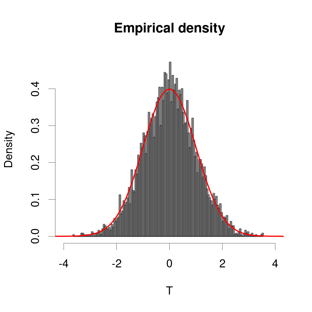
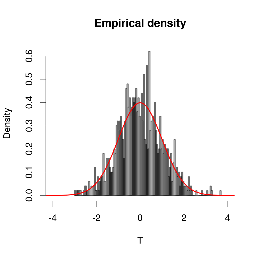
For the model without noise, under the null hypothesis, we also investigate the asymptotic normality of the proposed testing statistics, as shown in Figure 1. The empirical powers under alternative hypothesis HA​2H_{A2} are displayed in Table 3. The results are similar to those under HA​1H_{A1}.

Refer to caption
Refer to caption
Figure 1: Empirical densities for the proposed testing statistics under the null hypothesis when T=p=q=100T=p=q=100. The red real lines correspond to the standard normal density. Left: Normal distribution; Right: Bernoulli distribution.
Table 3: Empirical powers of different testing procedures under the alternative hypothesis HA​2H_{A2} with various pp and TT.
α=0.05\alpha=0.05 α=0.10\alpha=0.10
family p⁡(q)p(q) TT 𝒯F​O\mathcal{T}_{FO} 𝒯B​G\mathcal{T}_{BG} 𝒯B​E\mathcal{T}_{BE} 𝒯F​O\mathcal{T}_{FO} 𝒯B​G\mathcal{T}_{BG} 𝒯B​E\mathcal{T}_{BE}
Normal 20 20 0.179 0.061 0.063 0.267 0.115 0.115
20 60 0.594 0.077 0.432 0.695 0.151 0.547
20 100 0.929 0.487 0.845 0.952 0.615 0.919
100 20 0.979 0.807 0.948 0.993 0.882 0.971
100 60 1 0.997 1 1 0.999 1
100 100 1 1 1 1 1 1
Bernoulli 20 20 0.137 0.064 0.086 0.223 0.119 0.161
20 60 0.586 0.071 0.491 0.704 0.153 0.633
20 100 0.973 0.587 0.947 0.983 0.729 0.976
100 20 0.980 0.818 0.962 0.992 0.895 0.984
100 60 1 0.999 1 1 1 1
100 100 1 1 1 1 1 1

B.2 Dependence on the separable assumption

The proposed testing procedure depends heavily on the separable model (3). The separability may not hold even if cov​{Vec​(𝐘)}\text{cov}\{\text{Vec}(\mathbf{Y})\} has a Kronecker product form, i.e., 𝚺𝐕⊗𝚺𝐔\bm{\Sigma}_{\mathbf{V}}\otimes\bm{\Sigma}_{\mathbf{U}}. Therefore, in this subsection. we investigate the limiting distribution of the proposed testing statistic without the separable assumption. For the data, we let

Vec​(𝐘t)​∼i.i.d.​ℳ​𝒱​(𝟎,𝚺),\text{Vec}(\mathbf{Y}_{t})\overset{i.i.d.}{\sim}\mathcal{MV}({\bf 0},\bm{\Sigma}),

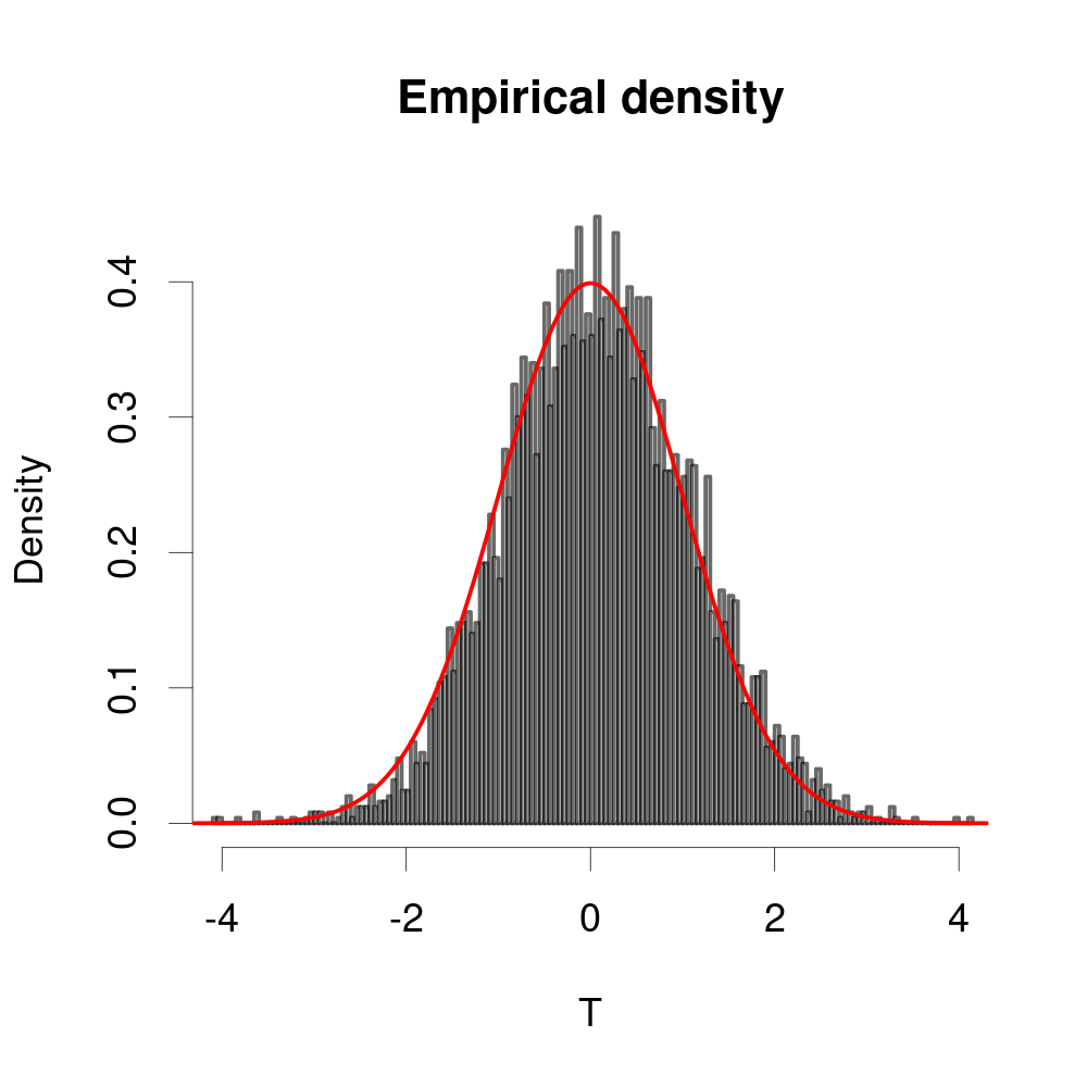
where ℳ​𝒱​(𝟎,𝚺)\mathcal{MV}({\bf 0},\bm{\Sigma}) stands for some multivariate distribution with mean 𝟎{\bf 0} and covariance matrix 𝚺=𝚺𝐕⊗𝚺𝐔\bm{\Sigma}=\bm{\Sigma}_{\mathbf{V}}\otimes\bm{\Sigma}_{\mathbf{U}}. 𝚺𝐔\bm{\Sigma}_{\mathbf{U}} and 𝚺𝐕\bm{\Sigma}_{\mathbf{V}} are the same as those in Table 1 of the main paper. We reshape Vec​(𝐘t)\text{Vec}(\mathbf{Y}_{t}) to p×qp\times q matrix column by column, and use the proposed procedure to calculate the testing statistic with f⁡(x)=x2f(x)=x^{2}. Figure 2 plots the empirical densities when 𝐘t\mathbf{Y}_{t} are from multivariate Gaussian and multivariate tt distribution with degree of freedom equal to 8. For better comparison, we further present the empirical Cumulative Distribution Function (CDF) of the testing statistics in Table 4, together with the quantiles and CDF of standard normal distribution. The results are based on 1000 replications with T=p=q=60T=p=q=60.

Refer to caption
Refer to caption
Figure 2: Empirical densities for the proposed testing statistics without separable assumption but cov​{Vec​(𝐘t)}=𝚺𝐕⊗𝚺𝐔\text{cov}\{\text{Vec}(\mathbf{Y}_{t})\}=\bm{\Sigma}_{\mathbf{V}}\otimes\bm{\Sigma}_{\mathbf{U}}. Left: multivariate Gaussian; Right: multivariate tt. The red real line is the density of standard normal distribution.
Table 4: Standard normal quantiles (Ψ⁡(α)\Psi(\alpha)) and the corresponding empirical cumulative functions of the testing statistics.
Ψ⁡(α)\Psi(\alpha) -1.645 -1.282 -1.036 -0.842 -0.675 -0.524 -0.385 -0.253 -0.126 0.000
α\alpha 0.050 0.100 0.150 0.200 0.250 0.300 0.350 0.400 0.450 0.500
Gaussian 0.051 0.096 0.143 0.201 0.242 0.309 0.361 0.412 0.467 0.514
tt 1 1 1 1 1 1 1 1 1 1
Ψ⁡(α)\Psi(\alpha) 0.126 0.253 0.385 0.524 0.675 0.842 1.036 1.282 1.645
α\alpha 0.550 0.600 0.650 0.700 0.750 0.800 0.850 0.900 0.950
Gaussian 0.563 0.607 0.654 0.707 0.759 0.802 0.852 0.898 0.948
tt 1 1 1 1 1 1 1 1 1

By Figure 2 and Table 6, the testing procedure still works for Gaussian settings but losses effectiveness under tt distribution. Actually, under Gaussian settings, the assumptions of separability and Kronecker product covariance structure are equivalent. After the transformation 𝐘~t=𝚺𝐔−1/2𝐘t\tilde{\mathbf{Y}}_{t}=\bm{\Sigma}_{\mathbf{U}}^{-1/2}\mathbf{Y}_{t}, each column of 𝐘~t\tilde{\mathbf{Y}}_{t} will have covariance matrix equal to 𝐈p\mathbf{I}_{p} while each row of 𝐘~t\tilde{\mathbf{Y}}_{t} will have covariance matrix equal to 𝚺𝐕\bm{\Sigma}_{\mathbf{V}}. When the entries are Gaussian, we can write 𝐘~t=𝑑𝐙t𝚺𝐕−1/2\tilde{\mathbf{Y}}_{t}\overset{d}{=}\mathbf{Z}_{t}\bm{\Sigma}_{\mathbf{V}}^{-1/2}, where the entries of 𝐙t\mathbf{Z}_{t} are from i.i.d. 𝒩⁡(0,1)\mathcal{N}(0,1). When the entries are not from Gaussian, the equivalence will not hold anymore. Under such cases, limiting distributions of linear spectral statistics will depend on not only second-order information of the data, but also higher-order correlations between the entries of 𝐘~t\tilde{\mathbf{Y}}_{t}. Therefore, there can be great shifts both on the asymptotic mean and variance, which is justified by the simulation results with tt distribution.

As a conclusion, the proposed procedure can be used to directly test Kronecker product covariance matrix if the data are from Gaussian. Otherwise, we need to assume separability or specify higher-order correlations in order to remove the Gaussian assumption.

B.3 Model with noise

This part investigates the empirical performance of our testing procedure for the noised model, corresponding to Section 6 of the main paper. We generate independent samples according to model (15) with σα=σβ=1\sigma_{\alpha}=\sigma_{\beta}=1, while the entries of 𝐗t\mathbf{X}_{t}, φt\varphi_{t} and 𝚽t\bm{\Phi}_{t} are all from standard normal or Bernoulli distribution. Considering the identification condition in Lemma 3, we let 𝐔=𝐃1​𝚪1\mathbf{U}=\mathbf{D}_{1}\bm{\Gamma}_{1} and 𝐕=𝐃2​𝚪2\mathbf{V}=\mathbf{D}_{2}\bm{\Gamma}_{2}, where 𝐃1\mathbf{D}_{1}, 𝐃2\mathbf{D}_{2} are diagonal matrices and 𝚪1\bm{\Gamma}_{1}, 𝚪2\bm{\Gamma}_{2} are orthogonal matrices. The spectral distributions of 𝐃12\mathbf{D}_{1}^{2} and 𝐃22\mathbf{D}_{2}^{2} are 0.5​δ1−c1+0.5​δ1+c10.5\delta_{1-c_{1}}+0.5\delta_{1+c_{1}} and 0.5​δ1−c2+0.5​δ1+c20.5\delta_{1-c_{2}}+0.5\delta_{1+c_{2}}, respectively for some constants c1,c2∈(0,1)c_{1},c_{2}\in(0,1). When c1,c2c_{1},c_{2} are small, 𝚺𝐔\bm{\Sigma}_{\mathbf{U}} and 𝚺𝐕\bm{\Sigma}_{\mathbf{V}} will be close to identity matrices, and it’s harder to identify the individual noises from the system. The simulations results below are all based on 1000 replications if not specified separately.

Refer to caption
Refer to caption
Figure 3: Average estimation error ln⁡|σ^β2−σβ2|\ln|\hat{\sigma}_{\beta}^{2}-\sigma_{\beta}^{2}|. Left: c1=c2=0.5c_{1}=c_{2}=0.5 while T=p=qT=p=q. Right: T=p=q=100T=p=q=100 while c1=c2=δc_{1}=c_{2}=\delta.
Refer to caption
Refer to caption
Figure 4: Empirical densities for the proposed testing statistics under the null hypothesis and noised model. The red real lines correspond to the standard normal density. Left: Normal distribution; Right: Bernoulli distribution.

Our first experiment is to study the estimation of σβ2\sigma_{\beta}^{2}, which plays an important role in the normalization step. Figure 3 shows the average absolute estimation error after log transformation (ln⁡|σ^β2−σβ2|\ln|\hat{\sigma}_{\beta}^{2}-\sigma_{\beta}^{2}|) under different settings. As shown in the left panel, the estimation error decreases as the dimension and sample size grow. The two lines have scope smaller than −1.5-1.5, which implies that the convergence rate of σ^β2\hat{\sigma}_{\beta}^{2} can be even faster than that in Lemma 3. The right panel indicates that σβ2\sigma_{\beta}^{2} can be estimated more accurately when it’s easier to identify the individual noises, as expected.

Our second experiment is to verify the asymptotic distribution in Theorem 5. We fix T=p=q=100T=p=q=100 and c1=0.5c_{1}=0.5, c2=0.8c_{2}=0.8. Figure 4 shows the histograms of the normalized testing statistics, σ~−1​{tr​(𝒮¯2−μ~)}\tilde{\sigma}^{-1}\{\text{tr}(\bar{\mathcal{S}}^{2}-\tilde{\mu})\}, over 5000 replications. It’s clear that the empirical densities are close to normal density under the two distribution families.

Our third experiment is to verify the empirical sizes of the proposed testing statistics under the null. We will also investigate the effects of the estimation error for unknown parameters. When all the unknown parameters (σβ\sigma_{\beta}, 𝚺𝐕\bm{\Sigma}_{\mathbf{V}}, ν4\nu_{4} and ν~4\tilde{\nu}_{4}) are given, we denote the results by 𝒯F​G\mathcal{T}_{FG}, meaning “Fully Given”. On the contrary, if all the unknown parameters are estimated by the arguments in Section A, we denote the results by 𝒯F​E\mathcal{T}_{FE}, meaning “Fully Estimated”. Moreover, note that the estimation of σ^β2\hat{\sigma}_{\beta}^{2} mainly affects the normalization matrix ℰ0\mathcal{E}_{0}. Therefore, we further construct a testing statistic where ℰ0\mathcal{E}_{0} is estimated with σβ2\sigma_{\beta}^{2} given, denoted by 𝒯P​G\mathcal{T}_{PG}, meaning “Partially Given”. The empirical sizes of the three testing statistics are presented in Table 5. It’s seen that when T,p,qT,p,q are sufficiently large, our testing statistics have well-controlled sizes no matter the unknown parameters are given or estimated. Comparing 𝒯F​E\mathcal{T}_{FE} and 𝒯P​G\mathcal{T}_{PG}, we conclude that when T,p,qT,p,q are small, the testing statistic may lose effectiveness mainly because the estimated σβ2\sigma_{\beta}^{2} is not accurate, which is understandable by Lemma 3.

Table 5: Empirical sizes of different testing statistics under the null hypothesis and noised model, with various pp and TT.
α=0.05\alpha=0.05 α=0.10\alpha=0.10
family p⁡(q)p(q) TT 𝒯F​G\mathcal{T}_{FG} 𝒯F​E\mathcal{T}_{FE} 𝒯P​G\mathcal{T}_{PG} 𝒯F​G\mathcal{T}_{FG} 𝒯F​E\mathcal{T}_{FE} 𝒯P​G\mathcal{T}_{PG}
Normal 20 20 0.076 0.632 0.059 0.140 0.699 0.103
20 60 0.063 0.218 0.065 0.121 0.304 0.117
20 100 0.049 0.124 0.047 0.109 0.194 0.101
60 20 0.061 0.196 0.055 0.110 0.275 0.118
60 60 0.048 0.071 0.048 0.091 0.139 0.106
60 100 0.041 0.054 0.044 0.082 0.113 0.096
100 20 0.078 0.115 0.070 0.146 0.188 0.101
100 60 0.065 0.060 0.055 0.101 0.122 0.101
100 100 0.041 0.047 0.050 0.094 0.097 0.085
Bernoulli 20 20 0.062 0.387 0.044 0.104 0.469 0.091
20 60 0.050 0.099 0.052 0.094 0.156 0.096
20 100 0.039 0.061 0.035 0.081 0.104 0.079
60 20 0.068 0.089 0.052 0.112 0.154 0.106
60 60 0.050 0.044 0.042 0.099 0.105 0.092
60 100 0.051 0.055 0.053 0.104 0.101 0.100
100 20 0.074 0.066 0.059 0.124 0.124 0.110
100 60 0.055 0.051 0.048 0.099 0.101 0.101
100 100 0.053 0.051 0.051 0.101 0.090 0.093

Our last experiment is to investigate the empirical powers under alternative hypotheses. Similarly to the model without noise, we consider two types of alternative hypotheses. For HA​1H_{A1}, we let 𝐔=𝐃1​𝚪1+β1​𝜸​𝜸′/p\mathbf{U}=\mathbf{D}_{1}\bm{\Gamma}_{1}+\beta_{1}\bm{\gamma}\bm{\gamma}^{\prime}/\sqrt{p}, where 𝜸\bm{\gamma} is the pp-dimensional vector whose entries are from i.i.d. 𝒩⁡(0,1)\mathcal{N}(0,1). For HA​2H_{A2}, we let 𝐔=(𝐃1+β2​𝐈p)​𝚪1\mathbf{U}=(\mathbf{D}_{1}+\beta_{2}\mathbf{I}_{p})\bm{\Gamma}_{1}. In the simulations, β1=β2=0.1\beta_{1}=\beta_{2}=0.1. The empirical sizes of 𝒯F​G\mathcal{T}_{FG}, 𝒯F​E\mathcal{T}_{FE} and 𝒯P​G\mathcal{T}_{PG} under HA​1H_{A1} and HA​2H_{A2} are shown in Table 6 and Table 7, respectively. We conclude that the empirical powers are pretty strong as long as T,p,qT,p,q are large.

Table 6: Empirical powers of different testing statistics under the noised model and alternative hypothesis HA​1H_{A1}, with various pp and TT.
α=0.05\alpha=0.05 α=0.10\alpha=0.10
family p⁡(q)p(q) TT 𝒯F​G\mathcal{T}_{FG} 𝒯F​E\mathcal{T}_{FE} 𝒯P​G\mathcal{T}_{PG} 𝒯F​G\mathcal{T}_{FG} 𝒯F​E\mathcal{T}_{FE} 𝒯P​G\mathcal{T}_{PG}
Normal 20 20 0.705 0.921 0.623 0.770 0.948 0.713
20 100 0.995 0.995 0.995 0.997 0.997 0.996
100 20 0.911 0.917 0.869 0.941 0.955 0.914
100 100 1 1 1 1 1 1
Bernoulli 20 20 0.160 0.635 0.157 0.227 0.703 0.236
20 100 0.918 0.930 0.907 0.947 0.962 0.947
100 20 1 1 1 1 1 1
100 100 1 1 1 1 1 1
Table 7: Empirical powers of different testing statistics under the noised model and alternative hypothesis HA​2H_{A2}, with various pp and TT.
α=0.05\alpha=0.05 α=0.10\alpha=0.10
family p⁡(q)p(q) TT 𝒯F​G\mathcal{T}_{FG} 𝒯F​E\mathcal{T}_{FE} 𝒯P​G\mathcal{T}_{PG} 𝒯F​G\mathcal{T}_{FG} 𝒯F​E\mathcal{T}_{FE} 𝒯P​G\mathcal{T}_{PG}
Normal 20 20 0.919 0.212 0.351 0.944 0.285 0.446
20 100 1 0.863 1 1 0.893 1
100 20 1 0.917 1 1 0.944 1
100 100 1 1 1 1 1 1
Bernoulli 20 20 0.942 0.121 0.310 0.962 0.173 0.424
20 100 1 0.975 1 1 0.985 1
100 20 1 0.980 1 1 0.989 1
100 100 1 1 1 1 1 1

Appendix C Real data analysis

In this section, we analyze a real data set. The data set consists of monthly returns of 100 portfolios, which can be freely downloaded from http://mba.tuck.dartmouth.edu/pages/faculty/ken.french/data_library.html. The portfolios can be further categorized into 10 levels of capital sizes and 10 levels of book-to-equity ratios. Hence, it’s naturally structured as 10×1010\times 10 matrix-variate series, also known as the Fama-French 10×1010\times 10 portfolios. Considering the missing rate, we only use the data from January-1964 to December-2020, with a total of 684 months. We impute the missing values (missing rate is 0.25%0.25\%) by linear interpolation. The data set was ever analyzed in Wang et al. 2019 and Yu et al. 2021. Following their preprocessing procedures, we first subtract the monthly market excess returns and then standardize the series one by one. Figure 5 is an illustration of the standardized series.
Refer to caption
Figure 5: Standardized Fama-French 10×1010\times 10 portfolio series. Each series is associated with a level of capital size and a level of book-to-equity ratio. Top to bottom: lower book-to-equity ratio to higher. Left to right: small capital size to larger.

We start with the model (3) without noise, which assumes a Kronecker product covariance structure for the 10×1010\times 10 matrices. We first provide some initial guesses of the row-row and column-column covariance matrices 𝚺𝐔\bm{\Sigma}_{\mathbf{U}} and 𝚺𝐕\bm{\Sigma}_{\mathbf{V}}. The target of this study is to select the most convincing one. Since the sample size is much larger than dimensions, it’s natural to consider the sample versions

𝚺𝐔1=16840​∑t=1684𝐘t​𝐘t′,𝚺𝐕1=16840​∑t=1684𝐘t′​𝐘t,\bm{\Sigma}_{\mathbf{U}_{1}}=\frac{1}{6840}\sum_{t=1}^{684}\mathbf{Y}_{t}\mathbf{Y}_{t}^{\prime},\quad\bm{\Sigma}_{\mathbf{V}_{1}}=\frac{1}{6840}\sum_{t=1}^{684}\mathbf{Y}_{t}^{\prime}\mathbf{Y}_{t},

which are actually unbiased estimators respectively under the identification conditions tr​(𝚺𝐕)/10=1\text{tr}(\bm{\Sigma}_{\mathbf{V}})/10=1 and tr​(𝚺𝐔)/10=1\text{tr}(\bm{\Sigma}_{\mathbf{U}})/10=1. Although the two identification conditions may not hold simultaneously, it has no effects on this study since we will test 𝚺𝐔\bm{\Sigma}_{\mathbf{U}} and 𝚺𝐕\bm{\Sigma}_{\mathbf{V}} separately. We plot 𝚺𝐔1\bm{\Sigma}_{\mathbf{U}_{1}}, 𝚺𝐕1\bm{\Sigma}_{\mathbf{V}_{1}}, their inverse matrices and eigenvalues in Figure 6.

Refer to caption
(a) heatmap of 𝚺^𝐔1\hat{\bm{\Sigma}}_{\mathbf{U}_{1}}
Refer to caption
(b) heatmap of 𝚺^𝐔1−1\hat{\bm{\Sigma}}_{\mathbf{U}_{1}}^{-1}
Refer to caption
(c) Eigenvalues of 𝚺^𝐔1\hat{\bm{\Sigma}}_{\mathbf{U}_{1}}
Refer to caption
(d) heatmap of 𝚺^𝐕1\hat{\bm{\Sigma}}_{\mathbf{V}_{1}}
Refer to caption
(e) heatmap of 𝚺^𝐕1−1\hat{\bm{\Sigma}}_{\mathbf{V}_{1}}^{-1}
Refer to caption
(f) Eigenvalues of 𝚺^𝐕1\hat{\bm{\Sigma}}_{\mathbf{V}_{1}}
Figure 6: Sample covariances 𝚺^𝐔1\hat{\bm{\Sigma}}_{\mathbf{U}_{1}}, 𝚺^𝐕1\hat{\bm{\Sigma}}_{\mathbf{V}_{1}}, their inverses and corresponding eigenvalues.

By Figure 6, the largest eigenvalues of 𝚺𝐔1\bm{\Sigma}_{\mathbf{U}_{1}} and 𝚺𝐕1\bm{\Sigma}_{\mathbf{V}_{1}} are well separated from the others. This indicates a potential low-rank plus noise structure, which is motivated by the matrix-valued factor models ever studied in Wang et al. 2019 and Yu et al. 2021. Then, we construct factor-based guess of 𝚺𝐔2\bm{\Sigma}_{\mathbf{U}_{2}} by

𝚺𝐔2=∑j=1kλj​(𝚺𝐔1)​𝝃j​𝝃j′+diag​(𝚿),\bm{\Sigma}_{\mathbf{U}_{2}}=\sum_{j=1}^{k}\lambda_{j}(\bm{\Sigma}_{\mathbf{U}_{1}})\bm{\xi}_{j}\bm{\xi}_{j}^{\prime}+\text{diag}(\bm{\Psi}),

where 𝝃j\bm{\xi}_{j} is the jj-th eigenvector of 𝚺𝐔1\bm{\Sigma}_{\mathbf{U}_{1}} and 𝚿=𝚺𝐔1−∑j=1kλj​(𝚺𝐔1)​𝝃j​𝝃j′\bm{\Psi}=\bm{\Sigma}_{\mathbf{U}_{1}}-\sum_{j=1}^{k}\lambda_{j}(\bm{\Sigma}_{\mathbf{U}_{1}})\bm{\xi}_{j}\bm{\xi}_{j}^{\prime}. Motivated by the “POET” estimator in Fan et al. 2013, diag​(𝚿)\text{diag}(\bm{\Psi}) can be replaced by penalized versions, e.g., using the hard-thresholding technique in Bickel and Levina 2008a. In this example, we use diag​(𝚿)\text{diag}(\bm{\Psi}) for simplicity. We let k=5k=5 so that the leading factors can explain over 75%75\% variance of 𝚺𝐔1\bm{\Sigma}_{\mathbf{U}_{1}}. Similar procedure leads to a modified version of 𝚺𝐕\bm{\Sigma}_{\mathbf{V}}, denoted by 𝚺𝐕2\bm{\Sigma}_{\mathbf{V}_{2}}. Figure 6 also shows that 𝚺𝐔1−1\bm{\Sigma}_{\mathbf{U}_{1}}^{-1} and 𝚺𝐕1−1\bm{\Sigma}_{\mathbf{V}_{1}}^{-1} seem to be sparse. Hence, motivated by Zhou 2014, it’s reasonable to consider the graphical-lasso estimator, defined by

𝛀g​l=argmin𝛀>0(tr(𝚺𝐔1𝛀)−logdet(𝛀)+λ|𝛀|1,off),\bm{\Omega}_{gl}=\arg\min_{\bm{\Omega}>0}\bigg(\text{tr}(\bm{\Sigma}_{\mathbf{U}_{1}}\bm{\Omega})-\log\det(\bm{\Omega})+\lambda|\bm{\Omega}|_{1,\text{off}}\bigg),

where λ\lambda is a tuning parameter. We let λ=0.05\lambda=0.05 in this example for comparison. Then, the graphical-lasso based guess of 𝚺𝐔\bm{\Sigma}_{\mathbf{U}} is 𝚺𝐔3:=𝛀g​l−1\bm{\Sigma}_{\mathbf{U}_{3}}:=\bm{\Omega}_{gl}^{-1}. Similar technique can be applied to 𝚺𝐕1\bm{\Sigma}_{\mathbf{V}_{1}} to obtain 𝚺𝐕3\bm{\Sigma}_{\mathbf{V}_{3}}.

Currently we have three preliminary guesses for 𝚺𝐔\bm{\Sigma}_{\mathbf{U}} and 𝚺𝐕\bm{\Sigma}_{\mathbf{V}}. In portfolio theory, the covariance matrix is critical to finding the risk-minimization investing strategy, which is equivalent to solving the optimization problem

𝒘o​p=arg⁡min‖𝒘‖=1​var​(𝒘′​Vec​(𝐘))=𝚺𝐘−1​𝟏𝟏′​𝚺𝐘−1​𝟏,\bm{w}_{op}=\arg\min_{\|\bm{w}\|=1}\text{var}\bigg(\bm{w}^{\prime}\text{Vec}(\mathbf{Y})\bigg)=\frac{\bm{\Sigma}_{\mathbf{Y}}^{-1}{\bf 1}}{{\bf 1}^{\prime}\bm{\Sigma}_{\mathbf{Y}}^{-1}{\bf 1}},

where 𝚺𝐘=Cov​{Vec​(𝐘)}\bm{\Sigma}_{\mathbf{Y}}=\text{Cov}\{\text{Vec}(\mathbf{Y})\} and 𝟏{\bf 1} is a vector with entries all being 1. 𝒘^\hat{\bm{w}} determines the best weights assigned to Vec​(𝐘)\text{Vec}(\mathbf{Y}). Then, based on the preliminary guesses, taking 𝚺𝐘=𝚺𝐕⊗𝚺𝐔\bm{\Sigma}_{\mathbf{Y}}=\bm{\Sigma}_{\mathbf{V}}\otimes\bm{\Sigma}_{\mathbf{U}}, we calculate the risk-minimization portfolio weights and report them in Figure 7. 𝒘o​p\bm{w}_{op} is restructured into 10×1010\times 10 matrices for better representation.

1.9 1.4 1.2 1.1 1.5 1.5 1.6 1.8 1.6 1.9
0.8 0.5 0.5 0.4 0.6 0.6 0.6 0.7 0.6 0.7
0.5 0.3 0.3 0.3 0.4 0.4 0.4 0.4 0.4 0.5
0.9 0.6 0.5 0.5 0.7 0.7 0.7 0.8 0.7 0.9
0.7 0.5 0.5 0.4 0.6 0.6 0.6 0.7 0.6 0.7
0.9 0.6 0.5 0.5 0.6 0.7 0.7 0.8 0.7 0.8
1.0 0.7 0.6 0.6 0.7 0.7 0.8 0.9 0.8 0.9
1.3 0.9 0.8 0.8 1.0 1.0 1.1 1.3 1.1 1.3
1.8 1.3 1.1 1.1 1.4 1.4 1.5 1.7 1.5 1.8
2.7 1.9 1.7 1.6 2.1 2.1 2.3 2.6 2.3 2.7
(a) 𝒘o​p\bm{w}_{op} from 𝚺𝐕1⊗𝚺𝐔1\bm{\Sigma}_{\mathbf{V}_{1}}\otimes\bm{\Sigma}_{\mathbf{U}_{1}}
3.5 1.9 0.8 0.9 3.1 1.8 2.5 3.3 1.9 3.0
0.5 0.3 0.1 0.1 0.5 0.3 0.4 0.5 0.3 0.5
-0.2 -0.1 0.0 0.0 -0.2 -0.1 -0.1 -0.2 -0.1 -0.2
0.5 0.3 0.1 0.1 0.4 0.3 0.4 0.5 0.3 0.4
-0.1 -0.1 0.0 0.0 -0.1 -0.1 -0.1 -0.1 -0.1 -0.1
1.8 1.0 0.4 0.5 1.6 0.9 1.3 1.7 1.0 1.5
1.0 0.5 0.2 0.3 0.9 0.5 0.7 1.0 0.6 0.9
2.4 1.3 0.6 0.6 2.1 1.2 1.7 2.3 1.3 2.0
2.3 1.2 0.5 0.6 2.0 1.2 1.6 2.2 1.3 1.9
3.8 2.0 0.9 0.9 3.3 1.9 2.6 3.5 2.0 3.2
(b) 𝒘o​p\bm{w}_{op} from 𝚺𝐕2⊗𝚺𝐔2\bm{\Sigma}_{\mathbf{V}_{2}}\otimes\bm{\Sigma}_{\mathbf{U}_{2}}
1.6 1.2 1.1 1.1 1.3 1.3 1.4 1.6 1.4 1.6
0.8 0.6 0.6 0.5 0.7 0.7 0.7 0.8 0.7 0.8
0.6 0.4 0.4 0.4 0.5 0.5 0.5 0.6 0.5 0.6
0.9 0.7 0.6 0.6 0.7 0.7 0.8 0.8 0.8 0.9
0.8 0.6 0.5 0.5 0.6 0.6 0.7 0.8 0.7 0.8
0.9 0.7 0.6 0.6 0.7 0.7 0.8 0.9 0.8 0.9
1.0 0.7 0.7 0.6 0.8 0.8 0.8 0.9 0.8 1.0
1.3 0.9 0.9 0.8 1.0 1.0 1.1 1.2 1.1 1.3
1.7 1.2 1.1 1.1 1.3 1.3 1.4 1.6 1.4 1.7
2.4 1.8 1.6 1.6 1.9 2.0 2.1 2.3 2.1 2.4

(c) 𝒘o​p\bm{w}_{op} from 𝚺𝐕3⊗𝚺𝐔3\bm{\Sigma}_{\mathbf{V}_{3}}\otimes\bm{\Sigma}_{\mathbf{U}_{3}}
Refer to caption
(d) historical revenue
Figure 7: (a) to (c): optimal portfolio weights with 𝚺𝐘\bm{\Sigma}_{\mathbf{Y}} from three estimators. All the values have been multiplied by 100 for better representation. (d): historical revenue of corresponding portfolio weights regardless of liquidity and transaction fees.

It’s seen from Figure 7 that the optimal portfolio weights can vary a lot when 𝚺𝐘\bm{\Sigma}_{\mathbf{Y}} is estimated by different methods. For the factor-based 𝒘^2\hat{\bm{w}}_{2}, it assigns negative weights to some portfolios, referring to “short” strategy which are contradictory to the other two methods. It’s then of importance to determine which strategy is more convincing. Empirically, the historical revenues of different strategies can provide a criterion to select the best one. However, in this example, the historical revenue curve of the three strategies are so close to each other, as displayed in Figure 7 (d). In the below, we apply the proposed testing procedure to select the most convincing strategy, i.e., to select the covariance matrix nearest to the truth.

We use the testing algorithm 1 to test 𝚺𝐔=𝚺𝐔0\bm{\Sigma}_{\mathbf{U}}=\bm{\Sigma}_{\mathbf{U}_{0}}, where 𝚺𝐔0\bm{\Sigma}_{\mathbf{U}_{0}} is any of the above preliminary guess. We clarify here that when saying “testing”, we regard 𝚺𝐔0\bm{\Sigma}_{\mathbf{U}_{0}} as a given constant matrix, but not an estimator. The unknown parameters in the testing statistics are estimated by the procedure illustrated in Section 4.3. This leads to the testing statistics 𝒯1=30.15\mathcal{T}_{1}=30.15, 𝒯2=184.23\mathcal{T}_{2}=184.23 and 𝒯3=129.31\mathcal{T}_{3}=129.31, associated with 𝚺𝐔1\bm{\Sigma}_{\mathbf{U}_{1}}, 𝚺𝐔2\bm{\Sigma}_{\mathbf{U}_{2}} and 𝚺𝐔3\bm{\Sigma}_{\mathbf{U}_{3}} respectively. That is, all the preliminary guesses of 𝚺𝐔\bm{\Sigma}_{\mathbf{U}} are rejected significantly, which is common in real examples because the model can be misspecified. However, a larger deviation from the interval [−2,2][-2,2] usually indicates more significant rejection. Hence, in this example, it’s more recommended to believe in the sample covariance matrix 𝚺𝐔1\bm{\Sigma}_{\mathbf{U}_{1}}. This is partially rationalized by the large sample size of this data set. Actually, if we select the tuning parameter λ\lambda of the graphical lasso estimator by cross validation, it always leads to λ=0\lambda=0, which is exactly associated with the sample covariance matrix. It’s also standard in the literature to test where the covariance matrix is an scaled identity matrix, i.e., 𝚺𝐔=𝐈×tr​(𝚺𝐔1)/10\bm{\Sigma}_{\mathbf{U}}=\mathbf{I}\times\text{tr}(\bm{\Sigma}_{\mathbf{U}_{1}})/10. This leads to a testing statistic 𝒯4=212.69\mathcal{T}_{4}=212.69, which deviates most significantly from the interval [−2,2][-2,2]. In other words, the preliminary guesses 𝚺𝐔1\bm{\Sigma}_{\mathbf{U}_{1}}, 𝚺𝐔2\bm{\Sigma}_{\mathbf{U}_{2}} and 𝚺𝐔3\bm{\Sigma}_{\mathbf{U}_{3}} work at least better than a simple guess of identity matrix. For 𝚺𝐕\bm{\Sigma}_{\mathbf{V}}, a parallel procedure is applied to the series {𝐘t′}t=1684\{\mathbf{Y}_{t}^{\prime}\}_{t=1}^{684}, which leads to testing statistics 𝒯1=35.67\mathcal{T}_{1}=35.67, 𝒯2=280.70\mathcal{T}_{2}=280.70 and 𝒯3=137.96\mathcal{T}_{3}=137.96. The hypothesis 𝚺𝐕=𝐈×tr​(𝚺𝐕1)/10\bm{\Sigma}_{\mathbf{V}}=\mathbf{I}\times\text{tr}(\bm{\Sigma}_{\mathbf{V}_{1}})/10 will lead to 𝒯4=223.64\mathcal{T}_{4}=223.64. Therefore, the sample covariance matrix estimator 𝚺𝐕1\bm{\Sigma}_{\mathbf{V}_{1}} is still the most convincing one in this example.

Next, we consider the noised model (15) for this real example. Using the procedure in Section 6, we have σ^β2=0.47\hat{\sigma}_{\beta}^{2}=0.47. Then, we remove the common noise from the model and obtain {𝐘^t}\{\hat{\mathbf{Y}}_{t}\}. Left and middle panels of Figure 8 plot the eigenvalues of the sample covariance matrices 𝚺𝐔1\bm{\Sigma}_{\mathbf{U}_{1}} and 𝚺𝐕1\bm{\Sigma}_{\mathbf{V}_{1}} from {𝐘t}\{\mathbf{Y}_{t}\}. Compared with Figure 6, the eigenvalues now decay more smoothly, and no significantly spiked eigenvalues are found.
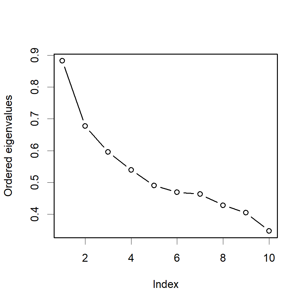
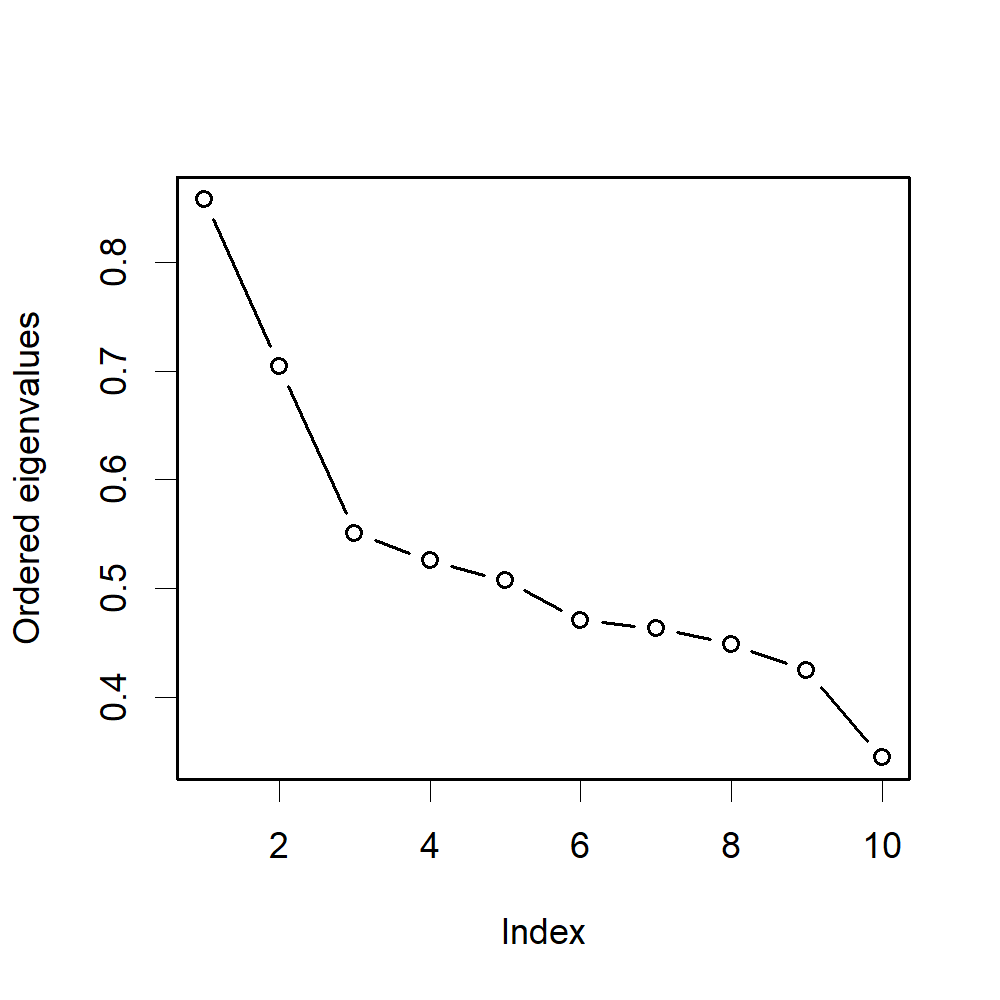
Refer to caption
Refer to caption
Refer to caption
Figure 8: Eigenvalues of the sample covariance matrices 𝚺𝐔1\bm{\Sigma}_{\mathbf{U}_{1}}, 𝚺𝐕1\bm{\Sigma}_{\mathbf{V}_{1}} from {𝐘t}\{\mathbf{Y}_{t}\}, and Re​(Ω)\text{Re}(\Omega), under noised model.

In the next step, we calculate the reshaped matrix Re​(Ω^)\text{Re}(\hat{\Omega}) according to the definition in the main paper. Right panel of Figure 8 shows the eigenvalues of Re​(Ω^)\text{Re}(\hat{\Omega}). According to our proof of Lemma 3 and the arguments in Section 8, Re​(Ω^)\text{Re}(\hat{\Omega}) should have two spiked eigenvalues if σβ2≥c\sigma_{\beta}^{2}\geq c for some constant c>0c>0, which is not observed in the figure. Therefore, we conclude that either σβ2=0\sigma_{\beta}^{2}=0 or the identification condition in Lemma 3 does not hold. Under such cases, it’s more meaningful to test 𝚺𝐔\bm{\Sigma}_{\mathbf{U}} and σβ2\sigma_{\beta}^{2} jointly. In this example, we test the null hypothesis that 𝚺𝐔=𝚺𝐔1\bm{\Sigma}_{\mathbf{U}}=\bm{\Sigma}_{\mathbf{U}_{1}} and σβ2=0\sigma_{\beta}^{2}=0 hold simultaneously. This leads to testing statistic equal to −23.58-23.58. Compared with the model without noise, the new testing statistic deviates less from the interval [−2,2][-2,2], which benefits mainly from the existence of common noise. A parallel procedure for 𝚺𝐕\bm{\Sigma}_{\mathbf{V}} leads to testing statistic equal to −34.55-34.55 and similar conclusion holds.

Appendix D Outline of the proof

The major target of Sections D to H is to prove the CLT of LSS in Theorem 1 of the main paper. We first give two lemmas concerning the spectral properties of S¯p\bar{S}_{p}.

Lemma 7 (Wang and Paul 2014).

Suppose that Condition 1 holds. Then the empirical spectral distribution of S¯p\bar{S}_{p} almost surely converges to a non-random probability function FF whose Stieltjes transform m⁡(z)m(z) is the unique solution satisfying ℑ⁡m⁡(z)>0\Im m(z)>0 and

m(z)=−∫1z+x​λ¯B2​s​(z)dFA(x),s(z)=−∫xz+x​λ¯B2​s​(z)dFA(x),z∈ℂ+.m(z)=-\int\frac{1}{z+x\bar{\lambda}_{B^{2}}s(z)}dF^{A}(x),\quad s(z)=-\int\frac{x}{z+x\bar{\lambda}_{B^{2}}s(z)}dF^{A}(x),\quad z\in\mathbb{C}^{+}. (20)

where λ¯B2=limn→∞n−1​tr​(Bn2)=∫x2​d​FB​(x)\bar{\lambda}_{B^{2}}=\lim_{n\rightarrow\infty}n^{-1}\text{tr}(B_{n}^{2})=\int x^{2}dF^{B}(x) is a positive constant.

Lemma 8 (Bound on ‖S¯p‖\|\bar{S}_{p}\|).

Suppose that Condition 1 holds. Then the spectral norm of S¯p\bar{S}_{p} satisfies ‖S¯p‖≤2​limsuppa1​b1\|\bar{S}_{p}\|\leq 2\lim\sup_{p}a_{1}b_{1} almost surely.

Lemma 7 is borrowed from Wang and Paul 2014, while the proof of Lemma 8 is in the next section. Indeed, mp​(z)m_{p}(z) and sp​(z)s_{p}(z) in the main paper are finite sample versions of m⁡(z)m(z) and s⁡(z)s(z), respectively. Recall the definition

G~p​(f)=p​∫−∞+∞f⁡(x)​d​(FS¯p​(x)−Fp​(x)),\tilde{G}_{p}(f)=p\int_{-\infty}^{+\infty}f(x)d(F^{\bar{S}_{p}}(x)-F_{p}(x)),

where f∈ℳ={functions which are analytic in an open domain containing​[−2​c,2​c]}f\in\mathcal{M}=\{\text{functions which are analytic in an open domain containing}[-2c,2c]\} with c=limsuppa1​b1c=\lim\sup_{p}a_{1}b_{1}. Define an event Up={∥S¯p∥≤2limsupa1b1}U_{p}=\{\|\bar{S}_{p}\|\leq 2\lim\sup a_{1}b_{1}\}. Then by Lemma 8 and the Cauchy integral formula, UpU_{p} happens with probability tending to one and

G~p(f)=−12​π​i∮𝒞f(z)p{mFS¯p(z)−mp(z)}dz,\tilde{G}_{p}(f)=-\frac{1}{2\pi i}\oint_{\mathcal{C}}f(z)p\{m_{F^{\bar{S}_{p}}}(z)-m_{p}(z)\}dz,

where mFS¯p​(z)m_{F^{\bar{S}_{p}}}(z) and mp​(z)m_{p}(z) are Stieltjes transforms associated with FS¯p​(x)F^{\bar{S}_{p}}(x) and Fp​(x)F_{p}(x) respectively, 𝒞\mathcal{C} is the contour formed by the boundary of the rectangle with four vertices (±u0,±i​v0)(\pm u_{0},\pm iv_{0}) where u0=2​limsuppa1​b1+ϵ0u_{0}=2\lim\sup_{p}a_{1}b_{1}+\epsilon_{0} with sufficiently small ϵ0\epsilon_{0}, and v0v_{0} is any positive number so that ff is analytic in a neighborhood of 𝒞\mathcal{C}. Hence, it’s sufficient to study the Stieltjes transform on the contour 𝒞\mathcal{C}. Our major target is then to prove that with the mean correction term 𝒳p​(z)\mathcal{X}_{p}(z) defined in the main paper, the process

Mp​(z)=p⁡{mFS¯p​(z)−mp​(z)−𝒳p​(z)}M_{p}(z)=p\{m_{F^{\bar{S}_{p}}}(z)-m_{p}(z)-\mathcal{X}_{p}(z)\} (21)

converges weakly to some limit which needs to be specified.

We will start with a simple case where ApA_{p} is diagonal. To avoid dealing with small imaginary part of zz, we denote

𝒞u={u+iv0:u∈[−u0,u0]},𝒞l={−u0+iv:v∈[ηp/p,v0]},𝒞r={u0+iv:v∈[ηp/p,v0]},𝒞0={−u0+iv:v∈[0,ηp/p]}∪{u0+iv:v∈[0,ηp/p]},\begin{split}&\mathcal{C}_{u}=\{u+iv_{0}:u\in[-u_{0},u_{0}]\},\quad\mathcal{C}_{l}=\{-u_{0}+iv:v\in[\eta_{p}/p,v_{0}]\},\\ &\mathcal{C}_{r}=\{u_{0}+iv:v\in[\eta_{p}/p,v_{0}]\},\quad\mathcal{C}_{0}=\{-u_{0}+iv:v\in[0,\eta_{p}/p]\}\cup\{u_{0}+iv:v\in[0,\eta_{p}/p]\},\end{split}

where {ηp}\{\eta_{p}\} is a sequence decreasing to 00 satisfying ηp≥p−α\eta_{p}\geq p^{-\alpha} for some α∈(0,1)\alpha\in(0,1), and v0v_{0} is a constant. The following theorem specifies the limit of the process Mp​(z)M_{p}(z) for z∈𝒞uz\in\mathcal{C}_{u}.

Theorem 7 (Stieltjes transform).

With Condition 1, if ApA_{p} is diagonal, with 𝒳p​(z)\mathcal{X}_{p}(z) defined in the main paper, the process {Mp​(z):z∈𝒞u}\{M_{p}(z):z\in\mathcal{C}_{u}\} converges weakly to a two-dimensional Gaussian process M(⋅)M(\cdot) with mean zero and the covariance function Λ⁡(z1,z2)\Lambda(z_{1},z_{2}), where Λ⁡(z1,z2)\Lambda(z_{1},z_{2}) is defined in Theorem 1.

Therefore, the proof of Theorem 1 is divided into two parts. The first part proves Theorem 7, organized in Sections E to G. The second part is in Section H, which considers contours 𝒞l,r,0\mathcal{C}_{l,r,0} and general 𝐀p\mathbf{A}_{p}. Here we only present some key ideas.

To prove Theorem 7, we decompose Mp​(z)M_{p}(z) into random part and non-random part as follows,

Mp​(z)=p⁡[mF𝐒¯p​(z)−𝔼​mF𝐒¯p​(z)]+p⁡[𝔼​mF𝐒¯p​(z)−mp​(z)−𝒳p​(z)]=Mp​1​(z)+Mp​2​(z).M_{p}(z)=p[m_{F^{\bar{\mathbf{S}}_{p}}}(z)-\mathbb{E}m_{F^{\bar{\mathbf{S}}_{p}}}(z)]+p[\mathbb{E}m_{F^{\bar{\mathbf{S}}_{p}}}(z)-m_{p}(z)-\mathcal{X}_{p}(z)]=M_{p1}(z)+M_{p2}(z).

The random part Mp​1​(z)M_{p1}(z) mainly contributes to the covariance function while the non-random part Mp​2​(z)M_{p2}(z) mainly contributes to the mean correction term 𝒳p​(z)\mathcal{X}_{p}(z).

To deal with Mp​1​(z)M_{p1}(z), we expand the Stieltjes transform and observe that the randomness mainly comes from a sum of martingale in equation (40) below. With the decomposition in this equation, we easily verify the finite-dimensional distribution of Mp​1​(z)M_{p1}(z) and specify the covariance function, following a similar expansion strategy in Chen and Pan 2015. Finally, we finish the proof for Mp​1​(z)M_{p1}(z) by verifying the tightness. The details are put in Section F.

For Mp​2​(z)M_{p2}(z), we first calculate the diagonal entries of Green function with Schur’s complement formula. It’s seen that the diagonal entries will converge to the terms ϵ~k​(z)\tilde{\epsilon}_{k}(z) defined in the main paper. However, the convergence rates are slow, so we need more detailed calculations of the errors to specify those which are not smaller than O⁡(p−1)O(p^{-1}). The proof procedure is more complicated than that in Chen and Pan 2015, where 𝔼​mF𝐒¯P​(z)\mathbb{E}m_{F^{\bar{\mathbf{S}}_{P}}}(z) can be explicitly solved by a quadratic equation of one variable. With general 𝐀p\mathbf{A}_{p} and 𝐁n\mathbf{B}_{n}, we find that the equation therein is not correct anymore. Instead, we expand the diagonal entries of the Stieltjes transform using the inverse matrix formula recursively. After each expansion step, we remove some ”big” errors by rigorous approximation. Finally, we sum up all these non-negligible errors, which lead to the mean correction term 𝒳p​(z)\mathcal{X}_{p}(z).

To complete the proof of Theorem 1, we first prove that the integrals corresponding to 𝒞l,r,0\mathcal{C}_{l,r,0} are negligible. Since the event 𝐔p(ϵ0):={∥𝐒¯p∥≤2limsupa1b1+ϵ0/2}\mathbf{U}_{p}(\epsilon_{0}):=\{\|\bar{\mathbf{S}}_{p}\|\leq 2\lim\sup a_{1}b_{1}+\epsilon_{0}/2\} happens with probability tending to 1 for large pp, we aim to prove that under this event

limv0↓0limp→∞𝔼​|∫𝒞0,l,rf⁡(z)​Mp​(z)​𝑑z|→0,\lim_{v_{0}\downarrow 0}\lim_{p\rightarrow\infty}\mathbb{E}\bigg|\int_{\mathcal{C}_{0,l,r}}f(z)M_{p}(z)dz\bigg|\rightarrow 0,

which is verified in Section H. Moreover, for non-diagonal 𝐀p\mathbf{A}_{p}, note that the theorem still holds if xi​jx_{ij} are i.i.d. standard normal variables, due to the orthogonal invariance property. For non-Gaussian variables, we use the Lindeberg replacement technique and compare the characteristic functions of LSS with Gaussian and non-Gaussian distributions. Under the additional constraint ν4=3\nu_{4}=3, we can replace standard normal variables with general xi​jx_{ij}, which has negligible effects on the limiting distribution of the LSS. Then, Theorem 1 holds. Now we move to the details.

Appendix E Truncation and the proof of Lemma 8

E.1 Truncation

In this section, we first truncate the random variables xi​jx_{ij} by δp​4n​p\delta_{p}\sqrt[4]{np}, which hepls in controlling some higher-order moments of xi​jx_{ij} in the proof. Then, we prove Lemma 8, which provides preliminary upper and lower bounds for the eigenvalues of 𝐒¯p\bar{\mathbf{S}}_{p}. In the proof, we may suppress the dependence on pp and zz if it doesn’t cause any confusion.

We follow the truncation technique in Chen and Pan 2012 and Chen and Pan 2015. By Condition 1, there is a series of δp\delta_{p} satisfying

limp→∞δp−4​𝔼​|x11|4​I​(|x11|>δp​4n​p)=0,δp↓0,δp​4n​p↑∞.\lim_{p\rightarrow\infty}\delta_{p}^{-4}\mathbb{E}|x_{11}|^{4}I(|x_{11}|>\delta_{p}\sqrt[4]{np})=0,\quad\delta_{p}\downarrow 0,\delta_{p}\sqrt[4]{np}\uparrow\infty.

Define the truncated variables as x^i​j=xi​j​I​(xi​j≤δp​4n​p)\hat{x}_{ij}=x_{ij}I(x_{ij}\leq\delta_{p}\sqrt[4]{np}), and the standardized truncated variables as x~i​j=(x^i​j−𝔼​x^i​j)/σ\tilde{x}_{ij}=(\hat{x}_{ij}-\mathbb{E}\hat{x}_{ij})/\sigma, where σ2\sigma^{2} is the variance of x^i​j\hat{x}_{ij}. Let 𝐗^=(x^i​j)\hat{\mathbf{X}}=(\hat{x}_{ij}), 𝐗~=(x~i​j)\tilde{\mathbf{X}}=(\tilde{x}_{ij}), 𝐒^p\hat{\mathbf{S}}_{p} and 𝐒~p\tilde{\mathbf{S}}_{p} be the normalized separable sample covariance matrix by replacing 𝐗\mathbf{X} with 𝐗^\hat{\mathbf{X}} and 𝐗~\tilde{\mathbf{X}}, respectively. Then, similarly to the proof of Theorem 1 in Chen and Pan 2012, ℙ(𝐒¯p≠𝐒^p,i.o.)=0\mathbb{P}(\bar{\mathbf{S}}_{p}\neq\hat{\mathbf{S}}_{p},i.o.)=0 by choosing a proper series of δp\delta_{p}. Hence, below we aim to control the effects by replacing 𝐗^\hat{\mathbf{X}} with 𝐗~\tilde{\mathbf{X}}.

Some elementary calculations yield that

|𝔼​x^i​j|\displaystyle|\mathbb{E}\hat{x}_{ij}| =\displaystyle= |𝔼​xi​j−𝔼​xi​j​I​(|xi​j|>δp​4n​p)|≤𝔼|xi​j​|I⁡(|xi​j|>δp​4n​p)|\displaystyle\big|\mathbb{E}x_{ij}-\mathbb{E}x_{ij}I(|x_{ij}|>\delta_{p}\sqrt[4]{np})\big|\leq\mathbb{E}|x_{ij}|I(|x_{ij}|>\delta_{p}\sqrt[4]{np})| (22)
≤\displaystyle\leq (δp4n​p)−3𝔼|x11|4I(|x11|>δp4n​p)=o((np)−3/4),\displaystyle(\delta_{p}\sqrt[4]{np})^{-3}\mathbb{E}|x_{11}|^{4}I(|x_{11}|>\delta_{p}\sqrt[4]{np})=o\big((np)^{-3/4}\big), (23)
|1−σ2|\displaystyle|1-\sigma^{2}| ≤\displaystyle\leq 𝔼x112I(|x11|>δp4n​p)|≤o((np)−1/2).\displaystyle\mathbb{E}x_{11}^{2}I(|x_{11}|>\delta_{p}\sqrt[4]{np})|\leq o\big((np)^{-1/2}\big). (24)

Then, by Wely’s theorem,

|Gp​(f,𝐗~)−Gp​(f,𝐗^)|≤∑j=1p|f⁡(λj​(𝐒^p))−f⁡(λj​(𝐒~p))|≤Cf​∑j=1p|λj​(𝐒^p)−λj​(𝐒~p)|≤Cf×p|𝐒^p−𝐒~p|≤Cf×pn​‖𝐀‖​(‖(𝐗^−𝐗~)​𝐁​𝐗^′‖+‖(𝐗^−𝐗~)​𝐁​𝐗~′‖).\begin{split}&|G_{p}(f,\tilde{\mathbf{X}})-G_{p}(f,\hat{\mathbf{X}})|\leq\sum_{j=1}^{p}|f(\lambda_{j}(\hat{\mathbf{S}}_{p}))-f(\lambda_{j}(\tilde{\mathbf{S}}_{p}))|\leq C_{f}\sum_{j=1}^{p}|\lambda_{j}(\hat{\mathbf{S}}_{p})-\lambda_{j}(\tilde{\mathbf{S}}_{p})|\\ \leq&C_{f}\times p\|\hat{\mathbf{S}}_{p}-\tilde{\mathbf{S}}_{p}\|\leq C_{f}\times\sqrt{\frac{p}{n}}\|\mathbf{A}\|\bigg(\|(\hat{\mathbf{X}}-\tilde{\mathbf{X}})\mathbf{B}\hat{\mathbf{X}}^{\prime}\|+\|(\hat{\mathbf{X}}-\tilde{\mathbf{X}})\mathbf{B}\tilde{\mathbf{X}}^{\prime}\|\bigg).\end{split} (25)

Note that by the i.i.d. assumption,

𝐗^−𝐗~=σ−1σ​𝐗^+1σ​𝔼​x^11​𝟏p​𝟏n′.\begin{split}\hat{\mathbf{X}}-\tilde{\mathbf{X}}=&\frac{\sigma-1}{\sigma}\hat{\mathbf{X}}+\frac{1}{\sigma}\mathbb{E}\hat{x}_{11}{\bf 1}_{p}{\bf 1}_{n}^{\prime}.\end{split} (26)

Therefore,

pn​‖(𝐗^−𝐗~)​𝐁​𝐗^′‖≤σ−1σ​‖𝐁‖×n​p×‖1n​𝐗^​𝐗^′‖+pn×1σ​|𝔼​x^11|×p×Op​(n​p)≤op​(1),\begin{split}\sqrt{\frac{p}{n}}\|(\hat{\mathbf{X}}-\tilde{\mathbf{X}})\mathbf{B}\hat{\mathbf{X}}^{\prime}\|\leq&\frac{\sigma-1}{\sigma}\|\mathbf{B}\|\times\sqrt{np}\times\bigg\|\frac{1}{n}\hat{\mathbf{X}}\hat{\mathbf{X}}^{\prime}\bigg\|+\sqrt{\frac{p}{n}}\times\frac{1}{\sigma}|\mathbb{E}\hat{x}_{11}|\times\sqrt{p}\times O_{p}(\sqrt{np})\\ \leq&o_{p}(1),\end{split}

where the op​(1)o_{p}(1) is by (22), (24), p/n→0p/n\rightarrow 0 and the fact ‖n−1​𝐗^​𝐗^′‖=Oa.s.​(1)\|n^{-1}\hat{\mathbf{X}}\hat{\mathbf{X}}^{\prime}\|=O_{a.s.}(1). Similarly, we can prove

pn​‖(𝐗^−𝐗~)​𝐁​𝐗~′‖=op​(1).\sqrt{\frac{p}{n}}\|(\hat{\mathbf{X}}-\tilde{\mathbf{X}})\mathbf{B}\tilde{\mathbf{X}}^{\prime}\|=o_{p}(1).

Consequently, the asymptotic distributions of Gp​(f,𝐗~)G_{p}(f,\tilde{\mathbf{X}}) and Gp​(f,𝐗^)G_{p}(f,\hat{\mathbf{X}}) are the same. Similarly, the asymptotic distributions of Mp​(z,𝐗~)M_{p}(z,\tilde{\mathbf{X}}) and Mp​(z,𝐗^)M_{p}(z,\hat{\mathbf{X}}) are also the same. On the other hand, by (25)

‖𝐒^p−𝐒~p‖≤Cn​p​‖𝐀‖​(‖(𝐗^−𝐗~)​𝐁​𝐗^′‖+‖(𝐗^−𝐗~)​𝐁​𝐗~′‖).\begin{split}\|\hat{\mathbf{S}}_{p}-\tilde{\mathbf{S}}_{p}\|\leq\frac{C}{\sqrt{np}}\|\mathbf{A}\|\bigg(\|(\hat{\mathbf{X}}-\tilde{\mathbf{X}})\mathbf{B}\hat{\mathbf{X}}^{\prime}\|+\|(\hat{\mathbf{X}}-\tilde{\mathbf{X}})\mathbf{B}\tilde{\mathbf{X}}^{\prime}\|\bigg).\end{split}

By (26),

1n​p​‖(𝐗^−𝐗~)​𝐁​𝐗^′‖≤σ−1σ​‖𝐁‖×np×‖1n​𝐗^​𝐗^′‖+1n​p×1σ​|𝔼​x^11|×n​p×Oa.s.​((n​p)3/4)=oa.s​(1),\begin{split}\frac{1}{\sqrt{np}}\|(\hat{\mathbf{X}}-\tilde{\mathbf{X}})\mathbf{B}\hat{\mathbf{X}}^{\prime}\|\leq&\frac{\sigma-1}{\sigma}\|\mathbf{B}\|\times\sqrt{\frac{n}{p}}\times\bigg\|\frac{1}{n}\hat{\mathbf{X}}\hat{\mathbf{X}}^{\prime}\bigg\|+\frac{1}{\sqrt{np}}\times\frac{1}{\sigma}|\mathbb{E}\hat{x}_{11}|\times\sqrt{np}\times O_{a.s.}\big((np)^{3/4}\big)\\ =&o_{a.s}(1),\end{split}

where we use |x^i​j|≤δp​4n​p|\hat{x}_{ij}|\leq\delta_{p}\sqrt[4]{np} for the term 𝟏n′​𝐗^′\mathbf{1}_{n}^{\prime}\hat{\mathbf{X}}^{\prime}. Similarly,

1n​p​‖(𝐗^−𝐗~)​𝐁​𝐗~′‖=oa.s.​(1).\frac{1}{\sqrt{np}}\|(\hat{\mathbf{X}}-\tilde{\mathbf{X}})\mathbf{B}\tilde{\mathbf{X}}^{\prime}\|=o_{a.s.}(1).

In conclusion, replacing 𝐗\mathbf{X} with 𝐗~\tilde{\mathbf{X}} will have negligible effects on the LSS and eigenvalues. Hence, we will focus on 𝐗~\tilde{\mathbf{X}} rather than 𝐗\mathbf{X} in the proof. For simplicity, we still write 𝐗\mathbf{X} but assume that

|xi​j|≤δp​4n​p,𝔼​xi​j=0,𝔼​xi​j2=1,𝔼​xi​j4=ν4+o⁡(1).|x_{ij}|\leq\delta_{p}\sqrt[4]{np},\quad\mathbb{E}x_{ij}=0,\quad\mathbb{E}x_{ij}^{2}=1,\quad\mathbb{E}x_{ij}^{4}=\nu_{4}+o(1). (27)

E.2 The proof of Lemma 8

We prove Lemma 8 here, which gives a rough bound for the support of F𝐒¯pF^{\bar{\mathbf{S}}_{p}}. By definition of 𝐒¯p\bar{\mathbf{S}}_{p},

‖𝐒¯p‖≤‖1n​p​(𝐀1/2​𝐗𝐁𝐗′​𝐀1/2−n​λ¯𝐁​𝐀)‖≤‖𝐀‖​‖1n​p​(𝐗𝐁𝐗′−n​λ¯𝐁)‖≤a1​(maxi⁡1n​p​|𝒙i′​𝐁​𝒙i−n​λ¯𝐁|+‖1n​p​𝐁x0‖),\begin{split}\|\bar{\mathbf{S}}_{p}\|\leq&\bigg\|\frac{1}{\sqrt{np}}(\mathbf{A}^{1/2}\mathbf{X}\mathbf{B}\mathbf{X}^{\prime}\mathbf{A}^{1/2}-n\bar{\lambda}_{\mathbf{B}}\mathbf{A})\bigg\|\leq\|\mathbf{A}\|\bigg\|\frac{1}{\sqrt{np}}(\mathbf{X}\mathbf{B}\mathbf{X}^{\prime}-n\bar{\lambda}_{\mathbf{B}})\bigg\|\\ \leq&a_{1}\bigg(\max_{i}\frac{1}{\sqrt{np}}|\bm{x}_{i}^{\prime}\mathbf{B}\bm{x}_{i}-n\bar{\lambda}_{\mathbf{B}}|+\bigg\|\frac{1}{\sqrt{np}}\mathbf{B}^{0}_{x}\bigg\|\bigg),\end{split} (28)

where 𝐁x0\mathbf{B}_{x}^{0} is defined by

(𝐁x0)i​j={0,i=j,𝒙i′​𝐁​𝒙j,i≠j.(\mathbf{B}_{x}^{0})_{ij}=\left\{\begin{aligned} &0,&i=j,\\ &\bm{x}_{i}^{\prime}\mathbf{B}\bm{x}_{j},&i\neq j.\end{aligned}\right.

We first deal with 𝐁x0\mathbf{B}_{x}^{0}. For simplicity, we suppress the index xx. Let 𝒆i\bm{e}_{i} be the pp-dimensional vector with the ii-th entry being 1 and the others being 0. Then,

‖1n​p​𝐁0‖2=sup‖𝝃‖=11n​p​‖𝐁0​𝝃‖2=sup‖𝝃‖=1∑i=1p1n​p​(𝒙i′​𝐁​(𝐗′−𝒙i​𝒆i′)​𝝃)2=sup‖𝝃‖=1∑i=1p1n​p​‖𝐁⁡(𝐗′−𝒙i​𝒆i′)​𝝃​𝒙i′‖2≤sup‖𝝃‖=1∑i=1p1n​p​‖𝐁‖2​‖(𝐗′−𝒙i​𝒆i′)​𝝃​𝒙i′‖2≤sup‖𝝃‖=1‖𝐁‖2​∑i=1p1n​p​(𝒙i′​(𝐗′−𝒙i​𝒆i′)​𝝃)2=‖𝐁‖2×‖1n​p​𝐁~x0‖2,\begin{split}&\bigg\|\frac{1}{\sqrt{np}}\mathbf{B}^{0}\bigg\|^{2}=\sup_{\|\bm{\xi}\|=1}\frac{1}{np}\|\mathbf{B}^{0}\bm{\xi}\|^{2}=\sup_{\|\bm{\xi}\|=1}\sum_{i=1}^{p}\frac{1}{np}\bigg(\bm{x}_{i}^{\prime}\mathbf{B}(\mathbf{X}^{\prime}-\bm{x}_{i}\bm{e}_{i}^{\prime})\bm{\xi}\bigg)^{2}\\ =&\sup_{\|\bm{\xi}\|=1}\sum_{i=1}^{p}\frac{1}{np}\bigg\|\mathbf{B}(\mathbf{X}^{\prime}-\bm{x}_{i}\bm{e}_{i}^{\prime})\bm{\xi}\bm{x}_{i}^{\prime}\bigg\|^{2}\leq\sup_{\|\bm{\xi}\|=1}\sum_{i=1}^{p}\frac{1}{np}\|\mathbf{B}\|^{2}\bigg\|(\mathbf{X}^{\prime}-\bm{x}_{i}\bm{e}_{i}^{\prime})\bm{\xi}\bm{x}_{i}^{\prime}\bigg\|^{2}\\ \leq&\sup_{\|\bm{\xi}\|=1}\|\mathbf{B}\|^{2}\sum_{i=1}^{p}\frac{1}{np}\bigg(\bm{x}_{i}^{\prime}(\mathbf{X}^{\prime}-\bm{x}_{i}\bm{e}_{i}^{\prime})\bm{\xi}\bigg)^{2}=\|\mathbf{B}\|^{2}\times\bigg\|\frac{1}{\sqrt{np}}\tilde{\mathbf{B}}_{x}^{0}\bigg\|^{2},\end{split}

where 𝐁~x0\tilde{\mathbf{B}}_{x}^{0} is defined by

(𝐁~x0)i​j={0,i=j,𝒙i′​𝒙j,i≠j,(\tilde{\mathbf{B}}_{x}^{0})_{ij}=\left\{\begin{aligned} &0,&i=j,\\ &\bm{x}_{i}^{\prime}\bm{x}_{j},&i\neq j,\end{aligned}\right.

and we use the fact 𝒙i′​(𝐗′−𝒙i​𝒆i′)​𝝃≠0\bm{x}_{i}^{\prime}(\mathbf{X}^{\prime}-\bm{x}_{i}\bm{e}_{i}^{\prime})\bm{\xi}\neq 0 with probability one. By the proof of Theorem 2 in Chen and Pan 2012, we conclude that almost surely

∥(np)−1/2𝐁~x0∥≤2.\|(np)^{-1/2}\tilde{\mathbf{B}}_{x}^{0}\|\leq 2. (29)

Now we come back to the first term in (28) and show that it’s oa.s.​(1)o_{a.s.}(1). Write

1n​p​(𝒙i′​𝐁​𝒙i−n​λ¯𝐁)=1n​p​∑j=1nBn,j​j​(xi​j2−1)+1n​p​∑j≠lnBj​l​xi​j​xi​l.\frac{1}{\sqrt{np}}(\bm{x}_{i}^{\prime}\mathbf{B}\bm{x}_{i}-n\bar{\lambda}_{\mathbf{B}})=\frac{1}{\sqrt{np}}\sum_{j=1}^{n}\mathrm{B}_{n,jj}(x_{ij}^{2}-1)+\frac{1}{\sqrt{np}}\sum_{j\neq l}^{n}\mathrm{B}_{jl}x_{ij}x_{il}. (30)

Since ‖𝐁‖\|\mathbf{B}\| is bounded and xi​jx_{ij} are i.i.d., a similar technique to proving equation (9) in Chen and Pan 2012 leads to

maxi⁡1n​p​|∑j=1nBn,j​j​(xi​j2−1)|=oa.s.​(1).\max_{i}\frac{1}{\sqrt{np}}\bigg|\sum_{j=1}^{n}\mathrm{B}_{n,jj}(x_{ij}^{2}-1)\bigg|=o_{a.s.}(1). (31)

Hence, we only focus on the second term of (30). Using Lemma 5 in Pan and Zhou 2011, for any j≤nj\leq n and k≥2k\geq 2,

ℙ⁡(maxi⁡1n​p​|∑l≠jnBj​l​xi​j​xi​l|>ϵ)≤p​ℙ​(1n​p​|∑l≠jnBj​l​x1​j​x1​l|>ϵ)≤pϵ2​k​(n​p)k/2​𝔼​|∑l≠jnBj​l​x1​j​x1​l|k≤Ck,ϵ​p(n​p)k/2​(𝔼​|x11|k)2​‖𝐁‖Fk.\begin{split}&\mathbb{P}\bigg(\max_{i}\frac{1}{\sqrt{np}}\bigg|\sum_{l\neq j}^{n}\mathrm{B}_{jl}x_{ij}x_{il}\bigg|>\epsilon\bigg)\leq p\mathbb{P}\bigg(\frac{1}{\sqrt{np}}\bigg|\sum_{l\neq j}^{n}\mathrm{B}_{jl}x_{1j}x_{1l}\bigg|>\epsilon\bigg)\\ \leq&\frac{p}{\epsilon^{2k}(np)^{k/2}}\mathbb{E}\bigg|\sum_{l\neq j}^{n}\mathrm{B}_{jl}x_{1j}x_{1l}\bigg|^{k}\leq\frac{C_{k,\epsilon}p}{(np)^{k/2}}(\mathbb{E}|x_{11}|^{k})^{2}\|\mathbf{B}\|_{F}^{k}.\end{split}

Take k=4+δ0k=4+\delta_{0} to get

ℙ⁡(maxi⁡1n​p​|∑l≠jnBj​l​xi​j​xi​l|>ϵ)≤Cϵp1+δ0/2.\mathbb{P}\bigg(\max_{i}\frac{1}{\sqrt{np}}\bigg|\sum_{l\neq j}^{n}\mathrm{B}_{jl}x_{ij}x_{il}\bigg|>\epsilon\bigg)\leq\frac{C_{\epsilon}}{p^{1+\delta_{0}/2}}.

Since δ0>0\delta_{0}>0, by the Borel-Cantelli theorem and the fact ∑p=1∞p−1−δ0/2<∞\sum_{p=1}^{\infty}p^{-1-\delta_{0}/2}<\infty, we conclude that

maxi⁡1n​p​|∑l<jnBj​l​xi​j​xi​l|=oa.s.​(1).\max_{i}\frac{1}{\sqrt{np}}\bigg|\sum_{l<j}^{n}\mathrm{B}_{jl}x_{ij}x_{il}\bigg|=o_{a.s.}(1). (32)

The lemma then follows from (29), (30), (31) and (32). The next two sections are devoted to the proof of Theorem 7.

Appendix F The random part with diagonal 𝐀p\mathbf{A}_{p}

F.1 Expansion of the Stieltjes transform

We rewrite Mp​(z)M_{p}(z) as the sum of random part Mp​1​(z)M_{p1}(z) and non-random part Mp​2​(z)M_{p2}(z) by

Mp​(z)=p⁡[mF𝐒¯p​(z)−𝔼​mF𝐒¯p​(z)]+p⁡[mF𝐒¯p​(z)−mp​(z)−𝒳p​(z)]:=Mp​1​(z)+Mp​2​(z).M_{p}(z)=p[m_{F^{\bar{\mathbf{S}}_{p}}}(z)-\mathbb{E}m_{F^{\bar{\mathbf{S}}_{p}}}(z)]+p[m_{F^{\bar{\mathbf{S}}_{p}}}(z)-m_{p}(z)-\mathcal{X}_{p}(z)]:=M_{p1}(z)+M_{p2}(z).

Then, Theorem 7 can be concluded with detailed analysis of the random part and non-random part. In this section, we focus on the random part and assume 𝐀\mathbf{A} is diagonal. The proof in this part is adapted from Chen and Pan 2015 where both 𝐀\mathbf{A} and 𝐁\mathbf{B} are identity matrices. The differences lie in the following two aspects. First, after expanding the Stieltjes transform by deleting each row of 𝐗\mathbf{X}, there will be a coefficient corresponding to aka_{k} since the diagonal entries of 𝐀\mathbf{A} are no more identical. Second, we will have more error terms at some steps which are from the off-diagonal entries of 𝐁\mathbf{B}.

We first introduce some notation. Write 𝐘=𝐀1/2​𝐗𝐁1/2\mathbf{Y}=\mathbf{A}^{1/2}\mathbf{X}\mathbf{B}^{1/2}. Let 𝐗k\mathbf{X}_{k} be the (p−1)×n(p-1)\times n matrix after removing 𝒙k′\bm{x}_{k}^{\prime} from 𝐗\mathbf{X}, where 𝒙k′\bm{x}_{k}^{\prime} is the kk-th row vector of 𝐗\mathbf{X}. Similarly, let 𝒚k′\bm{y}_{k}^{\prime} be the kk-th row of 𝐘\mathbf{Y}, 𝐘k\mathbf{Y}_{k} be the (p−1)×n(p-1)\times n matrix after removing the kk-th row from 𝐘\mathbf{Y}, and 𝐒¯k=1n​p​(𝐘k​𝐘k′−n​λ¯𝐁​𝐀k)\bar{\mathbf{S}}_{k}=\frac{1}{\sqrt{np}}(\mathbf{Y}_{k}\mathbf{Y}_{k}^{\prime}-n\bar{\lambda}_{\mathbf{B}}\mathbf{A}_{k}), where 𝐀k\mathbf{A}_{k} is obtained by deleting the kk-th row and column in 𝐀\mathbf{A}. Let 𝐃:=𝐒¯−z​𝐈p\mathbf{D}:=\bar{\mathbf{S}}-z\mathbf{I}_{p} and 𝐃k=𝐒¯k−z​𝐈p−1\mathbf{D}_{k}=\bar{\mathbf{S}}_{k}-z\mathbf{I}_{p-1}, where z=u+i​v∈𝒞uz=u+iv\in\mathcal{C}_{u}. Note that the kk-th diagonal entry of 𝐃\mathbf{D} is dk:=1n​p​(𝒚k′​𝒚k−n​λ¯𝐁​ak)−zd_{k}:=\frac{1}{\sqrt{np}}(\bm{y}_{k}^{\prime}\bm{y}_{k}-n\bar{\lambda}_{\mathbf{B}}a_{k})-z and the kk-th row of 𝐃\mathbf{D} with the kk-th element deleted is 𝒒k′:=1n​p​𝒚k′​𝐘k′\bm{q}_{k}^{\prime}:=\frac{1}{\sqrt{np}}\bm{y}_{k}^{\prime}\mathbf{Y}_{k}^{\prime}.

Define the σ\sigma-field generated by (𝒙1,…,𝒙k)(\bm{x}_{1},\ldots,\bm{x}_{k}) as ℱk\mathcal{F}_{k} and the conditional expectation 𝔼k(⋅):=𝔼(⋅|ℱk)\mathbb{E}_{k}(\cdot):=\mathbb{E}(\cdot|\mathcal{F}_{k}). By Shur’s complement formula and the inverse formula,

tr​(𝐃−1)\displaystyle\text{tr}(\mathbf{D}^{-1}) =\displaystyle= 1dk−𝒒k′​𝐃k−1​𝒒k+tr​(𝐃k−dk−1​𝒒k​𝒒k′)−1,\displaystyle\frac{1}{d_{k}-\bm{q}_{k}^{\prime}\mathbf{D}_{k}^{-1}\bm{q}_{k}}+\text{tr}(\mathbf{D}_{k}-d_{k}^{-1}\bm{q}_{k}\bm{q}_{k}^{\prime})^{-1}, (33)
tr​(𝐃k−dk−1​𝒒k​𝒒k′)−1\displaystyle\text{tr}(\mathbf{D}_{k}-d_{k}^{-1}\bm{q}_{k}\bm{q}_{k}^{\prime})^{-1} =\displaystyle= tr​(𝐃k−1)+dk−1​𝒒k′​𝐃k−1​(𝐃k−dk−1​𝒒k​𝒒k′)−1​𝒒k,\displaystyle\text{tr}(\mathbf{D}_{k}^{-1})+d_{k}^{-1}\bm{q}_{k}^{\prime}\mathbf{D}_{k}^{-1}(\mathbf{D}_{k}-d_{k}^{-1}\bm{q}_{k}\bm{q}_{k}^{\prime})^{-1}\bm{q}_{k}, (34)
dk−1​𝒒k′​𝐃k−1​(𝐃k−dk−1​𝒒k​𝒒k′)−1​𝒒k\displaystyle\quad\quad d_{k}^{-1}\bm{q}_{k}^{\prime}\mathbf{D}_{k}^{-1}(\mathbf{D}_{k}-d_{k}^{-1}\bm{q}_{k}\bm{q}_{k}^{\prime})^{-1}\bm{q}_{k} =\displaystyle= dk−1​𝒒k′​𝐃k−2​𝒒k1−dk−1​𝒒k′​𝐃k−1​𝒒k=𝒒k′​𝐃k−2​𝒒kdk−𝒒k′​𝐃k−1​𝒒k.\displaystyle\frac{d_{k}^{-1}\bm{q}_{k}^{\prime}\mathbf{D}_{k}^{-2}\bm{q}_{k}}{1-d_{k}^{-1}\bm{q}_{k}^{\prime}\mathbf{D}_{k}^{-1}\bm{q}_{k}}=\frac{\bm{q}_{k}^{\prime}\mathbf{D}_{k}^{-2}\bm{q}_{k}}{d_{k}-\bm{q}_{k}^{\prime}\mathbf{D}_{k}^{-1}\bm{q}_{k}}. (35)

Therefore, we have

tr​(𝐃−1−𝐃k−1)=−1+𝒒k′​𝐃k−2​𝒒k−dk+𝒒k′​𝐃k−1​𝒒k.\text{tr}(\mathbf{D}^{-1}-\mathbf{D}_{k}^{-1})=-\frac{1+\bm{q}_{k}^{\prime}\mathbf{D}_{k}^{-2}\bm{q}_{k}}{-d_{k}+\bm{q}_{k}^{\prime}\mathbf{D}_{k}^{-1}\bm{q}_{k}}. (36)

As a result,

p⁡[mF𝐒¯−𝔼⁡(mF𝐒¯)]=∑k=1p(𝔼k−𝔼k−1)​tr​(𝐃−1−𝐃k−1):=∑k=1pρk:⁣=(𝔼k−𝔼k−1)​ζk−𝔼k​κk,\begin{split}p[m_{F^{\bar{\mathbf{S}}}}-\mathbb{E}(m_{F^{\bar{\mathbf{S}}}})]=&\sum_{k=1}^{p}(\mathbb{E}_{k}-\mathbb{E}_{k-1})\text{tr}(\mathbf{D}^{-1}-\mathbf{D}_{k}^{-1}):=\sum_{k=1}^{p}\rho_{k}\\ :=&(\mathbb{E}_{k}-\mathbb{E}_{k-1})\zeta_{k}-\mathbb{E}_{k}\kappa_{k},\end{split} (37)

where

ρk:=−(𝔼k−𝔼k−1)​βk​(1+𝒒k′​𝐃k−2​𝒒k),βk:=1−dk+𝒒k′​𝐃k−1​𝒒k,ζk:=−β~k​βk​ηk​(1+𝒒k′​𝐃k−2​𝒒k),β~k:=1z+1n​p​tr​𝐌k(1),𝐌k(s):=ak​𝐁1/2​𝐘k′​𝐃k−s​𝐘k​𝐁1/2,s=1,2,ηk:=1n​p​(𝒚k′​𝒚k−n​λ¯𝐁​ak)−γk​1,γk​s:=𝒒k′​𝐃k−s​𝒒k−(n​p)−1​tr​𝐌k(s),s=1,2,κk:=β~k​γk​2.\begin{split}\rho_{k}:=&-(\mathbb{E}_{k}-\mathbb{E}_{k-1})\beta_{k}(1+\bm{q}_{k}^{\prime}\mathbf{D}_{k}^{-2}\bm{q}_{k}),\quad\beta_{k}:=\frac{1}{-d_{k}+\bm{q}_{k}^{\prime}\mathbf{D}_{k}^{-1}\bm{q}_{k}},\\ \zeta_{k}:=&-\tilde{\beta}_{k}\beta_{k}\eta_{k}(1+\bm{q}_{k}^{\prime}\mathbf{D}_{k}^{-2}\bm{q}_{k}),\\ \tilde{\beta}_{k}:=&\frac{1}{z+\frac{1}{np}\text{tr}\mathbf{M}_{k}^{(1)}},\quad\mathbf{M}_{k}^{(s)}:=a_{k}\mathbf{B}^{1/2}\mathbf{Y}_{k}^{\prime}\mathbf{D}_{k}^{-s}\mathbf{Y}_{k}\mathbf{B}^{1/2},s=1,2,\\ \eta_{k}:=&\frac{1}{\sqrt{np}}(\bm{y}_{k}^{\prime}\bm{y}_{k}-n\bar{\lambda}_{\mathbf{B}}a_{k})-\gamma_{k1},\\ \gamma_{ks}:=&\bm{q}_{k}^{\prime}\mathbf{D}_{k}^{-s}\bm{q}_{k}-(np)^{-1}\text{tr}\mathbf{M}_{k}^{(s)},s=1,2,\quad\kappa_{k}:=\tilde{\beta}_{k}\gamma_{k2}.\end{split}

Note that in the above derivation we use

βk=β~k+βk​ηk​β~k.\beta_{k}=\tilde{\beta}_{k}+\beta_{k}\eta_{k}\tilde{\beta}_{k}. (38)

We now provide some useful bounds for further use. First, since the eigenvalues of 𝐃\mathbf{D} have the form of 1/(λj​(𝐒¯)−z)1/(\lambda_{j}(\bar{\mathbf{S}})-z), considering the imaginary part we have ‖𝐃−1‖≤v−1\|\mathbf{D}^{-1}\|\leq v^{-1}. Similarly ‖𝐃k−1‖≤v−1\|\mathbf{D}_{k}^{-1}\|\leq v^{-1}. Besides, note that βk\beta_{k} is the kk-th diagonal entry of 𝐃\mathbf{D}, hence |βk|≤v−1|\beta_{k}|\leq v^{-1}. By symmetry and the eigenvalue decomposition of 𝐃k−1\mathbf{D}_{k}^{-1}, it’s also easy to see that all the diagonal entries of 𝐌k(1)\mathbf{M}_{k}^{(1)} have positive imaginary part, then |β~k|≤v−1|\tilde{\beta}_{k}|\leq v^{-1}. Moreover, let 𝚪={𝝃1,…,𝝃p−1}\bm{\Gamma}=\{\bm{\xi}_{1},\ldots,\bm{\xi}_{p-1}\} and 𝚯=diag​(θ1,…,θp−1)\bm{\Theta}=\text{diag}(\theta_{1},\ldots,\theta_{p-1}) be the eigenvectors and eigenvalues of 𝐒¯k\bar{\mathbf{S}}_{k}. Then,

|1n​p​tr​𝐌k(1)|=|1n​p​tr​𝐁1/2​𝐘k′​𝚪​(𝚯−z​𝐈p−1)−1​𝚪′​𝐘k​𝐁1/2|=|1n​ptr(𝐁1/2𝐘k′𝚪(𝚯−z)−1(𝚯−z¯)−1(𝚯−u)𝚪′𝐘k𝐁1/2+iv×𝐁1/2𝐘k′𝚪(𝚯−z)−1(𝚯−z¯)−1𝚪′𝐘k𝐁1/2)|≤1n​p​tr​(𝐁1/2​𝐘k′​(𝐃k−1​(z)​𝐃k−1​(z¯))1/2​𝐘k​𝐁1/2)≤b1n​p​tr​(𝐘k′​(𝐃k−1​(z)​𝐃k−1​(z¯))1/2​𝐘k).\begin{split}&\bigg|\frac{1}{np}\text{tr}\mathbf{M}_{k}^{(1)}\bigg|=\bigg|\frac{1}{np}\text{tr}\mathbf{B}^{1/2}\mathbf{Y}_{k}^{\prime}\bm{\Gamma}(\bm{\Theta}-z\mathbf{I}_{p-1})^{-1}\bm{\Gamma}^{\prime}\mathbf{Y}_{k}\mathbf{B}^{1/2}\bigg|\\ =&\bigg|\frac{1}{np}\text{tr}\bigg(\mathbf{B}^{1/2}\mathbf{Y}_{k}^{\prime}\bm{\Gamma}(\bm{\Theta}-z)^{-1}(\bm{\Theta}-\bar{z})^{-1}(\bm{\Theta}-u)\bm{\Gamma}^{\prime}\mathbf{Y}_{k}\mathbf{B}^{1/2}\\ &+iv\times\mathbf{B}^{1/2}\mathbf{Y}_{k}^{\prime}\bm{\Gamma}(\bm{\Theta}-z)^{-1}(\bm{\Theta}-\bar{z})^{-1}\bm{\Gamma}^{\prime}\mathbf{Y}_{k}\mathbf{B}^{1/2}\bigg)\bigg|\\ \leq&\frac{1}{np}\text{tr}\bigg(\mathbf{B}^{1/2}\mathbf{Y}_{k}^{\prime}\big(\mathbf{D}_{k}^{-1}(z)\mathbf{D}_{k}^{-1}(\bar{z})\big)^{1/2}\mathbf{Y}_{k}\mathbf{B}^{1/2}\bigg)\\ \leq&\frac{b_{1}}{np}\text{tr}\bigg(\mathbf{Y}_{k}^{\prime}\big(\mathbf{D}_{k}^{-1}(z)\mathbf{D}_{k}^{-1}(\bar{z})\big)^{1/2}\mathbf{Y}_{k}\bigg).\end{split} (39)

Note that for sufficiently large pp,

1n​p​tr​(𝐘k​𝐘k′​(𝐃k−1​(z)​𝐃k−1​(z¯))1/2)=1n​p​tr​((n​p​(𝐃k​(z)+z​𝐈p−1)+n​λ¯𝐁​𝐀k)​(𝐃k−1​(z)​𝐃k−1​(z¯))1/2)=1n​p​tr​(n​p​(𝐃k​(z)​𝐃k−1​(z¯))1/2+z​n​p​(𝐃k−1​(z)​𝐃k−1​(z¯))1/2+n​λ¯𝐁​𝐀k​(𝐃k−1​(z)​𝐃k−1​(z¯))1/2)≤C⁡(pn+1)≤C.\begin{split}&\frac{1}{np}\text{tr}\bigg(\mathbf{Y}_{k}\mathbf{Y}_{k}^{\prime}\big(\mathbf{D}_{k}^{-1}(z)\mathbf{D}_{k}^{-1}(\bar{z})\big)^{1/2}\bigg)\\ =&\frac{1}{np}\text{tr}\bigg(\big(\sqrt{np}(\mathbf{D}_{k}(z)+z\mathbf{I}_{p-1})+n\bar{\lambda}_{\mathbf{B}}\mathbf{A}_{k}\big)\big(\mathbf{D}_{k}^{-1}(z)\mathbf{D}_{k}^{-1}(\bar{z})\big)^{1/2}\bigg)\\ =&\frac{1}{np}\text{tr}\bigg(\sqrt{np}\big(\mathbf{D}_{k}(z)\mathbf{D}_{k}^{-1}(\bar{z})\big)^{1/2}+z\sqrt{np}\big(\mathbf{D}_{k}^{-1}(z)\mathbf{D}_{k}^{-1}(\bar{z})\big)^{1/2}+n\bar{\lambda}_{\mathbf{B}}\mathbf{A}_{k}\big(\mathbf{D}_{k}^{-1}(z)\mathbf{D}_{k}^{-1}(\bar{z})\big)^{1/2}\bigg)\\ \leq&C\bigg(\sqrt{\frac{p}{n}}+1\bigg)\leq C.\end{split}

With a similar technique applied to 𝐌k(2)\mathbf{M}_{k}^{(2)}, we conclude

|1n​p​tr​𝐌k(1)|≤C,|1n​p​tr​𝐌k(2)|≤C.\bigg|\frac{1}{np}\text{tr}\mathbf{M}_{k}^{(1)}\bigg|\leq C,\quad\bigg|\frac{1}{np}\text{tr}\mathbf{M}_{k}^{(2)}\bigg|\leq C.

On the other hand,

|(1+𝒒k′​𝐃k−2​𝒒k)​βk|≤(1+|𝒒k′​𝐃k−2​𝒒k|)×|βk|≤(1+∑j<𝒒k,𝝃j>2|θj−z|2)×1ℑ⁡(−dk+𝒒k′​𝐃k−1​𝒒k)=(1+∑j<𝒒k,𝝃j>2|θj−z|2)×1v⁡(1+∑j<𝒒k,𝝃j>2|θj−z|2)≤v−1.\begin{split}|(1+\bm{q}_{k}^{\prime}\mathbf{D}_{k}^{-2}\bm{q}_{k})\beta_{k}|\leq&(1+|\bm{q}_{k}^{\prime}\mathbf{D}_{k}^{-2}\bm{q}_{k}|)\times|\beta_{k}|\\ \leq&\bigg(1+\sum_{j}\frac{<\bm{q}_{k},\bm{\xi}_{j}>^{2}}{|\theta_{j}-z|^{2}}\bigg)\times\frac{1}{\Im(-d_{k}+\bm{q}_{k}^{\prime}\mathbf{D}_{k}^{-1}\bm{q}_{k})}\\ =&\bigg(1+\sum_{j}\frac{<\bm{q}_{k},\bm{\xi}_{j}>^{2}}{|\theta_{j}-z|^{2}}\bigg)\times\frac{1}{v\bigg(1+\sum_{j}\frac{<\bm{q}_{k},\bm{\xi}_{j}>^{2}}{|\theta_{j}-z|^{2}}\bigg)}\\ \leq&v^{-1}.\end{split}

Using (38), we further decompose ζk\zeta_{k} into

ζk=−β~2​ηk​[1+(n​p)−1​tr​𝐌k(2)]−β~2​ηk​γk​2−β~k2​βk​ηk2​(1+𝒒k′​𝐃k−2​𝒒k):⁣=ζk​1+ζk​2+ζk​3.\begin{split}\zeta_{k}=&-\tilde{\beta}^{2}\eta_{k}[1+(np)^{-1}\text{tr}\mathbf{M}_{k}^{(2)}]-\tilde{\beta}^{2}\eta_{k}\gamma_{k2}-\tilde{\beta}_{k}^{2}\beta_{k}\eta_{k}^{2}(1+\bm{q}_{k}^{\prime}\mathbf{D}_{k}^{-2}\bm{q}_{k})\\ :=&\zeta_{k1}+\zeta_{k2}+\zeta_{k3}.\end{split}

To this end, we should first show the following lemma on large deviation bounds.

Lemma 9.

For z=u+i​vz=u+iv with v>0v>0, under Condition 1 and (27), we have

𝔼​|γk​s|2≤C​p−1,𝔼​|γk​s|4≤C⁡(1p2+pn2+1n​p),𝔼​|ηk|2≤C​p−1,𝔼​|ηk|4≤C⁡(δp4p+1p2+pn2+1n​p),\begin{split}\mathbb{E}|\gamma_{ks}|^{2}\leq&Cp^{-1},\quad\mathbb{E}|\gamma_{ks}|^{4}\leq C\bigg(\frac{1}{p^{2}}+\frac{p}{n^{2}}+\frac{1}{np}\bigg),\\ \mathbb{E}|\eta_{k}|^{2}\leq&Cp^{-1},\quad\mathbb{E}|\eta_{k}|^{4}\leq C\bigg(\frac{\delta_{p}^{4}}{p}+\frac{1}{p^{2}}+\frac{p}{n^{2}}+\frac{1}{np}\bigg),\end{split}

where δp→0\delta_{p}\rightarrow 0 slowly is the truncation parameter.

The proof of Lemma 9 is given in the next subsection. With this lemma, the Burkholder inequality and the Cauchy-Schwartz inequality, we have

𝔼​|∑k=1p(𝔼k−𝔼k−1)​ζk​3|2≤∑k=1p𝔼​|β~k2​βk​ηk2​(1+𝒒k′​𝐃k−2​𝒒k)|2≤C​δp4.\mathbb{E}\bigg|\sum_{k=1}^{p}(\mathbb{E}_{k}-\mathbb{E}_{k-1})\zeta_{k3}\bigg|^{2}\leq\sum_{k=1}^{p}\mathbb{E}\bigg|\tilde{\beta}_{k}^{2}\beta_{k}\eta_{k}^{2}(1+\bm{q}_{k}^{\prime}\mathbf{D}_{k}^{-2}\bm{q}_{k})\bigg|^{2}\leq C\delta_{p}^{4}.

Similarly,

𝔼​|∑k=1p(𝔼k−𝔼k−1)​ζk​2|2≤∑k=1p𝔼​|β~k2​ηk​γk​2|2≤C⁡(δp2+pn).\mathbb{E}\bigg|\sum_{k=1}^{p}(\mathbb{E}_{k}-\mathbb{E}_{k-1})\zeta_{k2}\bigg|^{2}\leq\sum_{k=1}^{p}\mathbb{E}\bigg|\tilde{\beta}_{k}^{2}\eta_{k}\gamma_{k2}\bigg|^{2}\leq C\bigg(\delta_{p}^{2}+\frac{p}{n}\bigg).

Consequently, we can write

p⁡[mF𝐒¯​(z)−𝔼⁡(mF𝐒¯​(z))]=∑k=1p𝔼k​[−(1+1n​p​tr​(𝐌k(2)))​β~k2​ηk−κk]+oL2​(1):⁣=∑k𝔼k​(αk​(z))+oL2​(1).\begin{split}p[m_{F^{\bar{\mathbf{S}}}}(z)-\mathbb{E}(m_{F^{\bar{\mathbf{S}}}}(z))]=&\sum_{k=1}^{p}\mathbb{E}_{k}\bigg[-\bigg(1+\frac{1}{np}\text{tr}(\mathbf{M}_{k}^{(2)})\bigg)\tilde{\beta}_{k}^{2}\eta_{k}-\kappa_{k}\bigg]+o_{L_{2}}(1)\\ :=&\sum_{k}\mathbb{E}_{k}(\alpha_{k}(z))+o_{L_{2}}(1).\end{split} (40)

It’s easy to see that 𝔼k−1​αk​(z)=0\mathbb{E}_{k-1}\alpha_{k}(z)=0. Then, for the random part, it’s sufficient to prove the finite-dimensional convergence and the tightness of Mp​1​(z)M_{p1}(z). For the finite-dimensional convergence, we only need to consider the sum

∑j=1lξj​∑k=1p𝔼k​(αk​(zj))=∑k=1p(∑j=1lξj​𝔼k​(αk​(zj))),\sum_{j=1}^{l}\xi_{j}\sum_{k=1}^{p}\mathbb{E}_{k}(\alpha_{k}(z_{j}))=\sum_{k=1}^{p}\bigg(\sum_{j=1}^{l}\xi_{j}\mathbb{E}_{k}(\alpha_{k}(z_{j}))\bigg),

where ξ1,…,ξj\xi_{1},\ldots,\xi_{j} are complex numbers and ll is a positive integer. Before moving forward, we first give the proof of Lemma 9 in the next subsection.

F.2 Proof of Lemma 9

Proof.

Note that 𝒚k′​𝒚k−n​λ¯𝐁​ak=ak​[∑j=1nBn,j​j​(xk​j2−1)+∑j≠lBj​l​xk​j​xk​l]\bm{y}_{k}^{\prime}\bm{y}_{k}-n\bar{\lambda}_{\mathbf{B}}a_{k}=a_{k}[\sum_{j=1}^{n}\mathrm{B}_{n,jj}(x_{kj}^{2}-1)+\sum_{j\neq l}\mathrm{B}_{jl}x_{kj}x_{kl}], hence by independence,

𝔼​|1n​p​(𝒚k′​𝒚k−n​λ¯𝐁​ak)|2≤Cp,𝔼​|1n​p​(𝒚k′​𝒚k−n​λ¯𝐁​ak)|4≤𝔼​|Cn​p​∑j=1nbj​(xk​j2−1)|4+C​𝔼​|1n​p​∑i≠jBi​j​xk​i​xk​j|4≤Cn2​p2​𝔼​(∑j=1n(xk​j2−1)2)2+Cn2​p2​(𝔼​x114)2​‖𝐁‖F4≤Cn2​p2​(∑j=1n𝔼​xk​j4)2+Cn2​p2​∑j=1n𝔼​xj​k8+Cp2≤C⁡(1p2+δp4p),\begin{split}\mathbb{E}\bigg|\frac{1}{\sqrt{np}}(\bm{y}_{k}^{\prime}\bm{y}_{k}-n\bar{\lambda}_{\mathbf{B}}a_{k})\bigg|^{2}\leq&\frac{C}{p},\\ \mathbb{E}\bigg|\frac{1}{\sqrt{np}}(\bm{y}_{k}^{\prime}\bm{y}_{k}-n\bar{\lambda}_{\mathbf{B}}a_{k})\bigg|^{4}\leq&\mathbb{E}\bigg|\frac{C}{\sqrt{np}}\sum_{j=1}^{n}b_{j}(x_{kj}^{2}-1)\bigg|^{4}+C\mathbb{E}\bigg|\frac{1}{\sqrt{np}}\sum_{i\neq j}\mathrm{B}_{ij}x_{ki}x_{kj}\bigg|^{4}\\ \leq&\frac{C}{n^{2}p^{2}}\mathbb{E}\bigg(\sum_{j=1}^{n}(x_{kj}^{2}-1)^{2}\bigg)^{2}+\frac{C}{n^{2}p^{2}}(\mathbb{E}x_{11}^{4})^{2}\|\mathbf{B}\|_{F}^{4}\\ \leq&\frac{C}{n^{2}p^{2}}\bigg(\sum_{j=1}^{n}\mathbb{E}x_{kj}^{4}\bigg)^{2}+\frac{C}{n^{2}p^{2}}\sum_{j=1}^{n}\mathbb{E}x_{jk}^{8}+\frac{C}{p^{2}}\leq C\bigg(\frac{1}{p^{2}}+\frac{\delta_{p}^{4}}{p}\bigg),\end{split}

where for the third inequality we use Burkholder’s inequality and Lemma 5 in Pan and Zhou 2011. On the other hand, note that

𝒒k′​𝐃k−s​𝒒k−1n​p​tr​(𝐌k(s))=1n​p​(𝒙k′​𝐌k(s)​𝒙k−tr​(𝐌k(s))):⁣=1n​p​𝒙k′​𝐇​𝒙k+1n​p​∑j=1nMj​j(s)​(xk​j2−1),\begin{split}&\bm{q}_{k}^{\prime}\mathbf{D}_{k}^{-s}\bm{q}_{k}-\frac{1}{np}\text{tr}(\mathbf{M}_{k}^{(s)})=\frac{1}{np}\bigg(\bm{x}_{k}^{\prime}\mathbf{M}_{k}^{(s)}\bm{x}_{k}-\text{tr}(\mathbf{M}_{k}^{(s)})\bigg)\\ :=&\frac{1}{np}\bm{x}_{k}^{\prime}\mathbf{H}\bm{x}_{k}+\frac{1}{np}\sum_{j=1}^{n}\mathrm{M}_{jj}^{(s)}(x_{kj}^{2}-1),\end{split}

where 𝐇=𝐌k(s)−diag​(M11(s),…,Mn​n(s))\mathbf{H}=\mathbf{M}_{k}^{(s)}-\text{diag}(\mathrm{M}_{11}^{(s)},\ldots,\mathrm{M}_{nn}^{(s)}) and Mj​j(s)\mathrm{M}_{jj}^{(s)} is the jj-th diagonal entry of 𝐌k(s)\mathbf{M}_{k}^{(s)}. Let 𝑩j′\bm{B}_{j}^{\prime} be the jj-th row of 𝐁\mathbf{B}, then it’s not hard to verify

𝔼​|Mj​j(s)|4≤C​𝔼​‖𝑩j′​𝐗k′​𝐀k​𝐃k−s​𝐀k​𝐗k​𝑩j‖4≤C​𝔼​(∑l‖Bj​l​𝒙(k),l‖2)4=C​𝔼​(∑lBj​l2​‖𝒙(k),l‖2)4,\begin{split}\mathbb{E}|\mathrm{M}_{jj}^{(s)}|^{4}\leq C\mathbb{E}\|\bm{B}_{j}^{\prime}\mathbf{X}_{k}^{\prime}\mathbf{A}_{k}\mathbf{D}_{k}^{-s}\mathbf{A}_{k}\mathbf{X}_{k}\bm{B}_{j}\|^{4}\leq C\mathbb{E}\big(\sum_{l}\|\mathrm{B}_{jl}\bm{x}_{(k),l}\|^{2}\big)^{4}=C\mathbb{E}\big(\sum_{l}\mathrm{B}_{jl}^{2}\|\bm{x}_{(k),l}\|^{2}\big)^{4},\end{split}

where 𝒙(k),l\bm{x}_{(k),l} is the ll-th column of 𝐗k\mathbf{X}_{k}. Then, by Burkholder’s inequality,

𝔼​|Mj​j(s)|4≤C​𝔼​(∑l(Bj​l2​‖𝒙(k),l‖2)2)2=C​(∑l𝔼​(Bj​l2​‖𝒙(k),l‖2)2)2+C​∑l𝔼​(Bj​l2​‖𝒙(k),l‖2)4≤C​p4​(∑lBj​l4)2+C⁡(∑lBj​l8)​𝔼​‖𝒙(k),1‖8≤C⁡(p4+n​p2),\begin{split}\mathbb{E}|\mathrm{M}_{jj}^{(s)}|^{4}\leq&C\mathbb{E}\bigg(\sum_{l}\big(\mathrm{B}_{jl}^{2}\|\bm{x}_{(k),l}\|^{2}\big)^{2}\bigg)^{2}=C\bigg(\sum_{l}\mathbb{E}\big(\mathrm{B}_{jl}^{2}\|\bm{x}_{(k),l}\|^{2}\big)^{2}\bigg)^{2}+C\sum_{l}\mathbb{E}\big(\mathrm{B}_{jl}^{2}\|\bm{x}_{(k),l}\|^{2}\big)^{4}\\ \leq&Cp^{4}(\sum_{l}\mathrm{B}_{jl}^{4})^{2}+C(\sum_{l}\mathrm{B}_{jl}^{8})\mathbb{E}\|\bm{x}_{(k),1}\|^{8}\leq C(p^{4}+np^{2}),\end{split}

where we use the facts that

∑lBj​l2​h≤∑lBj​l2×‖𝐁‖2​h−2≤‖𝐁‖2​h,\sum_{l}\mathrm{B}_{jl}^{2h}\leq\sum_{l}\mathrm{B}_{jl}^{2}\times\|\mathbf{B}\|^{2h-2}\leq\|\mathbf{B}\|^{2h},

and

𝔼∥𝒙(k),1∥8≤(∑h𝔼|x(k),lh|4)2+∑h𝔼|x(k),l​h|8≤C(p2+δp4np2).\mathbb{E}\|\bm{x}_{(k),1}\|^{8}\leq(\sum_{h}\mathbb{E}|x_{(k)_{,}lh}|^{4})^{2}+\sum_{h}\mathbb{E}|x_{(k),lh}|^{8}\leq C(p^{2}+\delta_{p}^{4}np^{2}).

Let 𝔼jk(⋅)=𝔼(⋅|xk​1,…,xk​j)\mathbb{E}_{j_{k}}(\cdot)=\mathbb{E}(\cdot|x_{k1},\ldots,x_{kj}), then by Burkholder’s inequality and the independence between 𝐌k(s)\mathbf{M}_{k}^{(s)} and 𝒙k\bm{x}_{k}, we have

𝔼​|1n​p​∑j=1nMj​j(s)​(xk​j2−1)|2≤Cn2​p2​∑j=1n𝔼​|Mj​j(s)​(xk​j2−1)|2≤Cp,𝔼​|1n​p​∑j=1nMj​j(s)​(xk​j2−1)|4≤Cn4​p4​(∑j=1n𝔼​|Mj​j(s)​(xk​j2−1)|2)2+Cn4​p4​∑j=1n𝔼​|Mj​j(s)|4​(xk​j2−1)4≤C⁡(1n​p+pn2).\begin{split}\mathbb{E}\bigg|\frac{1}{np}\sum_{j=1}^{n}\mathrm{M}_{jj}^{(s)}(x_{kj}^{2}-1)\bigg|^{2}\leq&\frac{C}{n^{2}p^{2}}\sum_{j=1}^{n}\mathbb{E}\bigg|\mathrm{M}_{jj}^{(s)}(x_{kj}^{2}-1)\bigg|^{2}\leq\frac{C}{p},\\ \mathbb{E}\bigg|\frac{1}{np}\sum_{j=1}^{n}\mathrm{M}_{jj}^{(s)}(x_{kj}^{2}-1)\bigg|^{4}\leq&\frac{C}{n^{4}p^{4}}\bigg(\sum_{j=1}^{n}\mathbb{E}\big|\mathrm{M}_{jj}^{(s)}(x_{kj}^{2}-1)\big|^{2}\bigg)^{2}+\frac{C}{n^{4}p^{4}}\sum_{j=1}^{n}\mathbb{E}|\mathrm{M}_{jj}^{(s)}|^{4}(x_{kj}^{2}-1)^{4}\\ \leq&C\bigg(\frac{1}{np}+\frac{p}{n^{2}}\bigg).\end{split}

It remains to deal with 𝒙k′​𝐇​𝒙k\bm{x}_{k}^{\prime}\mathbf{H}\bm{x}_{k}. By Lemma 5 in Pan and Zhou 2011, for any h≥2h\geq 2,

𝔼​|𝒙k′​𝐇​𝒙k|h≤C​(𝔼​|x11|h)2​𝔼​(tr​𝐇𝐇∗)h/2.\mathbb{E}|\bm{x}_{k}^{\prime}\mathbf{H}\bm{x}_{k}|^{h}\leq C\big(\mathbb{E}|x_{11}|^{h}\big)^{2}\mathbb{E}(\text{tr}\mathbf{H}\mathbf{H}^{*})^{h/2}.

Let h=2h=2, then

𝔼​|𝒙k′​𝐇​𝒙k|2≤𝔼​‖𝐇‖F2≤𝔼​‖𝐌k(s)‖F2.\mathbb{E}|\bm{x}_{k}^{\prime}\mathbf{H}\bm{x}_{k}|^{2}\leq\mathbb{E}\|\mathbf{H}\|_{F}^{2}\leq\mathbb{E}\|\mathbf{M}_{k}^{(s)}\|_{F}^{2}.

By the definition of 𝐌k(s)\mathbf{M}_{k}^{(s)},

‖𝐌k(s)‖F2≤‖𝐃k−s​𝐘k​𝐘k′‖F2=‖𝐃k−s​(n​p​(𝐃k+z​𝐈p−1)+n​λ¯𝐁​𝐀k)‖F2≤C⁡(n​p​‖𝐃k1−s‖F2+‖𝐃k−s‖F2+n2​‖𝐃k−s‖F2)≤C​n2​p.\begin{split}\|\mathbf{M}_{k}^{(s)}\|_{F}^{2}\leq&\|\mathbf{D}_{k}^{-s}\mathbf{Y}_{k}\mathbf{Y}_{k}^{\prime}\|_{F}^{2}=\bigg\|\mathbf{D}_{k}^{-s}\big(\sqrt{np}(\mathbf{D}_{k}+z\mathbf{I}_{p-1})+n\bar{\lambda}_{\mathbf{B}}\mathbf{A}_{k}\big)\bigg\|_{F}^{2}\\ \leq&C\bigg(np\|\mathbf{D}_{k}^{1-s}\|_{F}^{2}+\|\mathbf{D}_{k}^{-s}\|_{F}^{2}+n^{2}\|\mathbf{D}_{k}^{-s}\|_{F}^{2}\bigg)\leq Cn^{2}p.\end{split}

Therefore,

𝔼​|1n​p​𝒙k′​𝐇​𝒙k|2≤Cp,𝔼​|1n​p​𝒙k′​𝐇​𝒙k|4≤Cp2.\mathbb{E}\bigg|\frac{1}{np}\bm{x}_{k}^{\prime}\mathbf{H}\bm{x}_{k}\bigg|^{2}\leq\frac{C}{p},\quad\mathbb{E}\bigg|\frac{1}{np}\bm{x}_{k}^{\prime}\mathbf{H}\bm{x}_{k}\bigg|^{4}\leq\frac{C}{p^{2}}.

Combining the above results, we then conclude the lemma. ∎

F.3 Finite-dimensional distribution

Recall the expansion in (40). By the central limit theorem for martingale, for the random part it’s sufficient to verify the two conditions in Lemma 9.12 in Bai and Silverstein 2010. The condition (9.9.2) therein is easily verified by

∑k=1p𝔼​|∑j=1lξj​𝔼k​(αk​(zj))|4≤C​∑k=1p𝔼⁡(|ηk|4+|γk​2|4)→0.\sum_{k=1}^{p}\mathbb{E}\bigg|\sum_{j=1}^{l}\xi_{j}\mathbb{E}_{k}(\alpha_{k}(z_{j}))\bigg|^{4}\leq C\sum_{k=1}^{p}\mathbb{E}\bigg(|\eta_{k}|^{4}+|\gamma_{k2}|^{4}\bigg)\rightarrow 0.

Hence, in the following we aim to check another condition, which is equivalent to finding the limit in probability of the covariance

Λp​(z1,z2):=∑k=1p𝔼k−1​[𝔼k​(αk​(z1))⋅𝔼k​(αk​(z2))].\Lambda_{p}(z_{1},z_{2}):=\sum_{k=1}^{p}\mathbb{E}_{k-1}[\mathbb{E}_{k}(\alpha_{k}(z_{1}))\cdot\mathbb{E}_{k}(\alpha_{k}(z_{2}))].

Recall the expression of αk​(z)\alpha_{k}(z) in (40),

αk​(z)=−(1+1n​p​tr​𝐌k(2))​β~k2​ηk−γk​2​β~k=∂∂z​(β~k​ηk).\alpha_{k}(z)=-\bigg(1+\frac{1}{np}\text{tr}\mathbf{M}_{k}^{(2)}\bigg)\tilde{\beta}_{k}^{2}\eta_{k}-\gamma_{k2}\tilde{\beta}_{k}=\frac{\partial}{\partial z}(\tilde{\beta}_{k}\eta_{k}).

By the dominated convergence theorem, we then focus on

∂2∂z2​∂z1​∑k=1p𝔼k−1​[𝔼k​(β~k​(z1)​ηk​(z1))⋅𝔼k​(β~k​(z2)​ηk​(z2))].\frac{\partial^{2}}{\partial z_{2}\partial z_{1}}\sum_{k=1}^{p}\mathbb{E}_{k-1}[\mathbb{E}_{k}(\tilde{\beta}_{k}(z_{1})\eta_{k}(z_{1}))\cdot\mathbb{E}_{k}(\tilde{\beta}_{k}(z_{2})\eta_{k}(z_{2}))].

We first aim to find the limit of β~k\tilde{\beta}_{k}. It’s easy to get

β~k−ϵk=−ϵk​β~k​1n​p​(tr​𝐌k(1)−𝔼​tr​𝐌k(1)),ϵk=1z+1n​p​𝔼​tr​𝐌k(1).\tilde{\beta}_{k}-\epsilon_{k}=-\epsilon_{k}\tilde{\beta}_{k}\frac{1}{np}\bigg(\text{tr}\mathbf{M}_{k}^{(1)}-\mathbb{E}\text{tr}\mathbf{M}_{k}^{(1)}\bigg),\quad\epsilon_{k}=\frac{1}{z+\frac{1}{np}\mathbb{E}\text{tr}\mathbf{M}_{k}^{(1)}}.

To this end, we need more notation as follows. We remove aka_{k} from 𝐌k(1)\mathbf{M}_{k}^{(1)} and write 𝐌k\mathbf{M}_{k}. Abuse the notation a little to let {𝒆i,i=1,…,k−1,k+1,…,p}\{\bm{e}_{i},i=1,\ldots,k-1,k+1,\ldots,p\} be the (p−1)(p-1)-dimensional vector with the ii-th ( or (i−1)(i-1)-th if k<ik<i) entry being 1 and the others being 0. Then, we have 𝐘k=𝐘k​l+𝒆l​𝒚l′\mathbf{Y}_{k}=\mathbf{Y}_{kl}+\bm{e}_{l}\bm{y}_{l}^{\prime}, where 𝐘k​l\mathbf{Y}_{kl} is obtained by replacing the ll-th (or (l−1l-1)-th) row of 𝐘k\mathbf{Y}_{k} with 0. Further write

𝒉l′=1n​p​𝒚l′​𝐘k​l′+1n​p​(𝒚l′​𝒚l−n​al​λ¯𝐁)​𝒆l′,𝒓l=1n​p​𝐘k​l​𝒚l,𝐃k​l,r=𝐃k−𝒆l𝒉l′=1n​p(𝐘k​l𝐘k′−nλ¯𝐁𝐀(l))−z𝐈p−1,ζl=11+ϑl,ϑl=𝒉l′𝐃k​l,r−1𝒆l,𝐃k​l=𝐃k​l,r−𝒓l𝒆l′=1n​p(𝐘k​l𝐘k​l′−nλ¯𝐁𝐀(l))−z𝐈p−1,𝐌k​l=𝐁1/2𝐘k​l′𝐃k​l−1𝐘k​l𝐁1/2,\begin{split}\bm{h}_{l}^{\prime}=&\frac{1}{\sqrt{np}}\bm{y}_{l}^{\prime}\mathbf{Y}_{kl}^{\prime}+\frac{1}{\sqrt{np}}(\bm{y}_{l}^{\prime}\bm{y}_{l}-na_{l}\bar{\lambda}_{\mathbf{B}})\bm{e}_{l}^{\prime},\quad\bm{r}_{l}=\frac{1}{\sqrt{np}}\mathbf{Y}_{kl}\bm{y}_{l},\\ \mathbf{D}_{kl,r}=&\mathbf{D}_{k}-\bm{e}_{l}\bm{h}_{l}^{\prime}=\frac{1}{\sqrt{np}}(\mathbf{Y}_{kl}\mathbf{Y}_{k}^{\prime}-n\bar{\lambda}_{\mathbf{B}}\mathbf{A}_{(l)})-z\mathbf{I}_{p-1},\quad\zeta_{l}=\frac{1}{1+\vartheta_{l}},\quad\vartheta_{l}=\bm{h}_{l}^{\prime}\mathbf{D}_{kl,r}^{-1}\bm{e}_{l},\\ \mathbf{D}_{kl}=&\mathbf{D}_{kl,r}-\bm{r}_{l}\bm{e}_{l}^{\prime}=\frac{1}{\sqrt{np}}(\mathbf{Y}_{kl}\mathbf{Y}_{kl}^{\prime}-n\bar{\lambda}_{\mathbf{B}}\mathbf{A}_{(l)})-z\mathbf{I}_{p-1},\quad\mathbf{M}_{kl}=\mathbf{B}^{1/2}\mathbf{Y}_{kl}^{\prime}\mathbf{D}_{kl}^{-1}\mathbf{Y}_{kl}\mathbf{B}^{1/2},\end{split}

where 𝐀(l)\mathbf{A}_{(l)} is obtained by replacing the ll-th diagonal entry of 𝐀\mathbf{A} with 0. Then, by the fact |β~|≤C|\tilde{\beta}|\leq C, |ϵk|≤C|\epsilon_{k}|\leq C,

𝔼​|β~k−ϵk|2≤C​𝔼​[1n​p​(tr​𝐌k−𝔼​tr​𝐌k)]2≤C​𝔼​[1n​p​∑l=1p(𝔼l−𝔼l−1)​(tr​𝐌k−tr​𝐌k​l)]2.\begin{split}\mathbb{E}|\tilde{\beta}_{k}-\epsilon_{k}|^{2}\leq&C\mathbb{E}\bigg[\frac{1}{np}\bigg(\text{tr}\mathbf{M}_{k}-\mathbb{E}\text{tr}\mathbf{M}_{k}\bigg)\bigg]^{2}\leq C\mathbb{E}\bigg[\frac{1}{np}\sum_{l=1}^{p}(\mathbb{E}_{l}-\mathbb{E}_{l-1})\big(\text{tr}\mathbf{M}_{k}-\text{tr}\mathbf{M}_{kl}\big)\bigg]^{2}.\end{split}

By some elementary but tedious calculations (see section 5.2 in Chen and Pan 2015), we have

𝐌k=𝐌k​l−al​ζlz​n​p​𝐌k​l​𝒙l​𝒙l′​𝐌k​l+al​ζlz​n​p​𝐌k​l​𝒙l​𝒙l′​𝐁+𝐁​𝒙l​𝒙l′​al​ζlz​n​p​𝐌k​l−al​ζlz​𝐁​𝒙l​𝒙l​𝐁:⁣=B1​(z)+B2​(z)+B3​(z)+B4​(z)+B5​(z).\begin{split}\mathbf{M}_{k}=&\mathbf{M}_{kl}-\frac{a_{l}\zeta_{l}}{znp}\mathbf{M}_{kl}\bm{x}_{l}\bm{x}_{l}^{\prime}\mathbf{M}_{kl}+\frac{a_{l}\zeta_{l}}{z\sqrt{np}}\mathbf{M}_{kl}\bm{x}_{l}\bm{x}_{l}^{\prime}\mathbf{B}+\mathbf{B}\bm{x}_{l}\bm{x}_{l}^{\prime}\frac{a_{l}\zeta_{l}}{z\sqrt{np}}\mathbf{M}_{kl}-\frac{a_{l}\zeta_{l}}{z}\mathbf{B}\bm{x}_{l}\bm{x}_{l}\mathbf{B}\\ :=&B_{1}(z)+B_{2}(z)+B_{3}(z)+B_{4}(z)+B_{5}(z).\end{split} (41)

Moreover, ϑl\vartheta_{l} can be further simplified as

ϑl=alz​n​p​𝒙l′​𝐌k​l​𝒙l−alz​n​p​(𝒙l′​𝐁​𝒙l−n​λ¯𝐁).\vartheta_{l}=\frac{a_{l}}{znp}\bm{x}_{l}^{\prime}\mathbf{M}_{kl}\bm{x}_{l}-\frac{a_{l}}{z\sqrt{np}}(\bm{x}_{l}^{\prime}\mathbf{B}\bm{x}_{l}-n\bar{\lambda}_{\mathbf{B}}).

Similarly to the proof of Lemma 9, we claim

ϑl−alz​n​p​tr​𝐌k​l​⟶L4​0,ζl−11+alz​n​p​tr​𝐌k​l​⟶L4​0.\vartheta_{l}-\frac{a_{l}}{znp}\text{tr}\mathbf{M}_{kl}\overset{L_{4}}{\longrightarrow}0,\quad\zeta_{l}-\frac{1}{1+\frac{a_{l}}{znp}\text{tr}\mathbf{M}_{kl}}\overset{L_{4}}{\longrightarrow}0. (42)

The result on ζl\zeta_{l} holds because the imaginary part of z​ζl−1z\zeta_{l}^{-1} is ℑ⁡z+ℑ⁡al/(n​p)​𝒙l′​𝐌k​l​𝒙l\Im z+\Im a_{l}/(np)\bm{x}_{l}^{\prime}\mathbf{M}_{kl}\bm{x}_{l}, which is always larger than v0v_{0}. Hence,

|ζl|≤|z|​v0−1,|\zeta_{l}|\leq|z|v_{0}^{-1},

and similarly

|11+alz​n​p​tr​𝐌k​l|≤|z|​v0−1.\bigg|\frac{1}{1+\frac{a_{l}}{znp}\text{tr}\mathbf{M}_{kl}}\bigg|\leq|z|v_{0}^{-1}.

By the above argument, with Burkholder’s inequality it’s easy to get

𝔼​|β~k−ϵk|2≤Cp.\mathbb{E}|\tilde{\beta}_{k}-\epsilon_{k}|^{2}\leq\frac{C}{p}. (43)

That is, β~k−ϵk=op​(1)\tilde{\beta}_{k}-\epsilon_{k}=o_{p}(1). Note that |βk|≤C|\beta_{k}|\leq C and |ϵk|≤C|\epsilon_{k}|\leq C. Then by dominated convergence theorem, for any integer tt,

𝔼​|β~k−ϵk|t→0.\mathbb{E}|\tilde{\beta}_{k}-\epsilon_{k}|^{t}\rightarrow 0.

Therefore,

𝔼​|∑k=1p𝔼k−1​[𝔼k​(β~k​(z1)​ηk​(z1))⋅𝔼k​(β~k​(z2)​ηk​(z2))−𝔼k​(ϵk​(z1)​ηk​(z1))⋅𝔼k​(ϵk​(z2)​ηk​(z2))]|≤∑k=1p𝔼​|𝔼k​[(β~k​(z1)−ϵk​(z1))​ηk​(z1)]⋅𝔼k​(β~k​(z2)​ηk​(z2))|+∑k=1p𝔼|𝔼k(β~k(z1)ηk(z1))⋅𝔼k[(β~k(z2)−ϵk(z2))ηk(z2)]|→0.\begin{split}&\mathbb{E}\bigg|\sum_{k=1}^{p}\mathbb{E}_{k-1}\big[\mathbb{E}_{k}(\tilde{\beta}_{k}(z_{1})\eta_{k}(z_{1}))\cdot\mathbb{E}_{k}(\tilde{\beta}_{k}(z_{2})\eta_{k}(z_{2}))-\mathbb{E}_{k}(\epsilon_{k}(z_{1})\eta_{k}(z_{1}))\cdot\mathbb{E}_{k}(\epsilon_{k}(z_{2})\eta_{k}(z_{2}))\big]\bigg|\\ \leq&\sum_{k=1}^{p}\mathbb{E}\bigg|\mathbb{E}_{k}\big[(\tilde{\beta}_{k}(z_{1})-\epsilon_{k}(z_{1}))\eta_{k}(z_{1})\big]\cdot\mathbb{E}_{k}(\tilde{\beta}_{k}(z_{2})\eta_{k}(z_{2}))\bigg|\\ &+\sum_{k=1}^{p}\mathbb{E}\bigg|\mathbb{E}_{k}(\tilde{\beta}_{k}(z_{1})\eta_{k}(z_{1}))\cdot\mathbb{E}_{k}\big[(\tilde{\beta}_{k}(z_{2})-\epsilon_{k}(z_{2}))\eta_{k}(z_{2})\big]\bigg|\\ \rightarrow&0.\end{split}

As a result, it suffices to consider

∂2∂z2​∂z1​∑k=1pϵk​(z1)​ϵk​(z2)​𝔼k−1​[𝔼k​ηk​(z1)⋅𝔼k​ηk​(z2)].\frac{\partial^{2}}{\partial z_{2}\partial z_{1}}\sum_{k=1}^{p}\epsilon_{k}(z_{1})\epsilon_{k}(z_{2})\mathbb{E}_{k-1}[\mathbb{E}_{k}\eta_{k}(z_{1})\cdot\mathbb{E}_{k}\eta_{k}(z_{2})].

Actually, in the next section, we prove the convergence of the ESD of 𝐒¯p\bar{\mathbf{S}}_{p}, and the results (52) to (55) therein show that

ϵk​(z)→[z+ak​λ¯𝐁n2​sp​(z)]−1:=ϵ~k→[z+ak​λ¯𝐁2​s​(z)]−1,\epsilon_{k}(z)\rightarrow\big[z+a_{k}\bar{\lambda}_{\mathbf{B}_{n}^{2}}s_{p}(z)\big]^{-1}:=\tilde{\epsilon}_{k}\rightarrow\big[z+a_{k}\bar{\lambda}_{\mathbf{B}^{2}}s(z)\big]^{-1},

which implies that it suffices to consider

∂2∂z2​∂z1​∑k=1pϵ~k​(z1)​ϵ~k​(z2)​𝔼k−1​[𝔼k​ηk​(z1)⋅𝔼k​ηk​(z2)].\frac{\partial^{2}}{\partial z_{2}\partial z_{1}}\sum_{k=1}^{p}\tilde{\epsilon}_{k}(z_{1})\tilde{\epsilon}_{k}(z_{2})\mathbb{E}_{k-1}[\mathbb{E}_{k}\eta_{k}(z_{1})\cdot\mathbb{E}_{k}\eta_{k}(z_{2})]. (44)

In the following, we further simplify the expression (44). We write

𝔼k​ηk​(z)=akn​p​∑j=1nBn,j​j​(xk​j2−1)+akn​p​∑i≠jnBi​j​xk​i​xk​j−1n​p​(∑i≠jxk​i​xk​j​𝔼k​Mk,i​j(1)​(z)+∑i(xk​i2−1)​𝔼k​Mk,i​i(1)​(z)).\begin{split}\mathbb{E}_{k}\eta_{k}(z)=&\frac{a_{k}}{\sqrt{np}}\sum_{j=1}^{n}\mathrm{B}_{n,jj}(x_{kj}^{2}-1)+\frac{a_{k}}{\sqrt{np}}\sum_{i\neq j}^{n}\mathrm{B}_{ij}x_{ki}x_{kj}\\ &-\frac{1}{np}\bigg(\sum_{i\neq j}x_{ki}x_{kj}\mathbb{E}_{k}\mathrm{M}_{k,ij}^{(1)}(z)+\sum_{i}(x_{ki}^{2}-1)\mathbb{E}_{k}\mathrm{M}_{k,ii}^{(1)}(z)\bigg).\end{split}

Hence, after some calculations

𝔼k−1​[𝔼k​ηk​(z1)⋅𝔼k​ηk​(z2)]=ak2n​p​(𝔼​(x112−1)2​∑jBn,j​j2+2​∑i≠jBi​j2)+A1+A2+A3+A4+A5+A6,\mathbb{E}_{k-1}[\mathbb{E}_{k}\eta_{k}(z_{1})\cdot\mathbb{E}_{k}\eta_{k}(z_{2})]=\frac{a_{k}^{2}}{np}\bigg(\mathbb{E}(x_{11}^{2}-1)^{2}\sum_{j}\mathrm{B}_{n,jj}^{2}+2\sum_{i\neq j}\mathrm{B}_{ij}^{2}\bigg)+A_{1}+A_{2}+A_{3}+A_{4}+A_{5}+A_{6},

where

A1=−akn​p​n​p𝔼(x112−1)2∑jBn,j​j𝔼kMk,j​j(1)(z1),A2=−akn​p​n​p𝔼(x112−1)2∑jBn,j​j𝔼kMk,j​j(1)(z2),A3=2n2​p2​∑i≠j𝔼k​Mk,i​j(1)​(z1)​𝔼k​Mk,i​j(1)​(z2),A4=1n2​p2​𝔼​(x112−1)2​∑j𝔼k​Mk,j​j(1)​(z1)​𝔼k​Mk,j​j(1)​(z2),A5=−2​akn​p​n​p∑i≠jBi​j𝔼kMk,i​j(1)(z1),A6=−2​akn​p​n​p∑i≠jBi​j𝔼kMk,i​j(1)(z2).\begin{split}A_{1}=&-\frac{a_{k}}{np\sqrt{np}}\mathbb{E}(x_{11}^{2}-1)^{2}\sum_{j}\mathrm{B}_{n,jj}\mathbb{E}_{k}\mathrm{M}_{k,jj}^{(1)}(z_{1}),\quad A_{2}=-\frac{a_{k}}{np\sqrt{np}}\mathbb{E}(x_{11}^{2}-1)^{2}\sum_{j}\mathrm{B}_{n,jj}\mathbb{E}_{k}\mathrm{M}_{k,jj}^{(1)}(z_{2}),\\ A_{3}=&\frac{2}{n^{2}p^{2}}\sum_{i\neq j}\mathbb{E}_{k}\mathrm{M}_{k,ij}^{(1)}(z_{1})\mathbb{E}_{k}\mathrm{M}_{k,ij}^{(1)}(z_{2}),\quad A_{4}=\frac{1}{n^{2}p^{2}}\mathbb{E}(x_{11}^{2}-1)^{2}\sum_{j}\mathbb{E}_{k}\mathrm{M}_{k,jj}^{(1)}(z_{1})\mathbb{E}_{k}\mathrm{M}_{k,jj}^{(1)}(z_{2}),\\ A_{5}=&-\frac{2a_{k}}{np\sqrt{np}}\sum_{i\neq j}\mathrm{B}_{ij}\mathbb{E}_{k}\mathrm{M}_{k,ij}^{(1)}(z_{1}),\quad A_{6}=-\frac{2a_{k}}{np\sqrt{np}}\sum_{i\neq j}\mathrm{B}_{ij}\mathbb{E}_{k}\mathrm{M}_{k,ij}^{(1)}(z_{2}).\end{split}

By the proof of Lemma 9, we already know that 𝔼​|Mk,j​j(1)|4≤C⁡(p4+n​p2)\mathbb{E}|\mathrm{M}_{k,jj}^{(1)}|^{4}\leq C(p^{4}+np^{2}), then it’s easy to conclude

𝔼|∑k=1pAj|→0,for j=1,2,4.\mathbb{E}\bigg|\sum_{k=1}^{p}A_{j}\bigg|\rightarrow 0,\text{ for }j=1,2,4.

Moreover,

𝔼​|∑k=1pA5|=𝔼​|∑k=1p2​akn​p​n​p​tr​(𝐁𝐌k(1))|−o⁡(1)→0.\mathbb{E}\bigg|\sum_{k=1}^{p}A_{5}\bigg|=\mathbb{E}\bigg|\sum_{k=1}^{p}\frac{2a_{k}}{np\sqrt{np}}\text{tr}(\mathbf{B}\mathbf{M}_{k}^{(1)})\bigg|-o(1)\rightarrow 0.

Similar results hold for A6A_{6}. On the other hand,

∑k=1pA3=2p​∑k=1pℤk−2n2​p2​∑k=1p∑j=1n𝔼k​Mk,j​j(1)​(z1)​𝔼k​Mk,j​j(1)​(z2)=2p​∑k=1pℤk+oL1​(1),\sum_{k=1}^{p}A_{3}=\frac{2}{p}\sum_{k=1}^{p}\mathbb{Z}_{k}-\frac{2}{n^{2}p^{2}}\sum_{k=1}^{p}\sum_{j=1}^{n}\mathbb{E}_{k}\mathrm{M}_{k,jj}^{(1)}(z_{1})\mathbb{E}_{k}\mathrm{M}_{k,jj}^{(1)}(z_{2})=\frac{2}{p}\sum_{k=1}^{p}\mathbb{Z}_{k}+o_{L_{1}}(1),

where ℤk\mathbb{Z}_{k} is defined by

ℤk=1n2​p​tr​(𝔼k​𝐌k(1)​(z1)⋅𝔼k​𝐌k(1)​(z2)).\mathbb{Z}_{k}=\frac{1}{n^{2}p}\text{tr}\bigg(\mathbb{E}_{k}\mathbf{M}_{k}^{(1)}(z_{1})\cdot\mathbb{E}_{k}\mathbf{M}_{k}^{(1)}(z_{2})\bigg).

That is, we only need to find the limit in probability of

Λ~p​(z1,z2):=1p​∑k=1pϵ~k​(z1)​ϵ~k​(z2)​(2​ℤk+ak2​[(ν4−3)​1n​∑jBn,j​j2+2​λ¯𝐁2]).\tilde{\Lambda}_{p}(z_{1},z_{2}):=\frac{1}{p}\sum_{k=1}^{p}\tilde{\epsilon}_{k}(z_{1})\tilde{\epsilon}_{k}(z_{2})\bigg(2\mathbb{Z}_{k}+a_{k}^{2}\big[(\nu_{4}-3)\frac{1}{n}\sum_{j}\mathrm{B}_{n,jj}^{2}+2\bar{\lambda}_{\mathbf{B}^{2}}\big]\bigg).

F.4 Decomposition for ℤk\mathbb{Z}_{k}

Note that

𝐃k=∑i≠kp𝒆i​𝒉i′−z​𝐈p−1.\mathbf{D}_{k}=\sum_{i\neq k}^{p}\bm{e}_{i}\bm{h}_{i}^{\prime}-z\mathbf{I}_{p-1}.

Multiplying 𝐃k−1\mathbf{D}_{k}^{-1} to both sides leads to

z​𝐃k−1=−𝐈p−1+∑i≠kp𝒆i​𝒉i′​𝐃k−1.z\mathbf{D}_{k}^{-1}=-\mathbf{I}_{p-1}+\sum_{i\neq k}^{p}\bm{e}_{i}\bm{h}_{i}^{\prime}\mathbf{D}_{k}^{-1}.

Therefore,

z​𝐌k=−𝐁1/2​𝐘k′​𝐘k​𝐁1/2+∑i≠kp(𝐁1/2​𝐘k′​𝒆i​𝒉i′​𝐃k−1​𝐘k​𝐁1/2)=−𝐁1/2​𝐘k′​𝐘k​𝐁1/2+∑i≠kp(ζi​𝐁1/2​𝒚i​𝒉i′​𝐃k​i,r−1​(𝐘k​i+𝒆i​𝒚i′)​𝐁1/2)=−𝐁1/2​𝐘k′​𝐘k​𝐁1/2+∑i≠kp(ζi​𝐁1/2​𝒚i​1n​p​𝒚i′​𝐘k​i′​𝐃k​i−1​𝐘k​i​𝐁1/2)+∑i≠kp(ζiϑi𝐁1/2𝒚i𝒚i′𝐁1/2)=−∑i≠kp(ζi𝐁1/2𝒚i𝒚i′𝐁1/2)+∑i≠kp(ζi𝐁1/2𝒚i1n​p𝒚i′𝐘k​i′𝐃k​i−1𝐘k​i𝐁1/2)=−∑i≠kp(ζi𝐁1/2𝒚i𝒚i′𝐁1/2)+∑i≠kp(ζi𝐁𝒙iain​p𝒙i′𝐌k​i).\begin{split}z\mathbf{M}_{k}=&-\mathbf{B}^{1/2}\mathbf{Y}_{k}^{\prime}\mathbf{Y}_{k}\mathbf{B}^{1/2}+\sum_{i\neq k}^{p}\bigg(\mathbf{B}^{1/2}\mathbf{Y}_{k}^{\prime}\bm{e}_{i}\bm{h}_{i}^{\prime}\mathbf{D}_{k}^{-1}\mathbf{Y}_{k}\mathbf{B}^{1/2}\bigg)\\ =&-\mathbf{B}^{1/2}\mathbf{Y}_{k}^{\prime}\mathbf{Y}_{k}\mathbf{B}^{1/2}+\sum_{i\neq k}^{p}\bigg(\zeta_{i}\mathbf{B}^{1/2}\bm{y}_{i}\bm{h}_{i}^{\prime}\mathbf{D}_{ki,r}^{-1}(\mathbf{Y}_{ki}+\bm{e}_{i}\bm{y}_{i}^{\prime})\mathbf{B}^{1/2}\bigg)\\ =&-\mathbf{B}^{1/2}\mathbf{Y}_{k}^{\prime}\mathbf{Y}_{k}\mathbf{B}^{1/2}+\sum_{i\neq k}^{p}\bigg(\zeta_{i}\mathbf{B}^{1/2}\bm{y}_{i}\frac{1}{\sqrt{np}}\bm{y}_{i}^{\prime}\mathbf{Y}_{ki}^{\prime}\mathbf{D}_{ki}^{-1}\mathbf{Y}_{ki}\mathbf{B}^{1/2}\bigg)\\ &+\sum_{i\neq k}^{p}\bigg(\zeta_{i}\vartheta_{i}\mathbf{B}^{1/2}\bm{y}_{i}\bm{y}_{i}^{\prime}\mathbf{B}^{1/2}\bigg)\\ =&-\sum_{i\neq k}^{p}\bigg(\zeta_{i}\mathbf{B}^{1/2}\bm{y}_{i}\bm{y}_{i}^{\prime}\mathbf{B}^{1/2}\bigg)+\sum_{i\neq k}^{p}\bigg(\zeta_{i}\mathbf{B}^{1/2}\bm{y}_{i}\frac{1}{\sqrt{np}}\bm{y}_{i}^{\prime}\mathbf{Y}_{ki}^{\prime}\mathbf{D}_{ki}^{-1}\mathbf{Y}_{ki}\mathbf{B}^{1/2}\bigg)\\ =&-\sum_{i\neq k}^{p}\bigg(\zeta_{i}\mathbf{B}^{1/2}\bm{y}_{i}\bm{y}_{i}^{\prime}\mathbf{B}^{1/2}\bigg)+\sum_{i\neq k}^{p}\bigg(\zeta_{i}\mathbf{B}\bm{x}_{i}\frac{a_{i}}{\sqrt{np}}\bm{x}_{i}^{\prime}\mathbf{M}_{ki}\bigg).\end{split} (45)

On the other hand, by taking l=il=i in (41), we write

z1​ℤk=ak2n2​p​tr​(𝔼k​z1​𝐌k​(z1)⋅𝔼k​𝐌k​(z2)):=C1​(z1,z2)+C2​(z1,z2),\begin{split}z_{1}\mathbb{Z}_{k}=\frac{a_{k}^{2}}{n^{2}p}\text{tr}\bigg(\mathbb{E}_{k}z_{1}\mathbf{M}_{k}(z_{1})\cdot\mathbb{E}_{k}\mathbf{M}_{k}(z_{2})\bigg):=C_{1}(z_{1},z_{2})+C_{2}(z_{1},z_{2}),\end{split}

with

C1​(z1,z2)=−ak2n2​p∑i<k𝔼k(ζi(z1)𝒚i′𝐁1/2𝔼k[∑j=15Bj(z2)]𝐁1/2𝒚i)−ak2n2​p∑i>k𝔼k(ζi(z1)𝒚i′𝐁1/2𝔼k𝐌k(z2)𝐁1/2𝒚i):=∑j=16C1​j,C2​(z1,z2)=ak2n2​p​∑i<k𝔼k​(ai​ζi​(z1)n​p​𝒙i′​𝐌k​i​(z1)​𝔼k​[∑j=15Bj​(z2)]​𝐁​𝒙i)+ak2n2​p∑i>k𝔼k(ai​ζi​(z1)n​p𝒙i′𝐌k​i(z1)𝔼k𝐌k(z2)𝐁𝒙i):=∑j=16C2​j,\begin{split}C_{1}(z_{1},z_{2})=&-\frac{a_{k}^{2}}{n^{2}p}\sum_{i<k}\mathbb{E}_{k}\bigg(\zeta_{i}(z_{1})\bm{y}_{i}^{\prime}\mathbf{B}^{1/2}\mathbb{E}_{k}\big[\sum_{j=1}^{5}B_{j}(z_{2})\big]\mathbf{B}^{1/2}\bm{y}_{i}\bigg)\\ &-\frac{a_{k}^{2}}{n^{2}p}\sum_{i>k}\mathbb{E}_{k}\bigg(\zeta_{i}(z_{1})\bm{y}_{i}^{\prime}\mathbf{B}^{1/2}\mathbb{E}_{k}\mathbf{M}_{k}(z_{2})\mathbf{B}^{1/2}\bm{y}_{i}\bigg):=\sum_{j=1}^{6}C_{1j},\\ C_{2}(z_{1},z_{2})=&\frac{a_{k}^{2}}{n^{2}p}\sum_{i<k}\mathbb{E}_{k}\bigg(\frac{a_{i}\zeta_{i}(z_{1})}{\sqrt{np}}\bm{x}_{i}^{\prime}\mathbf{M}_{ki}(z_{1})\mathbb{E}_{k}\big[\sum_{j=1}^{5}B_{j}(z_{2})\big]\mathbf{B}\bm{x}_{i}\bigg)\\ &+\frac{a_{k}^{2}}{n^{2}p}\sum_{i>k}\mathbb{E}_{k}\bigg(\frac{a_{i}\zeta_{i}(z_{1})}{\sqrt{np}}\bm{x}_{i}^{\prime}\mathbf{M}_{ki}(z_{1})\mathbb{E}_{k}\mathbf{M}_{k}(z_{2})\mathbf{B}\bm{x}_{i}\bigg):=\sum_{j=1}^{6}C_{2j},\end{split}

where C1​jC_{1j}, C2​jC_{2j} correspond to BjB_{j} for j=1,…,5j=1,\ldots,5, while C16C_{16} and C26C_{26} correspond to i>ki>k. Now we aim to control these terms one by one.

We first introduce some useful bounds. For any n×nn\times n matrix 𝐐\mathbf{Q} independent of 𝒙i\bm{x}_{i}, we claim

𝔼​(𝒙i′​𝐐​𝒙i−tr​𝐐)2\displaystyle\mathbb{E}(\bm{x}_{i}^{\prime}\mathbf{Q}\bm{x}_{i}-\text{tr}\mathbf{Q})^{2} ≤\displaystyle\leq C​𝔼​‖𝐐‖F2,\displaystyle C\mathbb{E}\|\mathbf{Q}\|_{F}^{2}, (46)
𝔼​(𝒙i′​𝐐​𝒙i)2\displaystyle\mathbb{E}(\bm{x}_{i}^{\prime}\mathbf{Q}\bm{x}_{i})^{2} ≤\displaystyle\leq C​𝔼​(|tr​𝐐|2+‖𝐐‖F2)≤C​n​𝔼​‖𝐐‖F2,\displaystyle C\mathbb{E}(|\text{tr}\mathbf{Q}|^{2}+\|\mathbf{Q}\|_{F}^{2})\leq Cn\mathbb{E}\|\mathbf{Q}\|_{F}^{2}, (47)
𝔼​(𝒙i′​𝐌k​i​𝐐​𝒙i−tr​𝐌k​i​𝐐)2\displaystyle\quad\mathbb{E}(\bm{x}_{i}^{\prime}\mathbf{M}_{ki}\mathbf{Q}\bm{x}_{i}-\text{tr}\mathbf{M}_{ki}\mathbf{Q})^{2} ≤\displaystyle\leq C​𝔼​‖𝐌k​i​𝐐‖F2≤C​n2​p​𝔼​‖𝐐‖2,\displaystyle C\mathbb{E}\|\mathbf{M}_{ki}\mathbf{Q}\|_{F}^{2}\leq Cn^{2}p\mathbb{E}\|\mathbf{Q}\|^{2}, (48)
𝔼​(𝒙i′​𝐌k​i​𝐐​𝒙i)2\displaystyle\mathbb{E}(\bm{x}_{i}^{\prime}\mathbf{M}_{ki}\mathbf{Q}\bm{x}_{i})^{2} ≤\displaystyle\leq C​𝔼​(|tr​𝐌k​i​𝐐|2+‖𝐌k​i​𝐐‖F2)≤C​n2​p2​𝔼​‖𝐐‖2.\displaystyle C\mathbb{E}(|\text{tr}\mathbf{M}_{ki}\mathbf{Q}|^{2}+\|\mathbf{M}_{ki}\mathbf{Q}\|_{F}^{2})\leq Cn^{2}p^{2}\mathbb{E}\|\mathbf{Q}\|^{2}. (49)

The proof of (46) to (48) is similar to Lemma 9, while (49) is concluded from |(n​p)−1​tr​𝐌k​i​𝐐|≤C​‖𝐐‖|(np)^{-1}\text{tr}\mathbf{M}_{ki}\mathbf{Q}|\leq C\|\mathbf{Q}\| whose proof is similar to (39). Note that 𝔼k​𝐌k​(z2)\mathbb{E}_{k}\mathbf{M}_{k}(z_{2}) is also independent of 𝒙i\bm{x}_{i} for i>ki>k. Therefore, by the Cauchy-Schwartz inequality,

𝔼​|C1​j|≤C​pn,j=1,2,3,4,6,𝔼​|C2​j|≤C​pn,j=1,2,4,5,6.\begin{split}\mathbb{E}|C_{1j}|\leq&C\sqrt{\frac{p}{n}},\quad j=1,2,3,4,6,\\ \mathbb{E}|C_{2j}|\leq&C\sqrt{\frac{p}{n}},\quad j=1,2,4,5,6.\end{split}

Hence, we only need to consider C15C_{15} and C23C_{23}. Specifically,

C15=ak2n2​p​∑i<k𝔼k​(ζi​(z1)​𝒚i′​𝐁1/2×ai​𝔼k​ζi​(z2)z2​𝐁​𝒙i​𝒙i′​𝐁𝐁1/2​𝒚i)⟶i.p.z1ak2λ¯2𝐁2×1p∑i<kai2ϵ~i(z1)ϵ~i(z2).\begin{split}C_{15}=&\frac{a_{k}^{2}}{n^{2}p}\sum_{i<k}\mathbb{E}_{k}\bigg(\zeta_{i}(z_{1})\bm{y}_{i}^{\prime}\mathbf{B}^{1/2}\times\frac{a_{i}\mathbb{E}_{k}\zeta_{i}(z_{2})}{z_{2}}\mathbf{B}\bm{x}_{i}\bm{x}_{i}^{\prime}\mathbf{B}\mathbf{B}^{1/2}\bm{y}_{i}\bigg)\\ \overset{i.p.}{\longrightarrow}&z_{1}a_{k}^{2}\bar{\lambda}^{2}_{\mathbf{B}^{2}}\times\frac{1}{p}\sum_{i<k}a_{i}^{2}\tilde{\epsilon}_{i}(z_{1})\tilde{\epsilon}_{i}(z_{2}).\end{split}

On the other hand,

C23=ak2n2​p​∑i<k𝔼k​(ai​ζi​(z1)n​p​𝒙i′​𝐌k​i​(z1)​𝔼k​[ai​ζi​(z2)z2​n​p​𝐌k​i​𝒙i​𝒙i′​𝐁]​𝐁​𝒙i)⟶i.p.z1ℤkλ¯𝐁2×1p∑i<kai2ϵ~i(z1)ϵ~i(z2).\begin{split}C_{23}=&\frac{a_{k}^{2}}{n^{2}p}\sum_{i<k}\mathbb{E}_{k}\bigg(\frac{a_{i}\zeta_{i}(z_{1})}{\sqrt{np}}\bm{x}_{i}^{\prime}\mathbf{M}_{ki}(z_{1})\mathbb{E}_{k}\bigg[\frac{a_{i}\zeta_{i}(z_{2})}{z_{2}\sqrt{np}}\mathbf{M}_{ki}\bm{x}_{i}\bm{x}_{i}^{\prime}\mathbf{B}\bigg]\mathbf{B}\bm{x}_{i}\bigg)\\ \overset{i.p.}{\longrightarrow}&z_{1}\mathbb{Z}_{k}\bar{\lambda}_{\mathbf{B}^{2}}\times\frac{1}{p}\sum_{i<k}a_{i}^{2}\tilde{\epsilon}_{i}(z_{1})\tilde{\epsilon}_{i}(z_{2}).\end{split}

That is,

ℤk⟶i.p.ak2λ¯𝐁22×1p∑i<kai2ϵ~i(z1)ϵ~i(z2)+ℤkλ¯𝐁2×1p∑i<kai2ϵ~i(z1)ϵ~i(z2),\mathbb{Z}_{k}\overset{i.p.}{\longrightarrow}a_{k}^{2}\bar{\lambda}^{2}_{\mathbf{B}^{2}}\times\frac{1}{p}\sum_{i<k}a_{i}^{2}\tilde{\epsilon}_{i}(z_{1})\tilde{\epsilon}_{i}(z_{2})+\mathbb{Z}_{k}\bar{\lambda}_{\mathbf{B}^{2}}\times\frac{1}{p}\sum_{i<k}a_{i}^{2}\tilde{\epsilon}_{i}(z_{1})\tilde{\epsilon}_{i}(z_{2}),

which implies

ℤk​⟶i.p.​ak2λ¯2𝐁2×1p∑i<kai2ϵ~i(z1)ϵ~i(z2)1−λ¯𝐁2×1p∑i<kai2ϵ~i(z1)ϵ~i(z2),\mathbb{Z}_{k}\overset{i.p.}{\longrightarrow}\frac{a_{k}^{2}\bar{\lambda}^{2}_{\mathbf{B}^{2}}\times\frac{1}{p}\sum_{i<k}a_{i}^{2}\tilde{\epsilon}_{i}(z_{1})\tilde{\epsilon}_{i}(z_{2})}{1-\bar{\lambda}_{\mathbf{B}^{2}}\times\frac{1}{p}\sum_{i<k}a_{i}^{2}\tilde{\epsilon}_{i}(z_{1})\tilde{\epsilon}_{i}(z_{2})},

and

Λ⁡(z1,z2)​⟶i.p.limp→∞∂2∂z1​∂z2​1p​∑k=1pϵ~k​(z1)​ϵ~k​(z2)​(2ak2λ¯2𝐁2×1p∑i<kai2ϵ~i(z1)ϵ~i(z2)1−λ¯𝐁2×1p∑i<kai2ϵ~i(z1)ϵ~i(z2)+ak2​[(ν4−3)​1n​∑jBn,j​j2+2​λ¯𝐁2]).\begin{split}&\Lambda(z_{1},z_{2})\overset{i.p.}{\longrightarrow}\\ &\lim_{p\rightarrow\infty}\frac{\partial^{2}}{\partial z_{1}\partial z_{2}}\frac{1}{p}\sum_{k=1}^{p}\tilde{\epsilon}_{k}(z_{1})\tilde{\epsilon}_{k}(z_{2})\bigg(\frac{2a_{k}^{2}\bar{\lambda}^{2}_{\mathbf{B}^{2}}\times\frac{1}{p}\sum_{i<k}a_{i}^{2}\tilde{\epsilon}_{i}(z_{1})\tilde{\epsilon}_{i}(z_{2})}{1-\bar{\lambda}_{\mathbf{B}^{2}}\times\frac{1}{p}\sum_{i<k}a_{i}^{2}\tilde{\epsilon}_{i}(z_{1})\tilde{\epsilon}_{i}(z_{2})}+a_{k}^{2}\big[(\nu_{4}-3)\frac{1}{n}\sum_{j}\mathrm{B}_{n,jj}^{2}+2\bar{\lambda}_{\mathbf{B}^{2}}\big]\bigg).\end{split}

F.5 Tightness of Mp​1​(z)M_{p1}(z)

We end this section with a proof of the tightness of Mp​1​(z)M_{p1}(z). By Burkholder’s inequality,

𝔼​|∑k=1p∑j=1lξj​𝔼k−1​(αk​(zj))|2≤C,\mathbb{E}\bigg|\sum_{k=1}^{p}\sum_{j=1}^{l}\xi_{j}\mathbb{E}_{k-1}(\alpha_{k}(z_{j}))\bigg|^{2}\leq C,

which ensures the first condition in Theorem 12.3 of Billingsley 2013. For the second condition, similarly to Bai and Silverstein 2010 and Chen and Pan 2015, we aim to verify

𝔼​|Mp​1​(z1)−Mp​1​(z2)|2|z1−z2|2≤C,z1,z2∈𝒞u.\frac{\mathbb{E}|M_{p1}(z_{1})-M_{p1}(z_{2})|^{2}}{|z_{1}-z_{2}|^{2}}\leq C,\quad z_{1},z_{2}\in\mathcal{C}_{u}.

By (37),

Mp​1​(z1)−Mp​1​(z2)=∑k(ρk​(z1)−ρk​(z2))=∑k−(𝔼k−𝔼k−1)(βk(z1)(1+𝒒k′𝐃k−2(z1)𝒒k)−βk(z2)(1+𝒒k′𝐃k−2(z2)𝒒k)).\begin{split}&M_{p1}(z_{1})-M_{p1}(z_{2})=\sum_{k}\big(\rho_{k}(z_{1})-\rho_{k}(z_{2})\big)\\ =&\sum_{k}-(\mathbb{E}_{k}-\mathbb{E}_{k-1})\bigg(\beta_{k}(z_{1})(1+\bm{q}_{k}^{\prime}\mathbf{D}_{k}^{-2}(z_{1})\bm{q}_{k})-\beta_{k}(z_{2})(1+\bm{q}_{k}^{\prime}\mathbf{D}_{k}^{-2}(z_{2})\bm{q}_{k})\bigg).\end{split}

Note that

βk​(z1)−βk​(z2)=βk​(z1)​βk​(z2)​(z2−z1+𝒒k​𝐃k​(z2)−1​𝒒k−𝒒k​𝐃k​(z1)−1​𝒒k),𝒒k​𝐃k​(z2)−1​𝒒k−𝒒k​𝐃k​(z1)−1​𝒒k=𝒒k′​𝐃k​(z2)−1​(z2−z1)​𝐃k​(z1)−1​𝒒k.\begin{split}\beta_{k}(z_{1})-\beta_{k}(z_{2})=&\beta_{k}(z_{1})\beta_{k}(z_{2})\bigg(z_{2}-z_{1}+\bm{q}_{k}\mathbf{D}_{k}(z_{2})^{-1}\bm{q}_{k}-\bm{q}_{k}\mathbf{D}_{k}(z_{1})^{-1}\bm{q}_{k}\bigg),\\ \bm{q}_{k}\mathbf{D}_{k}(z_{2})^{-1}\bm{q}_{k}-\bm{q}_{k}\mathbf{D}_{k}(z_{1})^{-1}\bm{q}_{k}=&\bm{q}_{k}^{\prime}\mathbf{D}_{k}(z_{2})^{-1}(z_{2}-z_{1})\mathbf{D}_{k}(z_{1})^{-1}\bm{q}_{k}.\end{split}

Moreover,

βk​(z1)​βk​(z2)=β~k​(z1)​βk​(z2)+β~k​(z1)​βk​(z1)​ηk​(z1)​βk​(z2)=β~k​(z1)​β~k​(z2)+β~k​(z1)​β~k​(z2)​βk​(z2)​ηk​(z2)+β~k​(z1)​βk​(z1)​ηk​(z1)​βk​(z2).\begin{split}\beta_{k}(z_{1})\beta_{k}(z_{2})=&\tilde{\beta}_{k}(z_{1})\beta_{k}(z_{2})+\tilde{\beta}_{k}(z_{1})\beta_{k}(z_{1})\eta_{k}(z_{1})\beta_{k}(z_{2})\\ =&\tilde{\beta}_{k}(z_{1})\tilde{\beta}_{k}(z_{2})+\tilde{\beta}_{k}(z_{1})\tilde{\beta}_{k}(z_{2})\beta_{k}(z_{2})\eta_{k}(z_{2})+\tilde{\beta}_{k}(z_{1})\beta_{k}(z_{1})\eta_{k}(z_{1})\beta_{k}(z_{2}).\end{split}

Then, by Burkholder’s inequality and the facts that (𝔼k−𝔼k−1)​β~k​(z1)​β~k​(z2)=0(\mathbb{E}_{k}-\mathbb{E}_{k-1})\tilde{\beta}_{k}(z_{1})\tilde{\beta}_{k}(z_{2})=0, |βk|≤C|\beta_{k}|\leq C, 𝔼​|ηk|2≤C​p−1\mathbb{E}|\eta_{k}|^{2}\leq Cp^{-1}, we conclude

𝔼​|∑k(𝔼k−𝔼k−1)​βk​(z1)​βk​(z2)​(z2−z1)|2≤C​|z1−z2|2.\mathbb{E}\bigg|\sum_{k}(\mathbb{E}_{k}-\mathbb{E}_{k-1})\beta_{k}(z_{1})\beta_{k}(z_{2})(z_{2}-z_{1})\bigg|^{2}\leq C|z_{1}-z_{2}|^{2}.

For the other terms, actually it’s very similar though more tedious calculations are necessary. For example, we write

(z2−z1)​βk​(z1)​βk​(z2)​𝒒k′​𝐃k​(z2)−1​𝐃k​(z1)−1​𝒒k=(z2−z1)​βk​(z1)​βk​(z2)​(𝒒k′​𝐃k​(z2)−1​𝐃k​(z1)−1​𝒒k−akn​p​tr​𝐁1/2​𝐘k′​𝐃k​(z2)−1​𝐃k​(z1)−1​𝐘k​𝐁1/2)+(z2−z1)​βk​(z1)​βk​(z2)​akn​p​tr​𝐁1/2​𝐘k′​𝐃k​(z2)−1​𝐃k​(z1)−1​𝐘k​𝐁1/2.\begin{split}&(z_{2}-z_{1})\beta_{k}(z_{1})\beta_{k}(z_{2})\bm{q}_{k}^{\prime}\mathbf{D}_{k}(z_{2})^{-1}\mathbf{D}_{k}(z_{1})^{-1}\bm{q}_{k}\\ =&(z_{2}-z_{1})\beta_{k}(z_{1})\beta_{k}(z_{2})\bigg(\bm{q}_{k}^{\prime}\mathbf{D}_{k}(z_{2})^{-1}\mathbf{D}_{k}(z_{1})^{-1}\bm{q}_{k}-\frac{a_{k}}{np}\text{tr}\mathbf{B}^{1/2}\mathbf{Y}_{k}^{\prime}\mathbf{D}_{k}(z_{2})^{-1}\mathbf{D}_{k}(z_{1})^{-1}\mathbf{Y}_{k}\mathbf{B}^{1/2}\bigg)\\ &+(z_{2}-z_{1})\beta_{k}(z_{1})\beta_{k}(z_{2})\frac{a_{k}}{np}\text{tr}\mathbf{B}^{1/2}\mathbf{Y}_{k}^{\prime}\mathbf{D}_{k}(z_{2})^{-1}\mathbf{D}_{k}(z_{1})^{-1}\mathbf{Y}_{k}\mathbf{B}^{1/2}.\end{split}

The first term can be bounded with Burkholder’s inequality. For the second term, use the expansion for βk​(z1)​βk​(z2)\beta_{k}(z_{1})\beta_{k}(z_{2}) and note that

(𝔼k−𝔼k−1)​β~k​(z1)​β~k​(z2)​akn​p​tr​𝐁1/2​𝐘k′​𝐃k​(z2)−1​𝐃k​(z1)−1​𝐘k​𝐁1/2=0.\begin{split}&(\mathbb{E}_{k}-\mathbb{E}_{k-1})\tilde{\beta}_{k}(z_{1})\tilde{\beta}_{k}(z_{2})\frac{a_{k}}{np}\text{tr}\mathbf{B}^{1/2}\mathbf{Y}_{k}^{\prime}\mathbf{D}_{k}(z_{2})^{-1}\mathbf{D}_{k}(z_{1})^{-1}\mathbf{Y}_{k}\mathbf{B}^{1/2}=0.\end{split}

For the remaining terms, we omit the details.

Appendix G The non-random part with diagonal 𝐀p\mathbf{A}_{p}

G.1 The limit of 𝔼​mF𝐒¯p​(z)\mathbb{E}m_{F^{\bar{\mathbf{S}}_{p}}}(z)

In this section, we focus on the non-random part Mp​2​(z)M_{p2}(z) under the special case where 𝐀\mathbf{A} is diagonal. This is more challenging than the trivial case in Chen and Pan 2015 where 𝐀p\mathbf{A}_{p} and 𝐁n\mathbf{B}_{n} are both identity matrices. First, we show how to find the limit of 𝔼​(mF𝐒¯p​(z))\mathbb{E}(m_{F^{\bar{\mathbf{S}}_{p}}}(z)) using a method which is different from Wang and Paul 2014.

We already know that

𝔼tr(𝐃−1)=−∑k=1p𝔼(βk)=−∑k=1p𝔼(1z+1n​p​𝒚k′​𝐘k′​𝐃k−1​𝐘k​𝒚k−1n​p​(𝒚k′​𝒚k−n​λ¯𝐁​ak)).\begin{split}\mathbb{E}\text{tr}(\mathbf{D}^{-1})=-\sum_{k=1}^{p}\mathbb{E}(\beta_{k})=&-\sum_{k=1}^{p}\mathbb{E}\bigg(\frac{1}{z+\frac{1}{np}\bm{y}_{k}^{\prime}\mathbf{Y}_{k}^{\prime}\mathbf{D}_{k}^{-1}\mathbf{Y}_{k}\bm{y}_{k}-\frac{1}{\sqrt{np}}(\bm{y}_{k}^{\prime}\bm{y}_{k}-n\bar{\lambda}_{\mathbf{B}}a_{k})}\bigg).\end{split}

Let

ϵk=1z+1n​p​𝔼​tr​𝐌k(1),μk=1n​p​(𝒚k′​𝒚k−n​λ¯𝐁​ak)−1n​p​𝒚k′​𝐘k′​𝐃k−1​𝐘k​𝒚k+1n​p​𝔼​tr​𝐌k(1).\begin{split}\epsilon_{k}=&\frac{1}{z+\frac{1}{np}\mathbb{E}\text{tr}\mathbf{M}_{k}^{(1)}},\\ \mu_{k}=&\frac{1}{\sqrt{np}}(\bm{y}_{k}^{\prime}\bm{y}_{k}-n\bar{\lambda}_{\mathbf{B}}a_{k})-\frac{1}{np}\bm{y}_{k}^{\prime}\mathbf{Y}_{k}^{\prime}\mathbf{D}_{k}^{-1}\mathbf{Y}_{k}\bm{y}_{k}+\frac{1}{np}\mathbb{E}\text{tr}\mathbf{M}_{k}^{(1)}.\end{split} (50)

Then, by the identity βk=ϵk+ϵk​βk​μk\beta_{k}=\epsilon_{k}+\epsilon_{k}\beta_{k}\mu_{k} and the fact that

1p​∑k=1p𝔼​|ϵk​βk​μk|≤Cp​∑k(𝔼​|μk|2)1/2→0,\frac{1}{p}\sum_{k=1}^{p}\mathbb{E}|\epsilon_{k}\beta_{k}\mu_{k}|\leq\frac{C}{p}\sum_{k}\big(\mathbb{E}|\mu_{k}|^{2}\big)^{1/2}\rightarrow 0,

we have

𝔼(mF𝐒¯p(z))=−1p∑kϵk+o(1).\mathbb{E}(m_{F^{\bar{\mathbf{S}}_{p}}}(z))=-\frac{1}{p}\sum_{k}\epsilon_{k}+o(1). (51)

Moreover, by (45), we have

zn​p𝔼tr𝐌k(1)=akn​p𝔼tr[−∑i≠kp(ζi𝐁1/2𝒚i𝒚i′𝐁1/2)+∑i≠kp(ζi𝐁𝒙iain​p𝒙i′𝐌k​i)].\frac{z}{np}\mathbb{E}\text{tr}\mathbf{M}_{k}^{(1)}=\frac{a_{k}}{np}\mathbb{E}\text{tr}\bigg[-\sum_{i\neq k}^{p}\bigg(\zeta_{i}\mathbf{B}^{1/2}\bm{y}_{i}\bm{y}_{i}^{\prime}\mathbf{B}^{1/2}\bigg)+\sum_{i\neq k}^{p}\bigg(\zeta_{i}\mathbf{B}\bm{x}_{i}\frac{a_{i}}{\sqrt{np}}\bm{x}_{i}^{\prime}\mathbf{M}_{ki}\bigg)\bigg].

Recall that

ζi−11+aiz​n​p​tr​𝐌k​i​⟶L4​0.\zeta_{i}-\frac{1}{1+\frac{a_{i}}{znp}\text{tr}\mathbf{M}_{ki}}\overset{L_{4}}{\longrightarrow}0.

Hence, after some calculations, we have

zn​p​𝔼​tr​𝐌k(1)=−akn​p∑i≠kp𝔼ai​tr​𝐁21+aiz​n​p​tr​𝐌k​i+o(1)=zakλ¯𝐁21p𝔼tr𝐃k−1𝐀k+o(1).\begin{split}\frac{z}{np}\mathbb{E}\text{tr}\mathbf{M}_{k}^{(1)}=&-\frac{a_{k}}{np}\sum_{i\neq k}^{p}\mathbb{E}\frac{a_{i}\text{tr}\mathbf{B}^{2}}{1+\frac{a_{i}}{znp}\text{tr}\mathbf{M}_{ki}}+o(1)=za_{k}\bar{\lambda}_{\mathbf{B}^{2}}\frac{1}{p}\mathbb{E}\text{tr}\mathbf{D}_{k}^{-1}\mathbf{A}_{k}+o(1).\end{split} (52)

On the other hand, by Burkholder’s inequality and the expansion in (41), it’s not difficult to verify

𝔼​|1n​p​tr​𝐌k​i−1n​p​𝔼​tr​𝐌k​i|2→0,|1n​p​𝔼​tr​𝐌k−1n​p​𝔼​tr​𝐌k​i|2→0.\mathbb{E}\bigg|\frac{1}{np}\text{tr}\mathbf{M}_{ki}-\frac{1}{np}\mathbb{E}\text{tr}\mathbf{M}_{ki}\bigg|^{2}\rightarrow 0,\quad\bigg|\frac{1}{np}\mathbb{E}\text{tr}\mathbf{M}_{k}-\frac{1}{np}\mathbb{E}\text{tr}\mathbf{M}_{ki}\bigg|^{2}\rightarrow 0.

Therefore, (52) also implies

1p​𝔼​tr​𝐃k−1​𝐀k==−1p∑j≠kajz+aj​λ¯𝐁2​1p​𝔼​tr​𝐃k−1​𝐀k+o(1).\begin{split}\frac{1}{p}\mathbb{E}\text{tr}\mathbf{D}_{k}^{-1}\mathbf{A}_{k}==&-\frac{1}{p}\sum_{j\neq k}\frac{a_{j}}{z+a_{j}\bar{\lambda}_{\mathbf{B}^{2}}\frac{1}{p}\mathbb{E}\text{tr}\mathbf{D}_{k}^{-1}\mathbf{A}_{k}}+o(1).\end{split} (53)

Let sp​(z)s_{p}(z) and mp​(z)m_{p}(z) be the respective solutions in ℂ+\mathbb{C}^{+} to

sp(z)=−∫xz+x​λ¯𝐁n2​sp​(z)dF𝐀p,mp(z)=−∫1z+x​λ¯𝐁n2​sp​(z)dF𝐀pz∈ℂ+.s_{p}(z)=-\int\frac{x}{z+x\bar{\lambda}_{\mathbf{B}_{n}^{2}}s_{p}(z)}dF^{\mathbf{A}_{p}},\quad m_{p}(z)=-\int\frac{1}{z+x\bar{\lambda}_{\mathbf{B}_{n}^{2}}s_{p}(z)}dF^{\mathbf{A}_{p}}\quad z\in\mathbb{C}^{+}. (54)

Then, as p→∞p\rightarrow\infty, for s⁡(z)s(z) defined in Lemma 7,

sp​(z)−s​(z)=∫(xz+x​λ¯𝐁2​s​(z)−xz+x​λ¯𝐁n2​sp​(z))​d​F𝐀p+∫xz+x​λ¯𝐁2​s​(z)​d​(F𝐀−F𝐀p)=∫(x2​λ𝐁2​[sp​(z)−s⁡(z)][z+x​λ¯𝐁2​s​(z)]​[z+x​λ¯𝐁2​sp​(z)])​d​F𝐀p+o⁡(1),\begin{split}s_{p}(z)-s(z)=&\int\bigg(\frac{x}{z+x\bar{\lambda}_{\mathbf{B}^{2}}s(z)}-\frac{x}{z+x\bar{\lambda}_{\mathbf{B}_{n}^{2}}s_{p}(z)}\bigg)dF^{\mathbf{A}_{p}}+\int\frac{x}{z+x\bar{\lambda}_{\mathbf{B}^{2}}s(z)}d(F^{\mathbf{A}}-F^{\mathbf{A}_{p}})\\ =&\int\bigg(\frac{x^{2}\lambda_{\mathbf{B}^{2}}[s_{p}(z)-s(z)]}{[z+x\bar{\lambda}_{\mathbf{B}^{2}}s(z)][z+x\bar{\lambda}_{\mathbf{B}^{2}}s_{p}(z)]}\bigg)dF^{\mathbf{A}_{p}}+o(1),\end{split}

where we use the fact that F𝐀p→F𝐀F^{\mathbf{A}_{p}}\rightarrow F^{\mathbf{A}} and for x∈supp​(F𝐀)∪supp​(F𝐀p)x\in\text{supp}(F^{\mathbf{A}})\cup\text{supp}(F^{\mathbf{A}_{p}}),

|xz+x​λ¯𝐁2​s​(z)|≤xℑ⁡z≤C.\bigg|\frac{x}{z+x\bar{\lambda}_{\mathbf{B}^{2}}s(z)}\bigg|\leq\frac{x}{\Im z}\leq C.

Moreover, by the definition in (54), there exists some positive constant CzC_{z} satisfying |sp​(z)|≤Cz|s_{p}(z)|\leq C_{z}. Similar conclusion holds for s⁡(z)s(z). Then, considering the imaginary part, for sufficiently large pp we have

|1−∫(x2​λ𝐁2[z+x​λ¯𝐁2​s​(z)]​[z+x​λ¯𝐁2​sp​(z)])​d​F𝐀p|≥∫λ𝐁2​x24​[‖z‖2+(x​λ𝐁2​Cz)2]​d​F𝐀p>0.\begin{split}&\bigg|1-\int\bigg(\frac{x^{2}\lambda_{\mathbf{B}^{2}}}{[z+x\bar{\lambda}_{\mathbf{B}^{2}}s(z)][z+x\bar{\lambda}_{\mathbf{B}^{2}}s_{p}(z)]}\bigg)dF^{\mathbf{A}_{p}}\bigg|\geq\int\frac{\lambda_{\mathbf{B}^{2}}x^{2}}{4[\|z\|^{2}+(x\lambda_{\mathbf{B}^{2}}C_{z})^{2}]}dF^{\mathbf{A}_{p}}>0.\end{split}

Then, as p→∞p\rightarrow\infty

sp​(z)−s⁡(z)→0.s_{p}(z)-s(z)\rightarrow 0.

Similarly, we have

s⁡(z)−1p​𝔼​tr​𝐃k−1​𝐀k→0,mp​(z)→m⁡(z),1p​𝔼​tr​𝐃−1−m⁡(z)→0.\quad s(z)-\frac{1}{p}\mathbb{E}\text{tr}\mathbf{D}_{k}^{-1}\mathbf{A}_{k}\rightarrow 0,\quad m_{p}(z)\rightarrow m(z),\quad\frac{1}{p}\mathbb{E}\text{tr}\mathbf{D}^{-1}-m(z)\rightarrow 0. (55)

where m⁡(z)m(z) is defined in Lemma 7.

G.2 Convergence of 𝔼​Mp​2​(z)\mathbb{E}M_{p2}(z)

Now we aim to find the limit of 𝔼​Mp​2​(z)\mathbb{E}M_{p2}(z), which is more challenging due to the multiplication with pp. That is, we need to study the o⁡(1)o(1) terms in (51), (52) and (53). For simplicity, we write mF¯pm_{\bar{F}_{p}} for mF𝐒¯p​(z)m_{F^{\bar{\mathbf{S}}_{p}}}(z) and define

ϵ¯k=1z+akn​p​𝔼​tr​𝐌→1z+ak​λ¯𝐁2​sp​(z):=ϵ~k,𝐌:=𝐁1/2𝐘′𝐃−1𝐘𝐁1/2,μ¯k=1n​p​(𝒚k′​𝒚k−n​λ¯𝐁​ak)−1n​p​𝒚k′​𝐘k′​𝐃k−1​𝐘k​𝒚k+akn​p​𝔼​tr​𝐌.\begin{split}\bar{\epsilon}_{k}=&\frac{1}{z+\frac{a_{k}}{np}\mathbb{E}\text{tr}\mathbf{M}}\rightarrow\frac{1}{z+a_{k}\bar{\lambda}_{\mathbf{B}^{2}}s_{p}(z)}:=\tilde{\epsilon}_{k},\quad\mathbf{M}:=\mathbf{B}^{1/2}\mathbf{Y}^{\prime}\mathbf{D}^{-1}\mathbf{Y}\mathbf{B}^{1/2},\\ \bar{\mu}_{k}=&\frac{1}{\sqrt{np}}(\bm{y}_{k}^{\prime}\bm{y}_{k}-n\bar{\lambda}_{\mathbf{B}}a_{k})-\frac{1}{np}\bm{y}_{k}^{\prime}\mathbf{Y}_{k}^{\prime}\mathbf{D}_{k}^{-1}\mathbf{Y}_{k}\bm{y}_{k}+\frac{a_{k}}{np}\mathbb{E}\text{tr}\mathbf{M}.\end{split}

Note the difference among ϵk,ϵ¯k\epsilon_{k},\bar{\epsilon}_{k} and ϵ~k\tilde{\epsilon}_{k}. Then,

𝒲1:=𝔼​mF¯p−mp=−1p∑k=1p𝔼βk+1p∑k1z+ak​λ¯𝐁2​sp​(z)=−𝔼1p∑k=1pβkϵ~k[μ¯k+ak(λ¯𝐁2sp(z)−1n​p𝔼tr𝐌)].\begin{split}\mathcal{W}_{1}:=\mathbb{E}m_{\bar{F}_{p}}-m_{p}=&-\frac{1}{p}\sum_{k=1}^{p}\mathbb{E}\beta_{k}+\frac{1}{p}\sum_{k}\frac{1}{z+a_{k}\bar{\lambda}_{\mathbf{B}^{2}}s_{p}(z)}\\ =&-\mathbb{E}\frac{1}{p}\sum_{k=1}^{p}\beta_{k}\tilde{\epsilon}_{k}\bigg[\bar{\mu}_{k}+a_{k}\big(\bar{\lambda}_{\mathbf{B}^{2}}s_{p}(z)-\frac{1}{np}\mathbb{E}\text{tr}\mathbf{M}\big)\bigg].\end{split} (56)

Before moving forward, we first introduce several bounds in the next lemma which are useful in later proofs. The proof of this lemma is postponed to the next subsection.

Lemma 10.

Under Condition 1 and (27), for z∈𝒞uz\in\mathcal{C}_{u},

1n​p​|tr​𝐌𝐁h|≤C,for any fixed ​h≥0,|1n​p​(𝔼​tr​𝐌−𝔼​tr​𝐌k)|≤Cp,for any ​k,𝔼​|μ¯k|3=o(p−1),𝔼|μ¯k|4=o(p−1).\begin{split}\frac{1}{np}|\text{tr}\mathbf{M}\mathbf{B}^{h}|\leq&C,\text{ for any fixed }h\geq 0,\\ \bigg|\frac{1}{np}(\mathbb{E}\text{tr}\mathbf{M}-\mathbb{E}\text{tr}\mathbf{M}_{k})\bigg|\leq&\frac{C}{p},\text{ for any }k,\\ \mathbb{E}|\bar{\mu}_{k}|^{3}=&o_{(}p^{-1}),\quad\mathbb{E}|\bar{\mu}_{k}|^{4}=o(p^{-1}).\end{split}

The results also hold if we replace 𝐌\mathbf{M} and 𝐌k\mathbf{M}_{k} with 𝐌k\mathbf{M}_{k} and 𝐌k​i\mathbf{M}_{ki}, respectively.

We first focus on p−1​𝔼​∑kβk​ϵ~k​μ¯kp^{-1}\mathbb{E}\sum_{k}\beta_{k}\tilde{\epsilon}_{k}\bar{\mu}_{k}. By the decomposition βk=ϵ¯k+ϵ¯k2​μ¯k+ϵ¯k3​μ¯k2+βk​ϵ¯k3​μ¯k3\beta_{k}=\bar{\epsilon}_{k}+\bar{\epsilon}_{k}^{2}\bar{\mu}_{k}+\bar{\epsilon}_{k}^{3}\bar{\mu}_{k}^{2}+\beta_{k}\bar{\epsilon}_{k}^{3}\bar{\mu}_{k}^{3},

𝔼​∑k=1pβk​ϵ~k​μ¯k=∑k=1pϵ~k​(ϵ¯k​𝔼​μ¯k+ϵ¯k2​𝔼​μ¯k2+ϵ¯k3​𝔼​μ¯k3+ϵ¯k3​𝔼​βk​μk4):=H1+H2+H3+H4.\mathbb{E}\sum_{k=1}^{p}\beta_{k}\tilde{\epsilon}_{k}\bar{\mu}_{k}=\sum_{k=1}^{p}\tilde{\epsilon}_{k}\bigg(\bar{\epsilon}_{k}\mathbb{E}\bar{\mu}_{k}+\bar{\epsilon}_{k}^{2}\mathbb{E}\bar{\mu}_{k}^{2}+\bar{\epsilon}_{k}^{3}\mathbb{E}\bar{\mu}_{k}^{3}+\bar{\epsilon}_{k}^{3}\mathbb{E}\beta_{k}\mu_{k}^{4}\bigg):=H_{1}+H_{2}+H_{3}+H_{4}.

For H4H_{4}, Lemma 10 implies 𝔼​|βk|​|μ¯k|4=o⁡(p−1)\mathbb{E}|\beta_{k}||\bar{\mu}_{k}|^{4}=o(p^{-1}) , where the o⁡(p−1)o(p^{-1}) is actually uniform over kk. A similar conclusion holds for H3H_{3}. For H1H_{1},

𝔼​μ¯k=akn​p​(𝔼​tr​𝐌−𝔼​tr​𝐌k).\mathbb{E}\bar{\mu}_{k}=\frac{a_{k}}{np}\bigg(\mathbb{E}\text{tr}\mathbf{M}-\mathbb{E}\text{tr}\mathbf{M}_{k}\bigg).

By a similar expansion in (41), we have

𝔼​μ¯k=akn​p​𝔼​(−ak​ζkz​n​p​𝒙k′​𝐌k2​𝒙k+ak​ζkz​n​p​𝒙k′​𝐁𝐌k​𝒙k+ak​ζkz​n​p​𝒙k′​𝐌k​𝐁​𝒙k−ak​ζkz​𝒙k′​𝐁2​𝒙k).\begin{split}\mathbb{E}\bar{\mu}_{k}=&\frac{a_{k}}{np}\mathbb{E}\bigg(-\frac{a_{k}\zeta_{k}}{znp}\bm{x}_{k}^{\prime}\mathbf{M}_{k}^{2}\bm{x}_{k}+\frac{a_{k}\zeta_{k}}{z\sqrt{np}}\bm{x}_{k}^{\prime}\mathbf{B}\mathbf{M}_{k}\bm{x}_{k}+\frac{a_{k}\zeta_{k}}{z\sqrt{np}}\bm{x}_{k}^{\prime}\mathbf{M}_{k}\mathbf{B}\bm{x}_{k}-\frac{a_{k}\zeta_{k}}{z}\bm{x}_{k}^{\prime}\mathbf{B}^{2}\bm{x}_{k}\bigg).\end{split}

Therefore, after some calculations

∑kϵ~k​ϵ¯k​𝔼​μ¯k=∑kak​ϵ~k​ϵ¯kn​p​𝔼​(−ak​ζkz​n​p​tr​𝐌k2−ak​ζkz​tr​𝐁2)+O⁡(pn)→∑kak2​ϵ~k3n​p​(−1n​p​𝔼​tr​𝐌k2−tr​𝐁2)+o⁡(1).\begin{split}\sum_{k}\tilde{\epsilon}_{k}\bar{\epsilon}_{k}\mathbb{E}\bar{\mu}_{k}=&\sum_{k}\frac{a_{k}\tilde{\epsilon}_{k}\bar{\epsilon}_{k}}{np}\mathbb{E}\bigg(-\frac{a_{k}\zeta_{k}}{znp}\text{tr}\mathbf{M}_{k}^{2}-\frac{a_{k}\zeta_{k}}{z}\text{tr}\mathbf{B}^{2}\bigg)+O\bigg(\sqrt{\frac{p}{n}}\bigg)\\ \rightarrow&\sum_{k}\frac{a_{k}^{2}\tilde{\epsilon}_{k}^{3}}{np}\bigg(-\frac{1}{np}\mathbb{E}\text{tr}\mathbf{M}_{k}^{2}-\text{tr}\mathbf{B}^{2}\bigg)+o(1).\end{split}

Moreover, by (41) and (45),

zn2​p​𝔼​tr​𝐌k2=zn2​p​𝔼​(∑iai2​ϵ~i2​(𝒙i′​𝐁2​𝒙i)2)+zn2​p​𝔼​(∑iai2​ϵ~i2n​p​𝒙i′​𝐌k​i2​𝒙i​𝒙i′​𝐁2​𝒙i)+o⁡(1).\begin{split}\frac{z}{n^{2}p}\mathbb{E}\text{tr}\mathbf{M}_{k}^{2}=&\frac{z}{n^{2}p}\mathbb{E}\bigg(\sum_{i}a_{i}^{2}\tilde{\epsilon}_{i}^{2}(\bm{x}_{i}^{\prime}\mathbf{B}^{2}\bm{x}_{i})^{2}\bigg)+\frac{z}{n^{2}p}\mathbb{E}\bigg(\sum_{i}\frac{a_{i}^{2}\tilde{\epsilon}_{i}^{2}}{np}\bm{x}_{i}^{\prime}\mathbf{M}_{ki}^{2}\bm{x}_{i}\bm{x}_{i}^{\prime}\mathbf{B}^{2}\bm{x}_{i}\bigg)+o(1).\end{split}

Then, we conclude that

1n2​p​𝔼​tr​𝐌k2=1p​∑iai2​λ¯𝐁22(z+ai​λ¯𝐁2​sp​(z))2+1p​∑iai2​λ¯𝐁2(z+ai​λ¯𝐁2​sp​(z))2×1n2​p​𝔼​tr​𝐌k2+o⁡(1).\frac{1}{n^{2}p}\mathbb{E}\text{tr}\mathbf{M}_{k}^{2}=\frac{1}{p}\sum_{i}\frac{a_{i}^{2}\bar{\lambda}^{2}_{\mathbf{B}^{2}}}{(z+a_{i}\bar{\lambda}_{\mathbf{B}^{2}}s_{p}(z))^{2}}+\frac{1}{p}\sum_{i}\frac{a_{i}^{2}\bar{\lambda}_{\mathbf{B}^{2}}}{(z+a_{i}\bar{\lambda}_{\mathbf{B}^{2}}s_{p}(z))^{2}}\times\frac{1}{n^{2}p}\mathbb{E}\text{tr}\mathbf{M}_{k}^{2}+o(1).

On the other hand, (n2​p)−1​𝔼​tr​𝐌k2=(n2​p)−1​𝔼​tr​𝐌2+o⁡(1)(n^{2}p)^{-1}\mathbb{E}\text{tr}\mathbf{M}_{k}^{2}=(n^{2}p)^{-1}\mathbb{E}\text{tr}\mathbf{M}^{2}+o(1).

Now we calculate H2H_{2}. By the definition of μ¯k\bar{\mu}_{k},

𝔼​(μ¯k)2=𝔼​(μ¯k−𝔼​μ¯k)2+O⁡(p−2),𝔼​(μ¯k−𝔼​μ¯k)2=S1+S2,\begin{split}\mathbb{E}(\bar{\mu}_{k})^{2}=&\mathbb{E}(\bar{\mu}_{k}-\mathbb{E}\bar{\mu}_{k})^{2}+O(p^{-2}),\mathbb{E}(\bar{\mu}_{k}-\mathbb{E}\bar{\mu}_{k})^{2}=S_{1}+S_{2},\end{split}

where

S1=1n​p​𝔼​(𝒚k′​𝒚k−n​λ¯𝐁​ak)2+𝔼​γk​12,S2=S21+S22,S21=ak2n2​p2​𝔼​(tr​𝐌k−𝔼​tr​𝐌k)2,S22=−2​akn​p​n​p​𝔼​(𝒚k′​𝒚k−n​λ¯𝐁​ak)​(𝒙k′​𝐌k​𝒙k−𝔼​tr​𝐌k).\begin{split}S_{1}=&\frac{1}{np}\mathbb{E}(\bm{y}_{k}^{\prime}\bm{y}_{k}-n\bar{\lambda}_{\mathbf{B}}a_{k})^{2}+\mathbb{E}\gamma_{k1}^{2},\quad S_{2}=S_{21}+S_{22},\\ S_{21}=&\frac{a_{k}^{2}}{n^{2}p^{2}}\mathbb{E}(\text{tr}\mathbf{M}_{k}-\mathbb{E}\text{tr}\mathbf{M}_{k})^{2},\\ S_{22}=&-\frac{2a_{k}}{np\sqrt{np}}\mathbb{E}(\bm{y}_{k}^{\prime}\bm{y}_{k}-n\bar{\lambda}_{\mathbf{B}}a_{k})(\bm{x}_{k}^{\prime}\mathbf{M}_{k}\bm{x}_{k}-\mathbb{E}\text{tr}\mathbf{M}_{k}).\end{split}

We start with S21S_{21}. By Burkholder’s inequality and (41),

|S21|≤1n2​p2∑i≠k𝔼(𝔼i−𝔼i−1)(tr𝐌k−tr𝐌k​i))2=o(p−1).|S_{21}|\leq\frac{1}{n^{2}p^{2}}\sum_{i\neq k}\mathbb{E}\bigg(\mathbb{E}_{i}-\mathbb{E}_{i-1})(\text{tr}\mathbf{M}_{k}-\text{tr}\mathbf{M}_{ki})\bigg)^{2}=o(p^{-1}).

On the other hand,

|S22|≍1n​p​n​p​𝔼​(∑iBi​i​(xk​i2−1)+∑i≠jBi​j​xk​i​xk​j)​(∑iMk,i​i​(xk​i2−1)+∑i≠jMk,i​j​xk​i​xk​j)≤1n​p​n​p​𝔼​((ν4−2)​∑iBi​i​Mk,i​i+2​tr​𝐌k​𝐁)≤O⁡(1n​p)=o⁡(p−1).\begin{split}|S_{22}|\asymp&\frac{1}{np\sqrt{np}}\mathbb{E}\bigg(\sum_{i}\mathrm{B}_{ii}(x_{ki}^{2}-1)+\sum_{i\neq j}\mathrm{B}_{ij}x_{ki}x_{kj}\bigg)\bigg(\sum_{i}\mathrm{M}_{k,ii}(x_{ki}^{2}-1)+\sum_{i\neq j}\mathrm{M}_{k,ij}x_{ki}x_{kj}\bigg)\\ \leq&\frac{1}{np\sqrt{np}}\mathbb{E}\bigg((\nu_{4}-2)\sum_{i}\mathrm{B}_{ii}\mathrm{M}_{k,ii}+2\text{tr}\mathbf{M}_{k}\mathbf{B}\bigg)\leq O(\frac{1}{\sqrt{np}})=o(p^{-1}).\end{split}

Hence, we only need to consider S1S_{1}. Note that

1n​p​𝔼​(𝒚k′​𝒚k−n​λ¯𝐁​ak)2=ak2n​p​𝔼​(∑iBi​i​(xk​i2−1)+∑i≠jBi​j​xk​i​xk​j)2=ak2p​((ν4−3)​1n​∑jBn,j​j2+2​λ¯𝐁2).\frac{1}{np}\mathbb{E}(\bm{y}_{k}^{\prime}\bm{y}_{k}-n\bar{\lambda}_{\mathbf{B}}a_{k})^{2}=\frac{a_{k}^{2}}{np}\mathbb{E}\bigg(\sum_{i}\mathrm{B}_{ii}(x_{ki}^{2}-1)+\sum_{i\neq j}\mathrm{B}_{ij}x_{ki}x_{kj}\bigg)^{2}=\frac{a_{k}^{2}}{p}\bigg((\nu_{4}-3)\frac{1}{n}\sum_{j}\mathrm{B}_{n,jj}^{2}+2\bar{\lambda}_{\mathbf{B}^{2}}\bigg).

Similarly,

∑k𝔼​γk​12=1p​∑k2​ak2n2​p​𝔼​tr​𝐌k2+o⁡(1).\sum_{k}\mathbb{E}\gamma_{k1}^{2}=\frac{1}{p}\sum_{k}\frac{2a_{k}^{2}}{n^{2}p}\mathbb{E}\text{tr}\mathbf{M}_{k}^{2}+o(1).

As a conclusion,

𝔼∑k=1pβkϵ~kμ¯k=1p∑kak2ϵ~k3(ν4−3n∑jBn,j​j2+λ¯𝐁2+1n2​p𝔼tr𝐌2)+o(1):=𝒜×1p∑kak2ϵ~k3+o(1).\mathbb{E}\sum_{k=1}^{p}\beta_{k}\tilde{\epsilon}_{k}\bar{\mu}_{k}=\frac{1}{p}\sum_{k}a_{k}^{2}\tilde{\epsilon}_{k}^{3}\bigg(\frac{\nu_{4}-3}{n}\sum_{j}\mathrm{B}_{n,jj}^{2}+\bar{\lambda}_{\mathbf{B}^{2}}+\frac{1}{n^{2}p}\mathbb{E}\text{tr}\mathbf{M}^{2}\bigg)+o(1):=\mathcal{A}\times\frac{1}{p}\sum_{k}a_{k}^{2}\tilde{\epsilon}_{k}^{3}+o(1).

Hence,

𝒲1=−1p𝒜×1p∑kak2ϵ~k3−𝒲2×1p∑k=1p𝔼akβkϵ~k+o(p−1),𝒲2:=(λ¯𝐁2sp(z)−1n​p𝔼tr𝐌).\mathcal{W}_{1}=-\frac{1}{p}\mathcal{A}\times\frac{1}{p}\sum_{k}a_{k}^{2}\tilde{\epsilon}_{k}^{3}-\mathcal{W}_{2}\times\frac{1}{p}\sum_{k=1}^{p}\mathbb{E}a_{k}\beta_{k}\tilde{\epsilon}_{k}+o(p^{-1}),\quad\mathcal{W}_{2}:=\big(\bar{\lambda}_{\mathbf{B}^{2}}s_{p}(z)-\frac{1}{np}\mathbb{E}\text{tr}\mathbf{M}\big). (57)

Now we aim to find the limit of p​𝒲2p\mathcal{W}_{2}. By a similar expansion in (45),

z​p​𝒲2=1n​∑i𝔼​tr​(ζi​𝐁1/2​𝒚i​𝒚i′​𝐁1/2)−1n​𝔼​∑itr​(ζi​𝐁​𝒙i​ain​p​𝒙i′​𝐌i)+p​λ¯𝐁2​sp​(z).\begin{split}zp\mathcal{W}_{2}=&\frac{1}{n}\sum_{i}\mathbb{E}\text{tr}\bigg(\zeta_{i}\mathbf{B}^{1/2}\bm{y}_{i}\bm{y}_{i}^{\prime}\mathbf{B}^{1/2}\bigg)-\frac{1}{n}\mathbb{E}\sum_{i}\text{tr}\bigg(\zeta_{i}\mathbf{B}\bm{x}_{i}\frac{a_{i}}{\sqrt{np}}\bm{x}_{i}^{\prime}\mathbf{M}_{i}\bigg)+p\bar{\lambda}_{\mathbf{B}^{2}}s_{p}(z).\end{split}

Actually, here z−1​ζiz^{-1}\zeta_{i} is exactly βi\beta_{i}, then

p​𝒲2=∑iai​𝔼​(βi−ϵ~i)​1n​𝒙i′​𝐁2​𝒙i−1n​𝔼​∑itr​(βi​𝐁​𝒙i​ain​p​𝒙i′​𝐌i)+o⁡(1).\begin{split}p\mathcal{W}_{2}=&\sum_{i}a_{i}\mathbb{E}(\beta_{i}-\tilde{\epsilon}_{i})\frac{1}{n}\bm{x}_{i}^{\prime}\mathbf{B}^{2}\bm{x}_{i}-\frac{1}{n}\mathbb{E}\sum_{i}\text{tr}\bigg(\beta_{i}\mathbf{B}\bm{x}_{i}\frac{a_{i}}{\sqrt{np}}\bm{x}_{i}^{\prime}\mathbf{M}_{i}\bigg)+o(1).\end{split}

Note that

∑iai​𝔼​(βi−ϵ~i)​(1n​𝒙i′​𝐁2​𝒙i−λ¯𝐁2)=∑iai​𝔼​(βi−ϵ¯i)​(1n​𝒙i′​𝐁2​𝒙i−λ¯𝐁2)=∑iai​𝔼​βi​ϵ¯i​μ¯i​(1n​𝒙i′​𝐁2​𝒙i−λ¯𝐁2)≤O⁡(p/n)→0.\begin{split}&\sum_{i}a_{i}\mathbb{E}(\beta_{i}-\tilde{\epsilon}_{i})\bigg(\frac{1}{n}\bm{x}_{i}^{\prime}\mathbf{B}^{2}\bm{x}_{i}-\bar{\lambda}_{\mathbf{B}^{2}}\bigg)=\sum_{i}a_{i}\mathbb{E}(\beta_{i}-\bar{\epsilon}_{i})\bigg(\frac{1}{n}\bm{x}_{i}^{\prime}\mathbf{B}^{2}\bm{x}_{i}-\bar{\lambda}_{\mathbf{B}^{2}}\bigg)\\ =&\sum_{i}a_{i}\mathbb{E}\beta_{i}\bar{\epsilon}_{i}\bar{\mu}_{i}\bigg(\frac{1}{n}\bm{x}_{i}^{\prime}\mathbf{B}^{2}\bm{x}_{i}-\bar{\lambda}_{\mathbf{B}^{2}}\bigg)\leq O(\sqrt{p/n})\rightarrow 0.\end{split}

Therefore,

p​𝒲2=λ¯𝐁2​∑iai​𝔼​(βi−ϵ~i)−1n​𝔼​∑itr​(βi​𝐁​𝒙i​ain​p​𝒙i′​𝐌i)+o⁡(1).\begin{split}p\mathcal{W}_{2}=&\bar{\lambda}_{\mathbf{B}^{2}}\sum_{i}a_{i}\mathbb{E}(\beta_{i}-\tilde{\epsilon}_{i})-\frac{1}{n}\mathbb{E}\sum_{i}\text{tr}\bigg(\beta_{i}\mathbf{B}\bm{x}_{i}\frac{a_{i}}{\sqrt{np}}\bm{x}_{i}^{\prime}\mathbf{M}_{i}\bigg)+o(1).\end{split} (58)

We start with the first term. Similarly to the previous proof, we have

∑iai𝔼(βi−ϵ~i)=𝒜×1p∑iai3ϵ~i3+𝒲2×∑iai2ϵ~i𝔼βi+o(1).\begin{split}&\sum_{i}a_{i}\mathbb{E}(\beta_{i}-\tilde{\epsilon}_{i})=\mathcal{A}\times\frac{1}{p}\sum_{i}a_{i}^{3}\tilde{\epsilon}_{i}^{3}+\mathcal{W}_{2}\times\sum_{i}a_{i}^{2}\tilde{\epsilon}_{i}\mathbb{E}\beta_{i}+o(1).\end{split}

On the other hand, by (52) to (55), 𝒲2=o⁡(1)\mathcal{W}_{2}=o(1). Then, we can further expand ∑iai2​ϵ~i​𝔼​βi\sum_{i}a_{i}^{2}\tilde{\epsilon}_{i}\mathbb{E}\beta_{i} and repeat the procedure iteratively. In this process, the o⁡(1)o(1) terms are summable and will still be o⁡(1)o(1). Then,

p𝒲2=𝒜×1p∑iai3ϵ~i3+∑j=1∞ℬj−1n𝔼∑itr(βi𝐁𝒙iain​p𝒙i′𝐌i)+o(1),p\mathcal{W}_{2}=\mathcal{A}\times\frac{1}{p}\sum_{i}a_{i}^{3}\tilde{\epsilon}_{i}^{3}+\sum_{j=1}^{\infty}\mathcal{B}_{j}-\frac{1}{n}\mathbb{E}\sum_{i}\text{tr}\bigg(\beta_{i}\mathbf{B}\bm{x}_{i}\frac{a_{i}}{\sqrt{np}}\bm{x}_{i}^{\prime}\mathbf{M}_{i}\bigg)+o(1),

where

ℬj=𝒲2j​∑i(ai​ϵ~i)j+1.\mathcal{B}_{j}=\mathcal{W}_{2}^{j}\sum_{i}(a_{i}\tilde{\epsilon}_{i})^{j+1}.

That is, in equation (58),

∑iai𝔼(βi−ϵ~i)=𝒜×1p∑iai3ϵ~i3+psp(z)+∑iai​ϵ~i1−𝒲2​ai​ϵ~i+o(1):=𝒟(𝒲2)+o(1).\sum_{i}a_{i}\mathbb{E}(\beta_{i}-\tilde{\epsilon}_{i})=\mathcal{A}\times\frac{1}{p}\sum_{i}a_{i}^{3}\tilde{\epsilon}_{i}^{3}+ps_{p}(z)+\sum_{i}\frac{a_{i}\tilde{\epsilon}_{i}}{1-\mathcal{W}_{2}a_{i}\tilde{\epsilon}_{i}}+o(1):=\mathcal{D}(\mathcal{W}_{2})+o(1). (59)

Now we move to the second term in (58),

1n∑i=1p𝔼(βiain​p𝒙i′𝐌i𝐁𝒙i)=1n∑i=1p𝔼((ϵ~i+βiϵ~i(μ¯i+ai𝒲2)ain​p𝒙i′𝐌i𝐁𝒙i):=J1+J2+J3.\frac{1}{n}\sum_{i=1}^{p}\mathbb{E}\bigg(\beta_{i}\frac{a_{i}}{\sqrt{np}}\bm{x}_{i}^{\prime}\mathbf{M}_{i}\mathbf{B}\bm{x}_{i}\bigg)=\frac{1}{n}\sum_{i=1}^{p}\mathbb{E}\bigg((\tilde{\epsilon}_{i}+\beta_{i}\tilde{\epsilon}_{i}(\bar{\mu}_{i}+a_{i}\mathcal{W}_{2})\frac{a_{i}}{\sqrt{np}}\bm{x}_{i}^{\prime}\mathbf{M}_{i}\mathbf{B}\bm{x}_{i}\bigg):=J_{1}+J_{2}+J_{3}.

For J2J_{2}, with the bounds on |βi||\beta_{i}| and |ϵ~i||\tilde{\epsilon}_{i}| we observe that

|J2−1n​∑i=1p𝔼​βi​ϵ~i​μ¯i​ain​p​tr​𝐌i​𝐁|≤1n​∑i=1p𝔼|βi​‖ϵ~i‖​μ¯i​|ain​p|​𝒙i′​𝐌i​𝐁​𝒙i−tr​𝐌i​𝐁|=o⁡(1).\bigg|J_{2}-\frac{1}{n}\sum_{i=1}^{p}\mathbb{E}\beta_{i}\tilde{\epsilon}_{i}\bar{\mu}_{i}\frac{a_{i}}{\sqrt{np}}\text{tr}\mathbf{M}_{i}\mathbf{B}\bigg|\leq\frac{1}{n}\sum_{i=1}^{p}\mathbb{E}|\beta_{i}||\tilde{\epsilon}_{i}||\bar{\mu}_{i}|\frac{a_{i}}{\sqrt{np}}\bigg|\bm{x}_{i}^{\prime}\mathbf{M}_{i}\mathbf{B}\bm{x}_{i}-\text{tr}\mathbf{M}_{i}\mathbf{B}\bigg|=o(1).

Moreover,

1n​∑i=1p𝔼​βi​ϵ~i​μ¯i​ain​p​tr​𝐌i​𝐁=1n​∑i=1p𝔼⁡(ϵ¯i+ϵ¯i​βi​μ¯i)​ϵ~i​μ¯i​ain​p​tr​𝐌i​𝐁:=J21+J22.\frac{1}{n}\sum_{i=1}^{p}\mathbb{E}\beta_{i}\tilde{\epsilon}_{i}\bar{\mu}_{i}\frac{a_{i}}{\sqrt{np}}\text{tr}\mathbf{M}_{i}\mathbf{B}=\frac{1}{n}\sum_{i=1}^{p}\mathbb{E}(\bar{\epsilon}_{i}+\bar{\epsilon}_{i}\beta_{i}\bar{\mu}_{i})\tilde{\epsilon}_{i}\bar{\mu}_{i}\frac{a_{i}}{\sqrt{np}}\text{tr}\mathbf{M}_{i}\mathbf{B}:=J_{21}+J_{22}.

For J22J_{22},

|J22|≤1n​∑i=1p𝔼​|ϵ¯i|​|βi​‖ϵ~i‖​μ¯i|2|ain​p​tr​𝐌i​𝐁|=o⁡(1).|J_{22}|\leq\frac{1}{n}\sum_{i=1}^{p}\mathbb{E}|\bar{\epsilon}_{i}||\beta_{i}||\tilde{\epsilon}_{i}||\bar{\mu}_{i}|^{2}\bigg|\frac{a_{i}}{\sqrt{np}}\text{tr}\mathbf{M}_{i}\mathbf{B}\bigg|=o(1).

On the other hand, for J21J_{21}, note that

1n​n​p​𝔼​μ¯i​tr​𝐌i​𝐁=ain​n​p​𝔼​(1n​p​tr​𝐌i−1n​p​𝔼​tr​𝐌)​tr​𝐌i​𝐁=ain​n​p​𝔼​(1n​p​tr​𝐌i−1n​p​𝔼​tr​𝐌i)​tr​𝐌i​𝐁+ain​n​p​𝔼​(1n​p​𝔼​tr​𝐌i−1n​p​𝔼​tr​𝐌)​tr​𝐌i​𝐁:⁣=J211+J212.\begin{split}\frac{1}{n\sqrt{np}}\mathbb{E}\bar{\mu}_{i}\text{tr}\mathbf{M}_{i}\mathbf{B}=&\frac{a_{i}}{n\sqrt{np}}\mathbb{E}\bigg(\frac{1}{np}\text{tr}\mathbf{M}_{i}-\frac{1}{np}\mathbb{E}\text{tr}\mathbf{M}\bigg)\text{tr}\mathbf{M}_{i}\mathbf{B}\\ =&\frac{a_{i}}{n\sqrt{np}}\mathbb{E}\bigg(\frac{1}{np}\text{tr}\mathbf{M}_{i}-\frac{1}{np}\mathbb{E}\text{tr}\mathbf{M}_{i}\bigg)\text{tr}\mathbf{M}_{i}\mathbf{B}+\frac{a_{i}}{n\sqrt{np}}\mathbb{E}\bigg(\frac{1}{np}\mathbb{E}\text{tr}\mathbf{M}_{i}-\frac{1}{np}\mathbb{E}\text{tr}\mathbf{M}\bigg)\text{tr}\mathbf{M}_{i}\mathbf{B}\\ :=&J_{211}+J_{212}.\end{split}

For J211J_{211}, note that

J211=ain​n​p​𝔼​(1n​p​tr​𝐌i−1n​p​𝔼​tr​𝐌i)​(tr​𝐌i​𝐁−𝔼​tr​𝐌i​𝐁)≤C​pn​𝔼​(1n​p​tr​𝐌i−1n​p​𝔼​tr​𝐌i)2×𝔼​(1n​p​tr​𝐌i​𝐁−1n​p​𝔼​tr​𝐌i​𝐁)2=o⁡(p−1),\begin{split}J_{211}=&\frac{a_{i}}{n\sqrt{np}}\mathbb{E}\bigg(\frac{1}{np}\text{tr}\mathbf{M}_{i}-\frac{1}{np}\mathbb{E}\text{tr}\mathbf{M}_{i}\bigg)\bigg(\text{tr}\mathbf{M}_{i}\mathbf{B}-\mathbb{E}\text{tr}\mathbf{M}_{i}\mathbf{B}\bigg)\\ \leq&C\sqrt{\frac{p}{n}}\sqrt{\mathbb{E}\bigg(\frac{1}{np}\text{tr}\mathbf{M}_{i}-\frac{1}{np}\mathbb{E}\text{tr}\mathbf{M}_{i}\bigg)^{2}\times\mathbb{E}\bigg(\frac{1}{np}\text{tr}\mathbf{M}_{i}\mathbf{B}-\frac{1}{np}\mathbb{E}\text{tr}\mathbf{M}_{i}\mathbf{B}\bigg)^{2}}=o(p^{-1}),\end{split}

where we use the expansion in (41), Burkholde’s inequality and the martingale decomposition

1n​p​tr​𝐌i−1n​p​𝔼​tr​𝐌i=∑j(𝔼j−𝔼j−1)​(1n​p​tr​𝐌i−1n​p​tr​𝐌i​j).\frac{1}{np}\text{tr}\mathbf{M}_{i}-\frac{1}{np}\mathbb{E}\text{tr}\mathbf{M}_{i}=\sum_{j}(\mathbb{E}_{j}-\mathbb{E}_{j-1})\bigg(\frac{1}{np}\text{tr}\mathbf{M}_{i}-\frac{1}{np}\text{tr}\mathbf{M}_{ij}\bigg).

For J212J_{212}, similarly by (41),

|J212|≤C​pn​(1n​p​𝔼​tr​𝐌i−1n​p​𝔼​tr​𝐌)​1n​p​𝔼​tr​𝐌i​𝐁=o⁡(p−1).|J_{212}|\leq C\sqrt{\frac{p}{n}}\bigg(\frac{1}{np}\mathbb{E}\text{tr}\mathbf{M}_{i}-\frac{1}{np}\mathbb{E}\text{tr}\mathbf{M}\bigg)\frac{1}{np}\mathbb{E}\text{tr}\mathbf{M}_{i}\mathbf{B}=o(p^{-1}).

As a result, we conclude that |J2|=o⁡(1)|J_{2}|=o(1). For J3J_{3}, we can expand βi\beta_{i} once again and write

J3=𝒲2​1n​∑i=1p𝔼​ai​ϵ~i​(ϵ~i+ϵ~i​βi​(μ¯i+𝒲2))​ain​p​𝒙i′​𝐌i​𝐁​𝒙i:=J31+J32+J33.J_{3}=\mathcal{W}_{2}\frac{1}{n}\sum_{i=1}^{p}\mathbb{E}a_{i}\tilde{\epsilon}_{i}\bigg(\tilde{\epsilon}_{i}+\tilde{\epsilon}_{i}\beta_{i}(\bar{\mu}_{i}+\mathcal{W}_{2})\bigg)\frac{a_{i}}{\sqrt{np}}\bm{x}_{i}^{\prime}\mathbf{M}_{i}\mathbf{B}\bm{x}_{i}:=J_{31}+J_{32}+J_{33}.

Similarly to J2J_{2}, we can show that J32=o⁡(W2)J_{32}=o(W_{2}). Furthermore, we can keep expanding βi\beta_{i} in J33J_{33} and repeat the procedure iteratively. At each step k≥1k\geq 1, we get a new error term

𝒲2k−1​1n​∑i=1p(ai​ϵ~i)k​1n​p​𝔼​tr​𝐌i​𝐁,\mathcal{W}_{2}^{k-1}\frac{1}{n}\sum_{i=1}^{p}(a_{i}\tilde{\epsilon}_{i})^{k}\frac{1}{\sqrt{np}}\mathbb{E}\text{tr}\mathbf{M}_{i}\mathbf{B},

and a negligible term o⁡(𝒲2k−1)o(\mathcal{W}_{2}^{k-1}). Since 𝒲2→0\mathcal{W}_{2}\rightarrow 0, such negligible terms are summable and we conclude

1n​∑i=1p𝔼⁡(βi​ain​p​𝒙i′​𝐌i​𝐁​𝒙i)=1n​p​𝔼​tr​𝐌i​𝐁×(∑k=1∞𝒲2k−1​1n​∑i=1p(ai​ϵ~i)k)+o⁡(1)=1n​p𝔼tr𝐌i𝐁×1n∑i=1pai​ϵ~i1−𝒲2​ai​ϵ~i+o(1)=pn×1n𝔼tr𝐌𝐁×1p∑i=1pai​ϵ~i1−𝒲2​ai​ϵ~i+o(1).\begin{split}\frac{1}{n}\sum_{i=1}^{p}\mathbb{E}\bigg(\beta_{i}\frac{a_{i}}{\sqrt{np}}\bm{x}_{i}^{\prime}\mathbf{M}_{i}\mathbf{B}\bm{x}_{i}\bigg)=&\frac{1}{\sqrt{np}}\mathbb{E}\text{tr}\mathbf{M}_{i}\mathbf{B}\times\bigg(\sum_{k=1}^{\infty}\mathcal{W}_{2}^{k-1}\frac{1}{n}\sum_{i=1}^{p}(a_{i}\tilde{\epsilon}_{i})^{k}\bigg)+o(1)\\ =&\frac{1}{\sqrt{np}}\mathbb{E}\text{tr}\mathbf{M}_{i}\mathbf{B}\times\frac{1}{n}\sum_{i=1}^{p}\frac{a_{i}\tilde{\epsilon}_{i}}{1-\mathcal{W}_{2}a_{i}\tilde{\epsilon}_{i}}+o(1)\\ =&\sqrt{\frac{p}{n}}\times\frac{1}{n}\mathbb{E}\text{tr}\mathbf{M}\mathbf{B}\times\frac{1}{p}\sum_{i=1}^{p}\frac{a_{i}\tilde{\epsilon}_{i}}{1-\mathcal{W}_{2}a_{i}\tilde{\epsilon}_{i}}+o(1).\end{split} (60)

Now we focus on the term 𝔼​tr​𝐌𝐁\mathbb{E}\text{tr}\mathbf{M}\mathbf{B}. Based on (45),

pn×1n​𝔼​tr​𝐌𝐁=−pnλ¯𝐁3𝔼∑iaiβi+pn1n∑i=1p𝔼(βiain​p𝒙i′𝐌i𝐁2𝒙i)+o(1):⁣=P1+P2+o⁡(1).\begin{split}\sqrt{\frac{p}{n}}\times\frac{1}{n}\mathbb{E}\text{tr}\mathbf{M}\mathbf{B}=&-\sqrt{\frac{p}{n}}\bar{\lambda}_{\mathbf{B}^{3}}\mathbb{E}\sum_{i}a_{i}\beta_{i}+\sqrt{\frac{p}{n}}\frac{1}{n}\sum_{i=1}^{p}\mathbb{E}\bigg(\beta_{i}\frac{a_{i}}{\sqrt{np}}\bm{x}_{i}^{\prime}\mathbf{M}_{i}\mathbf{B}^{2}\bm{x}_{i}\bigg)+o(1)\\ :=&P_{1}+P_{2}+o(1).\end{split}

For P1P_{1}, writing βi=βi−ϵ~i+ϵ~i\beta_{i}=\beta_{i}-\tilde{\epsilon}_{i}+\tilde{\epsilon}_{i} and using (59),

P1=−pnλ¯𝐁3𝒟(𝒲2)+pnλ¯𝐁3psp(z)+o(1)=−pnλ¯𝐁3×p𝒟2(𝒲2)+o(1),P_{1}=-\sqrt{\frac{p}{n}}\bar{\lambda}_{\mathbf{B}^{3}}\mathcal{D}(\mathcal{W}_{2})+\sqrt{\frac{p}{n}}\bar{\lambda}_{\mathbf{B}^{3}}ps_{p}(z)+o(1)=-\sqrt{\frac{p}{n}}\bar{\lambda}_{\mathbf{B}^{3}}\times p\mathcal{D}_{2}(\mathcal{W}_{2})+o(1),

where

𝒟2​(𝒲2):=1p​∑i=1pai​ϵ~i1−𝒲2​ai​ϵ~i.\mathcal{D}_{2}(\mathcal{W}_{2}):=\frac{1}{p}\sum_{i=1}^{p}\frac{a_{i}\tilde{\epsilon}_{i}}{1-\mathcal{W}_{2}a_{i}\tilde{\epsilon}_{i}}.

For P2P_{2}, similarly to (60), we conclude

P2=pn1n𝔼tr𝐌𝐁2×1p∑i=1pai​ϵ~i1−𝒲2​ai​ϵ~i+o(1).P_{2}=\frac{p}{n}\frac{1}{n}\mathbb{E}\text{tr}\mathbf{M}\mathbf{B}^{2}\times\frac{1}{p}\sum_{i=1}^{p}\frac{a_{i}\tilde{\epsilon}_{i}}{1-\mathcal{W}_{2}a_{i}\tilde{\epsilon}_{i}}+o(1).

Hence, we can keep expanding tr​𝐌𝐁2\text{tr}\mathbf{M}\mathbf{B}^{2} iteratively, and at each step k≥1k\geq 1 we get a term

−p×(pn)kλ¯𝐁k+2×(1p∑i=1pai​ϵ~i1−𝒲2​ai​ϵ~i)k+1,-p\times\bigg(\sqrt{\frac{p}{n}}\bigg)^{k}\bar{\lambda}_{\mathbf{B}^{k+2}}\times\bigg(\frac{1}{p}\sum_{i=1}^{p}\frac{a_{i}\tilde{\epsilon}_{i}}{1-\mathcal{W}_{2}a_{i}\tilde{\epsilon}_{i}}\bigg)^{k+1},

while the other error terms are summable to o⁡(1)o(1). Hence, we conclude

−1n∑i=1p𝔼(βiain​p𝒙i′𝐌i𝐁𝒙i)=(1n​∑j=1n(λj𝐁)21−λj𝐁​pn​𝒟2​(𝒲2)−λ¯𝐁2)×p​𝒟2​(𝒲2)+o⁡(1).\begin{split}-\frac{1}{n}\sum_{i=1}^{p}\mathbb{E}\bigg(\beta_{i}\frac{a_{i}}{\sqrt{np}}\bm{x}_{i}^{\prime}\mathbf{M}_{i}\mathbf{B}\bm{x}_{i}\bigg)=&\bigg(\frac{1}{n}\sum_{j=1}^{n}\frac{(\lambda_{j}^{\mathbf{B}})^{2}}{1-\lambda_{j}^{\mathbf{B}}\sqrt{\frac{p}{n}}\mathcal{D}_{2}(\mathcal{W}_{2})}-\bar{\lambda}_{\mathbf{B}^{2}}\bigg)\times p\mathcal{D}_{2}(\mathcal{W}_{2})+o(1).\end{split}

Now let 𝒴p\mathcal{Y}_{p} be the solution to

x=λ¯𝐁2×1p​𝒟​(x)+(1n​∑j=1n(λj𝐁)21−λj𝐁​pn​𝒟2​(x)−λ¯𝐁2)​𝒟2​(x),x=\bar{\lambda}_{\mathbf{B}^{2}}\times\frac{1}{p}\mathcal{D}(x)+\bigg(\frac{1}{n}\sum_{j=1}^{n}\frac{(\lambda_{j}^{\mathbf{B}})^{2}}{1-\lambda_{j}^{\mathbf{B}}\sqrt{\frac{p}{n}}\mathcal{D}_{2}(x)}-\bar{\lambda}_{\mathbf{B}^{2}}\bigg)\mathcal{D}_{2}(x),

and satisfy 𝒴p=o⁡(1)\mathcal{Y}_{p}=o(1). Then,

p⁡(𝒲2−𝒴p)=o⁡(1),p(\mathcal{W}_{2}-\mathcal{Y}_{p})=o(1),

which further implies

p(𝒲1+1p𝒜×1p∑kak2ϵ~k3+1p∑kakϵ~kβk×𝒴p)=o(1).p(\mathcal{W}_{1}+\frac{1}{p}\mathcal{A}\times\frac{1}{p}\sum_{k}a_{k}^{2}\tilde{\epsilon}_{k}^{3}+\frac{1}{p}\sum_{k}a_{k}\tilde{\epsilon}_{k}\beta_{k}\times\mathcal{Y}_{p})=o(1).

Moreover, note that 𝒴p=o⁡(1)\mathcal{Y}_{p}=o(1), then similarly to (59), we can prove that

𝒴p​∑k=1pak​ϵ~k​βk=𝒴p​(∑j=1∞𝒲2j−1​∑k=1pakj​ϵ~kj+1)+o⁡(1)=𝒴p​∑kak​ϵ~k21−𝒲2​ak​ϵ~k+o⁡(1)=𝒴p​∑kak​ϵ~k21−𝒴p​ak​ϵ~k+o⁡(1).\begin{split}\mathcal{Y}_{p}\sum_{k=1}^{p}a_{k}\tilde{\epsilon}_{k}\beta_{k}=&\mathcal{Y}_{p}\bigg(\sum_{j=1}^{\infty}\mathcal{W}_{2}^{j-1}\sum_{k=1}^{p}a_{k}^{j}\tilde{\epsilon}_{k}^{j+1}\bigg)+o(1)=\mathcal{Y}_{p}\sum_{k}\frac{a_{k}\tilde{\epsilon}_{k}^{2}}{1-\mathcal{W}_{2}a_{k}\tilde{\epsilon}_{k}}+o(1)\\ =&\mathcal{Y}_{p}\sum_{k}\frac{a_{k}\tilde{\epsilon}_{k}^{2}}{1-\mathcal{Y}_{p}a_{k}\tilde{\epsilon}_{k}}+o(1).\end{split}

Therefore,

p(𝒲1+1p𝒜×1p∑kak2ϵ~k3+𝒴p×∑kak​ϵ~k21−𝒴p​ak​ϵ~k)=o(1).p\bigg(\mathcal{W}_{1}+\frac{1}{p}\mathcal{A}\times\frac{1}{p}\sum_{k}a_{k}^{2}\tilde{\epsilon}_{k}^{3}+\mathcal{Y}_{p}\times\sum_{k}\frac{a_{k}\tilde{\epsilon}_{k}^{2}}{1-\mathcal{Y}_{p}a_{k}\tilde{\epsilon}_{k}}\bigg)=o(1).

We then find the limit of the non-random part and complete the proof of Theorem 7. It remains to prove the bounds in Lemma 10.

G.3 Proof of Lemma 10

Proof.

The result for (n​p)−1​|tr​𝐌𝐁h|(np)^{-1}|\text{tr}\mathbf{M}\mathbf{B}^{h}| is easy by using the similar technique in deriving (39). For the second result, it follows directly from the expansion in (41), and the bounds for ζk\zeta_{k} and (n​p)−1​tr​𝐌𝐁h(np)^{-1}\text{tr}\mathbf{M}\mathbf{B}^{h}. Hence, we only prove the bounds for the moments of μ¯k\bar{\mu}_{k}.

By definition,

μ¯k=1n​p​(𝒚k′​𝒚k−n​λ¯𝐁​ak)−(1n​p​𝒚k′​𝐘k′​𝐃k−1​𝐘k​𝒚k−akn​p​tr​𝐌k)+(akn​p​𝔼​tr​𝐌k−akn​p​tr​𝐌k)+(akn​p​𝔼​tr​𝐌−akn​p​𝔼​tr​𝐌k):⁣=L1+L2+L3+L4.\begin{split}\bar{\mu}_{k}=&\frac{1}{\sqrt{np}}(\bm{y}_{k}^{\prime}\bm{y}_{k}-n\bar{\lambda}_{\mathbf{B}}a_{k})-\bigg(\frac{1}{np}\bm{y}_{k}^{\prime}\mathbf{Y}_{k}^{\prime}\mathbf{D}_{k}^{-1}\mathbf{Y}_{k}\bm{y}_{k}-\frac{a_{k}}{np}\text{tr}\mathbf{M}_{k}\bigg)\\ &+\bigg(\frac{a_{k}}{np}\mathbb{E}\text{tr}\mathbf{M}_{k}-\frac{a_{k}}{np}\text{tr}\mathbf{M}_{k}\bigg)+\bigg(\frac{a_{k}}{np}\mathbb{E}\text{tr}\mathbf{M}-\frac{a_{k}}{np}\mathbb{E}\text{tr}\mathbf{M}_{k}\bigg)\\ :=&L_{1}+L_{2}+L_{3}+L_{4}.\end{split}

For L1L_{1} and L2L_{2}, by the proof of Lemma 9,

𝔼​|L1|4=o⁡(p−1),𝔼​|L2|4=o⁡(p−1).\mathbb{E}|L_{1}|^{4}=o(p^{-1}),\quad\mathbb{E}|L_{2}|^{4}=o(p^{-1}).

For L3L_{3}, we write

1n​p𝔼tr𝐌k−1n​ptr𝐌k=−1n​p∑i=1p(𝔼i−𝔼i−1)tr(𝐌k−𝐌k​i).\frac{1}{np}\mathbb{E}\text{tr}\mathbf{M}_{k}-\frac{1}{np}\text{tr}\mathbf{M}_{k}=-\frac{1}{np}\sum_{i=1}^{p}(\mathbb{E}_{i}-\mathbb{E}_{i-1})\text{tr}(\mathbf{M}_{k}-\mathbf{M}_{ki}).

Therefore, by Burkholder’s inequality and the expansion in (41), together with the bounds in the proof of Lemma 9, we conclude

𝔼​|L3|4=o⁡(p−1).\mathbb{E}|L_{3}|^{4}=o(p^{-1}).

The last term L4L_{4} can be handled similarly by Burkholder’s inequality, the expansion in (41) and the bounds in the proof of Lemma 9. Consequently, we have

𝔼​|μ¯k|4=o⁡(p−1).\mathbb{E}|\bar{\mu}_{k}|^{4}=o(p^{-1}).

The result for 𝔼​|μ¯k|3\mathbb{E}|\bar{\mu}_{k}|^{3} then follows directly from the Cauchy-Schwartz inequality and the fact that 𝔼​|μ¯k|2=O⁡(p−1)\mathbb{E}|\bar{\mu}_{k}|^{2}=O(p^{-1}). ∎

Appendix H Proof of Theorem 1

H.1 Proof of Theorem 1 for diagonal 𝐀p\mathbf{A}_{p}

In the last two sections, we have proved the weak convergence of the process Mp​(z)M_{p}(z) on 𝒞u\mathcal{C}_{u}. By the Cauchy integral formula, to complete the proof for diagonal 𝐀p\mathbf{A}_{p}, we still need to show that the integral on 𝒞0,l,r\mathcal{C}_{0,l,r} is negligible. Let u0≥2​limsupa1​b1+ϵ0u_{0}\geq 2\lim\sup a_{1}b_{1}+\epsilon_{0} for some small positive constant ϵ0\epsilon_{0}. Since the event Up(ϵ0):={∥𝐒¯p∥≤2limsupa1b1+ϵ0/2}U_{p}(\epsilon_{0}):=\{\|\bar{\mathbf{S}}_{p}\|\leq 2\lim\sup a_{1}b_{1}+\epsilon_{0}/2\} happens with probability 1 for large pp, below we aim to prove that under this event

limv0↓0limp→∞𝔼​|∫𝒞0,l,rf⁡(z)​Mp​(z)​𝑑z|→0.\lim_{v_{0}\downarrow 0}\lim_{p\rightarrow\infty}\mathbb{E}\bigg|\int_{\mathcal{C}_{0,l,r}}f(z)M_{p}(z)dz\bigg|\rightarrow 0.

We start with 𝒞0\mathcal{C}_{0}. Since ‖𝐒¯p‖≤2​limsupa1​b1+ϵ0/2\|\bar{\mathbf{S}}_{p}\|\leq 2\lim\sup a_{1}b_{1}+\epsilon_{0}/2, we have |mF𝐒¯p​(z)|≤2/ϵ0|m_{F^{\bar{\mathbf{S}}_{p}}}(z)|\leq 2/\epsilon_{0}. Therefore,

𝔼​|Mp​1​(z)|≤p×𝔼​|mF𝐒¯p​(z)|2≤p​C.\mathbb{E}|M_{p1}(z)|\leq p\times\sqrt{\mathbb{E}|m_{F^{\bar{\mathbf{S}}_{p}}}(z)|^{2}}\leq pC.

On the other hand, |Mp​2​(z)|≤p​C|M_{p2}(z)|\leq pC. Hence,

limv0↓0limp→∞𝔼|∫𝒞0f⁡(z)​Mp​(z)​𝑑z|≤limv0↓0limp→∞∫𝒞0,f⁡(z)​𝔼​|Mp1​(z)|2+|Mp​2​(z)|2​𝑑z≤C×p​ϵp→0.\lim_{v_{0}\downarrow 0}\lim_{p\rightarrow\infty}\mathbb{E}\bigg|\int_{\mathcal{C}_{0}}f(z)M_{p}(z)dz\bigg|\leq\lim_{v_{0}\downarrow 0}\lim_{p\rightarrow\infty}\int_{\mathcal{C}_{0,}}f(z)\mathbb{E}|M_{p_{1}}(z)|^{2}+|M_{p2}(z)|^{2}dz\leq C\times p\epsilon_{p}\rightarrow 0.

Next, for z∈𝒞l,rz\in\mathcal{C}_{l,r}, it’s sufficient to prove that under Up​(ϵ0)U_{p}(\epsilon_{0}), for sufficiently large pp,

𝔼​|Mp​1​(z)|≤C,|Mp​2​(z)|≤C,for ​z∈𝒞l,r.\mathbb{E}|M_{p1}(z)|\leq C,\quad|M_{p2}(z)|\leq C,\text{ for }z\in\mathcal{C}_{l,r}.

We start with Mp​2​(z)M_{p2}(z). Actually, by careful investigation of the previous proof in Section G, we observe that the condition ℑ⁡z≥v0\Im z\geq v_{0} (v0v_{0} is some constant) only contributes to the bounds like

|βk|≤C,|1n​p​tr​𝐌|≤C,|ϵ¯k​(z)|≤C,|ϵ~k|≤C,𝒲2→0.|\beta_{k}|\leq C,\quad\bigg|\frac{1}{np}\text{tr}\mathbf{M}\bigg|\leq C,\quad|\bar{\epsilon}_{k}(z)|\leq C,\quad|\tilde{\epsilon}_{k}|\leq C,\quad\mathcal{W}_{2}\rightarrow 0. (61)

Hence, we only need to check these bounds for z∈𝒞l,rz\in\mathcal{C}_{l,r} and verify the results in Lemma 10. For βk\beta_{k}, note that −βk-\beta_{k} is still the kk-th diagonal element of 𝐃−1\mathbf{D}^{-1}. Under the event Up​(ϵ0)U_{p}(\epsilon_{0}), we have ‖𝐒¯p‖≤2​limsupa1​b1+ϵ0/2\|\bar{\mathbf{S}}_{p}\|\leq 2\lim\sup a_{1}b_{1}+\epsilon_{0}/2, which implies |λj𝐒¯p−z|≥ϵ0/2|\lambda_{j}^{\bar{\mathbf{S}}_{p}}-z|\geq\epsilon_{0}/2 and ‖𝐃‖−1≤2/ϵ0\|\mathbf{D}\|^{-1}\leq 2/\epsilon_{0}. Therefore, |βk||\beta_{k}| is still bounded. Moreover, it still holds that (n​p)−1​|tr​𝐌|≤C(np)^{-1}|\text{tr}\mathbf{M}|\leq C by similar technique in (39).

Next, we focus on ϵ~k\tilde{\epsilon}_{k}. Since ℑ⁡s⁡(z)>0\Im s(z)>0, the support of F𝐀F^{\mathbf{A}} is bounded and the function xz+x​λ¯𝐁2​s​(z)\frac{x}{z+x\bar{\lambda}_{\mathbf{B}^{2}}s(z)} is continuous, from the equations satisfied by s⁡(z)s(z), we conclude that there exists a positive constant δ1\delta_{1} such that for any tt in the support of F𝐀F^{\mathbf{A}},

infz∈𝒞l,r|z+t​λ¯𝐁2​s​(z)|≥δ1.\inf_{z\in\mathcal{C}_{l,r}}|z+t\bar{\lambda}_{\mathbf{B}^{2}}s(z)|\geq\delta_{1}.

On the other hand, sp​(z)→s​(z)s_{p}(z)\rightarrow s(z), then |ϵ~k|≤C|\tilde{\epsilon}_{k}|\leq C as long as aka_{k} is in the support of F𝐀F^{\mathbf{A}}. For those outside of the support, note that ℜ⁡z=±u0\Re z=\pm u_{0} for z∈𝒞l,rz\in\mathcal{C}_{l,r}, while |u0|>‖S¯p‖|u_{0}|>\|\bar{S}_{p}\|. Therefore, as ℑ⁡z→0\Im z\rightarrow 0, ℑ⁡s⁡(z)→0\Im s(z)\rightarrow 0, and it suffices to consider the real part. However, ℜ⁡(z)\Re(z) and ℜ⁡s⁡(z)\Re s(z) are totally determined by u0u_{0} and F𝐀F^{\mathbf{A}}. Therefore, we can always choose some u0u_{0} such that infz∈𝒞l,r|z+t​λ¯𝐁2​s​(z)|≥δ1\inf_{z\in\mathcal{C}_{l,r}}|z+t\bar{\lambda}_{\mathbf{B}^{2}}s(z)|\geq\delta_{1} for tt equal to the spikes.

Lastly, we check 𝒲2=o⁡(1)\mathcal{W}_{2}=o(1). By the expansion in (45),

𝒲2=λ¯𝐁2​1p​∑iai​(𝔼​βi−ϵ~i)+o⁡(1)=−λ¯𝐁2​[1p​𝔼​tr​𝐃−1​𝐀−sp​(z)]+o⁡(1).\mathcal{W}_{2}=\bar{\lambda}_{\mathbf{B}^{2}}\frac{1}{p}\sum_{i}a_{i}(\mathbb{E}\beta_{i}-\tilde{\epsilon}_{i})+o(1)=-\bar{\lambda}_{\mathbf{B}^{2}}\big[\frac{1}{p}\mathbb{E}\text{tr}\mathbf{D}^{-1}\mathbf{A}-s_{p}(z)\big]+o(1).

Actually, by the definition of βi\beta_{i}, (45) and the continuous mapping theorem, we know that

βi​⟶i.p.​1z+1n​p​tr​𝐌i(1)​⟶i.p.​1z+ain​p​𝔼​tr​𝐌​⟶i.p.​1z+ai​λ¯𝐁2​1p​𝔼​tr​𝐃−1​𝐀.\beta_{i}\overset{i.p.}{\longrightarrow}\frac{1}{z+\frac{1}{np}\text{tr}\mathbf{M}_{i}^{(1)}}\overset{i.p.}{\longrightarrow}\frac{1}{z+\frac{a_{i}}{np}\mathbb{E}\text{tr}\mathbf{M}}\overset{i.p.}{\longrightarrow}\frac{1}{z+a_{i}\bar{\lambda}_{\mathbf{B}^{2}}\frac{1}{p}\mathbb{E}\text{tr}\mathbf{D}^{-1}\mathbf{A}}.

Then, |ϵ¯k​(z)|≤C|\bar{\epsilon}_{k}(z)|\leq C for large pp. Note that βi\beta_{i} and p−1​tr​𝐃−1​𝐀p^{-1}\text{tr}\mathbf{D}^{-1}\mathbf{A} are bounded and tr𝐃−1𝐀=−∑iaiβi\text{tr}\mathbf{D}^{-1}\mathbf{A}=-\sum_{i}a_{i}\beta_{i}. Hence, by the dominated convergence theorem,

1p​𝔼​tr​𝐃−1​𝐀=1p​∑i1z+ai​λ¯𝐁2​1p​𝔼​tr​𝐃−1​𝐀+o⁡(1),\frac{1}{p}\mathbb{E}\text{tr}\mathbf{D}^{-1}\mathbf{A}=\frac{1}{p}\sum_{i}\frac{1}{z+a_{i}\bar{\lambda}_{\mathbf{B}^{2}}\frac{1}{p}\mathbb{E}\text{tr}\mathbf{D}^{-1}\mathbf{A}}+o(1),

which further implies p−1​𝔼​tr​𝐃−1​𝐀−sp​(z)=o⁡(1)p^{-1}\mathbb{E}\text{tr}\mathbf{D}^{-1}\mathbf{A}-s_{p}(z)=o(1) and 𝒲2=o⁡(1)\mathcal{W}_{2}=o(1). Furthermore, with these preliminary bounds, we observe that the results in Lemma 10 still hold. Then, |Mp​2​(z)|≤C|M_{p2}(z)|\leq C for z∈𝒞l,rz\in\mathcal{C}_{l,r}.

Now we move to the calculation of 𝔼​|Mp​1​(z)|\mathbb{E}|M_{p1}(z)| for z∈𝒞l,rz\in\mathcal{C}_{l,r}. We can not use the decomposition in (40) because the bound for β~k\tilde{\beta}_{k} is not guaranteed to hold anymore. The strategy is to replace β~k\tilde{\beta}_{k} with ϵk\epsilon_{k}. Recall the definition of ϵk\epsilon_{k} and μk\mu_{k} in (50). Based on (37) and the relationship βk=ϵk+βk​ϵk​μk\beta_{k}=\epsilon_{k}+\beta_{k}\epsilon_{k}\mu_{k},

Mp​1​(z)=−∑k=1p(𝔼k−𝔼k−1)βk(1+𝒒k′𝐃k−2𝒒k)=−∑k=1p(𝔼k−𝔼k−1)βk(1+1n​ptr𝐌k(2)+γk​2)=−∑k=1p(𝔼k−𝔼k−1)(βkγk​2)−∑k=1p(𝔼k−𝔼k−1)βkϵkμk(1+1n​ptr𝐌k(2)).\begin{split}M_{p1}(z)=&-\sum_{k=1}^{p}(\mathbb{E}_{k}-\mathbb{E}_{k-1})\beta_{k}(1+\bm{q}_{k}^{\prime}\mathbf{D}_{k}^{-2}\bm{q}_{k})\\ =&-\sum_{k=1}^{p}(\mathbb{E}_{k}-\mathbb{E}_{k-1})\beta_{k}(1+\frac{1}{np}\text{tr}\mathbf{M}_{k}^{(2)}+\gamma_{k2})\\ =&-\sum_{k=1}^{p}(\mathbb{E}_{k}-\mathbb{E}_{k-1})(\beta_{k}\gamma_{k2})-\sum_{k=1}^{p}(\mathbb{E}_{k}-\mathbb{E}_{k-1})\beta_{k}\epsilon_{k}\mu_{k}\bigg(1+\frac{1}{np}\text{tr}\mathbf{M}_{k}^{(2)}\bigg).\end{split}

Under the event Up​(ϵ0)U_{p}(\epsilon_{0}), with the bounds in (61), it’s easy to see the second moments of γk​2\gamma_{k2} and μk\mu_{k} are still O⁡(p−1)O(p^{-1}). Hence, by Burkholder’s inequality, it reduces to proving |ϵk|≤C|\epsilon_{k}|\leq C. Using the expansions in (41) and (45), we conclude that

ϵk→1z+ak​λ¯𝐁2​1p​𝔼​tr​𝐃−1​𝐀→𝔼​βk≤C.\epsilon_{k}\rightarrow\frac{1}{z+a_{k}\bar{\lambda}_{\mathbf{B}^{2}}\frac{1}{p}\mathbb{E}\text{tr}\mathbf{D}^{-1}\mathbf{A}}\rightarrow\mathbb{E}\beta_{k}\leq C.

As a result, |Mp​1​(z)|≤C|M_{p1}(z)|\leq C for large pp and the proof for diagonal 𝐀p\mathbf{A}_{p} has been completed.

H.2 Proof of Theorem 1 for general 𝐀p\mathbf{A}_{p}

Up to now we only proved the results for diagonal 𝐀p\mathbf{A}_{p}. In this subsection, we extend the results to general non-negative definite matrix 𝐀p\mathbf{A}_{p}. Note that if the entries of 𝐗p\mathbf{X}_{p} are i.i.d. standard Gaussian variables, we can regard 𝐀p\mathbf{A}_{p} as diagonal because standard Gaussian vectors are orthogonally invariant. Therefore, the results hold for Gaussian case. We then follow the interpolation strategy in Bai et al. 2019 to compare the characteristic functions of linear spectral statistics under the Gaussian case and general case.

The proof is essentially adapted from Bai et al. 2019 and we use similar notation therein. Let 𝐗p\mathbf{X}_{p} be the p×np\times n random matrix whose entries are i.i.d. from some general distributions. Let 𝐙p\mathbf{Z}_{p} be p×np\times n random matrix whose entries are i.i.d. standard Gaussian variables. Define

𝐖p​(θ)=(wj​k)=𝐗psinθ+𝐙pcosθ,𝐘p(θ)=𝐀p1/2𝐖p(θ)𝐁p1/2,𝐆p​(θ)=1n​p​𝐘p​(θ)​𝐘p​(θ)′,𝐒¯p​(θ)=1n​p​(𝐘p​(θ)​𝐘p​(θ)′−n​λ¯𝐁p​𝐀p).\begin{split}\mathbf{W}_{p}(\theta)=&(w_{jk})=\mathbf{X}_{p}\sin\theta+\mathbf{Z}_{p}\cos\theta,\quad\mathbf{Y}_{p}(\theta)=\mathbf{A}_{p}^{1/2}\mathbf{W}_{p}(\theta)\mathbf{B}_{p}^{1/2},\\ \mathbf{G}_{p}(\theta)=&\frac{1}{\sqrt{np}}\mathbf{Y}_{p}(\theta)\mathbf{Y}_{p}(\theta)^{\prime},\quad\bar{\mathbf{S}}_{p}(\theta)=\frac{1}{\sqrt{np}}(\mathbf{Y}_{p}(\theta)\mathbf{Y}_{p}(\theta)^{\prime}-n\bar{\lambda}_{\mathbf{B}_{p}}\mathbf{A}_{p}).\end{split}

Then, 𝐒¯p​(0)\bar{\mathbf{S}}_{p}(0) is the matrix of interest. The proofs are very similar to those in Bai et al. 2019 by the observation that ∂𝐆/∂θ=∂𝐒¯/∂θ\partial\mathbf{G}/\partial\theta=\partial\bar{\mathbf{S}}/\partial\theta. Hence, we only show the necessary steps for self-completeness.

Furthermore, let

𝐇p​(t,θ)=ei​t​𝐒¯p​(θ),S⁡(θ)=tr​(𝐒¯p​(θ)),S0​(θ)=S⁡(θ)−p​∫f⁡(x)​d​Fp​(x),Zp​(x,θ)=𝔼i​x​S0​(θ).\begin{split}\mathbf{H}_{p}(t,\theta)=&e^{it\bar{\mathbf{S}}_{p}(\theta)},\quad S(\theta)=\text{tr}\big(\bar{\mathbf{S}}_{p}(\theta)\big),\\ S^{0}(\theta)=&S(\theta)-p\int f(x)dF_{p}(x),\quad Z_{p}(x,\theta)=\mathbb{E}^{ixS^{0}(\theta)}.\end{split}

We may suppress the dependence on pp and θ\theta for simplicity. Therefore, it’s sufficient to prove that

∂Zp​(x,θ)∂θ→0\frac{\partial Z_{p}(x,\theta)}{\partial\theta}\rightarrow 0

uniformly in θ\theta over the interval [0,π/2][0,\pi/2], because

Zp​(x,π/2)−Zp​(x,0)=∫0π/2∂Zp​(x,θ)∂θ​𝑑θ.Z_{p}(x,\pi/2)-Z_{p}(x,0)=\int_{0}^{\pi/2}\frac{\partial Z_{p}(x,\theta)}{\partial\theta}d\theta.

Let f⁡(λ)f(\lambda) be a smooth function with the Fourier transform

f^​(t)=12​π​∫−∞+∞f⁡(λ)​e−i​t​λ​𝑑λ.\hat{f}(t)=\frac{1}{2\pi}\int_{-\infty}^{+\infty}f(\lambda)e^{-it\lambda}d\lambda.

Firstly, we calculate the derivative of S⁡(θ)S(\theta). By the inverse Fourier transform formula,

∂S⁡(θ)∂wj​k=∫−∞+∞f^​(u)​tr​∂𝐇p​(u)∂wj​k​𝑑u,\frac{\partial S(\theta)}{\partial w_{jk}}=\int_{-\infty}^{+\infty}\hat{f}(u)\text{tr}\frac{\partial\mathbf{H}_{p}(u)}{\partial w_{jk}}du,

while

∂[𝐇p​(u)]d​l∂wj​k=∑a,b=1p∂[𝐇p​(u)]d​l∂s¯a​b×∂s¯a​b∂wj​k,\frac{\partial[\mathbf{H}_{p}(u)]_{dl}}{\partial w_{jk}}=\sum_{a,b=1}^{p}\frac{\partial[\mathbf{H}_{p}(u)]_{dl}}{\partial\bar{s}_{ab}}\times\frac{\partial\bar{s}_{ab}}{\partial w_{jk}},

where s¯a​b\bar{s}_{ab} is the (a,b)(a,b)-th entry of 𝐒¯p\bar{\mathbf{S}}_{p}. By Lemma 0.16 in Bai et al. 2019,

∂𝐇p​(t)∂s¯a​b=i​∫0tei​s​𝐒¯p​𝒆a​𝒆b′​ei⁡(t−s)​𝐒¯p​ds=i​∫0t𝐇p​(s)​𝒆a​𝒆b′​𝐇p​(t−s)​ds.\begin{split}\frac{\partial\mathbf{H}_{p}(t)}{\partial\bar{s}_{ab}}=i\int_{0}^{t}e^{is\bar{\mathbf{S}}_{p}}\bm{e}_{a}\bm{e}_{b}^{\prime}e^{i(t-s)\bar{\mathbf{S}}_{p}}ds=i\int_{0}^{t}\mathbf{H}_{p}(s)\bm{e}_{a}\bm{e}_{b}^{\prime}\mathbf{H}_{p}(t-s)ds.\end{split}

On the other hand,

∂s¯a​b∂wj​k=∂ga​b∂wj​k=[𝐆p∂wj​k]a​b=1n​p​[𝐀1/2]a​j​[𝐁𝐖′​𝐀1/2]k​b+1n​p​[𝐀1/2​𝐖𝐁]a​k​[𝐀1/2]j​b.\frac{\partial\bar{s}_{ab}}{\partial w_{jk}}=\frac{\partial g_{ab}}{\partial w_{jk}}=\bigg[\frac{\mathbf{G}_{p}}{\partial w_{jk}}\bigg]_{ab}=\frac{1}{\sqrt{np}}[\mathbf{A}^{1/2}]_{aj}[\mathbf{B}\mathbf{W}^{\prime}\mathbf{A}^{1/2}]_{kb}+\frac{1}{\sqrt{np}}[\mathbf{A}^{1/2}\mathbf{W}\mathbf{B}]_{ak}[\mathbf{A}^{1/2}]_{jb}.

Let hi​jh_{ij} be the (i,j)(i,j)-th entry of 𝐇\mathbf{H}, and f∗g⁡(t)=∫0tf⁡(s)​g​(t−s)​𝑑sf*g(t)=\int_{0}^{t}f(s)g(t-s)ds. Then

∂hd​l​(t)∂wj​k=in​p​∑a,bhd​a∗hb​l​(t)​{[𝐀1/2]a​j​[𝐁𝐖′​𝐀1/2]k​b+1n​p​[𝐀1/2​𝐖𝐁]a​k​[𝐀1/2]j​b}=in​p​[𝐇𝐀1/2]d​j∗[𝐁𝐖′​𝐀1/2​𝐇]k​l​(t)+in​p​[𝐇𝐀1/2​𝐖𝐁]d​k∗[𝐀1/2​𝐇]j​l​(t).\begin{split}\frac{\partial h_{dl}(t)}{\partial w_{jk}}=&\frac{i}{\sqrt{np}}\sum_{a,b}h_{da}*h_{bl}(t)\bigg\{[\mathbf{A}^{1/2}]_{aj}[\mathbf{B}\mathbf{W}^{\prime}\mathbf{A}^{1/2}]_{kb}+\frac{1}{\sqrt{np}}[\mathbf{A}^{1/2}\mathbf{W}\mathbf{B}]_{ak}[\mathbf{A}^{1/2}]_{jb}\bigg\}\\ =&\frac{i}{\sqrt{np}}[\mathbf{H}\mathbf{A}^{1/2}]_{dj}*[\mathbf{B}\mathbf{W}^{\prime}\mathbf{A}^{1/2}\mathbf{H}]_{kl}(t)+\frac{i}{\sqrt{np}}[\mathbf{H}\mathbf{A}^{1/2}\mathbf{W}\mathbf{B}]_{dk}*[\mathbf{A}^{1/2}\mathbf{H}]_{jl}(t).\end{split}

Therefore,

tr​∂𝐇p​(u)∂wj​k=2​in​p​∑d=1p[𝐇𝐀1/2]d​j∗[𝐁𝐖′​𝐀1/2​𝐇]k​d​(u)=2​i​un​p​[𝐀1/2​𝐇​(u)​𝐀1/2​𝐖𝐁]j​k.\text{tr}\frac{\partial\mathbf{H}_{p}(u)}{\partial w_{jk}}=\frac{2i}{\sqrt{np}}\sum_{d=1}^{p}[\mathbf{H}\mathbf{A}^{1/2}]_{dj}*[\mathbf{B}\mathbf{W}^{\prime}\mathbf{A}^{1/2}\mathbf{H}]_{kd}(u)=\frac{2iu}{\sqrt{np}}[\mathbf{A}^{1/2}\mathbf{H}(u)\mathbf{A}^{1/2}\mathbf{W}\mathbf{B}]_{jk}.

We then conclude

∂S⁡(θ)∂wj​k=2​in​p​∫−∞+∞u​f^​(u)​[𝐀1/2​𝐇​(u)​𝐀1/2​𝐖𝐁]j​k​𝑑u=2n​p​[𝐀1/2​f~​(𝐒¯p)​𝐀1/2​𝐖𝐁]j​k,\frac{\partial S(\theta)}{\partial w_{jk}}=\frac{2i}{\sqrt{np}}\int_{-\infty}^{+\infty}u\hat{f}(u)[\mathbf{A}^{1/2}\mathbf{H}(u)\mathbf{A}^{1/2}\mathbf{W}\mathbf{B}]_{jk}du=\frac{2}{\sqrt{np}}\big[\mathbf{A}^{1/2}\tilde{f}(\bar{\mathbf{S}}_{p})\mathbf{A}^{1/2}\mathbf{W}\mathbf{B}\big]_{jk},

where

f~​(𝐒¯p)=i​∫−∞+∞u​f^​(u)​𝐇​(u)​𝑑u.\tilde{f}(\bar{\mathbf{S}}_{p})=i\int_{-\infty}^{+\infty}u\hat{f}(u)\mathbf{H}(u)du.

Furthermore,

∂Zp​(x,θ)∂θ=2​x​in​p​∑j=1p∑k=1n𝔼​wj​k′​[𝐀1/2​f~​(𝐒¯p)​𝐀1/2​𝐖𝐁]j​k​ei​x​S0​(θ),\frac{\partial Z_{p}(x,\theta)}{\partial\theta}=\frac{2xi}{\sqrt{np}}\sum_{j=1}^{p}\sum_{k=1}^{n}\mathbb{E}w_{jk}^{\prime}\big[\mathbf{A}^{1/2}\tilde{f}(\bar{\mathbf{S}}_{p})\mathbf{A}^{1/2}\mathbf{W}\mathbf{B}\big]_{jk}e^{ixS^{0}(\theta)},

where

wj​k′=d​wj​kd​θ=xj​k​cos⁡θ−yj​k​sin⁡θ.w_{jk}^{\prime}=\frac{dw_{jk}}{d\theta}=x_{jk}\cos\theta-y_{jk}\sin\theta.

Let 𝐖p,j​k​(w,θ)\mathbf{W}_{p,jk}(w,\theta) denote the corresponding matrix 𝐖p\mathbf{W}_{p} by replacing the (j,k)(j,k)-th entry (wj​kw_{jk}) with ww. Let

𝐘p,j​k​(w,θ)=𝐀1/2​𝐖p,j​k​(w,θ)​𝐁p1/2,\mathbf{Y}_{p,jk}(w,\theta)=\mathbf{A}^{1/2}\mathbf{W}_{p,jk}(w,\theta)\mathbf{B}_{p}^{1/2},

and define 𝐆p,j​k​(w,θ)\mathbf{G}_{p,jk}(w,\theta), 𝐒¯p,j​k​(w,θ)\bar{\mathbf{S}}_{p,jk}(w,\theta), 𝐇p,j​k​(w,θ)\mathbf{H}_{p,jk}(w,\theta), Sj​k​(w,θ)S_{jk}(w,\theta), Sj​k0​(w,θ)S^{0}_{jk}(w,\theta) similarly. Further let

ψj​k​(w)=[𝐀1/2​f~​(𝐒¯p,j​k​(w,θ))​𝐀1/2​𝐖p,j​k​(w,θ)​𝐁]j​k​ei​x​Sj​k0​(w,θ).\psi_{jk}(w)=\big[\mathbf{A}^{1/2}\tilde{f}(\bar{\mathbf{S}}_{p,jk}(w,\theta))\mathbf{A}^{1/2}\mathbf{W}_{p,jk}(w,\theta)\mathbf{B}\big]_{jk}e^{ixS^{0}_{jk}(w,\theta)}.

Then, by Taylor’s expansion,

ψj​k​(wj​k)=∑l=031l!​wj​kl​ψj​k(l)​(0)+14!​wj​k4​ψj​k(4)​(ρ​wj​k),ρ∈(0,1),\psi_{jk}(w_{jk})=\sum_{l=0}^{3}\frac{1}{l!}w_{jk}^{l}\psi_{jk}^{(l)}(0)+\frac{1}{4!}w_{jk}^{4}\psi_{jk}^{(4)}(\rho w_{jk}),\quad\rho\in(0,1),

which implies

∂Zp​(x,θ)∂θ=2​x​in​p​∑j=1p∑k=1n𝔼​wj​k′​∑l=031l!​wj​kl​ψj​k(l)​(0)+14!​wj​k4​ψj​k(4)​(ρ​wj​k).\frac{\partial Z_{p}(x,\theta)}{\partial\theta}=\frac{2xi}{\sqrt{np}}\sum_{j=1}^{p}\sum_{k=1}^{n}\mathbb{E}w_{jk}^{\prime}\sum_{l=0}^{3}\frac{1}{l!}w_{jk}^{l}\psi_{jk}^{(l)}(0)+\frac{1}{4!}w_{jk}^{4}\psi_{jk}^{(4)}(\rho w_{jk}).

It’s easy to see

𝔼​wj​k′​wj​k0=0,𝔼​wj​k′​wj​k1=0,𝔼​wj​k′​wj​k2=𝔼​wj​k3​sin2⁡θ​cos⁡θ,𝔼​wj​k′​wj​k3=o⁡(1),\begin{split}\mathbb{E}w_{jk}^{\prime}w_{jk}^{0}=&0,\quad\mathbb{E}w_{jk}^{\prime}w_{jk}^{1}=0,\quad\mathbb{E}w_{jk}^{\prime}w_{jk}^{2}=\mathbb{E}w_{jk}^{3}\sin^{2}\theta\cos\theta,\quad\mathbb{E}w_{jk}^{\prime}w_{jk}^{3}=o(1),\end{split}

under the condition ν4=3\nu_{4}=3. Therefore, it’s sufficient to prove that

|1n​p∑j∑k𝔼wj​k′wj​klψj​kl(0)|→0,l=2,4.\bigg|\frac{1}{\sqrt{np}}\sum_{j}\sum_{k}\mathbb{E}w_{jk}^{\prime}w_{jk}^{l}\psi_{jk}^{l}(0)\bigg|\rightarrow 0,l=2,4.

To this end, we claim that the expansions for ψj​kl​(0)\psi_{jk}^{l}(0) are almost the same as those in Bai et al. 2019, except that the scaling coefficient in the denominator is n​p\sqrt{np} here rather than nn. This has no effects on the results because we can slightly modify Lemma 0.8 in Bai et al. 2019 to a rate of n1/2​p3/4n^{1/2}p^{3/4} when p/n→0p/n\rightarrow 0. Below we write down the modified lemma and its proof, to conclude this subsection. For further detailed proofs, one can refer to Bai et al. 2019.

Lemma 11.

Suppose 𝐀\mathbf{A}, 𝐁\mathbf{B} and 𝐂\mathbf{C} are p×pp\times p, p×np\times n and n×nn\times n random matrices respectively, 𝐀~\tilde{\mathbf{A}}, 𝐁~\tilde{\mathbf{B}} and 𝐂~\tilde{\mathbf{C}} are p×np\times n random matrices. Moreover, the moments of their spectral norms are bounded and p/n→0p/n\rightarrow 0. Then we get as p→∞p\rightarrow\infty,

|∑j​k𝔼​Aj​j​𝐁j​k​𝐂k​k|≤C​n1/2​p3/4,|∑j​k𝔼​𝐀j​k​𝐁j​k​𝐂j​k|≤C​n1/2​p3/4.\bigg|\sum_{jk}\mathbb{E}\mathrm{A}_{jj}\mathbf{B}_{jk}\mathbf{C}_{kk}\bigg|\leq Cn^{1/2}p^{3/4},\quad\bigg|\sum_{jk}\mathbb{E}\mathbf{A}_{jk}\mathbf{B}_{jk}\mathbf{C}_{jk}\bigg|\leq Cn^{1/2}p^{3/4}.
Proof.

The results follow from the Cauchy-Schwartz inequality directly. Specifically,

|∑j​k𝔼​𝐀j​j​𝐁j​k​𝐂k​k|≤(∑k𝔼​|𝐂k​k|2)1/2×(∑k𝔼​|∑j𝐀j​j​𝐁j​k|2)1/2≤C​n×(𝔼​∑j1,j2𝐀j1​j1​𝐀j2,j2​∑k𝐁j1​k​𝐁j2​k)1/2≤C​n×(∑j1,j2𝔼​𝐀j1​j12​𝐀j2,j22)1/4​(∑j1,j2𝔼​(𝐁𝐁′)j1,j22)1/4≤C​n1/2​p3/4.\begin{split}\bigg|\sum_{jk}\mathbb{E}\mathbf{A}_{jj}\mathbf{B}_{jk}\mathbf{C}_{kk}\bigg|\leq&\bigg(\sum_{k}\mathbb{E}|\mathbf{C}_{kk}|^{2}\bigg)^{1/2}\times\bigg(\sum_{k}\mathbb{E}\big|\sum_{j}\mathbf{A}_{jj}\mathbf{B}_{jk}\big|^{2}\bigg)^{1/2}\\ \leq&C\sqrt{n}\times\bigg(\mathbb{E}\sum_{j_{1},j_{2}}\mathbf{A}_{j_{1}j_{1}}\mathbf{A}_{j_{2},j_{2}}\sum_{k}\mathbf{B}_{j_{1}k}\mathbf{B}_{j_{2}k}\bigg)^{1/2}\\ \leq&C\sqrt{n}\times\bigg(\sum_{j_{1},j_{2}}\mathbb{E}\mathbf{A}_{j_{1}j_{1}}^{2}\mathbf{A}_{j_{2},j_{2}}^{2}\bigg)^{1/4}\bigg(\sum_{j_{1},j_{2}}\mathbb{E}(\mathbf{B}\mathbf{B}^{\prime})^{2}_{j_{1},j_{2}}\bigg)^{1/4}\\ \leq&Cn^{1/2}p^{3/4}.\end{split}

On the other hand,

|∑j​k𝔼​𝐀j​k​𝐁j​k​𝐂j​k|≤(∑j,k𝔼​|𝐀j​k|​|𝐁j​k|)1/2×(∑j,k𝔼​𝐀j​k||𝐁j​k|​|𝐂j​k|2)1/2≤(∑j,k𝔼​|𝐀j​k|​|𝐁j​k|)3/4×(∑j,k𝔼​𝐀j​k||𝐁j​k|​|𝐂j​k|4)1/4≤C​(∑j,k𝔼​|𝐀j​k|2)3/8×(∑j,k𝔼​|𝐁j​k|2)3/8×(n​p)1/4≤C​n1/2​p3/4,\begin{split}\bigg|\sum_{jk}\mathbb{E}\mathbf{A}_{jk}\mathbf{B}_{jk}\mathbf{C}_{jk}\bigg|\leq&\bigg(\sum_{j,k}\mathbb{E}|\mathbf{A}_{jk}||\mathbf{B}_{jk}|\bigg)^{1/2}\times\bigg(\sum_{j,k}\mathbb{E}\mathbf{A}_{jk}||\mathbf{B}_{jk}||\mathbf{C}_{jk}|^{2}\bigg)^{1/2}\\ \leq&\bigg(\sum_{j,k}\mathbb{E}|\mathbf{A}_{jk}||\mathbf{B}_{jk}|\bigg)^{3/4}\times\bigg(\sum_{j,k}\mathbb{E}\mathbf{A}_{jk}||\mathbf{B}_{jk}||\mathbf{C}_{jk}|^{4}\bigg)^{1/4}\\ \leq&C\bigg(\sum_{j,k}\mathbb{E}|\mathbf{A}_{jk}|^{2}\bigg)^{3/8}\times\bigg(\sum_{j,k}\mathbb{E}|\mathbf{B}_{jk}|^{2}\bigg)^{3/8}\times(np)^{1/4}\\ \leq&Cn^{1/2}p^{3/4},\end{split}

which concludes the lemma. ∎

Appendix I Proof of results in Sections 4 and 5

I.1 Proof of Corollaries 1 and μ\mu in (13)

Proof.

We first prove Corollary 1. The mean correction term is straightforward from the expressions in Lemma 7. For the covariance function, note that

Λ⁡(z1,z2)=∂2∂z1​∂z2​m​(z1)​m​(z2)​(2p​limp→∞∑k=1pkp​λ¯𝐁22​m​(z1)​m​(z2)1−kp​λ¯𝐁2​m​(z1)​m​(z2)+ν4−3n​∑j=1nBn,j​j2+2​λ¯𝐁2)=∂2∂z1​∂z2​m​(z1)​m​(z2)​(−2​log⁡(1−λ¯𝐁2​m​(z1)​m​(z2))m⁡(z1)​m​(z2)+(ν4−3)​n−1​∑j=1nBn,j​j2)=m′​(z1)​m′​(z2)​((ν4−3)​limn→n−1​∑j=1nBn,j​j2+2​λ¯𝐁2(1−λ¯𝐁2​m​(z1)​m​(z2))2),\begin{split}\Lambda(z_{1},z_{2})=&\frac{\partial^{2}}{\partial z_{1}\partial z_{2}}m(z_{1})m(z_{2})\bigg(\frac{2}{p}\lim_{p\rightarrow\infty}\sum_{k=1}^{p}\frac{\frac{k}{p}\bar{\lambda}^{2}_{\mathbf{B}^{2}}m(z_{1})m(z_{2})}{1-\frac{k}{p}\bar{\lambda}_{\mathbf{B}^{2}}m(z_{1})m(z_{2})}+\frac{\nu_{4}-3}{n}\sum_{j=1}^{n}\mathrm{B}_{n,jj}^{2}+2\bar{\lambda}_{\mathbf{B}^{2}}\bigg)\\ =&\frac{\partial^{2}}{\partial z_{1}\partial z_{2}}m(z_{1})m(z_{2})\bigg(-\frac{2\log(1-\bar{\lambda}_{\mathbf{B}^{2}}m(z_{1})m(z_{2}))}{m(z_{1})m(z_{2})}+(\nu_{4}-3)n^{-1}\sum_{j=1}^{n}\mathrm{B}_{n,jj}^{2}\bigg)\\ =&m^{\prime}(z_{1})m^{\prime}(z_{2})\bigg((\nu_{4}-3)\lim_{n\rightarrow}n^{-1}\sum_{j=1}^{n}\mathrm{B}_{n,jj}^{2}+\frac{2\bar{\lambda}_{\mathbf{B}^{2}}}{(1-\bar{\lambda}_{\mathbf{B}^{2}}m(z_{1})m(z_{2}))^{2}}\bigg),\end{split}

where in the second step we use the fact

limp→∞1p​∑k=1pkp​λ¯𝐁22​m​(z1)​m​(z2)1−kp​λ¯𝐁2​m​(z1)​m​(z2)=∫01t​λ¯𝐁22​m​(z1)​m​(z2)1−t​λ¯𝐁2​m​(z1)​m​(z2)​𝑑t=λ¯𝐁2​(−1−(λ¯𝐁2​m​(z1)​m​(z2))−1​log⁡(1−λ¯𝐁2​m​(z1)​m​(z2))).\begin{split}\lim_{p\rightarrow\infty}\frac{1}{p}\sum_{k=1}^{p}\frac{\frac{k}{p}\bar{\lambda}^{2}_{\mathbf{B}^{2}}m(z_{1})m(z_{2})}{1-\frac{k}{p}\bar{\lambda}_{\mathbf{B}^{2}}m(z_{1})m(z_{2})}=&\int_{0}^{1}\frac{t\bar{\lambda}_{\mathbf{B}^{2}}^{2}m(z_{1})m(z_{2})}{1-t\bar{\lambda}_{\mathbf{B}^{2}}m(z_{1})m(z_{2})}dt\\ =&\bar{\lambda}_{\mathbf{B}^{2}}\bigg(-1-\big(\bar{\lambda}_{\mathbf{B}^{2}}m(z_{1})m(z_{2})\big)^{-1}\log\big(1-\bar{\lambda}_{\mathbf{B}^{2}}m(z_{1})m(z_{2})\big)\bigg).\end{split}

The simplification of Λ⁡(z1,z2)\Lambda(z_{1},z_{2}) is then verified. Now we move to the covariance function. Denote

Λ~​(z1,z2):=−2​log⁡(1−λ¯𝐁2​m​(z1)​m​(z2))+(ν4−3)​n−1​∑j=1nBn,j​j2​m​(z1)​m​(z2),\tilde{\Lambda}(z_{1},z_{2}):=-2\log(1-\bar{\lambda}_{\mathbf{B}^{2}}m(z_{1})m(z_{2}))+(\nu_{4}-3)n^{-1}\sum_{j=1}^{n}\mathrm{B}_{n,jj}^{2}m(z_{1})m(z_{2}),

and consider the covariance function in Theorem 1 with two functions f,gf,g. It can be written as

Γ(z1,z2)=−14​π2∮𝒞1∮𝒞2f(z1)g(z2)∂2∂z1​∂z2Λ~(z1,z2)dz1dz2,\Gamma(z_{1},z_{2})=-\frac{1}{4\pi^{2}}\oint_{\mathcal{C}_{1}}\oint_{\mathcal{C}_{2}}f(z_{1})g(z_{2})\frac{\partial^{2}}{\partial z_{1}\partial z_{2}}\tilde{\Lambda}(z_{1},z_{2})dz_{1}dz_{2}, (62)

where 𝒞i\mathcal{C}_{i} are disjoint contours formed by vertex (±(2​limsupb1+ϵi)±i​vi)(\pm(2\lim\sup b_{1}+\epsilon_{i})\pm iv_{i}) with some small ϵi\epsilon_{i} and viv_{i}. Integrating by parts, we have

Γ(z1,z2)=−14​π2∮𝒞1∮𝒞2f′(z1)g′(z2)Λ~(z1,z2)dz1dz2.\Gamma(z_{1},z_{2})=-\frac{1}{4\pi^{2}}\oint_{\mathcal{C}_{1}}\oint_{\mathcal{C}_{2}}f^{\prime}(z_{1})g^{\prime}(z_{2})\tilde{\Lambda}(z_{1},z_{2})dz_{1}dz_{2}.

Denote A⁡(z1,z2):=f′​(z1)​g′​(z2)​Λ~​(z1,z2)A(z_{1},z_{2}):=f^{\prime}(z_{1})g^{\prime}(z_{2})\tilde{\Lambda}(z_{1},z_{2}) and c=2​limsupb1c=2\lim\sup b_{1}. Let vj→0v_{j}\rightarrow 0 and ϵj→0\epsilon_{j}\rightarrow 0. We have

Γ(z1,z2)=−14​π2∫−cc∫−cc[A(t1−,t2−)−A(t1−,t2+)−A(t1+,t2−)+A(t1+,t2+)]dt1dt2,\Gamma(z_{1},z_{2})=-\frac{1}{4\pi^{2}}\int_{-c}^{c}\int_{-c}^{c}\big[A(t_{1}^{-},t_{2}^{-})-A(t_{1}^{-},t_{2}^{+})-A(t_{1}^{+},t_{2}^{-})+A(t_{1}^{+},t_{2}^{+})\big]d{t_{1}}d{t_{2}}, (63)

where tj±:=tj±i​0t_{j}^{\pm}:=t_{j}\pm i0. We first consider ff and gg to be real-valued functions. Note that

m(t±i0)={−t+sign​(t)​t2−4​λ¯𝐁22​λ¯𝐁2,t2≥4​λ¯𝐁2,−t±i​4​λ¯𝐁2−t22​λ¯𝐁2,t2<4​λ¯𝐁2.m(t\pm i0)=\left\{\begin{aligned} &\frac{-t+\text{sign}(t)\sqrt{t^{2}-4\bar{\lambda}_{\mathbf{B}^{2}}}}{2\bar{\lambda}_{\mathbf{B}^{2}}},&t^{2}\geq 4\bar{\lambda}_{\mathbf{B}^{2}},\\ &\frac{-t\pm i\sqrt{4\bar{\lambda}_{\mathbf{B}^{2}}-t^{2}}}{2\bar{\lambda}_{\mathbf{B}^{2}}},&t^{2}<4\bar{\lambda}_{\mathbf{B}^{2}}.\end{aligned}\right.

Let c~=4​λ¯𝐁2\tilde{c}=\sqrt{4\bar{\lambda}_{\mathbf{B}^{2}}}. Then we have

∫−cc∫−ccf′​(t1)​g′​(t2)​[m⁡(t1−)​m​(t2−)−m⁡(t1−)​m​(t2+)−m⁡(t1+)​m​(t2−)+m⁡(t1+)​m​(t2+)]​d​t1​d​t2=−∫−c~c~∫−c~c~f′(t1)g′(t2)1λ¯𝐁224​λ¯𝐁2−t124​λ¯𝐁2−t22dt1dt2,∫−cc∫−ccf′(t1)g′(t2)[log(1−λ¯𝐁2m(t1−)m(t2−))−log(1−λ¯𝐁2m(t1−)m(t2+))−log(1−λ¯𝐁2m(t1+)m(t2−))+log(1−λ¯𝐁2m(t1+)m(t2+))]dt1dt2=∫−c~c~∫−c~c~f′​(t1)​g′​(t2)​log⁡|1−λ¯𝐁2​m​(t1−)​m​(t2−)1−λ¯𝐁2​m​(t1−)​m​(t2+)|2​d​t1​d​t2=∫−c~c~∫−c~c~f′​(t1)​g′​(t2)​log⁡(4​λ¯𝐁2−t1​t2+(4​λ¯𝐁2−t12)​(4​λ¯𝐁2−t22)4​λ¯𝐁2−t1​t2−(4​λ¯𝐁2−t12)​(4​λ¯𝐁2−t22))​d​t1​d​t2.\begin{split}&\int_{-c}^{c}\int_{-c}^{c}f^{\prime}(t_{1})g^{\prime}(t_{2})\big[m(t_{1}^{-})m(t_{2}^{-})-m(t_{1}^{-})m(t_{2}^{+})-m(t_{1}^{+})m(t_{2}^{-})+m(t_{1}^{+})m(t_{2}^{+})\big]dt_{1}dt_{2}\\ =&-\int_{-\tilde{c}}^{\tilde{c}}\int_{-\tilde{c}}^{\tilde{c}}f^{\prime}(t_{1})g^{\prime}(t_{2})\frac{1}{\bar{\lambda}_{\mathbf{B}^{2}}^{2}}\sqrt{4\bar{\lambda}_{\mathbf{B}^{2}}-t_{1}^{2}}\sqrt{4\bar{\lambda}_{\mathbf{B}^{2}}-t_{2}^{2}}dt_{1}dt_{2},\\ &\int_{-c}^{c}\int_{-c}^{c}f^{\prime}(t_{1})g^{\prime}(t_{2})\bigg[\log(1-\bar{\lambda}_{\mathbf{B}^{2}}m(t_{1}^{-})m(t_{2}^{-}))-\log(1-\bar{\lambda}_{\mathbf{B}^{2}}m(t_{1}^{-})m(t_{2}^{+}))\\ &-\log(1-\bar{\lambda}_{\mathbf{B}^{2}}m(t_{1}^{+})m(t_{2}^{-}))+\log(1-\bar{\lambda}_{\mathbf{B}^{2}}m(t_{1}^{+})m(t_{2}^{+}))\bigg]dt_{1}dt_{2}\\ =&\int_{-\tilde{c}}^{\tilde{c}}\int_{-\tilde{c}}^{\tilde{c}}f^{\prime}(t_{1})g^{\prime}(t_{2})\log\bigg|\frac{1-\bar{\lambda}_{\mathbf{B}^{2}}m(t_{1}^{-})m(t_{2}^{-})}{1-\bar{\lambda}_{\mathbf{B}^{2}}m(t_{1}^{-})m(t_{2}^{+})}\bigg|^{2}dt_{1}dt_{2}\\ =&\int_{-\tilde{c}}^{\tilde{c}}\int_{-\tilde{c}}^{\tilde{c}}f^{\prime}(t_{1})g^{\prime}(t_{2})\log\bigg(\frac{4\bar{\lambda}_{\mathbf{B}^{2}}-t_{1}t_{2}+\sqrt{(4\bar{\lambda}_{\mathbf{B}^{2}}-t_{1}^{2})(4\bar{\lambda}_{\mathbf{B}^{2}}-t_{2}^{2})}}{4\bar{\lambda}_{\mathbf{B}^{2}}-t_{1}t_{2}-\sqrt{(4\bar{\lambda}_{\mathbf{B}^{2}}-t_{1}^{2})(4\bar{\lambda}_{\mathbf{B}^{2}}-t_{2}^{2})}}\bigg)dt_{1}dt_{2}.\end{split}

Hence, the expression in Corollary 12 follows. Moreover, the above argument still holds for complex-valued functions ff and gg.

When f⁡(x)=g⁡(x)=x2f(x)=g(x)=x^{2}, it’s easy to see that the first term of H⁡(t1,t2)H(t_{1},t_{2}) is an odd function of t1t_{1} or t2t_{2}, then the corresponding integral is zero. For the second term, take t1=4​λ¯𝐁2​cos⁡θt_{1}=\sqrt{4\bar{\lambda}_{\mathbf{B}^{2}}}\cos\theta and t2=4​λ¯𝐁2​sin⁡θt_{2}=\sqrt{4\bar{\lambda}_{\mathbf{B}^{2}}}\sin\theta. Then, the result follows from Remark 1.3 in Chen and Pan 2015. Meanwhile, by directly calculating expectation, we have

μ=𝔼tr𝐒~2=1T​p​q∑t=1T(∑i=1p𝔼(∥𝒙t,i⋅′𝚺𝐕𝒙t,i⋅−tr𝚺𝐕)2+∑j≠k𝔼(𝒙t,j⋅′𝚺𝐕𝒙t,k⋅)2)=ν4−3q​∑j=1q𝚺𝐕,j​j2+2q​‖𝚺𝐕‖F2+p−1q​‖𝚺𝐕‖F2=ν4−3q​∑j=1qσj4+(p+1)​λ¯𝚺𝐕2,\begin{split}\mu=&\mathbb{E}\text{tr}\tilde{\mathbf{S}}^{2}=\frac{1}{Tpq}\sum_{t=1}^{T}\bigg(\sum_{i=1}^{p}\mathbb{E}(\|\bm{x}_{t,i\cdot}^{\prime}\bm{\Sigma}_{\mathbf{V}}\bm{x}_{t,i\cdot}-\text{tr}\bm{\Sigma}_{\mathbf{V}})^{2}+\sum_{j\neq k}\mathbb{E}(\bm{x}_{t,j\cdot}^{\prime}\bm{\Sigma}_{\mathbf{V}}\bm{x}_{t,k\cdot})^{2}\bigg)\\ =&\frac{\nu_{4}-3}{q}\sum_{j=1}^{q}\bm{\Sigma}_{\mathbf{V},jj}^{2}+\frac{2}{q}\|\bm{\Sigma}_{\mathbf{V}}\|_{F}^{2}+\frac{p-1}{q}\|\bm{\Sigma}_{\mathbf{V}}\|_{F}^{2}=\frac{\nu_{4}-3}{q}\sum_{j=1}^{q}\sigma_{j}^{4}+(p+1)\bar{\lambda}_{\bm{\Sigma}_{\mathbf{V}}^{2}},\end{split}

where 𝒙t,i⋅\bm{x}_{t,i\cdot} is the ii-th row vector of 𝐗t\mathbf{X}_{t}. This concludes (13). ∎

I.2 Equivalence to Chen and Pan 2015 when 𝐀=𝐈\mathbf{A}=\mathbf{I} and 𝐁=𝐈\mathbf{B}=\mathbf{I}

As claimed in the main paper, when both 𝐀p\mathbf{A}_{p} and 𝐁n\mathbf{B}_{n} are identity matrices, our results will be consistent with those in Chen and Pan 2015. Formally, we claim the next lemma.

Lemma 12 (Comparison with Chen and Pan 2015).

Under the conditions in Corollary 1, if further 𝐁n=𝐈n\mathbf{B}_{n}=\mathbf{I}_{n}, the mean correction term will satisfy

𝒜~​𝒳p2+ℬ~​𝒳p+𝒞~=o⁡(p−1),\tilde{\mathcal{A}}\mathcal{X}_{p}^{2}+\tilde{\mathcal{B}}\mathcal{X}_{p}+\tilde{\mathcal{C}}=o(p^{-1}), (64)

where 𝒜~\tilde{\mathcal{A}}, ℬ~\tilde{\mathcal{B}} and 𝒞~\tilde{\mathcal{C}} are from Chen and Pan 2015 and defined by

𝒜~=m−pn​(1+m2),ℬ~=m2−1−pn​m​(1+2​m2),𝒞~=m3p​𝒜−pn​m4,\tilde{\mathcal{A}}=m-\sqrt{\frac{p}{n}}(1+m^{2}),\quad\tilde{\mathcal{B}}=m^{2}-1-\sqrt{\frac{p}{n}}m(1+2m^{2}),\quad\tilde{\mathcal{C}}=\frac{m^{3}}{p}\mathcal{A}-\sqrt{\frac{p}{n}}m^{4},

and m,𝒜m,\mathcal{A} are the abbreviations for m⁡(z)m(z), 𝒜p​(z)\mathcal{A}_{p}(z), respectively.

We remark that in Chen and Pan 2015, they assume p/n→∞p/n\rightarrow\infty rather than p/n→0p/n\rightarrow 0, and consider the normalized sample covariance matrix

S¯n=pn​(1p​𝐗′​𝐗−𝐈n),\bar{S}_{n}=\sqrt{\frac{p}{n}}\bigg(\frac{1}{p}\mathbf{X}^{\prime}\mathbf{X}-\mathbf{I}_{n}\bigg),

where 𝐗\mathbf{X} is the p×n{p\times n} observed data matrix. This is equivalent to the settings considered in the current paper by simply transposing 𝐗\mathbf{X}. Using Lemma 12, one can construct a joint test of 𝚺𝐔=𝚺𝐔0\bm{\Sigma}_{\mathbf{U}}=\bm{\Sigma}_{\mathbf{U}_{0}} and 𝚺𝐕=𝚺𝐕0\bm{\Sigma}_{\mathbf{V}}=\bm{\Sigma}_{\mathbf{V}_{0}} by first defining

𝐘~t=𝚺𝐔0−1/2𝐘t𝚺𝐕0−1/2.\tilde{\mathbf{Y}}_{t}=\bm{\Sigma}_{\mathbf{U}_{0}}^{-1/2}\mathbf{Y}_{t}\bm{\Sigma}_{\mathbf{V}_{0}}^{-1/2}.

However, it’s worth mentioning that the joint test is less informative than our individual tests of 𝚺𝐔\bm{\Sigma}_{\mathbf{U}} and 𝚺𝐕\bm{\Sigma}_{\mathbf{V}}. The latter provides more details when the joint test rejects the null hypothesis, and also involves more technical innovations. In the following, we prove Lemma 12.

Proof.

When 𝐁n=𝐈n\mathbf{B}_{n}=\mathbf{I}_{n},

mp​(z)=sp​(z)=s⁡(z)=m⁡(z)=−1z+m⁡(z),m_{p}(z)=s_{p}(z)=s(z)=m(z)=-\frac{1}{z+m(z)},

then the mean correction term can be further simplified as

𝒳p=1p​𝒜×m3−𝒴×m21+m​𝒴,\mathcal{X}_{p}=\frac{1}{p}\mathcal{A}\times m^{3}-\frac{\mathcal{Y}\times m^{2}}{1+m\mathcal{Y}},

where we suppress zz for simplicity and

𝒜=ν4−2+m′.\mathcal{A}=\nu_{4}-2+m^{\prime}.

Moreover, 𝒟2​(x)\mathcal{D}_{2}(x) is simplified to

𝒟2​(x)=−m1+m​x.\mathcal{D}_{2}(x)=-\frac{m}{1+mx}.

Therefore, 𝒴\mathcal{Y} is the solution to

x=−1p​𝒜​m3+m−m1+m​x−(11+pn​m1+m​x−1)​m1+m​x=−1p​𝒜​m3+m−m1+m​x1+pn​m1+m​x,\begin{split}x=&-\frac{1}{p}\mathcal{A}m^{3}+m-\frac{m}{1+mx}-\bigg(\frac{1}{1+\sqrt{\frac{p}{n}}\frac{m}{1+mx}}-1\bigg)\frac{m}{1+mx}\\ =&-\frac{1}{p}\mathcal{A}m^{3}+m-\frac{\frac{m}{1+mx}}{1+\sqrt{\frac{p}{n}}\frac{m}{1+mx}},\end{split}

and 𝒴=o⁡(1)\mathcal{Y}=o(1). The above equation is equivalent to

(x−m+1p​𝒜​m3)​(1+pn​m1+m​x)+m1+m​x=0.⇔(x−m+1p​𝒜​m3)​(1+m​x+pn​m)+m=0.\begin{split}(x-m+\frac{1}{p}\mathcal{A}m^{3})\bigg(1+\sqrt{\frac{p}{n}}\frac{m}{1+mx}\bigg)+\frac{m}{1+mx}=&0.\\ \Leftrightarrow(x-m+\frac{1}{p}\mathcal{A}m^{3})\bigg(1+mx+\sqrt{\frac{p}{n}}m\bigg)+m=&0.\end{split}

We remove the o⁡(p−1)o(p^{-1}) terms and let 𝒴~\tilde{\mathcal{Y}} be the solution to

m​x2+(1+pn​m−m2)​x+1p​𝒜​m3−pn​m2=0,mx^{2}+\bigg(1+\sqrt{\frac{p}{n}}m-m^{2}\bigg)x+\frac{1}{p}\mathcal{A}m^{3}-\sqrt{\frac{p}{n}}m^{2}=0, (65)

and define 𝒳~p\tilde{\mathcal{X}}_{p} by replacing 𝒴\mathcal{Y} with 𝒴~\tilde{\mathcal{Y}}. Then, it’s sufficient to verify

ℋ:=𝒜~​𝒳~p2+ℬ~​𝒳~p+𝒞~=o⁡(p−1).\mathcal{H}:=\tilde{\mathcal{A}}\tilde{\mathcal{X}}_{p}^{2}+\tilde{\mathcal{B}}\tilde{\mathcal{X}}_{p}+\tilde{\mathcal{C}}=o(p^{-1}).

Note that

ℋ=(m−pn​(1+m2))​(1p​𝒜​m3−𝒴~​m21+m​𝒴~)2+(m2−1−pn​m​(1+2​m2))​(1p​𝒜​m3−𝒴~​m21+m​𝒴~)+m3p​𝒜−pn​m4.\begin{split}\mathcal{H}=&\bigg(m-\sqrt{\frac{p}{n}}(1+m^{2})\bigg)\bigg(\frac{1}{p}\mathcal{A}m^{3}-\frac{\tilde{\mathcal{Y}}m^{2}}{1+m\tilde{\mathcal{Y}}}\bigg)^{2}\\ &+\bigg(m^{2}-1-\sqrt{\frac{p}{n}}m(1+2m^{2})\bigg)\bigg(\frac{1}{p}\mathcal{A}m^{3}-\frac{\tilde{\mathcal{Y}}m^{2}}{1+m\tilde{\mathcal{Y}}}\bigg)+\frac{m^{3}}{p}\mathcal{A}-\sqrt{\frac{p}{n}}m^{4}.\end{split}

We first remove all the o⁡(p−1)o(p^{-1}) terms and write

ℋ=(m−pn​(1+m2))​(𝒴~​m21+m​𝒴~)2−(m2−1−pn​m​(1+2​m2))​𝒴~​m21+m​𝒴~+1p​𝒜​m5−pn​m4+o⁡(p−1).\begin{split}\mathcal{H}=&\bigg(m-\sqrt{\frac{p}{n}}(1+m^{2})\bigg)\bigg(\frac{\tilde{\mathcal{Y}}m^{2}}{1+m\tilde{\mathcal{Y}}}\bigg)^{2}\\ &-\bigg(m^{2}-1-\sqrt{\frac{p}{n}}m(1+2m^{2})\bigg)\frac{\tilde{\mathcal{Y}}m^{2}}{1+m\tilde{\mathcal{Y}}}+\frac{1}{p}\mathcal{A}m^{5}-\sqrt{\frac{p}{n}}m^{4}+o(p^{-1}).\end{split}

Therefore, we only need to prove

ℋ1:=m2​(m−pn​(1+m2))​𝒴~2−(m2−1−pn​m​(1+2​m2))​𝒴~​(1+m​𝒴~)+(1p​𝒜​m3−pn​m2)​(1+m​𝒴~)2=o⁡(p−1).\begin{split}\mathcal{H}_{1}:=&m^{2}\bigg(m-\sqrt{\frac{p}{n}}(1+m^{2})\bigg)\tilde{\mathcal{Y}}^{2}-\bigg(m^{2}-1-\sqrt{\frac{p}{n}}m(1+2m^{2})\bigg)\tilde{\mathcal{Y}}(1+m\tilde{\mathcal{Y}})\\ &+\bigg(\frac{1}{p}\mathcal{A}m^{3}-\sqrt{\frac{p}{n}}m^{2}\bigg)(1+m\tilde{\mathcal{Y}})^{2}=o(p^{-1}).\end{split}

Once again, we remove all the o⁡(p−1)o(p^{-1}) terms and after some calculations,

ℋ1:=m​𝒴~2−(m2−1−pn​m)​𝒴~+1p​𝒜​m3−pn​m2+o⁡(p−1),\begin{split}\mathcal{H}_{1}:=&m\tilde{\mathcal{Y}}^{2}-\bigg(m^{2}-1-\sqrt{\frac{p}{n}}m\bigg)\tilde{\mathcal{Y}}+\frac{1}{p}\mathcal{A}m^{3}-\sqrt{\frac{p}{n}}m^{2}+o(p^{-1}),\end{split} (66)

which is exactly consistent with (65). The corollary is then verified. ∎

I.3 Proof of Theorems 2 and 3

Proof.

Theorem 2 holds directly by Corollary 12. Hence, we only consider the alternative hypothesis and Theorem 3. Let 𝐒~0\tilde{\mathbf{S}}^{0} be the renormalized separable sample covariance matrix corresponding to 𝐔=𝚺~𝐔−1/2\mathbf{U}=\tilde{\bm{\Sigma}}_{\mathbf{U}}^{-1/2}, i.e.,

𝐒~0=T​qp​(1T​q​∑t=1T𝐗t​𝚺𝐕​𝐗t′−𝐈),\tilde{\mathbf{S}}^{0}=\sqrt{\frac{Tq}{p}}\bigg(\frac{1}{Tq}\sum_{t=1}^{T}\mathbf{X}_{t}\bm{\Sigma}_{\mathbf{V}}\mathbf{X}_{t}^{\prime}-\mathbf{I}\bigg),

and define Gp0​(f)G_{p}^{0}(f) by (8) using 𝐒~0\tilde{\mathbf{S}}^{0}. Therefore, under the alternative, with f⁡(x)=x2f(x)=x^{2},

𝒯=Gp​(f)2​λ¯𝚺𝐕2=12​λ¯𝚺𝐕2​(tr​𝐒~2−tr​(𝐒~0)2)+Gp0​(f)2​λ¯𝚺𝐕2,\mathcal{T}=\frac{G_{p}(f)}{2\bar{\lambda}_{\bm{\Sigma}_{\mathbf{V}}^{2}}}=\frac{1}{2\bar{\lambda}_{\bm{\Sigma}_{\mathbf{V}}^{2}}}\bigg(\text{tr}\tilde{\mathbf{S}}^{2}-\text{tr}(\tilde{\mathbf{S}}^{0})^{2}\bigg)+\frac{G_{p}^{0}(f)}{2\bar{\lambda}_{\bm{\Sigma}_{\mathbf{V}}^{2}}},

where

𝐒~=T​qp(1T​q∑t=1T𝚺~𝐔−1/2𝐔𝐗t𝚺𝐕𝐗t′𝐔′𝚺~𝐔−1/2−𝐈).\tilde{\mathbf{S}}=\sqrt{\frac{Tq}{p}}\bigg(\frac{1}{Tq}\sum_{t=1}^{T}\tilde{\bm{\Sigma}}_{\mathbf{U}}^{-1/2}\mathbf{U}\mathbf{X}_{t}\bm{\Sigma}_{\mathbf{V}}\mathbf{X}_{t}^{\prime}\mathbf{U}^{\prime}\tilde{\bm{\Sigma}}_{\mathbf{U}}^{-1/2}-\mathbf{I}\bigg).

By Theorem 2, Gp0​(f)=Op​(1)G_{p}^{0}(f)=O_{p}(1). Therefore, it’s sufficient to prove that

tr​𝐒~2−tr​(𝐒~0)2​→i.p.​∞,as ​p→∞.\text{tr}\tilde{\mathbf{S}}^{2}-\text{tr}(\tilde{\mathbf{S}}^{0})^{2}\overset{i.p.}{\rightarrow}\infty,\text{ as }p\rightarrow\infty.

Denote 𝐔~=𝚺~𝐔−1/2𝐔\tilde{\mathbf{U}}=\tilde{\bm{\Sigma}}_{\mathbf{U}}^{-1/2}\mathbf{U}, 𝐗=(𝐗1,…,𝐗T)\mathbf{X}=(\mathbf{X}_{1},\ldots,\mathbf{X}_{T}), n=T​qn=Tq and 𝐁n=𝐈T⊗𝚺𝐕\mathbf{B}_{n}=\mathbf{I}_{T}\otimes\bm{\Sigma}_{\mathbf{V}}, then by definition

1n​(tr​𝐒~2−tr​(𝐒~0)2)=1p​tr​(1n2​[𝐔~​𝐗𝐁n​𝐗′​𝐔~′−n​𝐈p]2−1n2​[𝐗𝐁n​𝐗′−n​𝐈p]2)=1p​tr​(1n2​[(𝐔~−𝐈)​𝐗𝐁n​𝐗′​(𝐔~′−𝐈)+(𝐔~−𝐈)​𝐗𝐁n​𝐗′+𝐗𝐁n​𝐗′​(𝐔~′−𝐈)]2)+2ptr(1n2[(𝐔~−𝐈)𝐗𝐁n𝐗′(𝐔~′−𝐈)+(𝐔~−𝐈)𝐗𝐁n𝐗′+𝐗𝐁n𝐗′(𝐔~′−𝐈)]×[𝐗𝐁n𝐗′−n𝐈p]):⁣=L1+L2.\begin{split}&\frac{1}{n}\bigg(\text{tr}\tilde{\mathbf{S}}^{2}-\text{tr}(\tilde{\mathbf{S}}^{0})^{2}\bigg)\\ =&\frac{1}{p}\text{tr}\bigg(\frac{1}{n^{2}}\big[\tilde{\mathbf{U}}\mathbf{X}\mathbf{B}_{n}\mathbf{X}^{\prime}\tilde{\mathbf{U}}^{\prime}-n\mathbf{I}_{p}\big]^{2}-\frac{1}{n^{2}}\big[\mathbf{X}\mathbf{B}_{n}\mathbf{X}^{\prime}-n\mathbf{I}_{p}\big]^{2}\bigg)\\ =&\frac{1}{p}\text{tr}\bigg(\frac{1}{n^{2}}\bigg[(\tilde{\mathbf{U}}-\mathbf{I})\mathbf{X}\mathbf{B}_{n}\mathbf{X}^{\prime}(\tilde{\mathbf{U}}^{\prime}-\mathbf{I})+(\tilde{\mathbf{U}}-\mathbf{I})\mathbf{X}\mathbf{B}_{n}\mathbf{X}^{\prime}+\mathbf{X}\mathbf{B}_{n}\mathbf{X}^{\prime}(\tilde{\mathbf{U}}^{\prime}-\mathbf{I})\bigg]^{2}\bigg)\\ &+\frac{2}{p}\text{tr}\bigg(\frac{1}{n^{2}}\bigg[(\tilde{\mathbf{U}}-\mathbf{I})\mathbf{X}\mathbf{B}_{n}\mathbf{X}^{\prime}(\tilde{\mathbf{U}}^{\prime}-\mathbf{I})+(\tilde{\mathbf{U}}-\mathbf{I})\mathbf{X}\mathbf{B}_{n}\mathbf{X}^{\prime}+\mathbf{X}\mathbf{B}_{n}\mathbf{X}^{\prime}(\tilde{\mathbf{U}}^{\prime}-\mathbf{I})\bigg]\\ &\times\big[\mathbf{X}\mathbf{B}_{n}\mathbf{X}^{\prime}-n\mathbf{I}_{p}\big]\bigg)\\ :=&L_{1}+L_{2}.\end{split}

By the inequality |p−1​tr​𝐀1​𝐀2|≤‖𝐀1‖​‖𝐀2‖|p^{-1}\text{tr}\mathbf{A}_{1}\mathbf{A}_{2}|\leq\|\mathbf{A}_{1}\|\|\mathbf{A}_{2}\| for any p×pp\times p matrices 𝐀1\mathbf{A}_{1} and 𝐀2\mathbf{A}_{2}, we have

|L2|≤C0​‖1n​[(𝐔~−𝐈)​𝐗𝐁n​𝐗′​(𝐔~′−𝐈)+(𝐔~−𝐈)​𝐗𝐁n​𝐗′+𝐗𝐁n​𝐗′​(𝐔~′−𝐈)]‖×‖1n​[𝐗𝐁n​𝐗′−n​𝐈p]‖≤C0×‖1n​𝐗𝐁n​𝐗′‖×‖1n​[𝐗𝐁n​𝐗′−n​𝐈p]‖=op​(1),\begin{split}|L_{2}|\leq&C_{0}\bigg\|\frac{1}{n}\bigg[(\tilde{\mathbf{U}}-\mathbf{I})\mathbf{X}\mathbf{B}_{n}\mathbf{X}^{\prime}(\tilde{\mathbf{U}}^{\prime}-\mathbf{I})+(\tilde{\mathbf{U}}-\mathbf{I})\mathbf{X}\mathbf{B}_{n}\mathbf{X}^{\prime}+\mathbf{X}\mathbf{B}_{n}\mathbf{X}^{\prime}(\tilde{\mathbf{U}}^{\prime}-\mathbf{I})\bigg]\bigg\|\\ &\times\bigg\|\frac{1}{n}\big[\mathbf{X}\mathbf{B}_{n}\mathbf{X}^{\prime}-n\mathbf{I}_{p}\big]\bigg\|\\ \leq&C_{0}\times\bigg\|\frac{1}{n}\mathbf{X}\mathbf{B}_{n}\mathbf{X}^{\prime}\bigg\|\times\bigg\|\frac{1}{n}\big[\mathbf{X}\mathbf{B}_{n}\mathbf{X}^{\prime}-n\mathbf{I}_{p}\big]\bigg\|\\ =o_{p}(1),\end{split}

where we use the facts ‖n−1​𝐗𝐁n​𝐗′‖≤C0\|n^{-1}\mathbf{X}\mathbf{B}_{n}\mathbf{X}^{\prime}\|\leq C_{0} for some constant C0C_{0} and ‖n−1​[𝐗𝐁n​𝐗′−n​𝐈p]‖=op​(1)\|n^{-1}\big[\mathbf{X}\mathbf{B}_{n}\mathbf{X}^{\prime}-n\mathbf{I}_{p}\big]\|=o_{p}(1) by Lemma 8. On the other hand, for L1L_{1}, denote

J1:=1n​[(𝐔~−𝐈)​𝐗𝐁n​𝐗′​(𝐔~′−𝐈)+(𝐔~−𝐈)​𝐗𝐁n​𝐗′+𝐗𝐁n​𝐗′​(𝐔~′−𝐈)].\begin{split}J_{1}:=\frac{1}{n}\bigg[(\tilde{\mathbf{U}}-\mathbf{I})\mathbf{X}\mathbf{B}_{n}\mathbf{X}^{\prime}(\tilde{\mathbf{U}}^{\prime}-\mathbf{I})+(\tilde{\mathbf{U}}-\mathbf{I})\mathbf{X}\mathbf{B}_{n}\mathbf{X}^{\prime}+\mathbf{X}\mathbf{B}_{n}\mathbf{X}^{\prime}(\tilde{\mathbf{U}}^{\prime}-\mathbf{I})\bigg].\end{split}

Then, by ‖n−1​[𝐗𝐁n​𝐗′−n​𝐈p]‖=op​(1)\|n^{-1}\big[\mathbf{X}\mathbf{B}_{n}\mathbf{X}^{\prime}-n\mathbf{I}_{p}\big]\|=o_{p}(1), it’s easy to see

‖J1−1n​[n​(𝐔~−𝐈)2+2​n​(𝐔~−𝐈)]‖=op​(1),\begin{split}&\bigg\|J_{1}-\frac{1}{n}\bigg[n(\tilde{\mathbf{U}}-\mathbf{I})^{2}+2n(\tilde{\mathbf{U}}-\mathbf{I})\bigg]\bigg\|=o_{p}(1),\end{split}

which further implies

|L1−1p​tr​[(𝐔~−𝐈)2+2​(𝐔~−𝐈)]2|=op​(1).\bigg|L_{1}-\frac{1}{p}\text{tr}\bigg[(\tilde{\mathbf{U}}-\mathbf{I})^{2}+2(\tilde{\mathbf{U}}-\mathbf{I})\bigg]^{2}\bigg|=o_{p}(1).

Note that

1ptr[(𝐔~−𝐈)2+2(𝐔~−𝐈)]2)=1ptr[𝚺~𝐔−1/2𝚺𝐔𝚺~𝐔−1/2−𝐈]2≥c0,\frac{1}{p}\text{tr}\bigg[(\tilde{\mathbf{U}}-\mathbf{I})^{2}+2(\tilde{\mathbf{U}}-\mathbf{I})\bigg]^{2}\bigg)=\frac{1}{p}\text{tr}[\tilde{\bm{\Sigma}}_{\mathbf{U}}^{-1/2}\bm{\Sigma}_{\mathbf{U}}\tilde{\bm{\Sigma}}_{\mathbf{U}}^{-1/2}-\mathbf{I}]^{2}\geq c_{0},

for sufficiently large pp. Therefore, with probability approaching 1,

1n​|tr​𝐒~2−tr​(𝐒~0)2|≥c0⇒|tr​𝐒~2−tr​(𝐒~0)2|→∞.\frac{1}{n}\bigg|\text{tr}\tilde{\mathbf{S}}^{2}-\text{tr}(\tilde{\mathbf{S}}^{0})^{2}\bigg|\geq c_{0}\Rightarrow\bigg|\text{tr}\tilde{\mathbf{S}}^{2}-\text{tr}(\tilde{\mathbf{S}}^{0})^{2}\bigg|\rightarrow\infty.

That is, 𝒯→∞\mathcal{T}\rightarrow\infty, which concludes the theorem. ∎

I.4 Proof of Lemma 1

Proof.

Note that for any symmetric matrices 𝐀\mathbf{A} and 𝐁\mathbf{B},

‖𝐀‖F2−‖𝐁‖F2=tr​(𝐀−𝐁)2+tr​𝐁​(𝐀−𝐁)+tr​(𝐀−𝐁)​𝐁.\|\mathbf{A}\|_{F}^{2}-\|\mathbf{B}\|_{F}^{2}=\text{tr}(\mathbf{A}-\mathbf{B})^{2}+\text{tr}\mathbf{B}(\mathbf{A}-\mathbf{B})+\text{tr}(\mathbf{A}-\mathbf{B})\mathbf{B}.

Then, it’s sufficient to consider

𝒥1:=tr​(1T​p​∑t=1T𝐘~t′​𝐘~t−𝚺𝐕)2,and ​𝒥2:=tr​(1T​p​∑t=1T𝐘~t′​𝐘~t−𝚺𝐕)​𝚺𝐕.\mathcal{J}_{1}:=\text{tr}\bigg(\frac{1}{Tp}\sum_{t=1}^{T}\tilde{\mathbf{Y}}_{t}^{\prime}\tilde{\mathbf{Y}}_{t}-\bm{\Sigma}_{\mathbf{V}}\bigg)^{2},\text{ and }\mathcal{J}_{2}:=\text{tr}\bigg(\frac{1}{Tp}\sum_{t=1}^{T}\tilde{\mathbf{Y}}_{t}^{\prime}\tilde{\mathbf{Y}}_{t}-\bm{\Sigma}_{\mathbf{V}}\bigg)\bm{\Sigma}_{\mathbf{V}}.

For 𝒥2\mathcal{J}_{2}, under the null hypothesis,

𝒥2=tr​(1T​p​∑t=1T𝐗t′​𝐗t−𝐈)​𝐕′​𝚺𝐕​𝐕.\begin{split}\mathcal{J}_{2}=\text{tr}\bigg(\frac{1}{Tp}\sum_{t=1}^{T}\mathbf{X}_{t}^{\prime}\mathbf{X}_{t}-\mathbf{I}\bigg)\mathbf{V}^{\prime}\bm{\Sigma}_{\mathbf{V}}\mathbf{V}.\end{split}

Write 𝐗~:=(𝑿~1⋅,…,𝑿~q⋅)′:=(𝐗1′,…,𝐗T′)\tilde{\mathbf{X}}:=(\tilde{\bm{X}}_{1\cdot},\ldots,\tilde{\bm{X}}_{q\cdot})^{\prime}:=(\mathbf{X}_{1}^{\prime},\ldots,\mathbf{X}_{T}^{\prime}), then

𝒥2=∑i=1q(1T​p𝑿~i⋅′𝐗~′−𝒆i′)𝐕′𝚺𝐕𝑽i=∑i=1q(1T​p𝑿~i⋅′𝑿~i⋅−1)𝑽i′𝚺𝐕𝑽i+∑i=1q∑j≠iq1T​p𝑿~i⋅′𝑿~j⋅𝑽j′𝚺𝐕𝑽i:⁣=𝒥21+𝒥22,\begin{split}\mathcal{J}_{2}=&\sum_{i=1}^{q}\bigg(\frac{1}{Tp}\tilde{\bm{X}}_{i\cdot}^{\prime}\tilde{\mathbf{X}}^{\prime}-\bm{e}_{i}^{\prime}\bigg)\mathbf{V}^{\prime}\bm{\Sigma}_{\mathbf{V}}\bm{V}_{i}\\ =&\sum_{i=1}^{q}\bigg(\frac{1}{Tp}\tilde{\bm{X}}_{i\cdot}^{\prime}\tilde{\bm{X}}_{i\cdot}-1\bigg)\bm{V}_{i}^{\prime}\bm{\Sigma}_{\mathbf{V}}\bm{V}_{i}+\sum_{i=1}^{q}\sum_{j\neq i}^{q}\frac{1}{Tp}\tilde{\bm{X}}_{i\cdot}^{\prime}\tilde{\bm{X}}_{j\cdot}\bm{V}_{j}^{\prime}\bm{\Sigma}_{\mathbf{V}}\bm{V}_{i}\\ :=&\mathcal{J}_{21}+\mathcal{J}_{22},\end{split}

where 𝑽i\bm{V}_{i} is the ii-th column vector of 𝐕\mathbf{V}, 𝐗~(i)\tilde{\mathbf{X}}_{(i)} and 𝐕(i)\mathbf{V}_{(i)} are 𝐗~\tilde{\mathbf{X}} and 𝐕\mathbf{V} after replacing the ii-th rows with 0, respectively. By independence,

p2q2​𝔼​|𝒥21|2≤O⁡(p2q2×qT​p)=O⁡(pT​q)→0.\frac{p^{2}}{q^{2}}\mathbb{E}|\mathcal{J}_{21}|^{2}\leq O\bigg(\frac{p^{2}}{q^{2}}\times\frac{q}{Tp}\bigg)=O\bigg(\frac{p}{Tq}\bigg)\rightarrow 0.

On the other hand,

𝔼​|𝒥22|2≤C∑i,j≠iq1T2​p2𝔼(𝑿~i⋅′𝑿~j⋅)2(𝑽j′𝚺𝐕𝑽i)2≤CT​p∑i,j(𝑽j′𝚺𝐕𝑽i)2≤CT​p​tr​(𝚺𝐕4)=O⁡(qT​p).\begin{split}\mathbb{E}|\mathcal{J}_{22}|^{2}\leq&C\sum_{i,j\neq i}^{q}\frac{1}{T^{2}p^{2}}\mathbb{E}(\tilde{\bm{X}}_{i\cdot}^{\prime}\tilde{\bm{X}}_{j\cdot})^{2}(\bm{V}_{j}^{\prime}\bm{\Sigma}_{\mathbf{V}}\bm{V}_{i})^{2}\leq\frac{C}{Tp}\sum_{i,j}(\bm{V}_{j}^{\prime}\bm{\Sigma}_{\mathbf{V}}\bm{V}_{i})^{2}\\ \leq&\frac{C}{Tp}\text{tr}(\bm{\Sigma}_{\mathbf{V}}^{4})=O\bigg(\frac{q}{Tp}\bigg).\end{split}

As a result,

pq​|𝒥2|=Op​(pT​q).\frac{p}{q}|\mathcal{J}_{2}|=O_{p}\bigg(\sqrt{\frac{p}{Tq}}\bigg).

For 𝒥1\mathcal{J}_{1}, denote 𝑿~⋅j\tilde{\bm{X}}_{\cdot j} as the jj-th column of 𝐗~\tilde{\mathbf{X}}. Then, under the null hypothesis,

𝒥1=tr(∑i=1q𝑽i[1T​p𝑿~i⋅′𝑿~i⋅−1]𝑽i′+∑j≠i1T​p𝑽i𝑿~i⋅′𝑿~⋅j𝑽j′)2.\begin{split}\mathcal{J}_{1}=\text{tr}\bigg(\sum_{i=1}^{q}\bm{V}_{i}\big[\frac{1}{Tp}\tilde{\bm{X}}_{i\cdot}^{\prime}\tilde{\bm{X}}_{i\cdot}-1\big]\bm{V}_{i}^{\prime}+\sum_{j\neq i}\frac{1}{Tp}\bm{V}_{i}\tilde{\bm{X}}_{i\cdot}^{\prime}\tilde{\bm{X}}_{\cdot j}\bm{V}_{j}^{\prime}\bigg)^{2}.\end{split}

Let 𝔼k(⋅)=𝔼(⋅∣𝑿~1⋅,…,𝑿~k⋅)\mathbb{E}_{k}(\cdot)=\mathbb{E}(\cdot\mid\tilde{\bm{X}}_{1\cdot},\ldots,\tilde{\bm{X}}_{k\cdot}). Then,

𝒥1−𝔼​𝒥1=∑k=1q(𝔼k−𝔼k−1)tr(∑i=1q𝑽i[1T​p𝑿~i⋅′𝑿~i⋅−1]𝑽i′+∑j≠i1T​p𝑽i𝑿~i⋅′𝑿~⋅j𝑽j′)2=∑k=1q(𝔼k−𝔼k−1)tr(𝑽k[1T​p𝑿~k⋅′𝑿~k⋅−1]𝑽k′+∑i≠k𝑽i[1T​p𝑿~i⋅′𝑿~i⋅−1]𝑽i′+2T​p∑j≠k𝑽k𝑿~k⋅′𝑿~j⋅𝑽j′+∑j≠i,j≠k,i≠k1T​p𝑽i𝑿~i⋅′𝑿~⋅j𝑽j′)2=∑k=1q(𝔼k−𝔼k−1)([1T​p𝑿~k⋅′𝑿~k⋅−1]𝑽k′𝑽k)2+∑k=1q(𝔼k−𝔼k−1)tr(2T​p∑j≠k𝑽k𝑿~k⋅′𝑿~j⋅𝑽j′)2+2∑k=1q(𝔼k−𝔼k−1)tr(𝑽k[1T​p𝑿~k⋅′𝑿~k⋅−1]𝑽k′2T​p∑j≠k𝑽k𝑿~k⋅′𝑿~j⋅𝑽j′)+2∑k=1q(𝔼k−𝔼k−1)tr(𝑽k[1T​p𝑿~k⋅′𝑿~k⋅−1]𝑽k′+2T​p∑j≠k𝑽k𝑿~k⋅′𝑿~j⋅𝑽j′)×(∑i≠k𝑽i[1T​p𝑿~i⋅′𝑿~i⋅−1]𝑽i′+∑j≠i,j≠k,i≠k1T​p𝑽i𝑿~i⋅′𝑿~⋅j𝑽j′):⁣=𝒥11+𝒥12+𝒥13+𝒥14.\begin{split}&\mathcal{J}_{1}-\mathbb{E}\mathcal{J}_{1}\\ =&\sum_{k=1}^{q}(\mathbb{E}_{k}-\mathbb{E}_{k-1})\text{tr}\bigg(\sum_{i=1}^{q}\bm{V}_{i}\big[\frac{1}{Tp}\tilde{\bm{X}}_{i\cdot}^{\prime}\tilde{\bm{X}}_{i\cdot}-1\big]\bm{V}_{i}^{\prime}+\sum_{j\neq i}\frac{1}{Tp}\bm{V}_{i}\tilde{\bm{X}}_{i\cdot}^{\prime}\tilde{\bm{X}}_{\cdot j}\bm{V}_{j}^{\prime}\bigg)^{2}\\ =&\sum_{k=1}^{q}(\mathbb{E}_{k}-\mathbb{E}_{k-1})\text{tr}\bigg(\bm{V}_{k}\big[\frac{1}{Tp}\tilde{\bm{X}}_{k\cdot}^{\prime}\tilde{\bm{X}}_{k\cdot}-1\big]\bm{V}_{k}^{\prime}+\sum_{i\neq k}\bm{V}_{i}\big[\frac{1}{Tp}\tilde{\bm{X}}_{i\cdot}^{\prime}\tilde{\bm{X}}_{i\cdot}-1\big]\bm{V}_{i}^{\prime}\\ &+\frac{2}{Tp}\sum_{j\neq k}\bm{V}_{k}\tilde{\bm{X}}_{k\cdot}^{\prime}\tilde{\bm{X}}_{j\cdot}\bm{V}_{j}^{\prime}+\sum_{j\neq i,j\neq k,i\neq k}\frac{1}{Tp}\bm{V}_{i}\tilde{\bm{X}}_{i\cdot}^{\prime}\tilde{\bm{X}}_{\cdot j}\bm{V}_{j}^{\prime}\bigg)^{2}\\ =&\sum_{k=1}^{q}(\mathbb{E}_{k}-\mathbb{E}_{k-1})\bigg(\big[\frac{1}{Tp}\tilde{\bm{X}}_{k\cdot}^{\prime}\tilde{\bm{X}}_{k\cdot}-1\big]\bm{V}_{k}^{\prime}\bm{V}_{k}\bigg)^{2}+\sum_{k=1}^{q}(\mathbb{E}_{k}-\mathbb{E}_{k-1})\text{tr}\bigg(\frac{2}{Tp}\sum_{j\neq k}\bm{V}_{k}\tilde{\bm{X}}_{k\cdot}^{\prime}\tilde{\bm{X}}_{j\cdot}\bm{V}_{j}^{\prime}\bigg)^{2}\\ &+2\sum_{k=1}^{q}(\mathbb{E}_{k}-\mathbb{E}_{k-1})\text{tr}\bigg(\bm{V}_{k}\big[\frac{1}{Tp}\tilde{\bm{X}}_{k\cdot}^{\prime}\tilde{\bm{X}}_{k\cdot}-1\big]\bm{V}_{k}^{\prime}\frac{2}{Tp}\sum_{j\neq k}\bm{V}_{k}\tilde{\bm{X}}_{k\cdot}^{\prime}\tilde{\bm{X}}_{j\cdot}\bm{V}_{j}^{\prime}\bigg)\\ &+2\sum_{k=1}^{q}(\mathbb{E}_{k}-\mathbb{E}_{k-1})\text{tr}\bigg(\bm{V}_{k}\big[\frac{1}{Tp}\tilde{\bm{X}}_{k\cdot}^{\prime}\tilde{\bm{X}}_{k\cdot}-1\big]\bm{V}_{k}^{\prime}+\frac{2}{Tp}\sum_{j\neq k}\bm{V}_{k}\tilde{\bm{X}}_{k\cdot}^{\prime}\tilde{\bm{X}}_{j\cdot}\bm{V}_{j}^{\prime}\bigg)\times\\ &\bigg(\sum_{i\neq k}\bm{V}_{i}\big[\frac{1}{Tp}\tilde{\bm{X}}_{i\cdot}^{\prime}\tilde{\bm{X}}_{i\cdot}-1\big]\bm{V}_{i}^{\prime}+\sum_{j\neq i,j\neq k,i\neq k}\frac{1}{Tp}\bm{V}_{i}\tilde{\bm{X}}_{i\cdot}^{\prime}\tilde{\bm{X}}_{\cdot j}\bm{V}_{j}^{\prime}\bigg)\\ :=&\mathcal{J}_{11}+\mathcal{J}_{12}+\mathcal{J}_{13}+\mathcal{J}_{14}.\end{split}

We deal with them separately. Firstly, by Burkholder’s inequality,

𝔼​|𝒥11|2≤Cq𝔼|(𝔼k−𝔼k−1)tr(𝑽k[1T​p𝑿~k⋅′𝑿~k⋅−1]𝑽k′|2≤C​q(T​p)3𝔼|xt,i​j|8+C​q(T​p)2≤C​q2(T​p)2.\begin{split}\mathbb{E}|\mathcal{J}_{11}|^{2}\leq&Cq\mathbb{E}\bigg|(\mathbb{E}_{k}-\mathbb{E}_{k-1})\text{tr}\bigg(\bm{V}_{k}\big[\frac{1}{Tp}\tilde{\bm{X}}_{k\cdot}^{\prime}\tilde{\bm{X}}_{k\cdot}-1\big]\bm{V}_{k}^{\prime}\bigg|^{2}\leq\frac{Cq}{(Tp)^{3}}\mathbb{E}|x_{t,ij}|^{8}+\frac{Cq}{(Tp)^{2}}\\ \leq&\frac{Cq^{2}}{(Tp)^{2}}.\end{split}

For 𝒥12\mathcal{J}_{12}, we write

𝔼​|𝒥12|2≤C∑k𝔼|1T2​p2(𝔼k−𝔼k−1)(∑j<k𝑿~k⋅′𝑿~j⋅𝑽j′𝑽k+∑j>k𝑿~k⋅′𝑿~j⋅𝑽j′𝑽k)2|2≤CT4​p4∑k𝔼|𝑿~k⋅′(∑j<k𝑿~j⋅𝑽j′𝑽k)(∑j<k𝑿~j⋅𝑽j′𝑽k)′𝑿~k⋅−tr(∑j<k𝑿~j⋅𝑽j′𝑽k)(∑j<k𝑿~j⋅𝑽j′𝑽k)′|2+CT4​p4∑k𝔼|∑j>k(𝑽j′𝑽k)2(∥𝑿~k⋅∥2−Tp)|2≤CT4​p4∑k𝔼∥(∑j<k𝑿~j⋅𝑽j′𝑽k)(∑j<k𝑿~j⋅𝑽j′𝑽k)′∥F2+CT3​p3∑k(∑j>k𝚺𝐕,k​j2)2≤CT2​p2​∑k(∑j<k(𝑽j′​𝑽k)2)2+C​q2T3​p3≤C​q2T2​p2.\begin{split}\mathbb{E}|\mathcal{J}_{12}|^{2}\leq&C\sum_{k}\mathbb{E}\bigg|\frac{1}{T^{2}p^{2}}(\mathbb{E}_{k}-\mathbb{E}_{k-1})\bigg(\sum_{j<k}\tilde{\bm{X}}_{k\cdot}^{\prime}\tilde{\bm{X}}_{j\cdot}\bm{V}_{j}^{\prime}\bm{V}_{k}+\sum_{j>k}\tilde{\bm{X}}_{k\cdot}^{\prime}\tilde{\bm{X}}_{j\cdot}\bm{V}_{j}^{\prime}\bm{V}_{k}\bigg)^{2}\bigg|^{2}\\ \leq&\frac{C}{T^{4}p^{4}}\sum_{k}\mathbb{E}\bigg|\tilde{\bm{X}}_{k\cdot}^{\prime}(\sum_{j<k}\tilde{\bm{X}}_{j\cdot}\bm{V}_{j}^{\prime}\bm{V}_{k})(\sum_{j<k}\tilde{\bm{X}}_{j\cdot}\bm{V}_{j}^{\prime}\bm{V}_{k})^{\prime}\tilde{\bm{X}}_{k\cdot}-\text{tr}(\sum_{j<k}\tilde{\bm{X}}_{j\cdot}\bm{V}_{j}^{\prime}\bm{V}_{k})(\sum_{j<k}\tilde{\bm{X}}_{j\cdot}\bm{V}_{j}^{\prime}\bm{V}_{k})^{\prime}\bigg|^{2}\\ &+\frac{C}{T^{4}p^{4}}\sum_{k}\mathbb{E}\bigg|\sum_{j>k}(\bm{V}_{j}^{\prime}\bm{V}_{k})^{2}(\|\tilde{\bm{X}}_{k\cdot}\|^{2}-Tp)\bigg|^{2}\\ \leq&\frac{C}{T^{4}p^{4}}\sum_{k}\mathbb{E}\bigg\|(\sum_{j<k}\tilde{\bm{X}}_{j\cdot}\bm{V}_{j}^{\prime}\bm{V}_{k})(\sum_{j<k}\tilde{\bm{X}}_{j\cdot}\bm{V}_{j}^{\prime}\bm{V}_{k})^{\prime}\bigg\|_{F}^{2}+\frac{C}{T^{3}p^{3}}\sum_{k}\bigg(\sum_{j>k}\bm{\Sigma}_{\mathbf{V},kj}^{2}\bigg)^{2}\\ \leq&\frac{C}{T^{2}p^{2}}\sum_{k}\bigg(\sum_{j<k}(\bm{V}_{j}^{\prime}\bm{V}_{k})^{2}\bigg)^{2}+\frac{Cq^{2}}{T^{3}p^{3}}\leq\frac{Cq^{2}}{T^{2}p^{2}}.\end{split}

For 𝒥13\mathcal{J}_{13}, we write

𝔼​|𝒥13|2≤C∑k∑j<k𝔼|[1T​p𝑿~k⋅′𝑿~k⋅−1]𝑽k′𝑽k1T​p𝑿~k⋅′𝑿~j⋅𝑽j′𝑽k|2≤C​∑k∑j<k𝚺V​b,k​k2​𝚺𝐕,k​j2​𝔼[1T​p𝑿~k⋅′𝑿~k⋅−1]4​𝔼[1T​p𝑿~k⋅′𝑿~j⋅]4≤CT2​p2​∑k∑j<k𝚺𝐕,k​j2≤C​qT2​p2.\begin{split}\mathbb{E}|\mathcal{J}_{13}|^{2}\leq&C\sum_{k}\sum_{j<k}\mathbb{E}\bigg|\big[\frac{1}{Tp}\tilde{\bm{X}}_{k\cdot}^{\prime}\tilde{\bm{X}}_{k\cdot}-1\big]\bm{V}_{k}^{\prime}\bm{V}_{k}\frac{1}{Tp}\tilde{\bm{X}}_{k\cdot}^{\prime}\tilde{\bm{X}}_{j\cdot}\bm{V}_{j}^{\prime}\bm{V}_{k}\bigg|^{2}\\ \leq&C\sum_{k}\sum_{j<k}\bm{\Sigma}_{Vb,kk}^{2}\bm{\Sigma}_{\mathbf{V},kj}^{2}\sqrt{\mathbb{E}\big[\frac{1}{Tp}\tilde{\bm{X}}_{k\cdot}^{\prime}\tilde{\bm{X}}_{k\cdot}-1\big]^{4}}\sqrt{\mathbb{E}\big[\frac{1}{Tp}\tilde{\bm{X}}_{k\cdot}^{\prime}\tilde{\bm{X}}_{j\cdot}\big]^{4}}\\ \leq&\frac{C}{T^{2}p^{2}}\sum_{k}\sum_{j<k}\bm{\Sigma}_{\mathbf{V},kj}^{2}\leq\frac{Cq}{T^{2}p^{2}}.\end{split}

Lastly, for 𝒥14\mathcal{J}_{14}, we write

𝔼​|𝒥141|2=∑k𝔼|(𝔼k−𝔼k−1)tr(𝑽k[1T​p𝑿~k⋅′𝑿~k⋅−1]𝑽k′∑i≠k𝑽i[1T​p𝑿~i⋅′𝑿~i⋅−1]𝑽i′)|2≤∑k∑i<k𝚺𝐕,i​k4​𝔼[1T​p𝑿~k⋅′𝑿~k⋅−1]4​𝔼[1T​p𝑿~i⋅′𝑿~i⋅−1]4≤CT2​p2​∑k∑j<k𝚺𝐕,k​j2≤C​qT2​p2.\begin{split}\mathbb{E}|\mathcal{J}_{141}|^{2}=&\sum_{k}\mathbb{E}\bigg|(\mathbb{E}_{k}-\mathbb{E}_{k-1})\text{tr}\bigg(\bm{V}_{k}\big[\frac{1}{Tp}\tilde{\bm{X}}_{k\cdot}^{\prime}\tilde{\bm{X}}_{k\cdot}-1\big]\bm{V}_{k}^{\prime}\sum_{i\neq k}\bm{V}_{i}\big[\frac{1}{Tp}\tilde{\bm{X}}_{i\cdot}^{\prime}\tilde{\bm{X}}_{i\cdot}-1\big]\bm{V}_{i}^{\prime}\bigg)\bigg|^{2}\\ \leq&\sum_{k}\sum_{i<k}\bm{\Sigma}_{\mathbf{V},ik}^{4}\sqrt{\mathbb{E}\big[\frac{1}{Tp}\tilde{\bm{X}}_{k\cdot}^{\prime}\tilde{\bm{X}}_{k\cdot}-1\big]^{4}}\sqrt{\mathbb{E}\big[\frac{1}{Tp}\tilde{\bm{X}}_{i\cdot}^{\prime}\tilde{\bm{X}}_{i\cdot}-1\big]^{4}}\\ \leq&\frac{C}{T^{2}p^{2}}\sum_{k}\sum_{j<k}\bm{\Sigma}_{\mathbf{V},kj}^{2}\leq\frac{Cq}{T^{2}p^{2}}.\end{split}

By tedious but elementary calculations, one can verify that

𝔼​|𝒥142|2=∑k𝔼|(𝔼k−𝔼k−1)tr(𝑽k[1T​p𝑿~k⋅′𝑿~k⋅−1]𝑽k′∑j≠i,j≠k,i≠k1T​p𝑽i𝑿~i⋅′𝑿~⋅j𝑽j′)|2≤C​q2T2​p2,𝔼​|𝒥143|2=∑k𝔼|(𝔼k−𝔼k−1)tr(2T​p∑j≠k𝑽k𝑿~k⋅′𝑿~j⋅𝑽j′∑i≠k𝑽i[1T​p𝑿~i⋅′𝑿~i⋅−1]𝑽i′)|2≤C​q2T2​p2,𝔼​|𝒥144|2=∑k𝔼|(𝔼k−𝔼k−1)tr(2T​p∑j≠k𝑽k𝑿~k⋅′𝑿~j⋅𝑽j′∑j≠i,j≠k,i≠k1T​p𝑽i𝑿~i⋅′𝑿~⋅j𝑽j′)|2≤C​q2T2​p2.\begin{split}\mathbb{E}|\mathcal{J}_{142}|^{2}=&\sum_{k}\mathbb{E}\bigg|(\mathbb{E}_{k}-\mathbb{E}_{k-1})\text{tr}\bigg(\bm{V}_{k}\big[\frac{1}{Tp}\tilde{\bm{X}}_{k\cdot}^{\prime}\tilde{\bm{X}}_{k\cdot}-1\big]\bm{V}_{k}^{\prime}\sum_{j\neq i,j\neq k,i\neq k}\frac{1}{Tp}\bm{V}_{i}\tilde{\bm{X}}_{i\cdot}^{\prime}\tilde{\bm{X}}_{\cdot j}\bm{V}_{j}^{\prime}\bigg)\bigg|^{2}\leq\frac{Cq^{2}}{T^{2}p^{2}},\\ \mathbb{E}|\mathcal{J}_{143}|^{2}=&\sum_{k}\mathbb{E}\bigg|(\mathbb{E}_{k}-\mathbb{E}_{k-1})\text{tr}\bigg(\frac{2}{Tp}\sum_{j\neq k}\bm{V}_{k}\tilde{\bm{X}}_{k\cdot}^{\prime}\tilde{\bm{X}}_{j\cdot}\bm{V}_{j}^{\prime}\sum_{i\neq k}\bm{V}_{i}\big[\frac{1}{Tp}\tilde{\bm{X}}_{i\cdot}^{\prime}\tilde{\bm{X}}_{i\cdot}-1\big]\bm{V}_{i}^{\prime}\bigg)\bigg|^{2}\leq\frac{Cq^{2}}{T^{2}p^{2}},\\ \mathbb{E}|\mathcal{J}_{144}|^{2}=&\sum_{k}\mathbb{E}\bigg|(\mathbb{E}_{k}-\mathbb{E}_{k-1})\text{tr}\bigg(\frac{2}{Tp}\sum_{j\neq k}\bm{V}_{k}\tilde{\bm{X}}_{k\cdot}^{\prime}\tilde{\bm{X}}_{j\cdot}\bm{V}_{j}^{\prime}\sum_{j\neq i,j\neq k,i\neq k}\frac{1}{Tp}\bm{V}_{i}\tilde{\bm{X}}_{i\cdot}^{\prime}\tilde{\bm{X}}_{\cdot j}\bm{V}_{j}^{\prime}\bigg)\bigg|^{2}\leq\frac{Cq^{2}}{T^{2}p^{2}}.\end{split}

Consequently, we conclude that

pq​(𝒥1−𝔼​𝒥1)=op​(1).\frac{p}{q}(\mathcal{J}_{1}-\mathbb{E}\mathcal{J}_{1})=o_{p}(1).

On the other hand,

𝔼​𝒥1=𝔼tr(∑i=1q𝑽i[1T​p𝑿~i⋅′𝑿~i⋅−1]𝑽i′)2+𝔼tr(∑i,j≠i1T​p𝑽i𝑿~i⋅′𝑿~⋅j𝑽j′)2=∑i𝚺𝐕,i​i2𝔼[1T​p𝑿~i⋅′𝑿~i⋅−1]2+1T2​p2∑i≠j(𝚺𝐕,i​j2+𝚺𝐕,i​i𝚺𝐕,j​j)𝔼(𝑿~i⋅′𝑿~j⋅)2=O⁡(qT​p)+1T​p​tr2​(𝚺𝐕).\begin{split}\mathbb{E}\mathcal{J}_{1}=&\mathbb{E}\text{tr}\bigg(\sum_{i=1}^{q}\bm{V}_{i}\big[\frac{1}{Tp}\tilde{\bm{X}}_{i\cdot}^{\prime}\tilde{\bm{X}}_{i\cdot}-1\big]\bm{V}_{i}^{\prime}\bigg)^{2}+\mathbb{E}\text{tr}\bigg(\sum_{i,j\neq i}\frac{1}{Tp}\bm{V}_{i}\tilde{\bm{X}}_{i\cdot}^{\prime}\tilde{\bm{X}}_{\cdot j}\bm{V}_{j}^{\prime}\bigg)^{2}\\ =&\sum_{i}\bm{\Sigma}_{\mathbf{V},ii}^{2}\mathbb{E}\big[\frac{1}{Tp}\tilde{\bm{X}}_{i\cdot}^{\prime}\tilde{\bm{X}}_{i\cdot}-1\big]^{2}+\frac{1}{T^{2}p^{2}}\sum_{i\neq j}(\bm{\Sigma}_{\mathbf{V},ij}^{2}+\bm{\Sigma}_{\mathbf{V},ii}\bm{\Sigma}_{\mathbf{V},jj})\mathbb{E}(\tilde{\bm{X}}_{i\cdot}^{\prime}\tilde{\bm{X}}_{j\cdot})^{2}\\ =&O\bigg(\frac{q}{Tp}\bigg)+\frac{1}{Tp}\text{tr}^{2}(\bm{\Sigma}_{\mathbf{V}}).\end{split}

Therefore,

pq​𝒥1=qT+op​(1),\frac{p}{q}\mathcal{J}_{1}=\frac{q}{T}+o_{p}(1),

which concludes the lemma. ∎

I.5 Proof of Lemma 2

Proof.

We first prove the relationship (14) in the main paper. Define

Zt=1ptr𝐘~t′𝐘~t=1p∑i=1p∥𝐕𝒀~t,i⋅∥2.Z_{t}=\frac{1}{p}\text{tr}\tilde{\mathbf{Y}}_{t}^{\prime}\tilde{\mathbf{Y}}_{t}=\frac{1}{p}\sum_{i=1}^{p}\|\mathbf{V}\tilde{\bm{Y}}_{t,i\cdot}\|^{2}.

Clearly,

var(Zt)=1p2∑i=1pvar(∥𝐕𝑿t,i⋅∥2).\begin{split}\text{var}(Z_{t})=\frac{1}{p^{2}}\sum_{i=1}^{p}\text{var}(\|\mathbf{V}\bm{X}_{t,i\cdot}\|^{2}).\end{split}

For each ii,

var(∥𝐕𝑿t,i⋅∥2)=𝔼(∥𝐕𝑿t,i⋅∥2−∥𝐕∥F2)=𝔼(∑j=1q[(∑h=1qVj​hXt,i​h)2−∥𝑽j∥2])2=𝔼​(∑j=1q[∑h=1qVj​h2​(Xt,i​h2−1)+∑h1≠h2Vj​h1​Vj​h2​Xt,i​h1​Xt,i​h2])2=𝔼​(∑j=1q∑h=1qVj​h2​(Xt,i​h2−1))2+𝔼​(∑j=1q∑h1≠h2Vj​h1​Vj​h2​Xt,i​h1​Xt,i​h2)2=∑j1,j2∑h(ν4−1)​Vj1​h2​Vj2​h2+2​∑j1,j2∑h1≠h2Vj1​h1​Vj2​h1​Vj1​h2​Vj2​h2=(ν4−3)​∑hσh4+2​‖𝚺𝐕‖F2,\begin{split}\text{var}(\|\mathbf{V}\bm{X}_{t,i\cdot}\|^{2})=&\mathbb{E}\bigg(\|\mathbf{V}\bm{X}_{t,i\cdot}\|^{2}-\|\mathbf{V}\|_{F}^{2}\bigg)=\mathbb{E}\bigg(\sum_{j=1}^{q}\big[(\sum_{h=1}^{q}V_{jh}X_{t,ih})^{2}-\|\bm{V}_{j}\|^{2}\big]\bigg)^{2}\\ =&\mathbb{E}\bigg(\sum_{j=1}^{q}\big[\sum_{h=1}^{q}V_{jh}^{2}(X_{t,ih}^{2}-1)+\sum_{h_{1}\neq h_{2}}V_{jh_{1}}V_{jh_{2}}X_{t,ih_{1}}X_{t,ih_{2}}\big]\bigg)^{2}\\ =&\mathbb{E}\bigg(\sum_{j=1}^{q}\sum_{h=1}^{q}V_{jh}^{2}(X_{t,ih}^{2}-1)\bigg)^{2}+\mathbb{E}\bigg(\sum_{j=1}^{q}\sum_{h_{1}\neq h_{2}}V_{jh_{1}}V_{jh_{2}}X_{t,ih_{1}}X_{t,ih_{2}}\bigg)^{2}\\ =&\sum_{j_{1},j_{2}}\sum_{h}(\nu_{4}-1)V_{j_{1}h}^{2}V_{j_{2}h}^{2}+2\sum_{j_{1},j_{2}}\sum_{h_{1}\neq h_{2}}V_{j_{1}h_{1}}V_{j_{2}h_{1}}V_{j_{1}h_{2}}V_{j_{2}h_{2}}\\ =&(\nu_{4}-3)\sum_{h}\sigma_{h}^{4}+2\|\bm{\Sigma}_{\mathbf{V}}\|_{F}^{2},\end{split}

which concludes (14).

Now we prove the consistency of ν4\nu_{4}. It’s sufficient to prove that q−1​ζ^q^{-1}\hat{\zeta}, q−1​ω^q^{-1}\hat{\omega} and q−1​τ^q^{-1}\hat{\tau} are consistent estimators of q−1​ζq^{-1}\zeta, q−1​ωq^{-1}\omega and q−1​τq^{-1}\tau, respectively. The consistency of q−1​τ^q^{-1}\hat{\tau} has already been demonstrated by the proof of Lemma 1. Hence, we only focus on the other two terms.

For ω^\hat{\omega}, under the null hypothesis, 𝐘~t′​𝐘~t=𝐕𝐗t′​𝐗t​𝐕\tilde{\mathbf{Y}}_{t}^{\prime}\tilde{\mathbf{Y}}_{t}=\mathbf{V}\mathbf{X}_{t}^{\prime}\mathbf{X}_{t}\mathbf{V}. Then, the model is exactly a vector-valued covariance model by regarding qq as dimension and T​qTq as sample size. Then Theorem 1 in Lopes et al. 2019 directly indicates that q−1​ω^q^{-1}\hat{\omega} is consistent.

For ζ^\hat{\zeta}, we write

q−1​ζ^=1T​p​q​∑t=1T[tr​(Y~t′​Y~t)−𝔼​tr​(Y~t′​Y~t)−1T​∑t=1T{tr​(Y~t′​Y~t)−𝔼​tr​(Y~t′​Y~t)}]2=q−1​ζ−1p​q​[1T​∑t=1T{tr​(Y~t′​Y~t)−𝔼​tr​(Y~t′​Y~t)}]2.\begin{split}q^{-1}\hat{\zeta}=&\frac{1}{Tpq}\sum_{t=1}^{T}\bigg[\text{tr}(\tilde{Y}_{t}^{\prime}\tilde{Y}_{t})-\mathbb{E}\text{tr}(\tilde{Y}_{t}^{\prime}\tilde{Y}_{t})-\frac{1}{T}\sum_{t=1}^{T}\{\text{tr}(\tilde{Y}_{t}^{\prime}\tilde{Y}_{t})-\mathbb{E}\text{tr}(\tilde{Y}_{t}^{\prime}\tilde{Y}_{t})\}\bigg]^{2}\\ =&q^{-1}\zeta-\frac{1}{pq}\bigg[\frac{1}{T}\sum_{t=1}^{T}\{\text{tr}(\tilde{Y}_{t}^{\prime}\tilde{Y}_{t})-\mathbb{E}\text{tr}(\tilde{Y}_{t}^{\prime}\tilde{Y}_{t})\}\bigg]^{2}.\end{split}

We already know that

𝔼​1p​q​[1T​∑t=1T{tr​(Y~t′​Y~t)−𝔼​tr​(Y~t′​Y~t)}]2=1T2​p​q​∑tvar​(p​Zt)=pT​q​var​(Z1)→0.\mathbb{E}\frac{1}{pq}\bigg[\frac{1}{T}\sum_{t=1}^{T}\{\text{tr}(\tilde{Y}_{t}^{\prime}\tilde{Y}_{t})-\mathbb{E}\text{tr}(\tilde{Y}_{t}^{\prime}\tilde{Y}_{t})\}\bigg]^{2}=\frac{1}{T^{2}pq}\sum_{t}\text{var}(pZ_{t})=\frac{p}{Tq}\text{var}(Z_{1})\rightarrow 0.

Therefore, q−1​ζ^−q−1​ζ=op​(1)q^{-1}\hat{\zeta}-q^{-1}\zeta=o_{p}(1), which concludes the consistency of ν^4\hat{\nu}_{4}. For μ^2\hat{\mu}_{2}, the consistency holds directly because q−1​ζ^q^{-1}\hat{\zeta} and q−1​τ^q^{-1}\hat{\tau} are consistent. ∎

I.6 Proof of Theorem 4

Proof.

Note that with probability tending to one 𝚺^𝐕\hat{\bm{\Sigma}}_{\mathbf{V}} satisfies the assumptions in Condition 2. Therefore, by Theorem 2,

dL​P​(𝒩⁡(0,1),𝒦1∗+p2​π​i​∫f⁡(z)​𝒳^p​(z)​𝑑zσ^|{𝐗t}t=1T)​⟶i.p.​0,d_{LP}\bigg(\mathcal{N}(0,1),\frac{\mathcal{K}_{1}^{*}+\frac{p}{2\pi i}\int f(z)\hat{\mathcal{X}}_{p}(z)dz}{\hat{\sigma}}\bigg|\{\mathbf{X}_{t}\}_{t=1}^{T}\bigg)\overset{i.p.}{\longrightarrow}0,

where σ^\hat{\sigma} and 𝒳^p​(z)\hat{\mathcal{X}}_{p}(z) are calculated by replacing 𝚺𝐕\bm{\Sigma}_{\mathbf{V}} and ν4\nu_{4} with 𝚺^𝐕\hat{\bm{\Sigma}}_{\mathbf{V}} and ν^4\hat{\nu}_{4}, respectively. Therefore, it’s sufficient to prove the respective convergence of σ^\hat{\sigma} and p​∫f⁡(z)​𝒳^p​(z)​𝑑zp\int f(z)\hat{\mathcal{X}}_{p}(z)dz to σ\sigma and p​∫f⁡(z)​𝒳p​(z)​𝑑zp\int f(z){\mathcal{X}}_{p}(z)dz. By Corollary 1, the consistency of σ^\hat{\sigma} is guaranteed as long as λ¯𝚺^𝐕2\bar{\lambda}_{\hat{\bm{\Sigma}}_{\mathbf{V}}^{2}} is consistent. This holds directly by the assumption ‖𝚺^𝐕−𝚺𝐕‖=op​(1)\|\hat{\bm{\Sigma}}_{\mathbf{V}}-\bm{\Sigma}_{\mathbf{V}}\|=o_{p}(1). Therefore, it suffices to consider 𝒳^p​(z)\hat{\mathcal{X}}_{p}(z).

Since the contour 𝒞\mathcal{C} encloses the interval [−2​‖𝚺𝐕‖+ϵ0,2​‖𝚺𝐕‖+ϵ0][-2\|\bm{\Sigma}_{\mathbf{V}}\|+\epsilon_{0},2\|\bm{\Sigma}_{\mathbf{V}}\|+\epsilon_{0}], by (9) (𝐁n=𝐈T⊗𝚺𝐕\mathbf{B}_{n}=\mathbf{I}_{T}\otimes\bm{\Sigma}_{\mathbf{V}}), we conclude that with probability tending to 1

maxz∈𝒞⁡|mp​(z)|≤C,maxz∈𝒞⁡|mp′​(z)|≤C,maxz∈𝒞⁡|m^p​(z)|≤C,maxz∈𝒞⁡|m^p′​(z)|≤C.\max_{z\in\mathcal{C}}|m_{p}(z)|\leq C,\quad\max_{z\in\mathcal{C}}|m_{p}^{\prime}(z)|\leq C,\quad\max_{z\in\mathcal{C}}|\hat{m}_{p}(z)|\leq C,\quad\max_{z\in\mathcal{C}}|\hat{m}_{p}^{\prime}(z)|\leq C. (67)

Then, with probability tending to 1,

maxz∈𝒞⁡|𝒜p​(z)|≤C.\max_{z\in\mathcal{C}}|\mathcal{A}_{p}(z)|\leq C. (68)

On the other hand, by (9), we also have

mp​(z)−m^p​(z)=λ¯𝚺𝐕2​mp​(z)−λ¯𝚺^𝐕2​m^p​(z)(z+λ¯𝚺𝐕2​mp​(z))​(z+λ¯𝚺^𝐕2​m^p​(z))=λ¯𝚺𝐕2​[mp​(z)−m^p​(z)]+[λ¯𝚺^𝐕2−λ¯𝚺𝐕2]​m^p​(z)(z+λ¯𝚺𝐕2​mp​(z))​(z+λ¯𝚺^𝐕2​m^p​(z)).\begin{split}m_{p}(z)-\hat{m}_{p}(z)=&\frac{\bar{\lambda}_{\bm{\Sigma}_{\mathbf{V}}^{2}}m_{p}(z)-\bar{\lambda}_{\hat{\bm{\Sigma}}_{\mathbf{V}}^{2}}\hat{m}_{p}(z)}{(z+\bar{\lambda}_{\bm{\Sigma}_{\mathbf{V}}^{2}}m_{p}(z))(z+\bar{\lambda}_{\hat{\bm{\Sigma}}_{\mathbf{V}}^{2}}\hat{m}_{p}(z))}\\ =&\frac{\bar{\lambda}_{\bm{\Sigma}_{\mathbf{V}}^{2}}[m_{p}(z)-\hat{m}_{p}(z)]+[\bar{\lambda}_{\hat{\bm{\Sigma}}_{\mathbf{V}}^{2}}-\bar{\lambda}_{\bm{\Sigma}_{\mathbf{V}}^{2}}]\hat{m}_{p}(z)}{(z+\bar{\lambda}_{\bm{\Sigma}_{\mathbf{V}}^{2}}m_{p}(z))(z+\bar{\lambda}_{\hat{\bm{\Sigma}}_{\mathbf{V}}^{2}}\hat{m}_{p}(z))}.\end{split} (69)

For z=±(2​‖𝚺𝐕‖+ϵ0)z=\pm(2\|\bm{\Sigma}_{\mathbf{V}}\|+\epsilon_{0}),

1−λ¯𝚺𝐕2(z+λ¯𝚺𝐕2​mp​(z))​(z+λ¯𝚺^𝐕2​m^p​(z))=1+λ¯𝚺𝐕2​m^p​(z)(z+λ¯𝚺𝐕2​mp​(z))≠0\begin{split}1-\frac{\bar{\lambda}_{\bm{\Sigma}_{\mathbf{V}}^{2}}}{(z+\bar{\lambda}_{\bm{\Sigma}_{\mathbf{V}}^{2}}m_{p}(z))(z+\bar{\lambda}_{\hat{\bm{\Sigma}}_{\mathbf{V}}^{2}}\hat{m}_{p}(z))}=1+\frac{\bar{\lambda}_{\bm{\Sigma}_{\mathbf{V}}^{2}}\hat{m}_{p}(z)}{(z+\bar{\lambda}_{\bm{\Sigma}_{\mathbf{V}}^{2}}m_{p}(z))}\neq 0\end{split}

with probability tending to 1. Therefore,

maxz∈𝒞⁡|mp​(z)−m^p​(z)|=op​(1).\max_{z\in\mathcal{C}}|m_{p}(z)-\hat{m}_{p}(z)|=o_{p}(1).

Similarly, we can prove that maxz∈𝒞⁡|𝒜p​(z)−𝒜^p​(z)|=op​(1).\max_{z\in\mathcal{C}}|\mathcal{A}_{p}(z)-\hat{\mathcal{A}}_{p}(z)|=o_{p}(1). Therefore, by the dominated convergence theorem,

∫𝒞f⁡(z)​[𝒜p​(z)​mp3​(z)−𝒜^p​(z)​m^p3​(z)]​𝑑z=op​(1).\int_{\mathcal{C}}f(z)[\mathcal{A}_{p}(z)m_{p}^{3}(z)-\hat{\mathcal{A}}_{p}(z)\hat{m}_{p}^{3}(z)]dz=o_{p}(1).

Next, for the second part of 𝒳p​(z)\mathcal{X}_{p}(z), we have

𝒴p​(z)​mp2​(z)1+𝒴p​(z)​mp​(z)−𝒴^p​(z)​m^p2​(z)1+𝒴^p​(z)​m^p​(z)=𝒴p​(z)​mp2​(z)−𝒴^p​(z)​m^p2​(z)[1+𝒴p​(z)​mp​(z)]​[1+𝒴^p​(z)​m^p​(z)]+𝒴p​(z)​mp​(z)​𝒴^p​(z)​m^p​(z)​[mp​(z)−m^p​(z)][1+𝒴p​(z)​mp​(z)]​[1+𝒴^p​(z)​m^p​(z)].\begin{split}&\frac{\mathcal{Y}_{p}(z)m_{p}^{2}(z)}{1+\mathcal{Y}_{p}(z)m_{p}(z)}-\frac{\hat{\mathcal{Y}}_{p}(z)\hat{m}_{p}^{2}(z)}{1+\hat{\mathcal{Y}}_{p}(z)\hat{m}_{p}(z)}\\ =&\frac{\mathcal{Y}_{p}(z)m_{p}^{2}(z)-\hat{\mathcal{Y}}_{p}(z)\hat{m}_{p}^{2}(z)}{[1+\mathcal{Y}_{p}(z)m_{p}(z)][1+\hat{\mathcal{Y}}_{p}(z)\hat{m}_{p}(z)]}+\frac{\mathcal{Y}_{p}(z)m_{p}(z)\hat{\mathcal{Y}}_{p}(z)\hat{m}_{p}(z)[m_{p}(z)-\hat{m}_{p}(z)]}{[1+\mathcal{Y}_{p}(z)m_{p}(z)][1+\hat{\mathcal{Y}}_{p}(z)\hat{m}_{p}(z)]}.\end{split}

Similarly to (67), the denominators are not equal to 0 with probability tending to 1. Moreover, by the definition of 𝒴p​(z)\mathcal{Y}_{p}(z),

𝒴p​(z)=λ¯𝚺𝐕2p​𝒜p​(z)​mp3​(z)+mp​(z)​(λ¯𝚺𝐕2−1q​∑j=1q(λj𝚺𝐕)21+λj𝚺𝐕​1T​mp​(z)1+𝒴p​(z)​mp​(z))+𝒴p​(z)​mp2​(z)1+𝒴p​(z)​mp​(z)​(1q​∑j=1q(λj𝚺𝐕)21+λj𝚺𝐕​1T​mp​(z)1+𝒴p​(z)​mp​(z))=O⁡(1T)+𝒴p​(z)​mp2​(z)​λ¯𝚺𝐕2​[1+o⁡(1)].\begin{split}\mathcal{Y}_{p}(z)=&\frac{\bar{\lambda}_{\bm{\Sigma}_{\mathbf{V}}^{2}}}{p}\mathcal{A}_{p}(z)m_{p}^{3}(z)+m_{p}(z)\bigg(\bar{\lambda}_{\bm{\Sigma}_{\mathbf{V}}^{2}}-\frac{1}{q}\sum_{j=1}^{q}\frac{(\lambda_{j}^{\bm{\Sigma}_{\mathbf{V}}})^{2}}{1+\lambda_{j}^{\bm{\Sigma}_{\mathbf{V}}}\frac{1}{\sqrt{T}}\frac{m_{p}(z)}{1+\mathcal{Y}_{p}(z)m_{p}(z)}}\bigg)\\ &+\frac{\mathcal{Y}_{p}(z)m_{p}^{2}(z)}{1+\mathcal{Y}_{p}(z)m_{p}(z)}\bigg(\frac{1}{q}\sum_{j=1}^{q}\frac{(\lambda_{j}^{\bm{\Sigma}_{\mathbf{V}}})^{2}}{1+\lambda_{j}^{\bm{\Sigma}_{\mathbf{V}}}\frac{1}{\sqrt{T}}\frac{m_{p}(z)}{1+\mathcal{Y}_{p}(z)m_{p}(z)}}\bigg)\\ =&O(\frac{1}{\sqrt{T}})+\mathcal{Y}_{p}(z)m_{p}^{2}(z)\bar{\lambda}_{\bm{\Sigma}_{\mathbf{V}}^{2}}[1+o(1)].\end{split}

Then, similarly to (67) and (68), we conclude that maxz∈𝒞⁡|𝒴p​(z)|≤O⁡(1/T)\max_{z\in\mathcal{C}}|\mathcal{Y}_{p}(z)|\leq O(1/\sqrt{T}). Similar result holds for 𝒴^p​(z)\hat{\mathcal{Y}}_{p}(z) with probability tending to 1. Moreover,

𝒴p​(z)−𝒴^p​(z)=λ¯𝚺𝐕2p​𝒜p​(z)​mp3​(z)−λ¯𝚺^𝐕2p​𝒜^p​(z)​m^p3​(z)+mp(z)1q∑j=1qλj𝚺𝐕​1T​mp​(z)1+𝒴p​(z)​mp​(z)1+λj𝚺𝐕​1T​mp​(z)1+𝒴p​(z)​mp​(z)−m^p(z)1q∑j=1qλj𝚺^𝐕​1T​m^p​(z)1+𝒴^p​(z)​m^p​(z)1+λj𝚺^𝐕​1T​m^p​(z)1+𝒴^p​(z)​m^p​(z)+𝒴p​(z)​mp2​(z)1+𝒴p​(z)​mp​(z)​(1q​∑j=1q(λj𝚺𝐕)21+λj𝚺𝐕​1T​mp​(z)1+𝒴p​(z)​mp​(z))−𝒴^p​(z)​m^p2​(z)1+𝒴^p​(z)​m^p​(z)​(1q​∑j=1q(λj𝚺^𝐕)21+λj𝚺^𝐕​1T​m^p​(z)1+𝒴^p​(z)​m^p​(z)).\begin{split}&\mathcal{Y}_{p}(z)-\hat{\mathcal{Y}}_{p}(z)\\ =&\frac{\bar{\lambda}_{\bm{\Sigma}_{\mathbf{V}}^{2}}}{p}\mathcal{A}_{p}(z)m_{p}^{3}(z)-\frac{\bar{\lambda}_{\hat{\bm{\Sigma}}_{\mathbf{V}}^{2}}}{p}\hat{\mathcal{A}}_{p}(z)\hat{m}_{p}^{3}(z)\\ &+m_{p}(z)\frac{1}{q}\sum_{j=1}^{q}\frac{\lambda_{j}^{\bm{\Sigma}_{\mathbf{V}}}\frac{1}{\sqrt{T}}\frac{m_{p}(z)}{1+\mathcal{Y}_{p}(z)m_{p}(z)}}{1+\lambda_{j}^{\bm{\Sigma}_{\mathbf{V}}}\frac{1}{\sqrt{T}}\frac{m_{p}(z)}{1+\mathcal{Y}_{p}(z)m_{p}(z)}}-\hat{m}_{p}(z)\frac{1}{q}\sum_{j=1}^{q}\frac{\lambda_{j}^{\hat{\bm{\Sigma}}_{\mathbf{V}}}\frac{1}{\sqrt{T}}\frac{\hat{m}_{p}(z)}{1+\hat{\mathcal{Y}}_{p}(z)\hat{m}_{p}(z)}}{1+\lambda_{j}^{\hat{\bm{\Sigma}}_{\mathbf{V}}}\frac{1}{\sqrt{T}}\frac{\hat{m}_{p}(z)}{1+\hat{\mathcal{Y}}_{p}(z)\hat{m}_{p}(z)}}\\ &+\frac{\mathcal{Y}_{p}(z)m_{p}^{2}(z)}{1+\mathcal{Y}_{p}(z)m_{p}(z)}\bigg(\frac{1}{q}\sum_{j=1}^{q}\frac{(\lambda_{j}^{\bm{\Sigma}_{\mathbf{V}}})^{2}}{1+\lambda_{j}^{\bm{\Sigma}_{\mathbf{V}}}\frac{1}{\sqrt{T}}\frac{m_{p}(z)}{1+\mathcal{Y}_{p}(z)m_{p}(z)}}\bigg)\\ &-\frac{\hat{\mathcal{Y}}_{p}(z)\hat{m}_{p}^{2}(z)}{1+\hat{\mathcal{Y}}_{p}(z)\hat{m}_{p}(z)}\bigg(\frac{1}{q}\sum_{j=1}^{q}\frac{(\lambda_{j}^{\hat{\bm{\Sigma}}_{\mathbf{V}}})^{2}}{1+\lambda_{j}^{\hat{\bm{\Sigma}}_{\mathbf{V}}}\frac{1}{\sqrt{T}}\frac{\hat{m}_{p}(z)}{1+\hat{\mathcal{Y}}_{p}(z)\hat{m}_{p}(z)}}\bigg).\end{split}

Note that (69) implies

maxz∈𝒞⁡|mp​(z)−m^p​(z)|≤‖𝚺^𝐕−𝚺𝐕‖=o⁡(Tp).\max_{z\in\mathcal{C}}|m_{p}(z)-\hat{m}_{p}(z)|\leq\|\hat{\bm{\Sigma}}_{\mathbf{V}}-\bm{\Sigma}_{\mathbf{V}}\|=o\bigg(\frac{\sqrt{T}}{p}\bigg).

Then, after some tedious but elementary calculations, we conclude that

𝒴p​(z)−𝒴^p​(z)=op​(1p)+[𝒴p​(z)−𝒴^p​(z)]×op​(1).\mathcal{Y}_{p}(z)-\hat{\mathcal{Y}}_{p}(z)=o_{p}\bigg(\frac{1}{p}\bigg)+[\mathcal{Y}_{p}(z)-\hat{\mathcal{Y}}_{p}(z)]\times o_{p}(1).

That is, 𝒴p​(z)−𝒴^p​(z)=op​(p−1)\mathcal{Y}_{p}(z)-\hat{\mathcal{Y}}_{p}(z)=o_{p}(p^{-1}). As a result,

maxz∈𝒞⁡|𝒴p​(z)​mp2​(z)−𝒴^p​(z)​m^p2​(z)|≤maxz∈𝒞⁡|[𝒴p​(z)−𝒴^p​(z)]​mp2​(z)|+maxz∈𝒞|𝒴^p​(z)​[mp2​(z)−m^p2​(z)]|=op​(p−1).\begin{split}&\max_{z\in\mathcal{C}}|\mathcal{Y}_{p}(z)m_{p}^{2}(z)-\hat{\mathcal{Y}}_{p}(z)\hat{m}_{p}^{2}(z)|\\ \leq&\max_{z\in\mathcal{C}}|[\mathcal{Y}_{p}(z)-\hat{\mathcal{Y}}_{p}(z)]m_{p}^{2}(z)|+\max_{z\in\mathcal{C}}|\hat{\mathcal{Y}}_{p}(z)[m_{p}^{2}(z)-\hat{m}_{p}^{2}(z)]|=o_{p}(p^{-1}).\end{split}

On the other hand,

maxz∈𝒞⁡|𝒴p​(z)​mp​(z)​𝒴^p​(z)​m^p​(z)​[mp​(z)−m^p​(z)]|=op​(p−1).\max_{z\in\mathcal{C}}|\mathcal{Y}_{p}(z)m_{p}(z)\hat{\mathcal{Y}}_{p}(z)\hat{m}_{p}(z)[m_{p}(z)-\hat{m}_{p}(z)]|=o_{p}(p^{-1}).

Combining the above results, we conclude that

maxz∈𝒞⁡|p⁡{𝒴p​(z)​mp2​(z)1+𝒴p​(z)​mp​(z)−𝒴^p​(z)​m^p2​(z)1+𝒴^p​(z)​m^p​(z)}|=op​(1).\max_{z\in\mathcal{C}}\bigg|p\bigg\{\frac{\mathcal{Y}_{p}(z)m_{p}^{2}(z)}{1+\mathcal{Y}_{p}(z)m_{p}(z)}-\frac{\hat{\mathcal{Y}}_{p}(z)\hat{m}_{p}^{2}(z)}{1+\hat{\mathcal{Y}}_{p}(z)\hat{m}_{p}(z)}\bigg\}\bigg|=o_{p}(1).

Then, the consistency of p​∫f⁡(x)​𝒳^​(z)​𝑑zp\int f(x)\hat{\mathcal{X}}(z)dz holds with the dominated convergence theorem, which further implies the consistency of bootstrap procedure. ∎

Appendix J Proof of Results in Section 6: noised model

J.1 Proof of Lemma 3: estimating σβ2\sigma_{\beta}^{2}

Proof.

By definition,

σ^β2=𝟏p′​Re​(Ω^)​𝟏q/(p​q)−𝟏p′​Re​(Ω^)​v^×u^′​Re​(Ω^)​𝟏qp​q​u^′​Re​(Ω^)​v^,\hat{\sigma}_{\beta}^{2}=\mathbf{1}_{p}^{\prime}\text{Re}(\hat{\Omega})\mathbf{1}_{q}/(pq)-\frac{\mathbf{1}_{p}^{\prime}\text{Re}(\hat{\Omega})\hat{v}\times\hat{u}^{\prime}\text{Re}(\hat{\Omega})\mathbf{1}_{q}}{pq\hat{u}^{\prime}\text{Re}(\hat{\Omega})\hat{v}}, (70)

where u^\hat{u} and v^\hat{v} are the leading left and right singular vectors of (I−p−1​𝟏p​𝟏p′)​Re​(Ω^)​(I−q−1​𝟏q​𝟏q′)(I-p^{-1}\mathbf{1}_{p}\mathbf{1}_{p}^{\prime})\text{Re}(\hat{\Omega})(I-q^{-1}\mathbf{1}_{q}\mathbf{1}_{q}^{\prime}) respectively, while [Re​(Ω^)]i​j=T−1​∑t=1TY^i​j2[\text{Re}(\hat{\Omega})]_{ij}=T^{-1}\sum_{t=1}^{T}\hat{Y}_{ij}^{2}. We first aim to find the limit of 𝟏p′​Re​(Ω^)​𝟏q/(p​q)\mathbf{1}_{p}^{\prime}\text{Re}(\hat{\Omega})\mathbf{1}_{q}/(pq). By definition,

𝟏p′​Re​(Ω^)​𝟏q/(p​q)=𝟏p′​(u→​v→′+σβ2​𝟏p​𝟏q′)​𝟏q/(p​q)+𝟏p′​[Re​(Ω^)−Re​(Ω)]​𝟏q/(p​q).\mathbf{1}_{p}^{\prime}\text{Re}(\hat{\Omega})\mathbf{1}_{q}/(pq)=\mathbf{1}_{p}^{\prime}(\vec{u}\vec{v}^{\prime}+\sigma_{\beta}^{2}\mathbf{1}_{p}\mathbf{1}_{q}^{\prime})\mathbf{1}_{q}/(pq)+\mathbf{1}_{p}^{\prime}[\text{Re}(\hat{\Omega})-\text{Re}(\Omega)]\mathbf{1}_{q}/(pq).

Therefore, it suffices to consider the error term, or equivalently,

ℰ1:=1p​q∑i=1p∑j=1q{1T∑t=1T(𝑼i⋅′𝐗t𝑽j⋅+σβϕt,i​j+𝟏p′​(𝐘t+σβ​𝚽t)​𝟏qp​q)2−𝚺𝐔,i​i𝚺𝐕,j​j−σβ2}=1p​q∑i=1p∑j=1q{1T∑t=1T(𝑼i⋅′𝐗t𝑽j⋅+σβϕt,i​j)2−𝚺𝐔,i​i𝚺𝐕,j​j−σβ2}+3T∑t=1T(𝟏p′​(𝐘t+σβ​𝚽t)​𝟏qp​q)2.\begin{split}\mathcal{E}_{1}:=&\frac{1}{pq}\sum_{i=1}^{p}\sum_{j=1}^{q}\bigg\{\frac{1}{T}\sum_{t=1}^{T}\bigg(\bm{U}_{i\cdot}^{\prime}\mathbf{X}_{t}\bm{V}_{j\cdot}+\sigma_{\beta}\phi_{t,ij}+\frac{\mathbf{1}_{p}^{\prime}(\mathbf{Y}_{t}+\sigma_{\beta}\bm{\Phi}_{t})\mathbf{1}_{q}}{pq}\bigg)^{2}-\bm{\Sigma}_{\mathbf{U},ii}\bm{\Sigma}_{\mathbf{V},jj}-\sigma_{\beta}^{2}\bigg\}\\ =&\frac{1}{pq}\sum_{i=1}^{p}\sum_{j=1}^{q}\bigg\{\frac{1}{T}\sum_{t=1}^{T}\bigg(\bm{U}_{i\cdot}^{\prime}\mathbf{X}_{t}\bm{V}_{j\cdot}+\sigma_{\beta}\phi_{t,ij}\bigg)^{2}-\bm{\Sigma}_{\mathbf{U},ii}\bm{\Sigma}_{\mathbf{V},jj}-\sigma_{\beta}^{2}\bigg\}\\ &+\frac{3}{T}\sum_{t=1}^{T}\bigg(\frac{\mathbf{1}_{p}^{\prime}(\mathbf{Y}_{t}+\sigma_{\beta}\bm{\Phi}_{t})\mathbf{1}_{q}}{pq}\bigg)^{2}.\end{split}

One can easily verify that

𝔼(𝟏p′​(𝐘t+σβ​𝚽t)​𝟏qp​q)2≤Cp​q,𝔼(1T​p​q∑t,i,j𝑼i⋅′𝐗t𝑽j⋅ϕt,i​j)2≤CT​p​q.\begin{split}&\mathbb{E}\bigg(\frac{\mathbf{1}_{p}^{\prime}(\mathbf{Y}_{t}+\sigma_{\beta}\bm{\Phi}_{t})\mathbf{1}_{q}}{pq}\bigg)^{2}\leq\frac{C}{pq},\quad\mathbb{E}\bigg(\frac{1}{Tpq}\sum_{t,i,j}\bm{U}_{i\cdot}^{\prime}\mathbf{X}_{t}\bm{V}_{j\cdot}\phi_{t,ij}\bigg)^{2}\leq\frac{C}{Tpq}.\end{split}

On the other hand,

𝔼|1T​p​q∑t,i,j{(𝑼i⋅′𝐗t𝑽j⋅)2−𝚺𝐔,i​i𝚺𝐕,j​j}|2=1T2​p2​q2​∑t𝔼​|tr​𝐔​(𝐗t​𝐕′​𝐕𝐗t′−tr​𝚺𝐕)​𝐔′|2≤CT​p​q.\begin{split}\mathbb{E}\bigg|\frac{1}{Tpq}\sum_{t,i,j}\{(\bm{U}_{i\cdot}^{\prime}\mathbf{X}_{t}\bm{V}_{j\cdot})^{2}-\bm{\Sigma}_{\mathbf{U},ii}\bm{\Sigma}_{\mathbf{V},jj}\}\bigg|^{2}=&\frac{1}{T^{2}p^{2}q^{2}}\sum_{t}\mathbb{E}\bigg|\text{tr}\mathbf{U}(\mathbf{X}_{t}\mathbf{V}^{\prime}\mathbf{V}\mathbf{X}_{t}^{\prime}-\text{tr}\bm{\Sigma}_{\mathbf{V}})\mathbf{U}^{\prime}\bigg|^{2}\\ \leq&\frac{C}{Tpq}.\end{split}

Therefore, we conclude that

|ℰ1|=Op​(1p​q+1T​p​q).|\mathcal{E}_{1}|=O_{p}\bigg(\frac{1}{pq}+\frac{1}{\sqrt{Tpq}}\bigg). (71)

Next, we calculate the denominator of (70). Recall that u^\hat{u} and v^\hat{v} are orthogonal of 𝟏p\mathbf{1}_{p} and 𝟏q\mathbf{1}_{q}, respectively. Therefore,

u^′​Re​(Ω^)​v^p​q=u^′​u→​v^′​v→+u^′​[Re​(Ω^)−Re​(Ω)]​v^p​q.\frac{\hat{u}^{\prime}\text{Re}(\hat{\Omega})\hat{v}}{\sqrt{pq}}=\frac{\hat{u}^{\prime}\vec{u}\hat{v}^{\prime}\vec{v}+\hat{u}^{\prime}[\text{Re}(\hat{\Omega})-\text{Re}(\Omega)]\hat{v}}{\sqrt{pq}}.

By similar technique in proving (71), one can verify that

‖1p​q​[Re​(Ω^)−Re​(Ω)]‖≤‖1p​q​[Re​(Ω^)−Re​(Ω)]‖F≤Op​(1T+1p​q).\bigg\|\frac{1}{\sqrt{pq}}[\text{Re}(\hat{\Omega})-\text{Re}(\Omega)]\bigg\|\leq\bigg\|\frac{1}{\sqrt{pq}}[\text{Re}(\hat{\Omega})-\text{Re}(\Omega)]\bigg\|_{F}\leq O_{p}\bigg(\frac{1}{\sqrt{T}}+\frac{1}{pq}\bigg).

Then, combining the famous Davis-Kahan’s sin⁡(Θ)\sin(\Theta) theorem, we conclude that

‖u^−(𝐈−p−1​𝟏p​𝟏p′)​u→‖(𝐈−p−1​𝟏p​𝟏p′)​u→‖‖=Op​(1T+1p​q),‖v^−(𝐈−q−1​𝟏q​𝟏q′)​v→‖(𝐈−q−1​𝟏q​𝟏q′)​v→‖‖=Op​(1T+1p​q).\bigg\|\hat{u}-\frac{(\mathbf{I}-p^{-1}\mathbf{1}_{p}\mathbf{1}_{p}^{\prime})\vec{u}}{\|(\mathbf{I}-p^{-1}\mathbf{1}_{p}\mathbf{1}_{p}^{\prime})\vec{u}\|}\bigg\|=O_{p}\bigg(\frac{1}{\sqrt{T}}+\frac{1}{pq}\bigg),\quad\bigg\|\hat{v}-\frac{(\mathbf{I}-q^{-1}\mathbf{1}_{q}\mathbf{1}_{q}^{\prime})\vec{v}}{\|(\mathbf{I}-q^{-1}\mathbf{1}_{q}\mathbf{1}_{q}^{\prime})\vec{v}\|}\bigg\|=O_{p}\bigg(\frac{1}{\sqrt{T}}+\frac{1}{pq}\bigg).

Therefore,

u^′​[Re​(Ω^)−Re​(Ω)]​v^p​q≤1p​q​‖u^−(𝐈−p−1​𝟏p​𝟏p′)​u→‖(𝐈−p−1​𝟏p​𝟏p′)​u→‖‖​‖[Re​(Ω^)−Re​(Ω)]​v^‖+1p​q​‖u→′​(𝐈−p−1​𝟏p​𝟏p′)∥u→′(𝐈−p−1𝟏p𝟏p′∥​[Re​(Ω^)−Re​(Ω)]​v^‖.\begin{split}\frac{\hat{u}^{\prime}[\text{Re}(\hat{\Omega})-\text{Re}(\Omega)]\hat{v}}{\sqrt{pq}}\leq&\frac{1}{\sqrt{pq}}\bigg\|\hat{u}-\frac{(\mathbf{I}-p^{-1}\mathbf{1}_{p}\mathbf{1}_{p}^{\prime})\vec{u}}{\|(\mathbf{I}-p^{-1}\mathbf{1}_{p}\mathbf{1}_{p}^{\prime})\vec{u}\|}\bigg\|\|[\text{Re}(\hat{\Omega})-\text{Re}(\Omega)]\hat{v}\|\\ &+\frac{1}{\sqrt{pq}}\bigg\|\frac{\vec{u}^{\prime}(\mathbf{I}-p^{-1}\mathbf{1}_{p}\mathbf{1}_{p}^{\prime})}{\|\vec{u}^{\prime}(\mathbf{I}-p^{-1}\mathbf{1}_{p}\mathbf{1}_{p}^{\prime}\|}[\text{Re}(\hat{\Omega})-\text{Re}(\Omega)]\hat{v}\bigg\|.\end{split}

On one hand,

1p​q​‖[Re​(Ω^)−Re​(Ω)]​v^‖≤1p​q​‖[Re​(Ω^)−Re​(Ω)]​(𝐈−q−1​𝟏q​𝟏q′)​v→‖(𝐈−q−1​𝟏q​𝟏q′)​v→‖‖+1p​q​‖Re​(Ω^)−Re​(Ω)‖​‖v^−(𝐈−q−1​𝟏q​𝟏q′)​v→‖(𝐈−q−1​𝟏q​𝟏q′)​v→‖‖=Op​(1p​q+1T​q)+Op​(1T+1p2​q2)=Op​(1p​q+1T​q+1T),\begin{split}\frac{1}{\sqrt{pq}}\|[\text{Re}(\hat{\Omega})-\text{Re}(\Omega)]\hat{v}\|\leq&\frac{1}{\sqrt{pq}}\bigg\|[\text{Re}(\hat{\Omega})-\text{Re}(\Omega)]\frac{(\mathbf{I}-q^{-1}\mathbf{1}_{q}\mathbf{1}_{q}^{\prime})\vec{v}}{\|(\mathbf{I}-q^{-1}\mathbf{1}_{q}\mathbf{1}_{q}^{\prime})\vec{v}\|}\bigg\|\\ &+\frac{1}{\sqrt{pq}}\|\text{Re}(\hat{\Omega})-\text{Re}(\Omega)\|\bigg\|\hat{v}-\frac{(\mathbf{I}-q^{-1}\mathbf{1}_{q}\mathbf{1}_{q}^{\prime})\vec{v}}{\|(\mathbf{I}-q^{-1}\mathbf{1}_{q}\mathbf{1}_{q}^{\prime})\vec{v}\|}\bigg\|\\ =&O_{p}\bigg(\frac{1}{pq}+\frac{1}{\sqrt{Tq}}\bigg)+O_{p}\bigg(\frac{1}{T}+\frac{1}{p^{2}q^{2}}\bigg)\\ =&O_{p}\bigg(\frac{1}{pq}+\frac{1}{\sqrt{Tq}}+\frac{1}{T}\bigg),\end{split}

where in the third line we use a similar technique in proving (71). On the other hand, by parallel procedure, we can further conclude that

1p​q​‖u→′​(𝐈−p−1​𝟏p​𝟏p′)∥u→′(𝐈−p−1𝟏p𝟏p′∥​[Re​(Ω^)−Re​(Ω)]​v^‖=Op​(1p​q+1T​p​q+1T​p).\frac{1}{\sqrt{pq}}\bigg\|\frac{\vec{u}^{\prime}(\mathbf{I}-p^{-1}\mathbf{1}_{p}\mathbf{1}_{p}^{\prime})}{\|\vec{u}^{\prime}(\mathbf{I}-p^{-1}\mathbf{1}_{p}\mathbf{1}_{p}^{\prime}\|}[\text{Re}(\hat{\Omega})-\text{Re}(\Omega)]\hat{v}\bigg\|=O_{p}\bigg(\frac{1}{pq}+\frac{1}{\sqrt{Tpq}}+\frac{1}{T\sqrt{p}}\bigg).

As a result, we conclude that

u^′​[Re​(Ω^)−Re​(Ω)]​v^p​q=Op​(1p​q+1T×min⁡{T,p,q}+1T​p​q).\frac{\hat{u}^{\prime}[\text{Re}(\hat{\Omega})-\text{Re}(\Omega)]\hat{v}}{\sqrt{pq}}=O_{p}\bigg(\frac{1}{pq}+\frac{1}{T\times\min\{\sqrt{T},\sqrt{p},\sqrt{q}\}}+\frac{1}{\sqrt{Tpq}}\bigg).

Lastly, for the numerators of (70), we write

1p​𝟏p′​1p​q​Re​(Ω^)​v^=1p​𝟏p′​1p​q​Re​(Ω)​v^+1p​𝟏p′​1p​q​[Re​(Ω^)−Re​(Ω)]​v^=1p​𝟏p′​u→×1q​v^′​v→+O⁡(1)×‖1p​𝟏p′​1p​q​[Re​(Ω^)−Re​(Ω)]‖​‖v^−(𝐈−q−1​𝟏q​𝟏q′)​v→‖(𝐈−q−1​𝟏q​𝟏q′)​v→‖‖+O(1)×∥1p𝟏p′1p​q[Re(Ω^)−Re(Ω)](𝐈−q−1​𝟏q​𝟏q′)​v→‖(𝐈−q−1​𝟏q​𝟏q′)​v→‖∥=1p​𝟏p′​u→×1q​v^′​v→+Op​(1p​q+1T​p​q+1T​p).\begin{split}&\frac{1}{\sqrt{p}}\mathbf{1}_{p}^{\prime}\frac{1}{\sqrt{pq}}\text{Re}(\hat{\Omega})\hat{v}=\frac{1}{\sqrt{p}}\mathbf{1}_{p}^{\prime}\frac{1}{\sqrt{pq}}\text{Re}(\Omega)\hat{v}+\frac{1}{\sqrt{p}}\mathbf{1}_{p}^{\prime}\frac{1}{\sqrt{pq}}[\text{Re}(\hat{\Omega})-\text{Re}(\Omega)]\hat{v}\\ =&\frac{1}{p}\mathbf{1}_{p}^{\prime}\vec{u}\times\frac{1}{\sqrt{q}}\hat{v}^{\prime}\vec{v}+O(1)\times\bigg\|\frac{1}{\sqrt{p}}\mathbf{1}_{p}^{\prime}\frac{1}{\sqrt{pq}}[\text{Re}(\hat{\Omega})-\text{Re}(\Omega)]\bigg\|\bigg\|\hat{v}-\frac{(\mathbf{I}-q^{-1}\mathbf{1}_{q}\mathbf{1}_{q}^{\prime})\vec{v}}{\|(\mathbf{I}-q^{-1}\mathbf{1}_{q}\mathbf{1}_{q}^{\prime})\vec{v}\|}\bigg\|\\ &+O(1)\times\bigg\|\frac{1}{\sqrt{p}}\mathbf{1}_{p}^{\prime}\frac{1}{\sqrt{pq}}[\text{Re}(\hat{\Omega})-\text{Re}(\Omega)]\frac{(\mathbf{I}-q^{-1}\mathbf{1}_{q}\mathbf{1}_{q}^{\prime})\vec{v}}{\|(\mathbf{I}-q^{-1}\mathbf{1}_{q}\mathbf{1}_{q}^{\prime})\vec{v}\|}\bigg\|\\ =&\frac{1}{p}\mathbf{1}_{p}^{\prime}\vec{u}\times\frac{1}{\sqrt{q}}\hat{v}^{\prime}\vec{v}+O_{p}\bigg(\frac{1}{pq}+\frac{1}{\sqrt{Tpq}}+\frac{1}{T\sqrt{p}}\bigg).\end{split}

Similarly, we have

u^′​1p​q​Re​(Ω^)​1q​𝟏q=1p​u^′​u→×1q​v→′​𝟏q+Op​(1p​q+1T​p​q+1T​q).\hat{u}^{\prime}\frac{1}{\sqrt{pq}}\text{Re}(\hat{\Omega})\frac{1}{\sqrt{q}}\mathbf{1}_{q}=\frac{1}{\sqrt{p}}\hat{u}^{\prime}\vec{u}\times\frac{1}{q}\vec{v}^{\prime}\mathbf{1}_{q}+O_{p}\bigg(\frac{1}{pq}+\frac{1}{\sqrt{Tpq}}+\frac{1}{T\sqrt{q}}\bigg).

Combining all the results and by the fact that u^′​u→​v^′​v→/p​q\hat{u}^{\prime}\vec{u}\hat{v}^{\prime}\vec{v}/\sqrt{pq} is of constant order, we conclude that

σ^β2−σβ2=𝟏p′​(u→​v→′+σβ2​𝟏p​𝟏q′)​𝟏q/(p​q)−1p​u^′​u→×1q​v→′​𝟏q×1p​𝟏p′​u→×1q​v^′​v→1p​q​u^′​u→​v^′​v→−σβ2+Op​(1p​q+1T×min⁡{T,p,q}+1T​p​q)=Op​(1p​q+1T×min⁡{T,p,q}+1T​p​q).\begin{split}\hat{\sigma}_{\beta}^{2}-\sigma_{\beta}^{2}=&\mathbf{1}_{p}^{\prime}(\vec{u}\vec{v}^{\prime}+\sigma_{\beta}^{2}\mathbf{1}_{p}\mathbf{1}_{q}^{\prime})\mathbf{1}_{q}/(pq)-\frac{\frac{1}{\sqrt{p}}\hat{u}^{\prime}\vec{u}\times\frac{1}{q}\vec{v}^{\prime}\mathbf{1}_{q}\times\frac{1}{p}\mathbf{1}_{p}^{\prime}\vec{u}\times\frac{1}{\sqrt{q}}\hat{v}^{\prime}\vec{v}}{\frac{1}{\sqrt{pq}}\hat{u}^{\prime}\vec{u}\hat{v}^{\prime}\vec{v}}-\sigma_{\beta}^{2}\\ &+O_{p}\bigg(\frac{1}{pq}+\frac{1}{T\times\min\{\sqrt{T},\sqrt{p},\sqrt{q}\}}+\frac{1}{\sqrt{Tpq}}\bigg)\\ =&O_{p}\bigg(\frac{1}{pq}+\frac{1}{T\times\min\{\sqrt{T},\sqrt{p},\sqrt{q}\}}+\frac{1}{\sqrt{Tpq}}\bigg).\end{split}

The lemma is then verified. ∎

∎

J.2 Proof of Theorem 5: asymptotic distribution under the null

Proof.

Step 1: remove negligible errors.
We truncate xt,i​jx_{t,ij} and ϕt,i​j\phi_{t,ij} by δp​4T​p​q\delta_{p}\sqrt[4]{Tpq}. Similarly to Section E, this has minor effects on the results. By definition,

𝒮¯=1T¯​p​q​∑t=1T¯{𝒴t​𝒴t′−E⁡(𝒴t​𝒴t′)}.\begin{split}\bar{\mathcal{S}}=&\sqrt{\frac{1}{\bar{T}pq}}\sum_{t=1}^{\bar{T}}\{\mathcal{Y}_{t}\mathcal{Y}_{t}^{\prime}-E(\mathcal{Y}_{t}\mathcal{Y}_{t}^{\prime})\}.\end{split}

Under the null hypothesis, without loss of generality we assume 𝐔=𝚺𝐔1/2=𝚺𝐔01/2\mathbf{U}=\bm{\Sigma}_{\mathbf{U}}^{1/2}=\bm{\Sigma}_{\mathbf{U}_{0}}^{1/2}. Then,

𝒴t​𝒴t′=𝒮¯1,t+𝒮¯2,t+𝒮¯3,t+𝒮¯4,t+𝒮¯4,t′−𝒮¯5,t−𝒮¯5,t′−𝒮¯6,t−𝒮¯6,t′,\mathcal{Y}_{t}\mathcal{Y}_{t}^{\prime}=\bar{\mathcal{S}}_{1,t}+\bar{\mathcal{S}}_{2,t}+\bar{\mathcal{S}}_{3,t}+\bar{\mathcal{S}}_{4,t}+\bar{\mathcal{S}}_{4,t}^{\prime}-\bar{\mathcal{S}}_{5,t}-\bar{\mathcal{S}}_{5,t}^{\prime}-\bar{\mathcal{S}}_{6,t}-\bar{\mathcal{S}}_{6,t}^{\prime}, (72)

where

𝒮¯1,t=𝐗t​𝚺𝐕​𝐗t′,𝒮¯2,t=σβ2​𝐔−1​𝚽t​𝚽t′​𝐔−1,𝒮¯3,t=(𝟏p′​(𝐔𝐗t​𝐕′+σβ​𝚽t)​𝟏qp​q)2​q​𝐔−1​𝟏p​𝟏p′​𝐔−1,𝒮¯4,t=σβ​𝐗t​𝐕′​𝚽t′​𝐔−1,𝒮¯5,t=(𝟏p′​(𝐔𝐗t​𝐕′+σβ​𝚽t)​𝟏qp​q)​𝐗t​𝐕′​𝟏q​𝟏p′​𝐔−1,𝒮¯6,t=(𝟏p′​(𝐔𝐗t​𝐕′+σβ​𝚽t)​𝟏qp​q)​σβ​𝐔−1​𝚽t​𝟏q​𝟏p′​𝐔−1.\begin{split}\bar{\mathcal{S}}_{1,t}=&\mathbf{X}_{t}\bm{\Sigma}_{\mathbf{V}}\mathbf{X}_{t}^{\prime},\quad\bar{\mathcal{S}}_{2,t}=\sigma_{\beta}^{2}\mathbf{U}^{-1}\bm{\Phi}_{t}\bm{\Phi}_{t}^{\prime}\mathbf{U}^{-1},\quad\bar{\mathcal{S}}_{3,t}=\bigg(\frac{\mathbf{1}_{p}^{\prime}(\mathbf{U}\mathbf{X}_{t}\mathbf{V}^{\prime}+\sigma_{\beta}\bm{\Phi}_{t})\mathbf{1}_{q}}{pq}\bigg)^{2}q\mathbf{U}^{-1}\mathbf{1}_{p}\mathbf{1}_{p}^{\prime}\mathbf{U}^{-1},\\ \bar{\mathcal{S}}_{4,t}=&\sigma_{\beta}\mathbf{X}_{t}\mathbf{V}^{\prime}\bm{\Phi}_{t}^{\prime}\mathbf{U}^{-1},\quad\bar{\mathcal{S}}_{5,t}=\bigg(\frac{\mathbf{1}_{p}^{\prime}(\mathbf{U}\mathbf{X}_{t}\mathbf{V}^{\prime}+\sigma_{\beta}\bm{\Phi}_{t})\mathbf{1}_{q}}{pq}\bigg)\mathbf{X}_{t}\mathbf{V}^{\prime}\mathbf{1}_{q}\mathbf{1}_{p}^{\prime}\mathbf{U}^{-1},\\ \bar{\mathcal{S}}_{6,t}=&\bigg(\frac{\mathbf{1}_{p}^{\prime}(\mathbf{U}\mathbf{X}_{t}\mathbf{V}^{\prime}+\sigma_{\beta}\bm{\Phi}_{t})\mathbf{1}_{q}}{pq}\bigg)\sigma_{\beta}\mathbf{U}^{-1}\bm{\Phi}_{t}\mathbf{1}_{q}\mathbf{1}_{p}^{\prime}\mathbf{U}^{-1}.\end{split}

In the first step, we aim to remove some negligible errors from the expansion (72). By definition and independence,

𝔼⁡[1T​p​q​tr​{∑t=1T(𝒮¯3,t−𝔼​𝒮¯3,t)}2]=q2​(𝟏p′​𝚺𝐔−1​𝟏p)2T​p​q​∑t=1T𝔼​[{𝟏p′​(𝐔𝐗t​𝐕′+σβ​𝚽t)​𝟏qp​q}2−𝔼​{𝟏p′​(𝐔𝐗t​𝐕′+σβ​𝚽t)​𝟏qp​q}2]2≤Cp​q→0.\begin{split}&\mathbb{E}\bigg[\frac{1}{Tpq}\text{tr}\{\sum_{t=1}^{T}(\bar{\mathcal{S}}_{3,t}-\mathbb{E}\bar{\mathcal{S}}_{3,t})\}^{2}\bigg]\\ =&\frac{q^{2}(\mathbf{1}_{p}^{\prime}\bm{\Sigma}_{\mathbf{U}}^{-1}\mathbf{1}_{p})^{2}}{Tpq}\sum_{t=1}^{T}\mathbb{E}\bigg[\bigg\{\frac{\mathbf{1}_{p}^{\prime}(\mathbf{U}\mathbf{X}_{t}\mathbf{V}^{\prime}+\sigma_{\beta}\bm{\Phi}_{t})\mathbf{1}_{q}}{pq}\bigg\}^{2}-\mathbb{E}\bigg\{\frac{\mathbf{1}_{p}^{\prime}(\mathbf{U}\mathbf{X}_{t}\mathbf{V}^{\prime}+\sigma_{\beta}\bm{\Phi}_{t})\mathbf{1}_{q}}{pq}\bigg\}^{2}\bigg]^{2}\\ \leq&\frac{C}{pq}\rightarrow 0.\end{split}

On the other hand, by (13), we conclude that

1T​p​q​tr​{∑t=1T(𝒮¯1,t−𝔼​𝒮¯1,t)}2=Op​(p).\frac{1}{Tpq}\text{tr}\{\sum_{t=1}^{T}(\bar{\mathcal{S}}_{1,t}-\mathbb{E}\bar{\mathcal{S}}_{1,t})\}^{2}=O_{p}(p).

Therefore, by the Cauchy-Schwartz inequality, one can conclude that

1T​p​q​tr​{∑t=1T(𝒮¯1,t−𝔼​𝒮¯1,t)}′​{∑t=1T(𝒮¯3,t−𝔼​𝒮¯3,t)}≤Op​(1q)→0.\frac{1}{Tpq}\text{tr}\{\sum_{t=1}^{T}(\bar{\mathcal{S}}_{1,t}-\mathbb{E}\bar{\mathcal{S}}_{1,t})\}^{\prime}\{\sum_{t=1}^{T}(\bar{\mathcal{S}}_{3,t}-\mathbb{E}\bar{\mathcal{S}}_{3,t})\}\leq O_{p}\bigg(\frac{1}{\sqrt{q}}\bigg)\rightarrow 0.

Similar arguments will lead to

1T​p​q​tr​{∑t=1T(𝒮¯i,t−𝔼​𝒮¯i,t)}​{∑t=1T(𝒮¯3,t−𝔼​𝒮¯3,t)}=op​(1),1T​p​qtr{∑t=1T(𝒮¯i,t−𝔼𝒮¯i,t)}′{∑t=1T(𝒮¯3,t−𝔼𝒮¯3,t)}=op(1),i≠3.\begin{split}&\frac{1}{Tpq}\text{tr}\{\sum_{t=1}^{T}(\bar{\mathcal{S}}_{i,t}-\mathbb{E}\bar{\mathcal{S}}_{i,t})\}\{\sum_{t=1}^{T}(\bar{\mathcal{S}}_{3,t}-\mathbb{E}\bar{\mathcal{S}}_{3,t})\}=o_{p}(1),\\ &\frac{1}{Tpq}\text{tr}\{\sum_{t=1}^{T}(\bar{\mathcal{S}}_{i,t}-\mathbb{E}\bar{\mathcal{S}}_{i,t})\}^{\prime}\{\sum_{t=1}^{T}(\bar{\mathcal{S}}_{3,t}-\mathbb{E}\bar{\mathcal{S}}_{3,t})\}=o_{p}(1),\quad i\neq 3.\end{split}

As a result, removing 𝒮¯3,t\bar{\mathcal{S}}_{3,t} from 𝒮¯1\bar{\mathcal{S}}_{1} will have asymptotically negligible effects on the corresponding limiting distribution.

Next, we consider the interaction term 𝒮¯5,t\bar{\mathcal{S}}_{5,t}. By independence and elementary calculation,

𝔼⁡[1T​p​q​tr​{∑t=1T(𝒮¯5,t−𝔼​𝒮¯5,t)}​{∑t=1T(𝒮¯5,t−𝔼​𝒮¯5,t)}′]=1p​q​tr​𝔼​(𝒮¯5,1−𝔼​𝒮¯5,1)​(𝒮¯5,1−𝔼​𝒮¯5,1)′≤1p​q​tr​𝔼​(𝒮¯5,1​𝒮¯5,1′)=1p​q​𝔼​(𝟏p′​(𝐔𝐗1​𝐕′+σβ​𝚽1)​𝟏qp​q)2​𝟏q′​𝐕𝐗1′​𝐗1​𝐕′​𝟏q​𝟏p′​𝚺𝐔−1​𝟏p≤Cq→0.\begin{split}&\mathbb{E}\bigg[\frac{1}{Tpq}\text{tr}\{\sum_{t=1}^{T}(\bar{\mathcal{S}}_{5,t}-\mathbb{E}\bar{\mathcal{S}}_{5,t})\}\{\sum_{t=1}^{T}(\bar{\mathcal{S}}_{5,t}-\mathbb{E}\bar{\mathcal{S}}_{5,t})\}^{\prime}\bigg]=\frac{1}{pq}\text{tr}\mathbb{E}(\bar{\mathcal{S}}_{5,1}-\mathbb{E}\bar{\mathcal{S}}_{5,1})(\bar{\mathcal{S}}_{5,1}-\mathbb{E}\bar{\mathcal{S}}_{5,1})^{\prime}\\ \leq&\frac{1}{pq}\text{tr}\mathbb{E}(\bar{\mathcal{S}}_{5,1}\bar{\mathcal{S}}_{5,1}^{\prime})=\frac{1}{pq}\mathbb{E}\bigg(\frac{\mathbf{1}_{p}^{\prime}(\mathbf{U}\mathbf{X}_{1}\mathbf{V}^{\prime}+\sigma_{\beta}\bm{\Phi}_{1})\mathbf{1}_{q}}{pq}\bigg)^{2}\mathbf{1}_{q}^{\prime}\mathbf{V}\mathbf{X}_{1}^{\prime}\mathbf{X}_{1}\mathbf{V}^{\prime}\mathbf{1}_{q}\mathbf{1}_{p}^{\prime}\bm{\Sigma}_{\mathbf{U}}^{-1}\mathbf{1}_{p}\leq\frac{C}{q}\rightarrow 0.\end{split}

By similar calculation and the Cauchy-Schwartz inequality, it’s not hard to verify

1T​p​q​tr​{∑t=1T(𝒮¯5,t−𝔼​𝒮¯5,t)}2=op​(1),1T​p​q​tr​{∑t=1T(𝒮¯5,t−𝔼​𝒮¯5,t)}​{∑t=1T(𝒮¯6,t−𝔼​𝒮¯6,t)}=op​(1),1T​p​q​tr​{∑t=1T(𝒮¯5,t−𝔼​𝒮¯5,t)}​{∑t=1T(𝒮¯6,t−𝔼​𝒮¯6,t)}′=op​(1).\begin{split}&\frac{1}{Tpq}\text{tr}\{\sum_{t=1}^{T}(\bar{\mathcal{S}}_{5,t}-\mathbb{E}\bar{\mathcal{S}}_{5,t})\}^{2}=o_{p}(1),\\ &\frac{1}{Tpq}\text{tr}\{\sum_{t=1}^{T}(\bar{\mathcal{S}}_{5,t}-\mathbb{E}\bar{\mathcal{S}}_{5,t})\}\{\sum_{t=1}^{T}(\bar{\mathcal{S}}_{6,t}-\mathbb{E}\bar{\mathcal{S}}_{6,t})\}=o_{p}(1),\\ &\frac{1}{Tpq}\text{tr}\{\sum_{t=1}^{T}(\bar{\mathcal{S}}_{5,t}-\mathbb{E}\bar{\mathcal{S}}_{5,t})\}\{\sum_{t=1}^{T}(\bar{\mathcal{S}}_{6,t}-\mathbb{E}\bar{\mathcal{S}}_{6,t})\}^{\prime}=o_{p}(1).\end{split}

It’s more challenging to deal with the interaction between 𝒮¯5,t\bar{\mathcal{S}}_{5,t} and 𝒮¯i,t\bar{\mathcal{S}}_{i,t} for i=1,2,4i=1,2,4. Firstly,

1T​p​q​tr​{∑t=1T(𝒮¯5,t−𝔼​𝒮¯5,t)}​{∑s=1T(𝒮¯1,s−𝔼​𝒮¯1,s)}=1T​p​q​tr​{∑t=1T(𝒮¯5,t−𝔼​𝒮¯5,t)​(𝒮¯1,t−𝔼​𝒮¯1,t)}+1T​p​q​tr​{∑t=1T(𝒮¯5,t−𝔼​𝒮¯5,t)}​{∑s≠t(𝒮¯1,s−𝔼​𝒮¯1,s)}:⁣=ℒ1+ℒ2.\begin{split}&\frac{1}{Tpq}\text{tr}\{\sum_{t=1}^{T}(\bar{\mathcal{S}}_{5,t}-\mathbb{E}\bar{\mathcal{S}}_{5,t})\}\{\sum_{s=1}^{T}(\bar{\mathcal{S}}_{1,s}-\mathbb{E}\bar{\mathcal{S}}_{1,s})\}\\ =&\frac{1}{Tpq}\text{tr}\{\sum_{t=1}^{T}(\bar{\mathcal{S}}_{5,t}-\mathbb{E}\bar{\mathcal{S}}_{5,t})(\bar{\mathcal{S}}_{1,t}-\mathbb{E}\bar{\mathcal{S}}_{1,t})\}+\frac{1}{Tpq}\text{tr}\{\sum_{t=1}^{T}(\bar{\mathcal{S}}_{5,t}-\mathbb{E}\bar{\mathcal{S}}_{5,t})\}\{\sum_{s\neq t}(\bar{\mathcal{S}}_{1,s}-\mathbb{E}\bar{\mathcal{S}}_{1,s})\}\\ :=&\mathcal{L}_{1}+\mathcal{L}_{2}.\end{split}

On one hand, for ℒ1\mathcal{L}_{1}, we have

𝔼​{1p​q​tr​(𝒮¯5,t−𝔼​𝒮¯5,t)​(𝒮¯1,t−𝔼​𝒮¯1,t)}2≤1p2​q2​𝔼​tr​(𝒮¯5,t−𝔼​𝒮¯5,t)​(𝒮¯5,t−𝔼​𝒮¯5,t)′×tr​(𝒮¯1,t−𝔼​𝒮¯1,t)​(𝒮¯1,t−𝔼​𝒮¯1,t)′≤1p2​q2​𝔼​tr​(𝒮¯1,t2)×tr​(𝒮¯5,t−𝔼​𝒮¯5,t)​(𝒮¯5,t−𝔼​𝒮¯5,t)′.\begin{split}&\mathbb{E}\bigg\{\frac{1}{pq}\text{tr}(\bar{\mathcal{S}}_{5,t}-\mathbb{E}\bar{\mathcal{S}}_{5,t})(\bar{\mathcal{S}}_{1,t}-\mathbb{E}\bar{\mathcal{S}}_{1,t})\bigg\}^{2}\\ \leq&\frac{1}{p^{2}q^{2}}\mathbb{E}\text{tr}(\bar{\mathcal{S}}_{5,t}-\mathbb{E}\bar{\mathcal{S}}_{5,t})(\bar{\mathcal{S}}_{5,t}-\mathbb{E}\bar{\mathcal{S}}_{5,t})^{\prime}\times\text{tr}(\bar{\mathcal{S}}_{1,t}-\mathbb{E}\bar{\mathcal{S}}_{1,t})(\bar{\mathcal{S}}_{1,t}-\mathbb{E}\bar{\mathcal{S}}_{1,t})^{\prime}\\ \leq&\frac{1}{p^{2}q^{2}}\mathbb{E}\text{tr}(\bar{\mathcal{S}}_{1,t}^{2})\times\text{tr}(\bar{\mathcal{S}}_{5,t}-\mathbb{E}\bar{\mathcal{S}}_{5,t})(\bar{\mathcal{S}}_{5,t}-\mathbb{E}\bar{\mathcal{S}}_{5,t})^{\prime}.\end{split}

By random matrix theory, there exists constant C>0C>0 such that

ℙ{maxt1p∨q∥𝒮¯1,t∥≤C}≥1−(p∨q)−d,\mathbb{P}\bigg\{\max_{t}\frac{1}{p\vee q}\|\bar{\mathcal{S}}_{1,t}\|\leq C\bigg\}\geq 1-(p\vee q)^{-d}, (73)

for any d>0d>0. Consequently, we can truncate tr​(𝒮¯1,t2)\text{tr}(\bar{\mathcal{S}}_{1,t}^{2}) by C⁡(p∧q)​(p∨q)2C(p\wedge q)(p\vee q)^{2}, which further implies

𝔼​{1p​q​tr​(𝒮¯5,t−𝔼​𝒮¯5,t)​(𝒮¯1,t−𝔼​𝒮¯1,t)}2≤Cp​q2​(p∧q)​(p∨q)2.\mathbb{E}\bigg\{\frac{1}{pq}\text{tr}(\bar{\mathcal{S}}_{5,t}-\mathbb{E}\bar{\mathcal{S}}_{5,t})(\bar{\mathcal{S}}_{1,t}-\mathbb{E}\bar{\mathcal{S}}_{1,t})\bigg\}^{2}\leq\frac{C}{pq^{2}}(p\wedge q)(p\vee q)^{2}.

Then, by the law of large number and independence across tt, we can conclude that

ℒ1≤Op​(1T×(p∧q)​(p∨q)2p​q2)=op​(1),\mathcal{L}_{1}\leq O_{p}\bigg(\frac{1}{\sqrt{T}}\times\sqrt{\frac{(p\wedge q)(p\vee q)^{2}}{pq^{2}}}\bigg)=o_{p}(1),

where the op​(1)o_{p}(1) is by p/(T​q)→0p/(Tq)\rightarrow 0. On the other hand, for ℒ2\mathcal{L}_{2},

𝔼​ℒ22=1T2​p2​q2​𝔼​[tr​{∑t=1T(𝒮¯5,t−𝔼​𝒮¯5,t)}​{∑s≠t(𝒮¯1,s−𝔼​𝒮¯1,s)}]2=1T2​p2​q2​∑t=1T∑s≠t𝔼​{tr​(𝒮¯5,t−𝔼​𝒮¯5,t)​(𝒮¯1,s−𝔼​𝒮¯1,s)}2+1T2​p2​q2∑t=1T∑s≠t𝔼{tr(𝒮¯5,t−𝔼𝒮¯5,t)(𝒮¯1,s−𝔼𝒮¯1,s)}{tr(𝒮¯5,s−𝔼𝒮¯5,s)(𝒮¯1,t−𝔼𝒮¯1,t)}:⁣=ℒ21+ℒ22.\begin{split}\mathbb{E}\mathcal{L}_{2}^{2}=&\frac{1}{T^{2}p^{2}q^{2}}\mathbb{E}\bigg[\text{tr}\{\sum_{t=1}^{T}(\bar{\mathcal{S}}_{5,t}-\mathbb{E}\bar{\mathcal{S}}_{5,t})\}\{\sum_{s\neq t}(\bar{\mathcal{S}}_{1,s}-\mathbb{E}\bar{\mathcal{S}}_{1,s})\}\bigg]^{2}\\ =&\frac{1}{T^{2}p^{2}q^{2}}\sum_{t=1}^{T}\sum_{s\neq t}\mathbb{E}\{\text{tr}(\bar{\mathcal{S}}_{5,t}-\mathbb{E}\bar{\mathcal{S}}_{5,t})(\bar{\mathcal{S}}_{1,s}-\mathbb{E}\bar{\mathcal{S}}_{1,s})\}^{2}\\ &+\frac{1}{T^{2}p^{2}q^{2}}\sum_{t=1}^{T}\sum_{s\neq t}\mathbb{E}\{\text{tr}(\bar{\mathcal{S}}_{5,t}-\mathbb{E}\bar{\mathcal{S}}_{5,t})(\bar{\mathcal{S}}_{1,s}-\mathbb{E}\bar{\mathcal{S}}_{1,s})\}\{\text{tr}(\bar{\mathcal{S}}_{5,s}-\mathbb{E}\bar{\mathcal{S}}_{5,s})(\bar{\mathcal{S}}_{1,t}-\mathbb{E}\bar{\mathcal{S}}_{1,t})\}\\ :=&\mathcal{L}_{21}+\mathcal{L}_{22}.\end{split}

For ℒ21\mathcal{L}_{21}, note that for any s≠ts\neq t,

𝔼​{tr​(𝒮¯5,t−𝔼​𝒮¯5,t)​(𝒮¯1,s−𝔼​𝒮¯1,s)}2≤𝔼​(𝟏p′​𝐔−1​𝐗t​𝚺𝐕​𝐗t′​𝐗t​𝐕′​𝟏q)2​(𝟏p′​(𝐔𝐗t​𝐕′+σβ​𝚽t)​𝟏qp​q)2.\begin{split}\mathbb{E}\{\text{tr}(\bar{\mathcal{S}}_{5,t}-\mathbb{E}\bar{\mathcal{S}}_{5,t})(\bar{\mathcal{S}}_{1,s}-\mathbb{E}\bar{\mathcal{S}}_{1,s})\}^{2}\leq\mathbb{E}(\mathbf{1}_{p}^{\prime}\mathbf{U}^{-1}\mathbf{X}_{t}\bm{\Sigma}_{\mathbf{V}}\mathbf{X}_{t}^{\prime}\mathbf{X}_{t}\mathbf{V}^{\prime}\mathbf{1}_{q})^{2}\bigg(\frac{\mathbf{1}_{p}^{\prime}(\mathbf{U}\mathbf{X}_{t}\mathbf{V}^{\prime}+\sigma_{\beta}\bm{\Phi}_{t})\mathbf{1}_{q}}{pq}\bigg)^{2}.\end{split}

We can truncate 𝐗t​𝐗t′\mathbf{X}_{t}\mathbf{X}_{t}^{\prime} by C⁡(p∨q)C(p\vee q) according to (73). Then,

ℒ11≤Cp2​q2×(p​q)2​(p∨q)×1p​q→0.\mathcal{L}_{11}\leq\frac{C}{p^{2}q^{2}}\times(pq)^{2}(p\vee q)\times\frac{1}{pq}\rightarrow 0.

On the other hand, for ℒ22\mathcal{L}_{22}, we have

ℒ22≤1T2​p2​q2​∑t=1T∑s≠t𝔼​{tr​(𝒮¯5,t−𝔼​𝒮¯5,t)​(𝒮¯1,s−𝔼​𝒮¯1,s)}2​𝔼​{tr​(𝒮¯5,s−𝔼​𝒮¯5,s)​(𝒮¯1,t−𝔼​𝒮¯1,t)}2≤C​ℒ21→0.\begin{split}\mathcal{L}_{22}\leq&\frac{1}{T^{2}p^{2}q^{2}}\sum_{t=1}^{T}\sum_{s\neq t}\sqrt{\mathbb{E}\{\text{tr}(\bar{\mathcal{S}}_{5,t}-\mathbb{E}\bar{\mathcal{S}}_{5,t})(\bar{\mathcal{S}}_{1,s}-\mathbb{E}\bar{\mathcal{S}}_{1,s})\}^{2}\mathbb{E}\{\text{tr}(\bar{\mathcal{S}}_{5,s}-\mathbb{E}\bar{\mathcal{S}}_{5,s})(\bar{\mathcal{S}}_{1,t}-\mathbb{E}\bar{\mathcal{S}}_{1,t})\}^{2}}\\ \leq&C\mathcal{L}_{21}\rightarrow 0.\end{split}

Consequently, we conclude that

1T​p​q​tr​{∑t=1T(𝒮¯5,t−𝔼​𝒮¯5,t)}​{∑s=1T(𝒮¯1,s−𝔼​𝒮¯1,s)}=op​(1).\frac{1}{Tpq}\text{tr}\{\sum_{t=1}^{T}(\bar{\mathcal{S}}_{5,t}-\mathbb{E}\bar{\mathcal{S}}_{5,t})\}\{\sum_{s=1}^{T}(\bar{\mathcal{S}}_{1,s}-\mathbb{E}\bar{\mathcal{S}}_{1,s})\}=o_{p}(1).

Further by similar calculations, one can verify that

1T​p​qtr{∑t=1T(𝒮¯5,t−𝔼𝒮¯5,t)}{∑s=1T(𝒮¯i,s−𝔼𝒮¯i,s)}=op(1),i=2,4,1T​p​q​tr​{∑t=1T(𝒮¯5,t−𝔼​𝒮¯5,t)}​{∑s=1T(𝒮¯4,s−𝔼​𝒮¯4,s)}′=op​(1).\begin{split}&\frac{1}{Tpq}\text{tr}\{\sum_{t=1}^{T}(\bar{\mathcal{S}}_{5,t}-\mathbb{E}\bar{\mathcal{S}}_{5,t})\}\{\sum_{s=1}^{T}(\bar{\mathcal{S}}_{i,s}-\mathbb{E}\bar{\mathcal{S}}_{i,s})\}=o_{p}(1),i=2,4,\\ &\frac{1}{Tpq}\text{tr}\{\sum_{t=1}^{T}(\bar{\mathcal{S}}_{5,t}-\mathbb{E}\bar{\mathcal{S}}_{5,t})\}\{\sum_{s=1}^{T}(\bar{\mathcal{S}}_{4,s}-\mathbb{E}\bar{\mathcal{S}}_{4,s})\}^{\prime}=o_{p}(1).\end{split}

That is, we can remove 𝒮¯5,t\bar{\mathcal{S}}_{5,t} from the system. Similarly, we can also remove 𝒮¯5,t′\bar{\mathcal{S}}_{5,t}^{\prime}, 𝒮¯6,t\bar{\mathcal{S}}_{6,t} and 𝒮¯6,t′\bar{\mathcal{S}}_{6,t}^{\prime}. Then, it remains to consider 𝒮¯1,t\bar{\mathcal{S}}_{1,t}, 𝒮¯2,t\bar{\mathcal{S}}_{2,t} and 𝒮¯4,t\bar{\mathcal{S}}_{4,t}.

Step 2: verify Lyapunov condition.
Now we remove the negligible terms and consider

𝒬¯:=1T​p​qtr[{∑t=1T(𝒮¯1,t−𝔼𝒮¯1,t+𝒮¯2,t−𝔼𝒮¯2,t+𝒮¯4,t+𝒮¯4,t′)}×{∑t=1T(𝒮¯1,t−𝔼𝒮¯1,t+𝒮¯2,t−𝔼𝒮¯2,t+𝒮¯4,t+𝒮¯4,t′)}′].\begin{split}\bar{\mathcal{Q}}:=\frac{1}{Tpq}\text{tr}\bigg[\bigg\{\sum_{t=1}^{T}(\bar{\mathcal{S}}_{1,t}-\mathbb{E}\bar{\mathcal{S}}_{1,t}+\bar{\mathcal{S}}_{2,t}-\mathbb{E}\bar{\mathcal{S}}_{2,t}+\bar{\mathcal{S}}_{4,t}+\bar{\mathcal{S}}_{4,t}^{\prime})\bigg\}\times\\ \bigg\{\sum_{t=1}^{T}(\bar{\mathcal{S}}_{1,t}-\mathbb{E}\bar{\mathcal{S}}_{1,t}+\bar{\mathcal{S}}_{2,t}-\mathbb{E}\bar{\mathcal{S}}_{2,t}+\bar{\mathcal{S}}_{4,t}+\bar{\mathcal{S}}_{4,t}^{\prime})\bigg\}^{\prime}\bigg].\end{split}

Let ℱt\mathcal{F}_{t} be the σ\sigma-field by {𝐘ˇ1,…,𝐘ˇt}\{\check{\mathbf{Y}}_{1},\ldots,\check{\mathbf{Y}}_{t}\} and 𝔼t(⋅)=𝔼(⋅∣ℱt)\mathbb{E}_{t}(\cdot)=\mathbb{E}(\cdot\mid\mathcal{F}_{t}). Then,

𝒬¯−𝔼​𝒬¯=∑t=1T(𝔼t−𝔼t−1)​𝒬¯:=∑t=1T𝒬¯t.\bar{\mathcal{Q}}-\mathbb{E}\bar{\mathcal{Q}}=\sum_{t=1}^{T}(\mathbb{E}_{t}-\mathbb{E}_{t-1})\bar{\mathcal{Q}}:=\sum_{t=1}^{T}\bar{\mathcal{Q}}_{t}.

We first focus on 𝒮¯1,t\bar{\mathcal{S}}_{1,t}. By independence across tt, we have

(𝔼t−𝔼t−1)​1T​p​q​tr​[𝒮¯1,t−𝔼​𝒮¯1,t+∑s≠t(𝒮¯1,s−𝔼​𝒮¯1,s)]2=1T​p​q​{tr​(𝒮¯1,t−𝔼​𝒮¯1,t)2−𝔼​tr​(𝒮¯1,t−𝔼​𝒮¯1,t)2}+2T​p​q​tr​(𝒮¯1,t−𝔼​𝒮¯1,t)​{∑s<t(𝒮¯1,s−𝔼​𝒮¯1,s)}.\begin{split}&(\mathbb{E}_{t}-\mathbb{E}_{t-1})\frac{1}{Tpq}\text{tr}\bigg[\bar{\mathcal{S}}_{1,t}-\mathbb{E}\bar{\mathcal{S}}_{1,t}+\sum_{s\neq t}(\bar{\mathcal{S}}_{1,s}-\mathbb{E}\bar{\mathcal{S}}_{1,s})\bigg]^{2}\\ =&\frac{1}{Tpq}\bigg\{\text{tr}(\bar{\mathcal{S}}_{1,t}-\mathbb{E}\bar{\mathcal{S}}_{1,t})^{2}-\mathbb{E}\text{tr}(\bar{\mathcal{S}}_{1,t}-\mathbb{E}\bar{\mathcal{S}}_{1,t})^{2}\bigg\}+\frac{2}{Tpq}\text{tr}(\bar{\mathcal{S}}_{1,t}-\mathbb{E}\bar{\mathcal{S}}_{1,t})\bigg\{\sum_{s<t}(\bar{\mathcal{S}}_{1,s}-\mathbb{E}\bar{\mathcal{S}}_{1,s})\bigg\}.\end{split} (74)

Now write 𝒙i⋅=(𝒙1,i⋅′,…,𝒙T,i⋅′)\bm{x}_{i\cdot}=(\bm{x}_{1,i\cdot}^{\prime},\ldots,\bm{x}_{T,i\cdot}^{\prime}) where 𝒙t,i⋅′\bm{x}_{t,i\cdot}^{\prime} is the ii-th row of 𝐗t\mathbf{X}_{t}. Define 𝔼i(⋅)=𝔼(⋅∣𝒙1⋅,…,𝒙i⋅)\mathbb{E}^{i}(\cdot)=\mathbb{E}(\cdot\mid\bm{x}_{1\cdot},\ldots,\bm{x}_{i\cdot}). Then, by Burkholder’s inequality,

𝔼​|1T​p​q​{tr​(𝒮¯1,t−𝔼​𝒮¯1,t)2−𝔼​tr​(𝒮¯1,t−𝔼​𝒮¯1,t)2}|4=𝔼​|∑i=1p(𝔼i−𝔼i−1)​1T​p​q​tr​(𝒮¯1,t−𝔼​𝒮¯1,t)2|4≤C​[∑i=1p𝔼​|(𝔼i−𝔼i−1)​1T​p​q​tr​(𝒮¯1,t−𝔼​𝒮¯1,t)2|2]2.\begin{split}&\mathbb{E}\bigg|\frac{1}{Tpq}\bigg\{\text{tr}(\bar{\mathcal{S}}_{1,t}-\mathbb{E}\bar{\mathcal{S}}_{1,t})^{2}-\mathbb{E}\text{tr}(\bar{\mathcal{S}}_{1,t}-\mathbb{E}\bar{\mathcal{S}}_{1,t})^{2}\bigg\}\bigg|^{4}\\ =&\mathbb{E}\bigg|\sum_{i=1}^{p}(\mathbb{E}^{i}-\mathbb{E}^{i-1})\frac{1}{Tpq}\text{tr}(\bar{\mathcal{S}}_{1,t}-\mathbb{E}\bar{\mathcal{S}}_{1,t})^{2}\bigg|^{4}\leq C\bigg[\sum_{i=1}^{p}\mathbb{E}\bigg|(\mathbb{E}^{i}-\mathbb{E}^{i-1})\frac{1}{Tpq}\text{tr}(\bar{\mathcal{S}}_{1,t}-\mathbb{E}\bar{\mathcal{S}}_{1,t})^{2}\bigg|^{2}\bigg]^{2}.\end{split}

For simplicity, write 𝒙¯t,i⋅=𝒙t,i⋅′𝐕′\underline{\bm{x}}_{t,i\cdot}=\bm{x}_{t,i\cdot}^{\prime}\mathbf{V}^{\prime}. Then,

(𝔼i−𝔼i−1)​1T​p​q​tr​(𝒮¯1,t−𝔼​𝒮¯1,t)2=(𝔼i−𝔼i−1)1T​p​q[∑j=1p(∥𝒙¯t,j⋅∥2−q)2+∑j≠k(𝒙¯t,j⋅′𝒙¯t,k⋅)2]=(𝔼i−𝔼i−1)1T​p​q[(∥𝒙¯t,i⋅∥2−q)2+2𝒙¯t,i⋅′(∑k≠i𝒙¯t,k⋅𝒙¯t,k⋅′)𝒙¯t,i⋅]=1T​p​q[(∥𝒙¯t,i⋅∥2−q)2−𝔼(∥𝒙¯t,i⋅∥2−q)2]+2T​p​q𝒙t,i⋅′(∑k>i𝚺𝐕2−tr∑k>i𝚺𝐕2)𝒙t,i⋅+2T​p​q𝒙t,i⋅′(∑k<i𝐕′𝒙¯t,k⋅𝒙¯t,k⋅′𝐕−tr∑k<i𝐕′𝒙¯t,k⋅𝒙¯t,k⋅′𝐕)𝒙t,i⋅.\begin{split}&(\mathbb{E}^{i}-\mathbb{E}^{i-1})\frac{1}{Tpq}\text{tr}(\bar{\mathcal{S}}_{1,t}-\mathbb{E}\bar{\mathcal{S}}_{1,t})^{2}\\ =&(\mathbb{E}^{i}-\mathbb{E}^{i-1})\frac{1}{Tpq}\bigg[\sum_{j=1}^{p}(\|\underline{\bm{x}}_{t,j\cdot}\|^{2}-q)^{2}+\sum_{j\neq k}(\underline{\bm{x}}_{t,j\cdot}^{\prime}\underline{\bm{x}}_{t,k\cdot})^{2}\bigg]\\ =&(\mathbb{E}^{i}-\mathbb{E}^{i-1})\frac{1}{Tpq}\bigg[(\|\underline{\bm{x}}_{t,i\cdot}\|^{2}-q)^{2}+2\underline{\bm{x}}_{t,i\cdot}^{\prime}(\sum_{k\neq i}\underline{\bm{x}}_{t,k\cdot}\underline{\bm{x}}_{t,k\cdot}^{\prime})\underline{\bm{x}}_{t,i\cdot}\bigg]\\ =&\frac{1}{Tpq}\bigg[(\|\underline{\bm{x}}_{t,i\cdot}\|^{2}-q)^{2}-\mathbb{E}(\|\underline{\bm{x}}_{t,i\cdot}\|^{2}-q)^{2}\bigg]+\frac{2}{Tpq}\bm{x}_{t,i\cdot}^{\prime}(\sum_{k>i}\bm{\Sigma}_{\mathbf{V}}^{2}-\text{tr}\sum_{k>i}\bm{\Sigma}_{\mathbf{V}}^{2})\bm{x}_{t,i\cdot}\\ &+\frac{2}{Tpq}\bm{x}_{t,i\cdot}^{\prime}(\sum_{k<i}\mathbf{V}^{\prime}\underline{\bm{x}}_{t,k\cdot}\underline{\bm{x}}_{t,k\cdot}^{\prime}\mathbf{V}-\text{tr}\sum_{k<i}\mathbf{V}^{\prime}\underline{\bm{x}}_{t,k\cdot}\underline{\bm{x}}_{t,k\cdot}^{\prime}\mathbf{V})\bm{x}_{t,i\cdot}.\end{split}

By large deviation bounds and the truncation |xt,i​j|≤δp​4T​p​q|x_{t,ij}|\leq\delta_{p}\sqrt[4]{Tpq} for some δp→0\delta_{p}\rightarrow 0, we have

𝔼​|(𝔼i−𝔼i−1)​1T​p​q​tr​(𝒮¯1,t−𝔼​𝒮¯1,t)2|2≤CT2​p2​q2𝔼{𝒙t,i⋅′(𝚺𝐕−tr𝚺𝐕)𝒙t,i⋅}4+CT2​p2​q2∥∑k>i𝚺𝐕2∥F2+CT2​p2​q2𝔼∥∑k<i𝒙t,k⋅𝒙t,k⋅′∥F2≤CT2​p2​q2​𝔼​(∑j=1q𝚺𝐕,j​j​(xt,i​j2−1)+∑j1≠j2𝚺𝐕,j1​j2​xt,i​j1​xt,i​j2)4+CT2​p2​q2​{(p−i)​q+i​q2}≤CT2​p2​q2​(q×δp4​T​p​q+‖𝚺𝐕‖F4+(p−i)​q+i​q2).\begin{split}&\mathbb{E}\bigg|(\mathbb{E}^{i}-\mathbb{E}^{i-1})\frac{1}{Tpq}\text{tr}(\bar{\mathcal{S}}_{1,t}-\mathbb{E}\bar{\mathcal{S}}_{1,t})^{2}\bigg|^{2}\\ \leq&\frac{C}{T^{2}p^{2}q^{2}}\mathbb{E}\{\bm{x}_{t,i\cdot}^{\prime}(\bm{\Sigma}_{\mathbf{V}}-\text{tr}\bm{\Sigma}_{\mathbf{V}})\bm{x}_{t,i\cdot}\}^{4}+\frac{C}{T^{2}p^{2}q^{2}}\bigg\|\sum_{k>i}\bm{\Sigma}_{\mathbf{V}}^{2}\bigg\|_{F}^{2}+\frac{C}{T^{2}p^{2}q^{2}}\mathbb{E}\bigg\|\sum_{k<i}\bm{x}_{t,k\cdot}\bm{x}_{t,k\cdot}^{\prime}\bigg\|_{F}^{2}\\ \leq&\frac{C}{T^{2}p^{2}q^{2}}\mathbb{E}\bigg(\sum_{j=1}^{q}\bm{\Sigma}_{\mathbf{V},jj}(x_{t,ij}^{2}-1)+\sum_{j_{1}\neq j_{2}}\bm{\Sigma}_{\mathbf{V},j_{1}j_{2}}x_{t,ij_{1}}x_{t,ij_{2}}\bigg)^{4}+\frac{C}{T^{2}p^{2}q^{2}}\{(p-i)q+iq^{2}\}\\ \leq&\frac{C}{T^{2}p^{2}q^{2}}\bigg(q\times\delta_{p}^{4}Tpq+\|\bm{\Sigma}_{\mathbf{V}}\|_{F}^{4}+(p-i)q+iq^{2}\bigg).\end{split}

As a result, we conclude that

∑i=1p𝔼​|(𝔼i−𝔼i−1)​1T​p​q​tr​(𝒮¯1,t−𝔼​𝒮¯1,t)2|2≤δpT+1T2.\sum_{i=1}^{p}\mathbb{E}\bigg|(\mathbb{E}^{i}-\mathbb{E}^{i-1})\frac{1}{Tpq}\text{tr}(\bar{\mathcal{S}}_{1,t}-\mathbb{E}\bar{\mathcal{S}}_{1,t})^{2}\bigg|^{2}\leq\frac{\delta_{p}}{T}+\frac{1}{T^{2}}. (75)

Then, for the first term of (74) we conclude that

∑t=1T𝔼​|1T​p​q​{tr​(𝒮¯1,t−𝔼​𝒮¯1,t)2−𝔼​tr​(𝒮¯1,t−𝔼​𝒮¯1,t)2}|4=o⁡(1).\sum_{t=1}^{T}\mathbb{E}\bigg|\frac{1}{Tpq}\bigg\{\text{tr}(\bar{\mathcal{S}}_{1,t}-\mathbb{E}\bar{\mathcal{S}}_{1,t})^{2}-\mathbb{E}\text{tr}(\bar{\mathcal{S}}_{1,t}-\mathbb{E}\bar{\mathcal{S}}_{1,t})^{2}\bigg\}\bigg|^{4}=o(1).

Now we consider the second term of (74). Similarly,

𝔼​|1T​p​q​tr​(𝒮¯1,t−𝔼​𝒮¯1,t)​{∑s<t(𝒮¯1,s−𝔼​𝒮¯1,s)}|4≤C⁡[∑i=1p𝔼​|(𝔼i−𝔼i−1)​1T​p​q​tr​(𝒮¯1,t−𝔼​𝒮¯1,t)​{∑s<t(𝒮¯1,s−𝔼​𝒮¯1,s)}|2],\begin{split}&\mathbb{E}\bigg|\frac{1}{Tpq}\text{tr}(\bar{\mathcal{S}}_{1,t}-\mathbb{E}\bar{\mathcal{S}}_{1,t})\bigg\{\sum_{s<t}(\bar{\mathcal{S}}_{1,s}-\mathbb{E}\bar{\mathcal{S}}_{1,s})\bigg\}\bigg|^{4}\\ \leq&C\bigg[\sum_{i=1}^{p}\mathbb{E}\bigg|(\mathbb{E}^{i}-\mathbb{E}^{i-1})\frac{1}{Tpq}\text{tr}(\bar{\mathcal{S}}_{1,t}-\mathbb{E}\bar{\mathcal{S}}_{1,t})\bigg\{\sum_{s<t}(\bar{\mathcal{S}}_{1,s}-\mathbb{E}\bar{\mathcal{S}}_{1,s})\bigg\}\bigg|^{2}\bigg],\end{split}

while by some elementary calculations,

(𝔼i−𝔼i−1)​1T​p​q​tr​(𝒮¯1,t−𝔼​𝒮¯1,t)​{∑s<t(𝒮¯1,s−𝔼​𝒮¯1,s)}=(𝔼i−𝔼i−1)1T​p​q∑s<t[∑j=1p(∥𝒙¯t,j⋅∥2−q)(∥𝒙¯s,j⋅∥2−q)+∑k≠j𝒙¯t,j⋅′𝒙¯t,k⋅𝒙¯s,j⋅′𝒙¯s,k⋅]=(𝔼i−𝔼i−1)1T​p​q∑s<t[(∥𝒙¯t,i⋅∥2−q)(∥𝒙¯s,i⋅∥2−q)+2∑k≠i𝒙¯t,i⋅′𝒙¯t,k⋅𝒙¯s,i⋅′𝒙¯s,k⋅]=1T​p​q∑s<t[(∥𝒙¯t,i⋅∥2−q)(∥𝒙¯s,i⋅∥2−q)+2∑k<i𝒙¯t,i⋅′𝒙¯t,k⋅𝒙¯s,i⋅′𝒙¯s,k⋅].\begin{split}&(\mathbb{E}^{i}-\mathbb{E}^{i-1})\frac{1}{Tpq}\text{tr}(\bar{\mathcal{S}}_{1,t}-\mathbb{E}\bar{\mathcal{S}}_{1,t})\bigg\{\sum_{s<t}(\bar{\mathcal{S}}_{1,s}-\mathbb{E}\bar{\mathcal{S}}_{1,s})\bigg\}\\ =&(\mathbb{E}^{i}-\mathbb{E}^{i-1})\frac{1}{Tpq}\sum_{s<t}\bigg[\sum_{j=1}^{p}(\|\underline{\bm{x}}_{t,j\cdot}\|^{2}-q)(\|\underline{\bm{x}}_{s,j\cdot}\|^{2}-q)+\sum_{k\neq j}\underline{\bm{x}}_{t,j\cdot}^{\prime}\underline{\bm{x}}_{t,k\cdot}\underline{\bm{x}}_{s,j\cdot}^{\prime}\underline{\bm{x}}_{s,k\cdot}\bigg]\\ =&(\mathbb{E}^{i}-\mathbb{E}^{i-1})\frac{1}{Tpq}\sum_{s<t}\bigg[(\|\underline{\bm{x}}_{t,i\cdot}\|^{2}-q)(\|\underline{\bm{x}}_{s,i\cdot}\|^{2}-q)+2\sum_{k\neq i}\underline{\bm{x}}_{t,i\cdot}^{\prime}\underline{\bm{x}}_{t,k\cdot}\underline{\bm{x}}_{s,i\cdot}^{\prime}\underline{\bm{x}}_{s,k\cdot}\bigg]\\ =&\frac{1}{Tpq}\sum_{s<t}\bigg[(\|\underline{\bm{x}}_{t,i\cdot}\|^{2}-q)(\|\underline{\bm{x}}_{s,i\cdot}\|^{2}-q)+2\sum_{k<i}\underline{\bm{x}}_{t,i\cdot}^{\prime}\underline{\bm{x}}_{t,k\cdot}\underline{\bm{x}}_{s,i\cdot}^{\prime}\underline{\bm{x}}_{s,k\cdot}\bigg].\end{split}

Therefore,

𝔼​|(𝔼i−𝔼i−1)​1T​p​q​tr​(𝒮¯1,t−𝔼​𝒮¯1,t)​{∑s<t(𝒮¯1,s−𝔼​𝒮¯1,s)}|2≤C​tT2​p2​q2​(q2+i×q2),\begin{split}&\mathbb{E}\bigg|(\mathbb{E}^{i}-\mathbb{E}^{i-1})\frac{1}{Tpq}\text{tr}(\bar{\mathcal{S}}_{1,t}-\mathbb{E}\bar{\mathcal{S}}_{1,t})\bigg\{\sum_{s<t}(\bar{\mathcal{S}}_{1,s}-\mathbb{E}\bar{\mathcal{S}}_{1,s})\bigg\}\bigg|^{2}\leq\frac{Ct}{T^{2}p^{2}q^{2}}\bigg(q^{2}+i\times q^{2}\bigg),\end{split}

which further implies that

∑i=1p𝔼​|(𝔼i−𝔼i−1)​1T​p​q​tr​(𝒮¯1,t−𝔼​𝒮¯1,t)​{∑s<t(𝒮¯1,s−𝔼​𝒮¯1,s)}|2≤C​tT2,\sum_{i=1}^{p}\mathbb{E}\bigg|(\mathbb{E}^{i}-\mathbb{E}^{i-1})\frac{1}{Tpq}\text{tr}(\bar{\mathcal{S}}_{1,t}-\mathbb{E}\bar{\mathcal{S}}_{1,t})\bigg\{\sum_{s<t}(\bar{\mathcal{S}}_{1,s}-\mathbb{E}\bar{\mathcal{S}}_{1,s})\bigg\}\bigg|^{2}\leq\frac{Ct}{T^{2}},

and

∑t=1T𝔼​|1T​p​q​tr​(𝒮¯1,t−𝔼​𝒮¯1,t)​{∑s<t(𝒮¯1,s−𝔼​𝒮¯1,s)}|4=o⁡(1).\sum_{t=1}^{T}\mathbb{E}\bigg|\frac{1}{Tpq}\text{tr}(\bar{\mathcal{S}}_{1,t}-\mathbb{E}\bar{\mathcal{S}}_{1,t})\bigg\{\sum_{s<t}(\bar{\mathcal{S}}_{1,s}-\mathbb{E}\bar{\mathcal{S}}_{1,s})\bigg\}\bigg|^{4}=o(1).

Consequently, we can conclude that

∑t=1T𝔼​|(𝔼t−𝔼t−1)​1T​p​q​tr​[𝒮¯1,t−𝔼​𝒮¯1,t+∑s≠t(𝒮¯1,s−𝔼​𝒮¯1,s)]2|4=o⁡(1).\sum_{t=1}^{T}\mathbb{E}\bigg|(\mathbb{E}_{t}-\mathbb{E}_{t-1})\frac{1}{Tpq}\text{tr}\bigg[\bar{\mathcal{S}}_{1,t}-\mathbb{E}\bar{\mathcal{S}}_{1,t}+\sum_{s\neq t}(\bar{\mathcal{S}}_{1,s}-\mathbb{E}\bar{\mathcal{S}}_{1,s})\bigg]^{2}\bigg|^{4}=o(1). (76)

Indeed, by similar arguments, one can further verify that

∑t=1T𝔼​|(𝔼t−𝔼t−1)​1T​p​q​tr​[∑s=1T(𝒮¯2,s−𝔼​𝒮¯2,s)]2|4=o⁡(1),∑t=1T𝔼​|(𝔼t−𝔼t−1)​1T​p​q​tr​[∑s=1T(𝒮¯4,s+𝒮¯4,s′)]2|4=o⁡(1).\begin{split}&\sum_{t=1}^{T}\mathbb{E}\bigg|(\mathbb{E}_{t}-\mathbb{E}_{t-1})\frac{1}{Tpq}\text{tr}\bigg[\sum_{s=1}^{T}(\bar{\mathcal{S}}_{2,s}-\mathbb{E}\bar{\mathcal{S}}_{2,s})\bigg]^{2}\bigg|^{4}=o(1),\\ &\sum_{t=1}^{T}\mathbb{E}\bigg|(\mathbb{E}_{t}-\mathbb{E}_{t-1})\frac{1}{Tpq}\text{tr}\bigg[\sum_{s=1}^{T}(\bar{\mathcal{S}}_{4,s}+\bar{\mathcal{S}}_{4,s}^{\prime})\bigg]^{2}\bigg|^{4}=o(1).\end{split} (77)

With (76) and (77), we have verified the Lyapunov condition. Therefore, it remains to calculate the limits of expectation and variance of tr​(𝒮¯2)\text{tr}(\bar{\mathcal{S}}^{2}), respectively.

Step 3: calculate asymptotic mean and variance.
We start with mean. Recall that we have removed the negligible errors so it suffices to consider 𝔼​𝒬¯\mathbb{E}\bar{\mathcal{Q}}. By independence between 𝐗t\mathbf{X}_{t} and 𝚽t\bm{\Phi}_{t}, we have

𝔼(𝒮¯i,t−𝔼𝒮¯i,t)𝒮¯4,t=0,i=1,2.\mathbb{E}(\bar{\mathcal{S}}_{i,t}-\mathbb{E}\bar{\mathcal{S}}_{i,t})\bar{\mathcal{S}}_{4,t}=0,i=1,2.

Further by the independence across tt,

𝔼​𝒬¯=1T​p​q​tr​∑t=1T𝔼⁡[(𝒮¯1,t−𝔼​𝒮¯1,t)2+(𝒮¯2,t−𝔼​𝒮¯2,t)2+(𝒮¯4,t+𝒮¯4,t′)2].\begin{split}\mathbb{E}\bar{\mathcal{Q}}=&\frac{1}{Tpq}\text{tr}\sum_{t=1}^{T}\mathbb{E}\bigg[(\bar{\mathcal{S}}_{1,t}-\mathbb{E}\bar{\mathcal{S}}_{1,t})^{2}+(\bar{\mathcal{S}}_{2,t}-\mathbb{E}\bar{\mathcal{S}}_{2,t})^{2}+(\bar{\mathcal{S}}_{4,t}+\bar{\mathcal{S}}_{4,t}^{\prime})^{2}\bigg].\end{split}

Firstly, for any tt,

tr​𝔼​(𝒮¯1,t−𝔼​𝒮¯1,t)2=∑i=1p𝔼(∥𝒙t,i⋅′𝚺𝐕𝒙t,i⋅−tr𝚺𝐕)2+∑j≠k𝔼(𝒙t,j⋅′𝚺𝐕𝒙t,k⋅)2=p⁡{(ν4−3)​∑j=1q𝚺𝐕,j​j2+2​‖𝚺𝐕‖F2}+p⁡(p−1)​‖𝚺𝐕‖F2.\begin{split}\text{tr}\mathbb{E}(\bar{\mathcal{S}}_{1,t}-\mathbb{E}\bar{\mathcal{S}}_{1,t})^{2}=&\sum_{i=1}^{p}\mathbb{E}(\|\bm{x}_{t,i\cdot}^{\prime}\bm{\Sigma}_{\mathbf{V}}\bm{x}_{t,i\cdot}-\text{tr}\bm{\Sigma}_{\mathbf{V}})^{2}+\sum_{j\neq k}\mathbb{E}(\bm{x}_{t,j\cdot}^{\prime}\bm{\Sigma}_{\mathbf{V}}\bm{x}_{t,k\cdot})^{2}\\ =&p\bigg\{(\nu_{4}-3)\sum_{j=1}^{q}\bm{\Sigma}_{\mathbf{V},jj}^{2}+2\|\bm{\Sigma}_{\mathbf{V}}\|_{F}^{2}\bigg\}+p(p-1)\|\bm{\Sigma}_{\mathbf{V}}\|_{F}^{2}.\end{split}

For 𝒮¯2,t\bar{\mathcal{S}}_{2,t}, we have

σβ−4​tr​𝔼​(𝒮¯2,t−𝔼​𝒮¯2,t)2=𝔼​‖𝐔−1​(𝚽t​𝚽t′−q​𝐈)​𝐔−1‖F2=𝔼​tr​(𝐔−1​𝚽t​𝚽t′​𝐔−2​𝚽t​𝚽t′​𝐔−1)−q2​tr​𝚺𝐔−2=𝔼​‖𝚽t′​𝐔−2​𝚽t‖F2−q2​tr​𝚺𝐔−2=q⁡{(ν~4−3)​∑j=1p(𝚺𝐔−1)j​j2+2​‖𝚺𝐔−1‖F2+(tr​𝚺𝐔−1)2}+q⁡(q−1)​‖𝚺𝐔−1‖F2−q2​‖𝚺𝐔−1‖F2=q⁡{(ν~4−3)​∑j=1p(𝚺𝐔−1)j​j2+‖𝚺𝐔−1‖F2+(tr​𝚺𝐔−1)2}.\begin{split}&\sigma_{\beta}^{-4}\text{tr}\mathbb{E}(\bar{\mathcal{S}}_{2,t}-\mathbb{E}\bar{\mathcal{S}}_{2,t})^{2}\\ =&\mathbb{E}\|\mathbf{U}^{-1}(\bm{\Phi}_{t}\bm{\Phi}_{t}^{\prime}-q\mathbf{I})\mathbf{U}^{-1}\|_{F}^{2}=\mathbb{E}\text{tr}(\mathbf{U}^{-1}\bm{\Phi}_{t}\bm{\Phi}_{t}^{\prime}\mathbf{U}^{-2}\bm{\Phi}_{t}\bm{\Phi}_{t}^{\prime}\mathbf{U}^{-1})-q^{2}\text{tr}\bm{\Sigma}_{\mathbf{U}}^{-2}\\ =&\mathbb{E}\|\bm{\Phi}_{t}^{\prime}\mathbf{U}^{-2}\bm{\Phi}_{t}\|_{F}^{2}-q^{2}\text{tr}\bm{\Sigma}_{\mathbf{U}}^{-2}\\ =&q\bigg\{(\tilde{\nu}_{4}-3)\sum_{j=1}^{p}(\bm{\Sigma}_{\mathbf{U}}^{-1})_{jj}^{2}+2\|\bm{\Sigma}_{\mathbf{U}}^{-1}\|_{F}^{2}+(\text{tr}\bm{\Sigma}_{\mathbf{U}}^{-1})^{2}\bigg\}+q(q-1)\|\bm{\Sigma}_{\mathbf{U}}^{-1}\|_{F}^{2}-q^{2}\|\bm{\Sigma}_{\mathbf{U}}^{-1}\|_{F}^{2}\\ =&q\bigg\{(\tilde{\nu}_{4}-3)\sum_{j=1}^{p}(\bm{\Sigma}_{\mathbf{U}}^{-1})_{jj}^{2}+\|\bm{\Sigma}_{\mathbf{U}}^{-1}\|_{F}^{2}+(\text{tr}\bm{\Sigma}_{\mathbf{U}}^{-1})^{2}\bigg\}.\end{split}

For 𝒮¯4,t\bar{\mathcal{S}}_{4,t},

σβ−2​tr​𝔼​(𝒮¯4,t​𝒮¯4,t′)=p​tr​𝚺𝐕​tr​(𝚺𝐔−1),\sigma_{\beta}^{-2}\text{tr}\mathbb{E}(\bar{\mathcal{S}}_{4,t}\bar{\mathcal{S}}_{4,t}^{\prime})=p\text{tr}\bm{\Sigma}_{\mathbf{V}}\text{tr}(\bm{\Sigma}_{\mathbf{U}}^{-1}),

while

tr​𝔼​(𝒮¯4,t2)=tr​𝔼​[𝔼⁡(𝒮¯4,t2∣𝚽t)]=𝔼​tr​𝐔−2​𝚽t​𝐕𝐕′​𝚽t′=tr​𝚺𝐕​tr​(𝚺𝐔−1).\begin{split}\text{tr}\mathbb{E}(\bar{\mathcal{S}}_{4,t}^{2})=&\text{tr}\mathbb{E}\bigg[\mathbb{E}(\bar{\mathcal{S}}_{4,t}^{2}\mid\bm{\Phi}_{t})\bigg]=\mathbb{E}\text{tr}\mathbf{U}^{-2}\bm{\Phi}_{t}\mathbf{V}\mathbf{V}^{\prime}\bm{\Phi}_{t}^{\prime}=\text{tr}\bm{\Sigma}_{\mathbf{V}}\text{tr}(\bm{\Sigma}_{\mathbf{U}}^{-1}).\end{split}

As a result,

𝔼​𝒬¯=ν4−3q​∑j=1q𝚺𝐕,j​j2+p+1q​‖𝚺𝐕‖F2+σβ4​(ν~4−3p​∑j=1p(𝚺𝐔−1)j​j2+1p​‖𝚺𝐔−1‖F2+1p​(tr​𝚺𝐔−1)2)+2​(p+1)​σβ2p​tr​(𝚺𝐔−1).\begin{split}\mathbb{E}\bar{\mathcal{Q}}=&\frac{\nu_{4}-3}{q}\sum_{j=1}^{q}\bm{\Sigma}_{\mathbf{V},jj}^{2}+\frac{p+1}{q}\|\bm{\Sigma}_{\mathbf{V}}\|_{F}^{2}\\ &+\sigma_{\beta}^{4}\bigg(\frac{\tilde{\nu}_{4}-3}{p}\sum_{j=1}^{p}(\bm{\Sigma}_{\mathbf{U}}^{-1})_{jj}^{2}+\frac{1}{p}\|\bm{\Sigma}_{\mathbf{U}}^{-1}\|_{F}^{2}+\frac{1}{p}(\text{tr}\bm{\Sigma}_{\mathbf{U}}^{-1})^{2}\bigg)+\frac{2(p+1)\sigma_{\beta}^{2}}{p}\text{tr}(\bm{\Sigma}_{\mathbf{U}}^{-1}).\end{split}

Next, we calculate the variance, i.e., Cov​(𝒬¯)\text{Cov}(\bar{\mathcal{Q}}). We write

𝒬¯1=1T​p​q​tr​{∑t=1T(𝒮¯1,t−𝔼​𝒮¯1,t)}2,𝒬¯2=1T​p​q​tr​{∑t=1T(𝒮¯2,t−𝔼​𝒮¯2,t)}2,𝒬¯3=1T​p​q​tr​{∑t=1T(𝒮¯4,t+𝒮¯4,t′)}2,𝒬¯4=2T​p​q​tr​{∑t=1T(𝒮¯1,t−𝔼​𝒮¯1,t)}​{∑t=1T(𝒮¯2,t−𝔼​𝒮¯2,t)},𝒬¯5=2T​p​q​tr​{∑t=1T(𝒮¯1,t−𝔼​𝒮¯1,t)}​{∑t=1T(𝒮¯4,t+𝒮¯4,t′)},𝒬¯6=2T​p​q​tr​{∑t=1T(𝒮¯2,t−𝔼​𝒮¯2,t)}​{∑t=1T(𝒮¯4,t+𝒮¯4,t′)}.\begin{split}\bar{\mathcal{Q}}_{1}=&\frac{1}{Tpq}\text{tr}\bigg\{\sum_{t=1}^{T}(\bar{\mathcal{S}}_{1,t}-\mathbb{E}\bar{\mathcal{S}}_{1,t})\bigg\}^{2},\quad\bar{\mathcal{Q}}_{2}=\frac{1}{Tpq}\text{tr}\bigg\{\sum_{t=1}^{T}(\bar{\mathcal{S}}_{2,t}-\mathbb{E}\bar{\mathcal{S}}_{2,t})\bigg\}^{2},\\ \bar{\mathcal{Q}}_{3}=&\frac{1}{Tpq}\text{tr}\bigg\{\sum_{t=1}^{T}(\bar{\mathcal{S}}_{4,t}+\bar{\mathcal{S}}_{4,t}^{\prime})\bigg\}^{2},\quad\bar{\mathcal{Q}}_{4}=\frac{2}{Tpq}\text{tr}\bigg\{\sum_{t=1}^{T}(\bar{\mathcal{S}}_{1,t}-\mathbb{E}\bar{\mathcal{S}}_{1,t})\bigg\}\bigg\{\sum_{t=1}^{T}(\bar{\mathcal{S}}_{2,t}-\mathbb{E}\bar{\mathcal{S}}_{2,t})\bigg\},\\ \bar{\mathcal{Q}}_{5}=&\frac{2}{Tpq}\text{tr}\bigg\{\sum_{t=1}^{T}(\bar{\mathcal{S}}_{1,t}-\mathbb{E}\bar{\mathcal{S}}_{1,t})\bigg\}\bigg\{\sum_{t=1}^{T}(\bar{\mathcal{S}}_{4,t}+\bar{\mathcal{S}}_{4,t}^{\prime})\bigg\},\\ \bar{\mathcal{Q}}_{6}=&\frac{2}{Tpq}\text{tr}\bigg\{\sum_{t=1}^{T}(\bar{\mathcal{S}}_{2,t}-\mathbb{E}\bar{\mathcal{S}}_{2,t})\bigg\}\bigg\{\sum_{t=1}^{T}(\bar{\mathcal{S}}_{4,t}+\bar{\mathcal{S}}_{4,t}^{\prime})\bigg\}.\end{split}

Corollary 12 has already shown that

Cov​𝒬¯1=4​λ¯𝚺𝐕22+o⁡(1).\text{Cov}\bar{\mathcal{Q}}_{1}=4\bar{\lambda}^{2}_{\bm{\Sigma}_{\mathbf{V}}^{2}}+o(1).

For 𝒬¯2\bar{\mathcal{Q}}_{2}, we write

𝒬¯2=1T​p​q​{∑t=1Ttr​(𝒮¯2,t−𝔼​𝒮¯2,t)2+∑t,s≠ttr​(𝒮¯2,t−𝔼​𝒮¯2,t)​(𝒮¯2,s−𝔼​𝒮¯2,s)}:=𝒬¯21+𝒬¯22.\bar{\mathcal{Q}}_{2}=\frac{1}{Tpq}\bigg\{\sum_{t=1}^{T}\text{tr}(\bar{\mathcal{S}}_{2,t}-\mathbb{E}\bar{\mathcal{S}}_{2,t})^{2}+\sum_{t,s\neq t}\text{tr}(\bar{\mathcal{S}}_{2,t}-\mathbb{E}\bar{\mathcal{S}}_{2,t})(\bar{\mathcal{S}}_{2,s}-\mathbb{E}\bar{\mathcal{S}}_{2,s})\bigg\}:=\bar{\mathcal{Q}}_{21}+\bar{\mathcal{Q}}_{22}.

Then, Cov​(𝒬¯21,𝒬¯22)=0\text{Cov}(\bar{\mathcal{Q}}_{21},\bar{\mathcal{Q}}_{22})=0. Furthermore, using similar technique in (75), we have

Cov​(𝒬¯21)=1T​p2​q2​Cov​{tr​(𝒮¯2,t−𝔼​𝒮¯2,t)2}→0,\begin{split}\text{Cov}(\bar{\mathcal{Q}}_{21})=&\frac{1}{Tp^{2}q^{2}}\text{Cov}\{\text{tr}(\bar{\mathcal{S}}_{2,t}-\mathbb{E}\bar{\mathcal{S}}_{2,t})^{2}\}\rightarrow 0,\end{split}

while

Cov​(𝒬¯22)=2T2​p2​q2​∑t,s≠t𝔼​tr2​(𝒮¯2,t−𝔼​𝒮¯2,t)​(𝒮¯2,s−𝔼​𝒮¯2,s)=2​σβ8T2​p2​q2​∑t,s≠t𝔼⁡[tr2​{𝐔−1​(𝚽t​𝚽t′−q​𝐈)​𝐔−2​(𝚽s​𝚽s′−q​𝐈)​𝐔−1}]=2​σβ8T2​p2​q2​∑t,s≠t𝔼​tr​{𝐔−1​𝚽t​𝚽t′​𝚺𝐔−1​𝚽s​𝚽s′​𝐔−1}×tr​{𝐔−1​(𝚽t​𝚽t′−q​𝐈)​𝚺𝐔−1​(𝚽s​𝚽s′−q​𝐈)​𝐔−1}.\begin{split}&\text{Cov}(\bar{\mathcal{Q}}_{22})=\frac{2}{T^{2}p^{2}q^{2}}\sum_{t,s\neq t}\mathbb{E}\text{tr}^{2}(\bar{\mathcal{S}}_{2,t}-\mathbb{E}\bar{\mathcal{S}}_{2,t})(\bar{\mathcal{S}}_{2,s}-\mathbb{E}\bar{\mathcal{S}}_{2,s})\\ =&\frac{2\sigma_{\beta}^{8}}{T^{2}p^{2}q^{2}}\sum_{t,s\neq t}\mathbb{E}\bigg[\text{tr}^{2}\bigg\{\mathbf{U}^{-1}(\bm{\Phi}_{t}\bm{\Phi}_{t}^{\prime}-q\mathbf{I})\mathbf{U}^{-2}(\bm{\Phi}_{s}\bm{\Phi}_{s}^{\prime}-q\mathbf{I})\mathbf{U}^{-1}\bigg\}\bigg]\\ =&\frac{2\sigma_{\beta}^{8}}{T^{2}p^{2}q^{2}}\sum_{t,s\neq t}\mathbb{E}\text{tr}\bigg\{\mathbf{U}^{-1}\bm{\Phi}_{t}\bm{\Phi}_{t}^{\prime}\bm{\Sigma}_{\mathbf{U}}^{-1}\bm{\Phi}_{s}\bm{\Phi}_{s}^{\prime}\mathbf{U}^{-1}\bigg\}\times\text{tr}\bigg\{\mathbf{U}^{-1}(\bm{\Phi}_{t}\bm{\Phi}_{t}^{\prime}-q\mathbf{I})\bm{\Sigma}_{\mathbf{U}}^{-1}(\bm{\Phi}_{s}\bm{\Phi}_{s}^{\prime}-q\mathbf{I})\mathbf{U}^{-1}\bigg\}.\end{split}

Given s≠ts\neq t, by elementary calculations,

𝔼tr2{𝚽s′𝚺𝐔−1𝚽t𝚽t′𝚺𝐔−1𝚽s}=𝔼{∑j=1q𝚽s,⋅j′𝚺𝐔−1𝚽t𝚽t′𝚺𝐔−1𝚽s,⋅j}2=𝔼{∑j=1q(𝚽s,⋅j′𝚺𝐔−1𝚽t𝚽t′𝚺𝐔−1𝚽s,⋅j−tr(𝚺𝐔−1𝚽t𝚽t′𝚺𝐔−1)}2+q2𝔼tr2(𝚺𝐔−1𝚽t𝚽t′𝚺𝐔−1)=q𝔼(𝚽s,⋅1′𝚺𝐔−1𝚽t𝚽t′𝚺𝐔−1𝚽s,⋅1−tr𝚺𝐔−1𝚽t𝚽t′𝚺𝐔−1)}2+q2𝔼tr2(𝚺𝐔−1𝚽t𝚽t′𝚺𝐔−1).\begin{split}&\mathbb{E}\text{tr}^{2}\{\bm{\Phi}_{s}^{\prime}\bm{\Sigma}_{\mathbf{U}}^{-1}\bm{\Phi}_{t}\bm{\Phi}_{t}^{\prime}\bm{\Sigma}_{\mathbf{U}}^{-1}\bm{\Phi}_{s}\}=\mathbb{E}\{\sum_{j=1}^{q}\bm{\Phi}_{s,\cdot j}^{\prime}\bm{\Sigma}_{\mathbf{U}}^{-1}\bm{\Phi}_{t}\bm{\Phi}_{t}^{\prime}\bm{\Sigma}_{\mathbf{U}}^{-1}\bm{\Phi}_{s,\cdot j}\}^{2}\\ =&\mathbb{E}\{\sum_{j=1}^{q}(\bm{\Phi}_{s,\cdot j}^{\prime}\bm{\Sigma}_{\mathbf{U}}^{-1}\bm{\Phi}_{t}\bm{\Phi}_{t}^{\prime}\bm{\Sigma}_{\mathbf{U}}^{-1}\bm{\Phi}_{s,\cdot j}-\text{tr}(\bm{\Sigma}_{\mathbf{U}}^{-1}\bm{\Phi}_{t}\bm{\Phi}_{t}^{\prime}\bm{\Sigma}_{\mathbf{U}}^{-1})\}^{2}+q^{2}\mathbb{E}\text{tr}^{2}(\bm{\Sigma}_{\mathbf{U}}^{-1}\bm{\Phi}_{t}\bm{\Phi}_{t}^{\prime}\bm{\Sigma}_{\mathbf{U}}^{-1})\\ =&q\mathbb{E}(\bm{\Phi}_{s,\cdot 1}^{\prime}\bm{\Sigma}_{\mathbf{U}}^{-1}\bm{\Phi}_{t}\bm{\Phi}_{t}^{\prime}\bm{\Sigma}_{\mathbf{U}}^{-1}\bm{\Phi}_{s,\cdot 1}-\text{tr}\bm{\Sigma}_{\mathbf{U}}^{-1}\bm{\Phi}_{t}\bm{\Phi}_{t}^{\prime}\bm{\Sigma}_{\mathbf{U}}^{-1})\}^{2}+q^{2}\mathbb{E}\text{tr}^{2}(\bm{\Sigma}_{\mathbf{U}}^{-1}\bm{\Phi}_{t}\bm{\Phi}_{t}^{\prime}\bm{\Sigma}_{\mathbf{U}}^{-1}).\end{split} (78)

Note that for symmetric matrix 𝐀\mathbf{A} independent of 𝚽s\bm{\Phi}_{s}, we have

𝔼(𝚽s,⋅1′𝐀𝚽s,⋅1−tr𝐀)2=(ν~4−3)∑j=1p𝐀j​j2+2tr𝐀2.\begin{split}\mathbb{E}(\bm{\Phi}_{s,\cdot 1}^{\prime}\mathbf{A}\bm{\Phi}_{s,\cdot 1}-\text{tr}\mathbf{A})^{2}=(\tilde{\nu}_{4}-3)\sum_{j=1}^{p}\mathbf{A}_{jj}^{2}+2\text{tr}\mathbf{A}^{2}.\end{split} (79)

Then, (78) can be written as

q⁡(ν~4−3)​∑j=1p𝔼​(𝚺𝐔−1​𝚽t​𝚽t′​𝚺𝐔−1)j​j2+2​q​tr​(𝚺𝐔−1​𝚽t​𝚽t′​𝚺𝐔−1)2+q2​𝔼​tr2​(𝚺𝐔−1​𝚽t​𝚽t′​𝚺𝐔−1).q(\tilde{\nu}_{4}-3)\sum_{j=1}^{p}\mathbb{E}(\bm{\Sigma}_{\mathbf{U}}^{-1}\bm{\Phi}_{t}\bm{\Phi}_{t}^{\prime}\bm{\Sigma}_{\mathbf{U}}^{-1})_{jj}^{2}+2q\text{tr}(\bm{\Sigma}_{\mathbf{U}}^{-1}\bm{\Phi}_{t}\bm{\Phi}_{t}^{\prime}\bm{\Sigma}_{\mathbf{U}}^{-1})^{2}+q^{2}\mathbb{E}\text{tr}^{2}(\bm{\Sigma}_{\mathbf{U}}^{-1}\bm{\Phi}_{t}\bm{\Phi}_{t}^{\prime}\bm{\Sigma}_{\mathbf{U}}^{-1}).

Further,

𝔼​tr​{𝐔−1​𝚽t​𝚽t′​𝚺𝐔−1​𝚽s​𝚽s′​𝐔−1}×tr​{q​𝐔−1​𝚽t​𝚽t′​𝚺𝐔−1​𝐔−1}=q2​𝔼​tr2​{𝚺𝐔−1​𝚽t​𝚽t′​𝚺𝐔−1}.\begin{split}\mathbb{E}\text{tr}\bigg\{\mathbf{U}^{-1}\bm{\Phi}_{t}\bm{\Phi}_{t}^{\prime}\bm{\Sigma}_{\mathbf{U}}^{-1}\bm{\Phi}_{s}\bm{\Phi}_{s}^{\prime}\mathbf{U}^{-1}\bigg\}\times\text{tr}\bigg\{q\mathbf{U}^{-1}\bm{\Phi}_{t}\bm{\Phi}_{t}^{\prime}\bm{\Sigma}_{\mathbf{U}}^{-1}\mathbf{U}^{-1}\bigg\}=q^{2}\mathbb{E}\text{tr}^{2}\bigg\{\bm{\Sigma}_{\mathbf{U}}^{-1}\bm{\Phi}_{t}\bm{\Phi}_{t}^{\prime}\bm{\Sigma}_{\mathbf{U}}^{-1}\bigg\}.\end{split}

Therefore,

σβ−8​Cov​(𝒬¯22)=2​(T−1)T​p2​q[(ν~4−3)∑j=1p𝔼(𝚺𝐔−1𝚽t𝚽t′𝚺𝐔−1)j​j2+2tr(𝚺𝐔−1𝚽t𝚽t′𝚺𝐔−1)2−q𝔼tr2(𝚽t′𝚺𝐔−2𝚽t)+q3tr2(𝚺𝐔−2)]=2​(T−1)T​p2​q[(ν~4−3)∑j=1p𝔼(𝚺𝐔−1𝚽t𝚽t′𝚺𝐔−1)j​j2+2tr(𝚺𝐔−1𝚽t𝚽t′𝚺𝐔−1)2−q2{(ν~4−3)∑j=1p(𝚺𝐔−2)j​j2+2tr(𝚺𝐔−4)}],\begin{split}\sigma_{\beta}^{-8}\text{Cov}(\bar{\mathcal{Q}}_{22})=&\frac{2(T-1)}{Tp^{2}q}\bigg[(\tilde{\nu}_{4}-3)\sum_{j=1}^{p}\mathbb{E}(\bm{\Sigma}_{\mathbf{U}}^{-1}\bm{\Phi}_{t}\bm{\Phi}_{t}^{\prime}\bm{\Sigma}_{\mathbf{U}}^{-1})_{jj}^{2}+2\text{tr}(\bm{\Sigma}_{\mathbf{U}}^{-1}\bm{\Phi}_{t}\bm{\Phi}_{t}^{\prime}\bm{\Sigma}_{\mathbf{U}}^{-1})^{2}\\ &-q\mathbb{E}\text{tr}^{2}(\bm{\Phi}_{t}^{\prime}\bm{\Sigma}_{\mathbf{U}}^{-2}\bm{\Phi}_{t})+q^{3}\text{tr}^{2}(\bm{\Sigma}_{\mathbf{U}}^{-2})\bigg]\\ =&\frac{2(T-1)}{Tp^{2}q}\bigg[(\tilde{\nu}_{4}-3)\sum_{j=1}^{p}\mathbb{E}(\bm{\Sigma}_{\mathbf{U}}^{-1}\bm{\Phi}_{t}\bm{\Phi}_{t}^{\prime}\bm{\Sigma}_{\mathbf{U}}^{-1})_{jj}^{2}+2\text{tr}(\bm{\Sigma}_{\mathbf{U}}^{-1}\bm{\Phi}_{t}\bm{\Phi}_{t}^{\prime}\bm{\Sigma}_{\mathbf{U}}^{-1})^{2}\\ &-q^{2}\{(\tilde{\nu}_{4}-3)\sum_{j=1}^{p}(\bm{\Sigma}_{\mathbf{U}}^{-2})_{jj}^{2}+2\text{tr}(\bm{\Sigma}_{\mathbf{U}}^{-4})\}\bigg],\end{split}

where the last line is by (79). Moreover, for deterministic vector 𝒂\bm{a},

𝔼​(𝒂′​𝚽t​𝚽t′​𝒂)2=𝔼{∑i=1q(𝒂′𝚽t,⋅j)2}2=𝔼[∑i=1q{(𝒂′𝚽t,⋅j)2−𝔼(𝒂′𝚽t,⋅j)2}]2+q2[𝔼(𝒂′𝚽t,⋅j)2]2=q𝔼{(𝒂′𝚽t,⋅j)2−𝔼(𝒂′𝚽t,⋅j)2}2+q2[∥𝒂∥2]2=q⁡[(ν~4−3)​∑j=1p(𝒂​𝒂′)j​j2+2​tr​(𝒂​𝒂′)2]+q2​‖𝒂‖4.\begin{split}\mathbb{E}(\bm{a}^{\prime}\bm{\Phi}_{t}\bm{\Phi}_{t}^{\prime}\bm{a})^{2}=&\mathbb{E}\{\sum_{i=1}^{q}(\bm{a}^{\prime}\bm{\Phi}_{t,\cdot j})^{2}\}^{2}=\mathbb{E}[\sum_{i=1}^{q}\{(\bm{a}^{\prime}\bm{\Phi}_{t,\cdot j})^{2}-\mathbb{E}(\bm{a}^{\prime}\bm{\Phi}_{t,\cdot j})^{2}\}]^{2}+q^{2}[\mathbb{E}(\bm{a}^{\prime}\bm{\Phi}_{t,\cdot j})^{2}]^{2}\\ =&q\mathbb{E}\{(\bm{a}^{\prime}\bm{\Phi}_{t,\cdot j})^{2}-\mathbb{E}(\bm{a}^{\prime}\bm{\Phi}_{t,\cdot j})^{2}\}^{2}+q^{2}[\|\bm{a}\|^{2}]^{2}\\ =&q[(\tilde{\nu}_{4}-3)\sum_{j=1}^{p}(\bm{a}\bm{a}^{\prime})_{jj}^{2}+2\text{tr}(\bm{a}\bm{a}^{\prime})^{2}]+q^{2}\|\bm{a}\|^{4}.\end{split}

Then,

∑j=1p𝔼​(𝚺𝐔−1​𝚽t​𝚽t′​𝚺𝐔−1)j​j2=O⁡(p​q)+q2​∑j=1p(𝚺𝐔−2)j​j2.\sum_{j=1}^{p}\mathbb{E}(\bm{\Sigma}_{\mathbf{U}}^{-1}\bm{\Phi}_{t}\bm{\Phi}_{t}^{\prime}\bm{\Sigma}_{\mathbf{U}}^{-1})_{jj}^{2}=O(pq)+q^{2}\sum_{j=1}^{p}(\bm{\Sigma}_{\mathbf{U}}^{-2})_{jj}^{2}.

On the other hand,

𝔼​tr​(𝚺𝐔−1​𝚽t​𝚽t′​𝚺𝐔−1)2=O⁡(p​q)+q​tr2​(𝚺𝐔−2)+q2​tr​(𝚺𝐔−4).\mathbb{E}\text{tr}(\bm{\Sigma}_{\mathbf{U}}^{-1}\bm{\Phi}_{t}\bm{\Phi}_{t}^{\prime}\bm{\Sigma}_{\mathbf{U}}^{-1})^{2}=O(pq)+q\text{tr}^{2}(\bm{\Sigma}_{\mathbf{U}}^{-2})+q^{2}\text{tr}(\bm{\Sigma}_{\mathbf{U}}^{-4}).

Consequently,

Cov​(𝒬¯2)=Cov​(𝒬¯22)+o⁡(1)=4​σβ8​λ¯𝚺𝐔−22+o⁡(1).\text{Cov}(\bar{\mathcal{Q}}_{2})=\text{Cov}(\bar{\mathcal{Q}}_{22})+o(1)=4\sigma_{\beta}^{8}\bar{\lambda}_{\bm{\Sigma}_{\mathbf{U}}^{-2}}^{2}+o(1).

Next, we move to 𝒬¯3\bar{\mathcal{Q}}_{3}. Similarly to 𝒬¯2\bar{\mathcal{Q}}_{2}, we write

𝒬¯3=1T​p​q​tr​{∑t=1T(𝒮¯4,t+𝒮¯4,t′)2+∑t,s≠t(𝒮¯4,t+𝒮¯4,t′)​(𝒮¯4,s+𝒮¯4,s′)}:=𝒬¯31+𝒬¯32,\bar{\mathcal{Q}}_{3}=\frac{1}{Tpq}\text{tr}\{\sum_{t=1}^{T}(\bar{\mathcal{S}}_{4,t}+\bar{\mathcal{S}}_{4,t}^{\prime})^{2}+\sum_{t,s\neq t}(\bar{\mathcal{S}}_{4,t}+\bar{\mathcal{S}}_{4,t}^{\prime})(\bar{\mathcal{S}}_{4,s}+\bar{\mathcal{S}}_{4,s}^{\prime})\}:=\bar{\mathcal{Q}}_{31}+\bar{\mathcal{Q}}_{32},

while Cov​(𝒬¯31)=o​(1)\text{Cov}(\bar{\mathcal{Q}}_{31})=o(1) and Cov​(𝒬¯31,𝒬¯32)=0\text{Cov}(\bar{\mathcal{Q}}_{31},\bar{\mathcal{Q}}_{32})=0. Moreover,

Cov​(𝒬¯32)=2T2​p2​q2​∑t,s≠t𝔼​tr2​(𝒮¯4,t+𝒮¯4,t′)​(𝒮¯4,s+𝒮¯4,s′)=8T2​p2​q2​∑t,s≠t𝔼​tr2​(𝒮¯4,t​𝒮¯4,s+𝒮¯4,t​𝒮¯4,s′).\begin{split}\text{Cov}(\bar{\mathcal{Q}}_{32})=&\frac{2}{T^{2}p^{2}q^{2}}\sum_{t,s\neq t}\mathbb{E}\text{tr}^{2}(\bar{\mathcal{S}}_{4,t}+\bar{\mathcal{S}}_{4,t}^{\prime})(\bar{\mathcal{S}}_{4,s}+\bar{\mathcal{S}}_{4,s}^{\prime})=\frac{8}{T^{2}p^{2}q^{2}}\sum_{t,s\neq t}\mathbb{E}\text{tr}^{2}(\bar{\mathcal{S}}_{4,t}\bar{\mathcal{S}}_{4,s}+\bar{\mathcal{S}}_{4,t}\bar{\mathcal{S}}_{4,s}^{\prime}).\end{split}

Given any tt and s≠ts\neq t, we have

σβ−4​𝔼​tr2​(𝒮¯4,t​𝒮¯4,s)=𝔼​tr2​(𝐗t​𝐕′​𝚽t′​𝐔−1​𝐗s​𝐕′​𝚽s′​𝐔−1)=𝔼​‖𝐕′​𝚽t′​𝐔−1​𝐗s​𝐕′​𝚽s′​𝐔−1‖F2=𝔼​tr​(𝐕𝐗s′​𝐔−1​𝚽t​𝐕𝐕′​𝚽t′​𝐔−1​𝐗s​𝐕′​𝚽s′​𝐔−2​𝚽s)=𝔼​tr​(𝚺𝐕)​tr​(𝚺𝐔−1)​𝔼​tr​(𝐕𝐗s′​𝚺𝐔−1​𝐗s​𝐕′)=tr2​(𝚺𝐕)​tr2​(𝚺𝐔−1).\begin{split}\sigma_{\beta}^{-4}\mathbb{E}\text{tr}^{2}(\bar{\mathcal{S}}_{4,t}\bar{\mathcal{S}}_{4,s})=&\mathbb{E}\text{tr}^{2}(\mathbf{X}_{t}\mathbf{V}^{\prime}\bm{\Phi}_{t}^{\prime}\mathbf{U}^{-1}\mathbf{X}_{s}\mathbf{V}^{\prime}\bm{\Phi}_{s}^{\prime}\mathbf{U}^{-1})=\mathbb{E}\|\mathbf{V}^{\prime}\bm{\Phi}_{t}^{\prime}\mathbf{U}^{-1}\mathbf{X}_{s}\mathbf{V}^{\prime}\bm{\Phi}_{s}^{\prime}\mathbf{U}^{-1}\|_{F}^{2}\\ =&\mathbb{E}\text{tr}(\mathbf{V}\mathbf{X}_{s}^{\prime}\mathbf{U}^{-1}\bm{\Phi}_{t}\mathbf{V}\mathbf{V}^{\prime}\bm{\Phi}_{t}^{\prime}\mathbf{U}^{-1}\mathbf{X}_{s}\mathbf{V}^{\prime}\bm{\Phi}_{s}^{\prime}\mathbf{U}^{-2}\bm{\Phi}_{s})\\ =&\mathbb{E}\text{tr}(\bm{\Sigma}_{\mathbf{V}})\text{tr}(\bm{\Sigma}_{\mathbf{U}}^{-1})\mathbb{E}\text{tr}(\mathbf{V}\mathbf{X}_{s}^{\prime}\bm{\Sigma}_{\mathbf{U}}^{-1}\mathbf{X}_{s}\mathbf{V}^{\prime})=\text{tr}^{2}(\bm{\Sigma}_{\mathbf{V}})\text{tr}^{2}(\bm{\Sigma}_{\mathbf{U}}^{-1}).\end{split}

On the other hand,

σβ−4​𝔼​tr2​(𝒮¯4,t​𝒮¯4,s′)=𝔼​tr2​(𝐗t​𝐕′​𝚽t′​𝚺𝐔−1​𝚽s​𝐕𝐗s′)=𝔼​‖𝐕′​𝚽t′​𝚺𝐔−1​𝚽s​𝐕𝐗s′‖F2=p​tr​(𝚺𝐔−2)​tr2​(𝚺𝐕),\begin{split}\sigma_{\beta}^{-4}\mathbb{E}\text{tr}^{2}(\bar{\mathcal{S}}_{4,t}\bar{\mathcal{S}}_{4,s}^{\prime})=&\mathbb{E}\text{tr}^{2}(\mathbf{X}_{t}\mathbf{V}^{\prime}\bm{\Phi}_{t}^{\prime}\bm{\Sigma}_{\mathbf{U}}^{-1}\bm{\Phi}_{s}\mathbf{V}\mathbf{X}_{s}^{\prime})=\mathbb{E}\|\mathbf{V}^{\prime}\bm{\Phi}_{t}^{\prime}\bm{\Sigma}_{\mathbf{U}}^{-1}\bm{\Phi}_{s}\mathbf{V}\mathbf{X}_{s}^{\prime}\|_{F}^{2}=p\text{tr}(\bm{\Sigma}_{\mathbf{U}}^{-2})\text{tr}^{2}(\bm{\Sigma}_{\mathbf{V}}),\end{split}

while

σβ−4​𝔼​tr​(𝒮¯4,t​𝒮¯4,s)​tr​(𝒮¯4,t​𝒮¯4,s′)=𝔼​tr​(𝐗t​𝐕′​𝚽t′​𝐔−1​𝐗s​𝐕′​𝚽s′​𝐔−1)​tr​(𝐗t​𝐕′​𝚽t′​𝚺𝐔−1​𝚽s​𝐕𝐗s′)=tr2​(𝚺𝐕)​tr​(𝚺𝐔−2)=O⁡(p​q2).\begin{split}\sigma_{\beta}^{-4}\mathbb{E}\text{tr}(\bar{\mathcal{S}}_{4,t}\bar{\mathcal{S}}_{4,s})\text{tr}(\bar{\mathcal{S}}_{4,t}\bar{\mathcal{S}}_{4,s}^{\prime})=&\mathbb{E}\text{tr}(\mathbf{X}_{t}\mathbf{V}^{\prime}\bm{\Phi}_{t}^{\prime}\mathbf{U}^{-1}\mathbf{X}_{s}\mathbf{V}^{\prime}\bm{\Phi}_{s}^{\prime}\mathbf{U}^{-1})\text{tr}(\mathbf{X}_{t}\mathbf{V}^{\prime}\bm{\Phi}_{t}^{\prime}\bm{\Sigma}_{\mathbf{U}}^{-1}\bm{\Phi}_{s}\mathbf{V}\mathbf{X}_{s}^{\prime})\\ =&\text{tr}^{2}(\bm{\Sigma}_{\mathbf{V}})\text{tr}(\bm{\Sigma}_{\mathbf{U}}^{-2})=O(pq^{2}).\end{split}

Therefore,

Cov​(𝒬¯3)=8​σβ4p2​[tr2​(𝚺𝐔−1)+p​tr​(𝚺𝐔−2)]+o⁡(1).\text{Cov}(\bar{\mathcal{Q}}_{3})=\frac{8\sigma_{\beta}^{4}}{p^{2}}\bigg[\text{tr}^{2}(\bm{\Sigma}_{\mathbf{U}}^{-1})+p\text{tr}(\bm{\Sigma}_{\mathbf{U}}^{-2})\bigg]+o(1).

Next, for 𝒬¯4\bar{\mathcal{Q}}_{4},

Cov​(𝒬¯4)=4T2​p2​q2​∑t,s𝔼​tr2​[(𝒮¯1,t−𝔼​𝒮¯1,t)​(𝒮¯2,s−𝔼​𝒮¯2,s)].\begin{split}\text{Cov}(\bar{\mathcal{Q}}_{4})=&\frac{4}{T^{2}p^{2}q^{2}}\sum_{t,s}\mathbb{E}\text{tr}^{2}[(\bar{\mathcal{S}}_{1,t}-\mathbb{E}\bar{\mathcal{S}}_{1,t})(\bar{\mathcal{S}}_{2,s}-\mathbb{E}\bar{\mathcal{S}}_{2,s})].\end{split}

Given any t,st,s,

σβ−4​𝔼​tr2​[(𝒮¯1,t−𝔼​𝒮¯1,t)​(𝒮¯2,s−𝔼​𝒮¯2,s)]=𝔼​tr2​[(𝐗t​𝚺𝐕​𝐗t′−q​𝐈)​𝐔−1​(𝚽s​𝚽s′−q​𝐈)​𝐔−1]=𝔼​tr2​[𝚽s′​𝐔−1​(𝐗t​𝚺𝐕​𝐗t′−q​𝐈)​𝐔−1​𝚽s−q​𝐔−1​(𝐗t​𝚺𝐕​𝐗t′−q​𝐈)​𝐔−1]=q⁡(ν~4−3)​∑j=1p𝔼​[𝐔−1​(𝐗t​𝚺𝐕​𝐗t′−q​𝐈)​𝐔−1]j​j2+2​q​tr​𝔼​[𝐔−1​(𝐗t​𝚺𝐕​𝐗t′−q​𝐈)​𝐔−1]2=o⁡(p2​q2)+2​q​tr2​(𝚺𝐔−1)​tr​(𝚺𝐕2),\begin{split}&\sigma_{\beta}^{-4}\mathbb{E}\text{tr}^{2}[(\bar{\mathcal{S}}_{1,t}-\mathbb{E}\bar{\mathcal{S}}_{1,t})(\bar{\mathcal{S}}_{2,s}-\mathbb{E}\bar{\mathcal{S}}_{2,s})]=\mathbb{E}\text{tr}^{2}[(\mathbf{X}_{t}\bm{\Sigma}_{\mathbf{V}}\mathbf{X}_{t}^{\prime}-q\mathbf{I})\mathbf{U}^{-1}(\bm{\Phi}_{s}\bm{\Phi}_{s}^{\prime}-q\mathbf{I})\mathbf{U}^{-1}]\\ =&\mathbb{E}\text{tr}^{2}[\bm{\Phi}_{s}^{\prime}\mathbf{U}^{-1}(\mathbf{X}_{t}\bm{\Sigma}_{\mathbf{V}}\mathbf{X}_{t}^{\prime}-q\mathbf{I})\mathbf{U}^{-1}\bm{\Phi}_{s}-q\mathbf{U}^{-1}(\mathbf{X}_{t}\bm{\Sigma}_{\mathbf{V}}\mathbf{X}_{t}^{\prime}-q\mathbf{I})\mathbf{U}^{-1}]\\ =&q(\tilde{\nu}_{4}-3)\sum_{j=1}^{p}\mathbb{E}[\mathbf{U}^{-1}(\mathbf{X}_{t}\bm{\Sigma}_{\mathbf{V}}\mathbf{X}_{t}^{\prime}-q\mathbf{I})\mathbf{U}^{-1}]_{jj}^{2}+2q\text{tr}\mathbb{E}[\mathbf{U}^{-1}(\mathbf{X}_{t}\bm{\Sigma}_{\mathbf{V}}\mathbf{X}_{t}^{\prime}-q\mathbf{I})\mathbf{U}^{-1}]^{2}\\ =&o(p^{2}q^{2})+2q\text{tr}^{2}(\bm{\Sigma}_{\mathbf{U}}^{-1})\text{tr}(\bm{\Sigma}_{\mathbf{V}}^{2}),\end{split}

where the last line is by some tedious but elementary calculations. Therefore,

Cov​(𝒬¯4)=8​σβ4p2​q​tr2​(𝚺𝐔−1)​tr​(𝚺𝐕2)+o⁡(1).\text{Cov}(\bar{\mathcal{Q}}_{4})=\frac{8\sigma_{\beta}^{4}}{p^{2}q}\text{tr}^{2}(\bm{\Sigma}_{\mathbf{U}}^{-1})\text{tr}(\bm{\Sigma}_{\mathbf{V}}^{2})+o(1).

For 𝒬¯5\bar{\mathcal{Q}}_{5}, note that

σβ−2​Cov​(𝒬¯5)=4T2​p2​q2​∑t,s𝔼​tr2​[(𝐗t​𝚺𝐕​𝐗t′−tr​𝚺𝐕)​(𝐗s​𝐕′​𝚽s′​𝐔−1+𝐔−1​𝚽s​𝐕𝐗s′)]=16T2​p2​q2​∑t,s𝔼​tr2​[(𝐗t​𝚺𝐕​𝐗t′−tr​𝚺𝐕)​(𝐗s​𝐕′​𝚽s′​𝐔−1)].\begin{split}\sigma_{\beta}^{-2}\text{Cov}(\bar{\mathcal{Q}}_{5})=&\frac{4}{T^{2}p^{2}q^{2}}\sum_{t,s}\mathbb{E}\text{tr}^{2}[(\mathbf{X}_{t}\bm{\Sigma}_{\mathbf{V}}\mathbf{X}_{t}^{\prime}-\text{tr}\bm{\Sigma}_{\mathbf{V}})(\mathbf{X}_{s}\mathbf{V}^{\prime}\bm{\Phi}_{s}^{\prime}\mathbf{U}^{-1}+\mathbf{U}^{-1}\bm{\Phi}_{s}\mathbf{V}\mathbf{X}_{s}^{\prime})]\\ =&\frac{16}{T^{2}p^{2}q^{2}}\sum_{t,s}\mathbb{E}\text{tr}^{2}[(\mathbf{X}_{t}\bm{\Sigma}_{\mathbf{V}}\mathbf{X}_{t}^{\prime}-\text{tr}\bm{\Sigma}_{\mathbf{V}})(\mathbf{X}_{s}\mathbf{V}^{\prime}\bm{\Phi}_{s}^{\prime}\mathbf{U}^{-1})].\end{split}

Given any t≠st\neq s,

𝔼​tr2​[(𝐗t​𝚺𝐕​𝐗t′−tr​𝚺𝐕)​𝐗s​𝐕′​𝚽s′​𝐔−1]=𝔼​tr2​[𝚽s′​𝐔−1​(𝐗t​𝚺𝐕​𝐗t′−tr​𝚺𝐕)​𝐗s​𝐕′]=𝔼​‖𝐔−1​(𝐗t​𝚺𝐕​𝐗t′−tr​𝚺𝐕)​𝐗s​𝐕′‖F2=tr​(𝚺𝐕)​𝔼​‖𝐔−1​(𝐗t​𝚺𝐕​𝐗t′−tr​𝚺𝐕)‖F2=O⁡(p​q2)+p​q​tr​(𝚺𝐔−1)​tr​(𝚺𝐕2),\begin{split}&\mathbb{E}\text{tr}^{2}[(\mathbf{X}_{t}\bm{\Sigma}_{\mathbf{V}}\mathbf{X}_{t}^{\prime}-\text{tr}\bm{\Sigma}_{\mathbf{V}})\mathbf{X}_{s}\mathbf{V}^{\prime}\bm{\Phi}_{s}^{\prime}\mathbf{U}^{-1}]=\mathbb{E}\text{tr}^{2}[\bm{\Phi}_{s}^{\prime}\mathbf{U}^{-1}(\mathbf{X}_{t}\bm{\Sigma}_{\mathbf{V}}\mathbf{X}_{t}^{\prime}-\text{tr}\bm{\Sigma}_{\mathbf{V}})\mathbf{X}_{s}\mathbf{V}^{\prime}]\\ =&\mathbb{E}\|\mathbf{U}^{-1}(\mathbf{X}_{t}\bm{\Sigma}_{\mathbf{V}}\mathbf{X}_{t}^{\prime}-\text{tr}\bm{\Sigma}_{\mathbf{V}})\mathbf{X}_{s}\mathbf{V}^{\prime}\|_{F}^{2}=\text{tr}(\bm{\Sigma}_{\mathbf{V}})\mathbb{E}\|\mathbf{U}^{-1}(\mathbf{X}_{t}\bm{\Sigma}_{\mathbf{V}}\mathbf{X}_{t}^{\prime}-\text{tr}\bm{\Sigma}_{\mathbf{V}})\|_{F}^{2}\\ =&O(pq^{2})+pq\text{tr}(\bm{\Sigma}_{\mathbf{U}}^{-1})\text{tr}(\bm{\Sigma}_{\mathbf{V}}^{2}),\end{split}

while the case t=st=s is asymptotically negligible. Therefore,

Cov​(𝒬¯5)=16​σβ2p​q​tr​(𝚺𝐔−1)​tr​(𝚺𝐕2)+o⁡(1).\text{Cov}(\bar{\mathcal{Q}}_{5})=\frac{16\sigma_{\beta}^{2}}{pq}\text{tr}(\bm{\Sigma}_{\mathbf{U}}^{-1})\text{tr}(\bm{\Sigma}_{\mathbf{V}}^{2})+o(1).

Similarly, for 𝒬¯6\bar{\mathcal{Q}}_{6}, we conclude that

Cov​(𝒬¯6)=16​σβ6p2​tr​(𝚺𝐔−1)​tr​(𝚺𝐔−2)+o⁡(1).\text{Cov}(\bar{\mathcal{Q}}_{6})=\frac{16\sigma_{\beta}^{6}}{p^{2}}\text{tr}(\bm{\Sigma}_{\mathbf{U}}^{-1})\text{tr}(\bm{\Sigma}_{\mathbf{U}}^{-2})+o(1).

Furthermore, one can verify

Cov(𝒬¯1,𝒬¯i)=0,i=2,4;Cov(𝒬¯1,𝒬¯j)→0,i=3,5,6,\text{Cov}(\bar{\mathcal{Q}}_{1},\bar{\mathcal{Q}}_{i})=0,\quad i=2,4;\quad\text{Cov}(\bar{\mathcal{Q}}_{1},\bar{\mathcal{Q}}_{j})\rightarrow 0,\quad i=3,5,6,

and further Cov​(𝒬¯i,𝒬¯j)→0\text{Cov}(\bar{\mathcal{Q}}_{i},\bar{\mathcal{Q}}_{j})\rightarrow 0 for any i≠ji\neq j. Therefore,

Cov​(tr​𝒮¯2)=4​λ¯𝚺𝐕22+4​σβ8​λ¯𝚺𝐔−22+8​σβ4​(λ¯𝚺𝐔−12+λ¯𝚺𝐔−2+λ¯𝚺𝐔−12​λ¯𝚺𝐕2)+16​σβ2​(λ¯𝚺𝐔−1​λ¯𝚺𝐕2+σβ4​λ¯𝚺𝐔−12).\begin{split}&\text{Cov}(\text{tr}\bar{\mathcal{S}}^{2})=4\bar{\lambda}^{2}_{\bm{\Sigma}_{\mathbf{V}}^{2}}+4\sigma_{\beta}^{8}\bar{\lambda}^{2}_{\bm{\Sigma}_{\mathbf{U}}^{-2}}+8\sigma_{\beta}^{4}(\bar{\lambda}^{2}_{\bm{\Sigma}_{\mathbf{U}}^{-1}}+\bar{\lambda}_{\bm{\Sigma}_{\mathbf{U}}^{-2}}+\bar{\lambda}^{2}_{\bm{\Sigma}_{\mathbf{U}}^{-1}}\bar{\lambda}_{\bm{\Sigma}_{\mathbf{V}}^{2}})+16\sigma_{\beta}^{2}(\bar{\lambda}_{\bm{\Sigma}_{\mathbf{U}}^{-1}}\bar{\lambda}_{\bm{\Sigma}_{\mathbf{V}}^{2}}+\sigma_{\beta}^{4}\bar{\lambda}^{2}_{\bm{\Sigma}_{\mathbf{U}}^{-1}}).\end{split}

The asymptotic distribution under the null hypothesis then follows. ∎

J.3 Proof of Theorem 6: asymptotic power

Proof.

Under the alternative hypothesis, 𝚺𝐔0\bm{\Sigma}_{\mathbf{U}_{0}} is not necessarily equal to 𝚺𝐔\bm{\Sigma}_{\mathbf{U}}. Then,

𝒮¯={(T​q)/p}1/2​{(T​q)−1​∑t=1T¯𝒴t​𝒴t′−ℰ0}=1T​p​q​∑t=1T(𝒴t​𝒴t′−q​ℰ~0+q​ℰ~0−q​ℰ0),\bar{\mathcal{S}}=\{(Tq)/p\}^{1/2}\{(Tq)^{-1}\sum_{t=1}^{\bar{T}}\mathcal{Y}_{t}\mathcal{Y}_{t}^{\prime}-{\mathcal{E}}_{0}\}=\frac{1}{\sqrt{Tpq}}\sum_{t=1}^{T}(\mathcal{Y}_{t}\mathcal{Y}_{t}^{\prime}-q\tilde{\mathcal{E}}_{0}+q\tilde{\mathcal{E}}_{0}-q\mathcal{E}_{0}),

where 𝒴~t\tilde{\mathcal{Y}}_{t} and ℰ~0\tilde{\mathcal{E}}_{0} are given by

𝒴t=𝚺𝐔0−1/2𝐔𝐗t𝐕′+σβ𝚺𝐔0−1/2𝚽t,ℰ~0=𝚺𝐔0−1/2𝚺𝐔𝚺𝐔0−1/2−σβ2𝚺𝐔0−1+p−1𝟏p′𝚺𝐔𝟏p+σβ2p𝚺𝐔0−1/2𝟏p𝟏p′𝚺𝐔0−1/2−2​𝟏q′​𝚺𝐕​𝟏qp​q𝚺𝐔0−1/2𝚺𝐔𝟏p𝟏p′𝚺𝐔0−1/2.\begin{split}{\mathcal{Y}}_{t}=&\bm{\Sigma}_{\mathbf{U}_{0}}^{-1/2}\mathbf{U}\mathbf{X}_{t}\mathbf{V}^{\prime}+\sigma_{\beta}\bm{\Sigma}_{\mathbf{U}_{0}}^{-1/2}\bm{\Phi}_{t},\\ \tilde{\mathcal{E}}_{0}=&\bm{\Sigma}_{\mathbf{U}_{0}}^{-1/2}\bm{\Sigma}_{\mathbf{U}}\bm{\Sigma}_{\mathbf{U}_{0}}^{-1/2}-\sigma_{\beta}^{2}\bm{\Sigma}_{\mathbf{U}_{0}}^{-1}+\frac{p^{-1}\mathbf{1}_{p}\prime\bm{\Sigma}_{\mathbf{U}}\mathbf{1}_{p}+\sigma_{\beta}^{2}}{p}\bm{\Sigma}_{\mathbf{U}_{0}}^{-1/2}\mathbf{1}_{p}\mathbf{1}_{p}^{\prime}\bm{\Sigma}_{\mathbf{U}_{0}}^{-1/2}\\ &-\frac{2\mathbf{1}_{q}^{\prime}\bm{\Sigma}_{\mathbf{V}}\mathbf{1}_{q}}{pq}\bm{\Sigma}_{\mathbf{U}_{0}}^{-1/2}\bm{\Sigma}_{\mathbf{U}}\mathbf{1}_{p}\mathbf{1}_{p}^{\prime}\bm{\Sigma}_{\mathbf{U}_{0}}^{-1/2}.\end{split}

In the following, we aim to prove that tr​𝒮¯2−μ¯→∞\text{tr}\bar{\mathcal{S}}^{2}-\bar{\mu}\rightarrow\infty, where μ¯\bar{\mu} is given in Theorem 5.

Define 𝒮¯A\bar{\mathcal{S}}_{A} as

𝒮¯A=1T​p​q​∑t=1T(𝒴t​𝒴t′−q​ℰ~0).\bar{\mathcal{S}}_{A}=\frac{1}{\sqrt{Tpq}}\sum_{t=1}^{T}(\mathcal{Y}_{t}\mathcal{Y}_{t}^{\prime}-q\tilde{\mathcal{E}}_{0}).

Then, following the same technique in proving Theorem 5, one can verify that the expectation of tr​𝒮¯A2\text{tr}\bar{\mathcal{S}}_{A}^{2} diverges with rate O⁡(p)O(p) while its variance is bounded by some constant. That is to say, tr​𝒮¯A2=Op​(p)\text{tr}\bar{\mathcal{S}}_{A}^{2}=O_{p}(p). On the other hand,

tr​(T​qT​p​q​(ℰ~0−ℰ0))2=T​qptr(𝚺𝐔0−1/2𝚺𝐔𝚺𝐔0−1/2−𝐈+𝚺𝐔0−1/2𝟏p𝟏p′𝚺𝐔0−1/2p𝟏p′​(𝚺𝐔−𝚺𝐔0)​𝟏pp−2​𝟏q′​𝚺𝐕​𝟏qp​q𝚺𝐔0−1/2(𝚺𝐔−𝚺𝐔0)𝟏p𝟏p′𝚺𝐔0−1/2)2.\begin{split}\text{tr}\bigg(\frac{Tq}{\sqrt{Tpq}}(\tilde{\mathcal{E}}_{0}-\mathcal{E}_{0})\bigg)^{2}=&\frac{Tq}{p}\text{tr}\bigg(\bm{\Sigma}_{\mathbf{U}_{0}}^{-1/2}\bm{\Sigma}_{\mathbf{U}}\bm{\Sigma}_{\mathbf{U}_{0}}^{-1/2}-\mathbf{I}+\frac{\bm{\Sigma}_{\mathbf{U}_{0}}^{-1/2}\mathbf{1}_{p}\mathbf{1}_{p}^{\prime}\bm{\Sigma}_{\mathbf{U}_{0}}^{-1/2}}{p}\frac{\mathbf{1}_{p}^{\prime}(\bm{\Sigma}_{\mathbf{U}}-\bm{\Sigma}_{\mathbf{U}_{0}})\mathbf{1}_{p}}{p}\\ &-\frac{2\mathbf{1}_{q}^{\prime}\bm{\Sigma}_{\mathbf{V}}\mathbf{1}_{q}}{pq}\bm{\Sigma}_{\mathbf{U}_{0}}^{-1/2}(\bm{\Sigma}_{\mathbf{U}}-\bm{\Sigma}_{\mathbf{U}_{0}})\mathbf{1}_{p}\mathbf{1}_{p}^{\prime}\bm{\Sigma}_{\mathbf{U}_{0}}^{-1/2}\bigg)^{2}.\end{split}

By elementary calculations,

tr(T​qT​p​q(ℰ~0−ℰ0))2=T​qptr(𝚺𝐔0−1/2𝚺𝐔𝚺𝐔0−1/2−𝐈)2+Op(T​qp)≥cTq[1+op(1)].\text{tr}\bigg(\frac{Tq}{\sqrt{Tpq}}(\tilde{\mathcal{E}}_{0}-\mathcal{E}_{0})\bigg)^{2}=\frac{Tq}{p}\text{tr}\bigg(\bm{\Sigma}_{\mathbf{U}_{0}}^{-1/2}\bm{\Sigma}_{\mathbf{U}}\bm{\Sigma}_{\mathbf{U}_{0}}^{-1/2}-\mathbf{I}\bigg)^{2}+O_{p}\bigg(\frac{Tq}{p}\bigg)\geq cTq[1+o_{p}(1)].

Therefore, it suffices to calculate the interaction term, given by

tr​(𝒮¯A×T​qT​p​q​(ℰ~0−ℰ0)).\text{tr}\bigg(\bar{\mathcal{S}}_{A}\times\frac{Tq}{\sqrt{Tpq}}(\tilde{\mathcal{E}}_{0}-\mathcal{E}_{0})\bigg).

Expanding 𝒮¯A\bar{\mathcal{S}}_{A} and (ℰ~0−ℰ0)(\tilde{\mathcal{E}}_{0}-\mathcal{E}_{0}), here we only show to bound

ℒ1:=tr(1p∑t=1T(𝚺𝐔0−1/2𝐔𝐗t𝐕′𝐕𝐗t′𝐔′𝚺𝐔0−1/2−q𝚺𝐔0−1/2𝚺𝐔𝚺𝐔0−1/2)×(𝚺𝐔0−1/2𝚺𝐔𝚺𝐔0−1/2−𝐈)).\mathcal{L}_{1}:=\text{tr}\bigg(\frac{1}{p}\sum_{t=1}^{T}(\bm{\Sigma}_{\mathbf{U}_{0}}^{-1/2}\mathbf{U}\mathbf{X}_{t}\mathbf{V}^{\prime}\mathbf{V}\mathbf{X}_{t}^{\prime}\mathbf{U}^{\prime}\bm{\Sigma}_{\mathbf{U}_{0}}^{-1/2}-q\bm{\Sigma}_{\mathbf{U}_{0}}^{-1/2}\bm{\Sigma}_{\mathbf{U}}\bm{\Sigma}_{\mathbf{U}_{0}}^{-1/2})\times(\bm{\Sigma}_{\mathbf{U}_{0}}^{-1/2}\bm{\Sigma}_{\mathbf{U}}\bm{\Sigma}_{\mathbf{U}_{0}}^{-1/2}-\mathbf{I})\bigg).

By the independence across tt and the Cauchy-Schwartz inequality,

𝔼​ℒ12=Tp2[𝔼tr2𝚺𝐔0−1/2𝐔(𝐗t𝐕′𝐕𝐗t′−q𝐈)𝐔′𝚺𝐔0−1/2]tr2(𝚺𝐔0−1/2𝚺𝐔𝚺𝐔0−1/2−𝐈)≤CTq×1ptr2(𝚺𝐔0−1/2𝚺𝐔𝚺𝐔0−1/2−𝐈).\begin{split}\mathbb{E}\mathcal{L}_{1}^{2}=&\frac{T}{p^{2}}\bigg[\mathbb{E}\text{tr}^{2}\bm{\Sigma}_{\mathbf{U}_{0}}^{-1/2}\mathbf{U}(\mathbf{X}_{t}\mathbf{V}^{\prime}\mathbf{V}\mathbf{X}_{t}^{\prime}-q\mathbf{I})\mathbf{U}^{\prime}\bm{\Sigma}_{\mathbf{U}_{0}}^{-1/2}\bigg]\text{tr}^{2}(\bm{\Sigma}_{\mathbf{U}_{0}}^{-1/2}\bm{\Sigma}_{\mathbf{U}}\bm{\Sigma}_{\mathbf{U}_{0}}^{-1/2}-\mathbf{I})\\ \leq&CTq\times\frac{1}{p}\text{tr}^{2}(\bm{\Sigma}_{\mathbf{U}_{0}}^{-1/2}\bm{\Sigma}_{\mathbf{U}}\bm{\Sigma}_{\mathbf{U}_{0}}^{-1/2}-\mathbf{I}).\end{split}

As a result,

ℒ1=Op(Tq×1ptr2(𝚺𝐔0−1/2𝚺𝐔𝚺𝐔0−1/2−𝐈))=op(Tq×1ptr2(𝚺𝐔0−1/2𝚺𝐔𝚺𝐔0−1/2−𝐈)).\mathcal{L}_{1}=O_{p}\bigg(\sqrt{Tq\times\frac{1}{p}\text{tr}^{2}(\bm{\Sigma}_{\mathbf{U}_{0}}^{-1/2}\bm{\Sigma}_{\mathbf{U}}\bm{\Sigma}_{\mathbf{U}_{0}}^{-1/2}-\mathbf{I})}\bigg)=o_{p}\bigg(Tq\times\frac{1}{p}\text{tr}^{2}(\bm{\Sigma}_{\mathbf{U}_{0}}^{-1/2}\bm{\Sigma}_{\mathbf{U}}\bm{\Sigma}_{\mathbf{U}_{0}}^{-1/2}-\mathbf{I})\bigg).

The other interaction terms after expanding can be handled similarly, which leads to

tr(𝒮¯A×T​qT​p​q(ℰ~0−ℰ0))=op(Tq×1ptr2(𝚺𝐔0−1/2𝚺𝐔𝚺𝐔0−1/2−𝐈)).\text{tr}\bigg(\bar{\mathcal{S}}_{A}\times\frac{Tq}{\sqrt{Tpq}}(\tilde{\mathcal{E}}_{0}-\mathcal{E}_{0})\bigg)=o_{p}\bigg(Tq\times\frac{1}{p}\text{tr}^{2}(\bm{\Sigma}_{\mathbf{U}_{0}}^{-1/2}\bm{\Sigma}_{\mathbf{U}}\bm{\Sigma}_{\mathbf{U}_{0}}^{-1/2}-\mathbf{I})\bigg).

Note that (T​q)≫p(Tq)\gg p. Then, under the alternative hypothesis,

tr​𝒮¯2−μ¯≥c​T​q​[1+o⁡(1)]−O⁡(p)→∞,\text{tr}\bar{\mathcal{S}}^{2}-\bar{\mu}\geq cTq[1+o(1)]-O(p)\rightarrow\infty,

with probability tending to one, which concludes the theorem. ∎

J.4 Proof of lemmas in Section A: estimating unknown parameters

We first prove Lemma 4.

Proof.

We start with the estimation error of q−1​𝟏q′​𝚺𝐕​𝟏qq^{-1}\mathbf{1}_{q}^{\prime}\bm{\Sigma}_{\mathbf{V}}\mathbf{1}_{q}. Under the null hypothesis,

(18−1q​𝟏q′​𝚺𝐕​𝟏q)×(1+𝟏p′​𝚺𝐔0−1​𝟏pp2​𝟏p′​𝚺𝐔0​𝟏pp−2p)=1T​p​q​∑t𝟏q′​𝐕​(𝐗t′​𝐗t−p​𝐈)​𝐕′​𝟏q+1T​p​q​∑tσβ2​𝟏q′​(𝚽t′​𝚺𝐔0−1​𝚽t−tr​𝚺𝐔0−1​𝐈)​𝟏q+Op(|σβ2−σ^β2|)+2​σβT​p​q∑t𝟏q′𝐕𝐗t′𝚺𝐔0−1/2𝚽t𝟏q+q​𝟏p′​𝚺𝐔0−1​𝟏pT​p∑t{(𝟏p′​(𝐘t+σβ​𝚽t)​𝟏qp​q)2−𝔼(𝟏p′​(𝐘t+σβ​𝚽t)​𝟏qp​q)2}−2​qT​p​q∑t𝟏q′(𝐕𝐗t′𝐔′+σβ𝚽t′)𝚺𝐔0−1𝟏p×𝟏p′​(𝐘t+σβ​𝚽t)​𝟏qp​q+2​qT​p​q∑t𝔼{𝟏q′(𝐕𝐗t′𝐔′+σβ𝚽t′)𝚺𝐔0−1𝟏p×𝟏p′​(𝐘t+σβ​𝚽t)​𝟏qp​q}=Op​(1T​p+|σβ2−σ^β2|).\begin{split}&\bigg(\ref {plug-in 1}-\frac{1}{q}\mathbf{1}_{q}^{\prime}\bm{\Sigma}_{\mathbf{V}}\mathbf{1}_{q}\bigg)\times\bigg(1+\frac{\mathbf{1}_{p}^{\prime}\bm{\Sigma}_{\mathbf{U}_{0}}^{-1}\mathbf{1}_{p}}{p^{2}}\frac{\mathbf{1}_{p}^{\prime}\bm{\Sigma}_{\mathbf{U}_{0}}\mathbf{1}_{p}}{p}-\frac{2}{p}\bigg)\\ =&\frac{1}{Tpq}\sum_{t}\mathbf{1}_{q}^{\prime}\mathbf{V}(\mathbf{X}_{t}^{\prime}\mathbf{X}_{t}-p\mathbf{I})\mathbf{V}^{\prime}\mathbf{1}_{q}+\frac{1}{Tpq}\sum_{t}\sigma_{\beta}^{2}\mathbf{1}_{q}^{\prime}(\bm{\Phi}_{t}^{\prime}\bm{\Sigma}_{\mathbf{U}_{0}}^{-1}\bm{\Phi}_{t}-\text{tr}\bm{\Sigma}_{\mathbf{U}_{0}}^{-1}\mathbf{I})\mathbf{1}_{q}\\ &+O_{p}(|\sigma_{\beta}^{2}-\hat{\sigma}_{\beta}^{2}|)+\frac{2\sigma_{\beta}}{Tpq}\sum_{t}\mathbf{1}_{q}^{\prime}\mathbf{V}\mathbf{X}_{t}^{\prime}\bm{\Sigma}_{\mathbf{U}_{0}}^{-1/2}\bm{\Phi}_{t}\mathbf{1}_{q}\\ &+\frac{q\mathbf{1}_{p}^{\prime}\bm{\Sigma}_{\mathbf{U}_{0}}^{-1}\mathbf{1}_{p}}{Tp}\sum_{t}\bigg\{\bigg(\frac{\mathbf{1}_{p}^{\prime}(\mathbf{Y}_{t}+\sigma_{\beta}\bm{\Phi}_{t})\mathbf{1}_{q}}{pq}\bigg)^{2}-\mathbb{E}\bigg(\frac{\mathbf{1}_{p}^{\prime}(\mathbf{Y}_{t}+\sigma_{\beta}\bm{\Phi}_{t})\mathbf{1}_{q}}{pq}\bigg)^{2}\bigg\}\\ &-\frac{2q}{Tpq}\sum_{t}\mathbf{1}_{q}^{\prime}(\mathbf{V}\mathbf{X}_{t}^{\prime}\mathbf{U}^{\prime}+\sigma_{\beta}\bm{\Phi}_{t}^{\prime})\bm{\Sigma}_{\mathbf{U}_{0}}^{-1}\mathbf{1}_{p}\times\frac{\mathbf{1}_{p}^{\prime}(\mathbf{Y}_{t}+\sigma_{\beta}\bm{\Phi}_{t})\mathbf{1}_{q}}{pq}\\ &+\frac{2q}{Tpq}\sum_{t}\mathbb{E}\bigg\{\mathbf{1}_{q}^{\prime}(\mathbf{V}\mathbf{X}_{t}^{\prime}\mathbf{U}^{\prime}+\sigma_{\beta}\bm{\Phi}_{t}^{\prime})\bm{\Sigma}_{\mathbf{U}_{0}}^{-1}\mathbf{1}_{p}\times\frac{\mathbf{1}_{p}^{\prime}(\mathbf{Y}_{t}+\sigma_{\beta}\bm{\Phi}_{t})\mathbf{1}_{q}}{pq}\bigg\}\\ =&O_{p}\bigg(\frac{1}{\sqrt{Tp}}+|\sigma_{\beta}^{2}-\hat{\sigma}_{\beta}^{2}|\bigg).\end{split}

Therefore,

ℰ^0−ℰ0=(σ^β2−σβ2)(𝚺𝐔0−1−1p𝚺𝐔0−1/2𝟏p𝟏p′𝚺𝐔0−1/2)+Op(1T​p+|σ^β2−σβ2|)×1p𝚺𝐔0−1/2𝟏p𝟏p′𝚺𝐔0−1/2.\begin{split}\hat{\mathcal{E}}_{0}-\mathcal{E}_{0}=&(\hat{\sigma}_{\beta}^{2}-\sigma_{\beta}^{2})\bigg(\bm{\Sigma}_{\mathbf{U}_{0}}^{-1}-\frac{1}{p}\bm{\Sigma}_{\mathbf{U}_{0}}^{-1/2}\mathbf{1}_{p}\mathbf{1}_{p}^{\prime}\bm{\Sigma}_{\mathbf{U}_{0}}^{-1/2}\bigg)\\ &+O_{p}\bigg(\frac{1}{\sqrt{Tp}}+|\hat{\sigma}_{\beta}^{2}-\sigma_{\beta}^{2}|\bigg)\times\frac{1}{p}\bm{\Sigma}_{\mathbf{U}_{0}}^{-1/2}\mathbf{1}_{p}\mathbf{1}_{p}^{\prime}\bm{\Sigma}_{\mathbf{U}_{0}}^{-1/2}.\end{split} (80)

Recall that 𝒮^=𝒮¯+(T​q)/p​(ℰ^0−ℰ0)\hat{\mathcal{S}}=\bar{\mathcal{S}}+\sqrt{(Tq)/p}(\hat{\mathcal{E}}_{0}-\mathcal{E}_{0}). On one hand,

T​qp​tr​(ℰ^0−ℰ0)2≤(T​q)​(σ^β2−σβ2)2+T​qp×Op​(1T​p)=op​(1).\frac{Tq}{p}\text{tr}(\hat{\mathcal{E}}_{0}-\mathcal{E}_{0})^{2}\leq(Tq)(\hat{\sigma}_{\beta}^{2}-\sigma_{\beta}^{2})^{2}+\frac{Tq}{p}\times O_{p}\bigg(\frac{1}{Tp}\bigg)=o_{p}(1).

On the other hand,

tr​{𝒮¯×T​qp​(ℰ^0−ℰ0)}=tr​1p​∑t=1T(𝒴t​𝒴t′−𝔼​𝒴t​𝒴t′)​(ℰ^0−ℰ0).\text{tr}\bigg\{\bar{\mathcal{S}}\times\sqrt{\frac{Tq}{p}}(\hat{\mathcal{E}}_{0}-\mathcal{E}_{0})\bigg\}=\text{tr}\frac{1}{p}\sum_{t=1}^{T}(\mathcal{Y}_{t}\mathcal{Y}_{t}^{\prime}-\mathbb{E}\mathcal{Y}_{t}\mathcal{Y}_{t}^{\prime})(\hat{\mathcal{E}}_{0}-\mathcal{E}_{0}).

Then, expand 𝒴t​𝒴t′−𝔼​𝒴t​𝒴t′\mathcal{Y}_{t}\mathcal{Y}_{t}^{\prime}-\mathbb{E}\mathcal{Y}_{t}\mathcal{Y}_{t}^{\prime} and replace (ℰ^0−ℰ0)(\hat{\mathcal{E}}_{0}-\mathcal{E}_{0}) with (80). We only show the calculation of the first term, i.e.,

σ^β2−σβ2p​tr​∑t=1T(𝐗t​𝐕′​𝐕𝐗t′−q​tr​𝚺𝐕​𝐈)​𝚺𝐔0−1=Op​(|σ^β2−σβ2|×T​p​qp)=op​(1).\begin{split}\frac{\hat{\sigma}_{\beta}^{2}-\sigma_{\beta}^{2}}{p}\text{tr}\sum_{t=1}^{T}(\mathbf{X}_{t}\mathbf{V}^{\prime}\mathbf{V}\mathbf{X}_{t}^{\prime}-q\text{tr}\bm{\Sigma}_{\mathbf{V}}\mathbf{I})\bm{\Sigma}_{\mathbf{U}_{0}}^{-1}=O_{p}\bigg(|\hat{\sigma}_{\beta}^{2}-\sigma_{\beta}^{2}|\times\frac{\sqrt{Tpq}}{p}\bigg)=o_{p}(1).\end{split}

The remaining terms can be proved similarly to be negligible, which concludes the lemma. ∎

The next step is to prove Lemma 5.

Proof.

Similarly to the proof of Theorem 5, there exists constant C>0C>0 such that

Cov​(T​pq​‖1T​p​∑t=1T(𝒴t′​𝒴t−𝔼​𝒴t′​𝒴t)‖F2)≤C.\text{Cov}\bigg(\frac{Tp}{q}\bigg\|\frac{1}{Tp}\sum_{t=1}^{T}(\mathcal{Y}_{t}^{\prime}\mathcal{Y}_{t}-\mathbb{E}\mathcal{Y}_{t}^{\prime}\mathcal{Y}_{t})\bigg\|_{F}^{2}\bigg)\leq C.

Therefore, we conclude that

pq​‖1T​p​∑t=1T(𝒴t′​𝒴t−𝔼​𝒴t′​𝒴t)‖F2=𝔼⁡(pq​‖1T​p​∑t=1T(𝒴t′​𝒴t−𝔼​𝒴t′​𝒴t)‖F2)+op​(1).\frac{p}{q}\bigg\|\frac{1}{Tp}\sum_{t=1}^{T}(\mathcal{Y}_{t}^{\prime}\mathcal{Y}_{t}-\mathbb{E}\mathcal{Y}_{t}^{\prime}\mathcal{Y}_{t})\bigg\|_{F}^{2}=\mathbb{E}\bigg(\frac{p}{q}\bigg\|\frac{1}{Tp}\sum_{t=1}^{T}(\mathcal{Y}_{t}^{\prime}\mathcal{Y}_{t}-\mathbb{E}\mathcal{Y}_{t}^{\prime}\mathcal{Y}_{t})\bigg\|_{F}^{2}\bigg)+o_{p}(1). (81)

We first deal with the left hand side, which can be written as

pq​‖1T​p​∑t𝒴t′​𝒴t‖F2−pq​‖1p​𝔼​𝒴1′​𝒴1‖F2−2​pq​1T​p2​tr​∑t(𝒴t′​𝒴t−𝔼​𝒴t′​𝒴t)​𝔼​𝒴1′​𝒴1.\frac{p}{q}\bigg\|\frac{1}{Tp}\sum_{t}\mathcal{Y}_{t}^{\prime}\mathcal{Y}_{t}\bigg\|_{F}^{2}-\frac{p}{q}\bigg\|\frac{1}{p}\mathbb{E}\mathcal{Y}_{1}^{\prime}\mathcal{Y}_{1}\bigg\|_{F}^{2}-\frac{2p}{q}\frac{1}{Tp^{2}}\text{tr}\sum_{t}(\mathcal{Y}_{t}^{\prime}\mathcal{Y}_{t}-\mathbb{E}\mathcal{Y}_{t}^{\prime}\mathcal{Y}_{t})\mathbb{E}\mathcal{Y}_{1}^{\prime}\mathcal{Y}_{1}.

Recall that

𝒴t′=𝐕𝐗t′+σβ𝚽t′𝚺𝐔0−1/2−𝟏p′​(𝐘t+σβ​𝚽t)​𝟏qp​q𝟏q𝟏p′𝚺𝐔0−1/2.\mathcal{Y}_{t}^{\prime}=\mathbf{V}\mathbf{X}_{t}^{\prime}+\sigma_{\beta}\bm{\Phi}_{t}^{\prime}\bm{\Sigma}_{\mathbf{U}_{0}}^{-1/2}-\frac{\mathbf{1}_{p}^{\prime}(\mathbf{Y}_{t}+\sigma_{\beta}\bm{\Phi}_{t})\mathbf{1}_{q}}{pq}\mathbf{1}_{q}\mathbf{1}_{p}^{\prime}\bm{\Sigma}_{\mathbf{U}_{0}}^{-1/2}.

Then, elementary calculations lead to

pq​‖1p​𝔼​𝒴1′​𝒴1‖F2=pq|𝚺𝐕+σβ2​tr​𝚺𝐔0−1p​𝐈+𝟏p′​𝚺𝐔0−1​𝟏p​𝟏p′​𝚺𝐔0​𝟏p​𝟏q′​𝚺𝐕​𝟏qp3​q2​𝟏q​𝟏q′−1p​q(𝚺𝐕𝟏q𝟏q′+𝟏q𝟏q′𝚺𝐕)−σβ2​𝟏p′​𝚺𝐔0−1​𝟏pp2​q𝟏q𝟏q′∥F2=p​λ¯𝚺𝐕2+p​σβ4​λ¯𝚺𝐔0−12+2​p​σβ2​λ¯𝚺𝐔0−1+o⁡(1).\begin{split}\frac{p}{q}\bigg\|\frac{1}{p}\mathbb{E}\mathcal{Y}_{1}^{\prime}\mathcal{Y}_{1}\bigg\|_{F}^{2}=&\frac{p}{q}\bigg\|\bm{\Sigma}_{\mathbf{V}}+\frac{\sigma_{\beta}^{2}\text{tr}\bm{\Sigma}_{\mathbf{U}_{0}}^{-1}}{p}\mathbf{I}+\frac{\mathbf{1}_{p}^{\prime}\bm{\Sigma}_{\mathbf{U}_{0}}^{-1}\mathbf{1}_{p}\mathbf{1}_{p}^{\prime}\bm{\Sigma}_{\mathbf{U}_{0}}\mathbf{1}_{p}\mathbf{1}_{q}^{\prime}\bm{\Sigma}_{\mathbf{V}}\mathbf{1}_{q}}{p^{3}q^{2}}\mathbf{1}_{q}\mathbf{1}_{q}^{\prime}\\ &-\frac{1}{pq}(\bm{\Sigma}_{\mathbf{V}}\mathbf{1}_{q}\mathbf{1}_{q}^{\prime}+\mathbf{1}_{q}\mathbf{1}_{q}^{\prime}\bm{\Sigma}_{\mathbf{V}})-\frac{\sigma_{\beta}^{2}\mathbf{1}_{p}^{\prime}\bm{\Sigma}_{\mathbf{U}_{0}}^{-1}\mathbf{1}_{p}}{p^{2}q}\mathbf{1}_{q}\mathbf{1}_{q}^{\prime}\bigg\|_{F}^{2}\\ =&p\bar{\lambda}_{\bm{\Sigma}_{\mathbf{V}}^{2}}+p\sigma_{\beta}^{4}\bar{\lambda}^{2}_{\bm{\Sigma}_{\mathbf{U}_{0}}^{-1}}+2p\sigma_{\beta}^{2}\bar{\lambda}_{\bm{\Sigma}_{\mathbf{U}_{0}}^{-1}}+o(1).\end{split} (82)

On the other hand, for the interaction term, we have

pq​1T​p2​tr​∑t(𝒴t′​𝒴t−𝔼​𝒴t′​𝒴t)​𝔼​𝒴1′​𝒴1=Op​(pT​p​q)→0.\frac{p}{q}\frac{1}{Tp^{2}}\text{tr}\sum_{t}(\mathcal{Y}_{t}^{\prime}\mathcal{Y}_{t}-\mathbb{E}\mathcal{Y}_{t}^{\prime}\mathcal{Y}_{t})\mathbb{E}\mathcal{Y}_{1}^{\prime}\mathcal{Y}_{1}=O_{p}\bigg(\frac{p}{\sqrt{Tpq}}\bigg)\rightarrow 0.

Next, we calculate the right hand side of (81). Indeed, under the null hypothesis, this is totally parallel to the calculation of μ~\tilde{\mu}. Therefore, we easily conclude from Theorem 5 that

𝔼⁡(pq​‖1T​p​∑t=1T(𝒴t′​𝒴t−𝔼​𝒴t′​𝒴t)‖F2)=qT​(σβ4​λ¯𝚺𝐔0−2+1+2​σβ2​λ¯𝚺𝐔0−1)+o⁡(1).\mathbb{E}\bigg(\frac{p}{q}\bigg\|\frac{1}{Tp}\sum_{t=1}^{T}(\mathcal{Y}_{t}^{\prime}\mathcal{Y}_{t}-\mathbb{E}\mathcal{Y}_{t}^{\prime}\mathcal{Y}_{t})\bigg\|_{F}^{2}\bigg)=\frac{q}{T}\bigg(\sigma_{\beta}^{4}\bar{\lambda}_{\bm{\Sigma}_{\mathbf{U}_{0}}^{-2}}+1+2\sigma_{\beta}^{2}\bar{\lambda}_{\bm{\Sigma}_{\mathbf{U}_{0}}^{-1}}\bigg)+o(1). (83)

The lemma follows from (81), (82) and (83). ∎

References

  • Allen and Tibshirani (2010) Allen, G.I., Tibshirani, R., 2010. Transposable regularized covariance models with an application to missing data imputation. Annals of Applied Statistics 4, 764.
  • Bai et al. (2019) Bai, Z., Li, H., Pan, G., 2019. Central limit theorem for linear spectral statistics of large dimensional separable sample covariance matrices. Bernoulli 25, 1838–1869.
  • Bai and Silverstein (2004) Bai, Z., Silverstein, J.W., 2004. Clt for linear spectral statistics of large-dimensional sample covariance matrices. The Annals of Probability 32, 553–605.
  • Bai and Silverstein (2010) Bai, Z., Silverstein, J.W., 2010. Spectral analysis of large dimensional random matrices. volume 20. Springer.
  • Bai and Yin (1988) Bai, Z., Yin, Y.Q., 1988. Convergence to the semicircle law. Annals of Probability , 863–875.
  • Bickel and Levina (2008a) Bickel, P.J., Levina, E., 2008a. Covariance regularization by thresholding. Annals of Statistics 36, 2577–2604.
  • Bickel and Levina (2008b) Bickel, P.J., Levina, E., 2008b. Regularized estimation of large covariance matrices. Annals of Statistics 36, 199–227.
  • Billingsley (2013) Billingsley, P., 2013. Convergence of probability measures (2nd edition. John Wiley & Sons.
  • Cai and Liu (2011) Cai, T., Liu, W., 2011. Adaptive thresholding for sparse covariance matrix estimation. Journal of the American Statistical Association 106, 672–684.
  • Cai et al. (2010) Cai, T.T., Zhang, C.H., Zhou, H.H., 2010. Optimal rates of convergence for covariance matrix estimation. Annals of Statistics 38, 2118–2144.
  • Chen and Pan (2012) Chen, B., Pan, G., 2012. Convergence of the largest eigenvalue of normalized sample covariance matrices when pp and nn both tend to infinity with their ratio converging to zero. Bernoulli 18, 1405–1420.
  • Chen and Pan (2015) Chen, B., Pan, G., 2015. Clt for linear spectral statistics of normalized sample covariance matrices with the dimension much larger than the sample size. Bernoulli 21, 1089–1133.
  • Chen et al. (2010) Chen, S.X., Zhang, L., Zhong, P., 2010. Tests for high-dimensional covariance matrices. Journal of the American Statistical Association 105, 810–819.
  • Fan et al. (2013) Fan, J., Liao, Y., Mincheva, M., 2013. Large covariance estimation by thresholding principal orthogonal complements. Journal of the Royal Statistical Society. Series B, Statistical methodology 75.
  • Guggenberger et al. (2022) Guggenberger, P., Kleibergen, F., Mavroeidis, S., 2022. A test for kronecker product structure covariance matrix. Journal of Econometrics, to appear .
  • Hao et al. (2016) Hao, C., Liang, Y., Mathew, T., 2016. Testing variance parameters in models with a kronecker product covariance structure. Statistics & Probability Letters 118, 182–189.
  • John (1971) John, S., 1971. Some optimal multivariate tests. Biometrika 58, 123–127.
  • Kolda and Bader (2009) Kolda, T.G., Bader, B.W., 2009. Tensor decompositions and applications. SIAM review 51, 455–500.
  • Kong (2017) Kong, X.B., 2017. On the number of common factors with high-frequency data. Biometrika 104, 397–410.
  • Kong (2018) Kong, X.B., 2018. On the systematic and idiosyncratic volatility with large panel high-frequency data. Annals of Statistics 46, 1077–1108.
  • Ledoit and Wolf (2002) Ledoit, O., Wolf, M., 2002. Some hypothesis tests for the covariance matrix when the dimension is large compared to the sample size. Annals of statistics 30, 1081–1102.
  • Leng and Pan (2018) Leng, C., Pan, G., 2018. Covariance estimation via sparse kronecker structures. Bernoulli 24, 3833–3863.
  • Leng and Tang (2012) Leng, C., Tang, C.Y., 2012. Sparse matrix graphical models. Journal of the American Statistical Association 107, 1187–1200.
  • Li et al. (2021) Li, H., Yin, Y., Zheng, S., 2021. Central limit theorem for linear spectral statistics of general separable sample covariance matrices with applications. Journal of Statistical Planning and Inference 211, 80–89.
  • Lopes et al. (2019) Lopes, M.E., Blandino, A., Aue, A., 2019. Bootstrapping spectral statistics in high dimensions. Biometrika 106, 781–801.
  • Lu and Zimmerman (2004) Lu, N., Zimmerman, D., 2004. On likelihood-based inference for a separable covariance matrix. Statistics and Actuarial Science Dept., Univ. of Iowa, Iowa City, IA, Tech. Rep 337.
  • Lu and Zimmerman (2005) Lu, N., Zimmerman, D.L., 2005. The likelihood ratio test for a separable covariance matrix. Statistics & probability letters 73, 449–457.
  • Pan and Zhou (2011) Pan, G., Zhou, W., 2011. Central limit theorem for hotelling’s t2t^{2} statistic under large dimension. Annals of Applied Probability , 1860–1910.
  • Roś et al. (2016) Roś, B., Bijma, F., de Munck, J.C., de Gunst, M.C., 2016. Existence and uniqueness of the maximum likelihood estimator for models with a kronecker product covariance structure. Journal of Multivariate Analysis 143, 345–361.
  • Srivastava et al. (2008) Srivastava, M.S., von Rosen, T., Von Rosen, D., 2008. Models with a kronecker product covariance structure: estimation and testing. Mathematical methods of statistics 17, 357–370.
  • Tsiligkaridis and Hero (2012) Tsiligkaridis, T., Hero, A.O., 2012. Sparse covariance estimation under kronecker product structure, in: 2012 IEEE International Conference on Acoustics, Speech and Signal Processing (ICASSP), IEEE. pp. 3633–3636.
  • Tsiligkaridis and Hero (2013) Tsiligkaridis, T., Hero, A.O., 2013. Covariance estimation in high dimensions via kronecker product expansions. IEEE Transactions on Signal Processing 61, 5347–5360.
  • Wang et al. (2019) Wang, D., Liu, X., Chen, R., 2019. Factor models for matrix-valued high-dimensional time series. Journal of Econometrics 208, 231–248.
  • Wang and Paul (2014) Wang, L., Paul, D., 2014. Limiting spectral distribution of renormalized separable sample covariance matrices when p/n→0p/n\rightarrow 0. Journal of Multivariate Analysis 126, 25–52.
  • Werner et al. (2008) Werner, K., Jansson, M., Stoica, P., 2008. On estimation of covariance matrices with kronecker product structure. IEEE Transactions on Signal Processing 56, 478–491.
  • Yu et al. (2021) Yu, L., He, Y., Kong, X., Zhang, X., 2021. Projected estimation for large-dimensional matrix factor models. Journal of Econometrics, in press .
  • Zhou (2014) Zhou, S., 2014. Gemini: Graph estimation with matrix variate normal instances. Annals of Statistics 42, 532–562.