Neural Enhanced Belief Propagation for Cooperative Localization

We consider a wireless network that consists of $I$ mobile agents with indexes $i\in{\cal{I}}\triangleq\{1,\dots,I\}$. The topology of the agent network is described by the sets of neighbors ${\cal{N}}_{i}\subseteq{\cal{I}}\backslash\{i\}$. In particular, agent $i$ is able to communicate and perform measurements with agents $j\hskip-0.85358pt\in\hskip-0.85358pt{\cal{N}}_{i}$. The state $\bm{\mathbf{x}}_{i,n}=[\bm{\mathbf{p}}_{i,n}^{\text{T}}\hskip 0.85358pt\bm{\mathbf{v}}_{i,n}^{\text{T}}]^{\text{T}}$ of agent $i\in{\cal{I}}$ at time $n\in\{0,1,\dots\}$ comprises the current position $\bm{\mathbf{p}}_{i,n}\in\mathbb{R}^{d}$ and other motion-related parameters $\bm{\mathbf{v}}_{i,n}$. Agent motion is modeled by the mobility

model

where $\bm{\mathbf{q}}_{i,n}$ is the driving noise with known pdf (pdf) $p(\bm{\mathbf{q}}_{i,n})$ that is assumed to be statistically independent across $i$ and $n$. From the state transition function (1) we can directly obtain the state-transition pdf $p(\bm{\mathbf{x}}_{i,n}|\bm{\mathbf{x}}_{i,n-1})$.

At time $n$, agent $i$ exchanges information with neighboring agents $j\in{\cal{N}}_{i}$ and performs a pairwise measurements that are modeled as

where $\bm{\mathbf{r}}_{j\to i,n}$ is the measurement noise with known pdf $p(\bm{\mathbf{r}}_{j\to i,n})$ that is assumed to be statistically independent across edges $(j,i)$, $i\in{\cal{I}},j\in{\cal{N}}_{i}$ and time $n$. From the measurement model (2), we can directly obtain the likelihood function $p(\bm{\mathbf{z}}_{j\to i,n}|\bm{\mathbf{x}}_{j,n},\bm{\mathbf{x}}_{i,n})$.

Let $\bm{\mathbf{x}}_{n}\hskip-0.85358pt=\hskip-0.85358pt[\bm{\mathbf{x}}_{i,n}]_{i\in{\cal{I}}}$ and $\bm{\mathbf{z}}_{n}\hskip-0.85358pt=\hskip-0.85358pt[\bm{\mathbf{z}}_{j\to i,n}]_{i\in{\cal{I}},j\in{\cal{N}}_{i}}$ be the joint state and measurement vectors at time $n$. Furthermore, we introduce $\bm{\mathbf{x}}_{0:n}=[\bm{\mathbf{x}}^{\text{T}}_{0}\hskip 0.85358pt\cdots\hskip 0.85358pt\bm{\mathbf{x}}^{\text{T}}_{n}]^{\text{T}}$ and $\bm{\mathbf{z}}_{1:n}=[\bm{\mathbf{z}}^{\text{T}}_{1}\hskip 0.85358pt\cdots\hskip 0.85358pt\bm{\mathbf{z}}^{\text{T}}_{n}]^{\text{T}}\hskip-0.85358pt\hskip-0.85358pt$. The goal of cl is to estimate the states of the agents $\bm{\mathbf{x}}_{i,n}$, $i\hskip-0.85358pt\in\hskip-0.85358pt{\cal{I}}$ from the joint measurement vector $\bm{\mathbf{z}}_{1:n}$ by using, e.g., the mmse (mmse) estimator $\hat{\bm{\mathbf{x}}}_{i,n}^{\text{MMSE}}=\int\bm{\mathbf{x}}_{i,n}\hskip 0.85358pt\hskip 0.85358ptp(\bm{\mathbf{x}}_{i,n}|\bm{\mathbf{z}}_{1:n})\mathrm{d}\bm{\mathbf{x}}_{i,n}$. Estimation relies on the marginal posterior distributions $p(\bm{\mathbf{x}}_{i,n}|\bm{\mathbf{z}}_{1:n})=\int p(\bm{\mathbf{x}}_{0:n}|\bm{\mathbf{z}}_{1:n})\bm{\mathbf{x}}_{\sim i}$. However, direct marginalization from $p(\bm{\mathbf{x}}_{0:n}|\bm{\mathbf{z}}_{1:n})$ is infeasible as its computation complexity grows exponentially with the number of time steps and the number of

agents.

bp [9] aims to calculate marginal posteriors $p(\bm{\mathbf{x}}_{i,n}|\bm{\mathbf{z}}_{1:n})$ efficiently by passing messages on the edges of the factor graph that represents the joint pdf of an estimation problem. In tree-structured graphs, the beliefs provided by bp are guaranteed to converge to the true marginal posterior distributions $p(\bm{\mathbf{x}}_{i,n}|\bm{\mathbf{z}}_{1:n})$. In graphs with cycles, (i) there are typically no convergence guarantees but bp can nevertheless often provide an accurate approximation of $p(\bm{\mathbf{x}}_{i,n}|\bm{\mathbf{z}}_{1:n})$ [9, 10]; and (ii) there are many possible orders in which messages are computed (also known as the message schedules), and different orders may lead to different beliefs.

bp for cl can provide accurate approximations of marginal distributions at a computational complexity that scales linearly with the number of time steps and the agent network size. In particular, by assuming that at time $n=0$ the agent states $\bm{\mathbf{x}}_{i,0}$, $i\in{\cal{I}}$ are statistically independent and by using Bayes rule, the joint posterior distribution $p(\bm{\mathbf{x}}_{0:n}|\bm{\mathbf{z}}_{1:n})$ factorizes according to

A single time step of the corresponding cyclic factor graph is shown in Fig. 1(a).

This factor graph provides the basis for bp for cl where a specific message schedule makes it possible to perform message passing in real time and facilitates a distributed implementation. In particular, messages are sent only forward in time and $t\in\{1,\dots,T\}$ message passing iterations are performed at each time step $n$ individually. At each message passing iteration $t$, messages are passed only in one direction over every edge [6, 7]. The resulting bp algorithm consists of prediction and update steps that are executed for each agent $i\in{\cal{I}}$ in

parallel.

• •

  Prediction Step: Based on the belief $b_{i}^{(T)}\hskip-0.85358pt(\bm{\mathbf{x}}_{i,n-1})$ calculated at the previous time step $n-1$ and the state transition pdf $p(\bm{\mathbf{x}}_{i,n}|\bm{\mathbf{x}}_{i,n-1})$, the “prediction message” $\mu_{i,\to n}(\bm{\mathbf{x}}_{i,n})$ is obtained

  as

  $$\mu_{i,\to n}(\bm{\mathbf{x}}_{i,n})\propto\int p(\bm{\mathbf{x}}_{i,n}|\bm{\mathbf{x}}_{i,n-1})\hskip 0.85358ptb^{(T)}_{i}(\bm{\mathbf{x}}_{i,n-1})\mathrm{d}\bm{\mathbf{x}}_{i,n-1}.\vskip-1.42262pt$$

  (3)

  At time step $n\hskip-0.85358pt=\hskip-0.85358pt0$, message passing is initialized by

  setting $b_{i}^{(T)}\hskip-0.85358pt(\bm{\mathbf{x}}_{i,0})\triangleq\vskip 1.42262ptp(\bm{\mathbf{x}}_{i,0})$.

• •

  Update Step: At message passing iteration $t\in\{1,\dots,T\}$, beliefs $b_{j}^{(t-1)}(\bm{\mathbf{x}}_{j,n})$ are received from neighboring agents $j\in{\cal{N}}_{i}$. Next, corresponding

  “measurement messages” $\mu_{j\to i,n}^{(t)}(\bm{\mathbf{x}}_{i,n})$ are calculated based on the likelihood function $p(\bm{\mathbf{z}}_{j\to i,n}|\bm{\mathbf{x}}_{j,n},\bm{\mathbf{x}}_{i,n})$,

  i.e.,

  $$\mu_{j\to i,n}^{(t)}(\bm{\mathbf{x}}_{i,n})\propto\int p(\bm{\mathbf{z}}_{j\to i,n}|\bm{\mathbf{x}}_{j,n},\bm{\mathbf{x}}_{i,n})\hskip 0.85358ptb_{j}^{(t-1)}(\bm{\mathbf{x}}_{j,n})\mathrm{d}\bm{\mathbf{x}}_{j,n}.$$

  (4)

  Finally, the belief at message passing iteration $t$ is obtained as

  $$b^{(t)}_{i}(\bm{\mathbf{x}}_{i,n})\propto\mu_{i,\to n}(\bm{\mathbf{x}}_{i,n})\prod_{j\in{\cal{N}}_{i}}\mu_{j\to i,n}^{(t)}(\bm{\mathbf{x}}_{i,n}).$$

  (5)

  At message passing iteration $t\hskip-0.85358pt=\hskip-0.85358pt1$, beliefs are initialized as $b_{j}^{(0)}(\bm{\mathbf{x}}_{j,n})=\mu_{i,\to n}(\bm{\mathbf{x}}_{j,n})$ (cf. (4)).

Often, the mobility and measurement models in (1) and (2) are nonlinear and non-Gaussian and it is impossible to obtain a closed-form solution for the message passing and belief calculation equations in (3)–(5). This problem can be addressed by representing messages and beliefs by $K$ weighted random samples or “particles” and approximating (3)–(5) by means of Monte Carlo techniques [17, 18]. The solution of the resulting particle-based processing can be arbitrary close to the corresponding true solution of (3)–(5) by choosing $K$ sufficiently

large.

• •

  Prediction Step: Let $\big\{\bm{\mathbf{x}}_{i,n-1}^{(k)},w_{i,n-1}^{(T,k)}\big\}_{k=1}^{K}$ be a particle representation of $b_{i}^{(T)}(\bm{\mathbf{x}}_{i,n-1})$. Then, a particle representation $\{\bm{\mathbf{x}}_{i,n}^{(k)},w_{i,n}^{(k)}\}_{k=1}^{K}$ of $\mu_{i,\to n}(\bm{\mathbf{x}}_{i,n})$ in (3), can be obtained by drawing, for each $k\hskip-0.85358pt\in\hskip-0.85358pt\{1,\dots,K\}$, one particle $\bm{\mathbf{x}}_{i,n}^{(k)}$ from $p(\bm{\mathbf{x}}_{i,n}|\bm{\mathbf{x}}_{i,n-1}^{(k)})$,

  i.e.,

  $$\bm{\mathbf{x}}_{i,n}^{(k)}\sim p(\bm{\mathbf{x}}_{i,n}|\bm{\mathbf{x}}_{i,n-1}^{(k)}),\quad w_{i,n}^{(k)}=\vskip-2.84526ptw_{i,n-1}^{(T,k)}.$$

  At $n=0$, we draw particles from

  the prior, i.e. $\bm{\mathbf{x}}_{i,0}^{(k)}\sim p(\bm{\mathbf{x}}_{i,0})$, and set corresponding weights according to $w_{i,0}^{(T,k)}=\frac{1}{K}$.

• •

  Update Step: Following the message multiplication scheme in [17] a particle-based representation of $b^{(t)}_{i}(\bm{\mathbf{x}}_{i,n})$ in (5) is calculated for each message passing iteration $t\in\{1,\dots T\}$. In particular, particle-based messages

  $$\phi_{j\to i}^{(t,k)}\hskip-1.42262pt=\hskip-1.42262ptp(\bm{\mathbf{z}}_{j\to i,n}|\bm{\mathbf{x}}_{j,n}^{(k)},\bm{\mathbf{x}}_{i,n}^{(k)})\hskip 0.85358pt\tilde{w}_{j,n}^{(t-1,k)}\vskip 1.42262pt$$

  (6)

  are

  computed for each neighbor $j\in{\cal{N}}_{i}$ and weight update is performed according

  to

  $$\tilde{w}_{i,n}^{(t,k)}=w_{i,n}^{(k)}\prod_{j\in{\cal{N}}_{i}}\phi_{j\to i}^{(t,k)}.\vskip-2.84526pt$$

  (7)

  At message passing iteration $t\hskip-0.85358pt=\hskip-0.85358pt1$, (6) is initialized as $\phi_{j\to i}^{(1,k)}\hskip-1.42262pt=\hskip-1.42262ptp(\bm{\mathbf{z}}_{j\to i,n}|\bm{\mathbf{x}}_{j,n}^{(k)},\bm{\mathbf{x}}_{i,n}^{(k)})\hskip 0.85358ptw_{j,n}^{(k)}$. Finally, particles and unnormalized

  weights $\big\{\bm{\mathbf{x}}_{i,n}^{(k)},\tilde{w}_{i,n}^{(t,k)}\big\}_{k=1}^{K}$ are exchanged among neighboring

  agents.

After the last iteration ($t\hskip-0.85358pt=\hskip-0.85358ptT$), the weights are normalized, i.e., $w_{i,n}^{(T,k)}=\tilde{w}_{i,n}^{(T,k)}/\sum_{k^{\prime}=1}^{K}$ $\tilde{w}_{i,n}^{(T,k^{\prime})}\hskip-0.85358pt$, $k\in\{1,\dots,K\}$, and an

approximation of the mmse estimate can be obtained

as $\hat{\bm{\mathbf{x}}}_{i,n}=$ $\sum_{k=1}^{K}w_{i,n}^{(T,k)}\hskip 0.85358pt\bm{\mathbf{x}}_{i,n}^{(k)}$. The particle

representation $\big\{\bm{\mathbf{x}}_{i,n}^{(k)},w_{i,n}^{(T,k)}\big\}_{k=1}^{K}$ is also needed for the prediction step at the next time step $n\hskip-0.85358pt+\hskip-0.85358pt1$.

For future reference, we introduce the weight vector $\bm{\mathbf{w}}_{i}=[w_{i}^{(1)}\hskip 0.85358pt\cdots\hskip 0.85358ptw_{i}^{(K)}]^{\text{T}}$ of agent $i$ after the prediction step and the joint weight vector $\bm{\mathbf{w}}\hskip-0.85358pt=\hskip-0.85358pt[\bm{\mathbf{w}}_{i}]_{i\in{\cal{I}}}$. Similarly,

we introduce the vectors of particle-based bp messages $\bm{\mathbf{\phi}}_{j\to i}^{(t)}=\big[\phi_{j\to i}^{(t,1)}\hskip 0.85358pt\cdots\hskip 0.85358pt\phi_{j\to i}^{(t,K)}\big]^{\text{T}}$ and $\bm{\mathbf{\phi}}^{(t)}\hskip-0.85358pt=\hskip-0.85358pt\big[\bm{\mathbf{\phi}}_{j\to i}^{(t)}\big]_{i\in{\cal{I}},j\in{\cal{N}}_{i}}\vskip-2.84526pt$.

gnn [12] extend neural networks to graph-structured data. We consider the mpnn (mpnn) [19] which is a variant of gnn that generalizes graph convolutional networks [20] and implements a message passing mechanism similar to bp. A mpnn is defined on a graph ${\cal{G}}=({\cal{V}},{\cal{E}})$ where ${\cal{E}}$ induces the sets of neighbors ${\cal{N}}_{i}=\big\{j\in{\cal{V}}\big|(i,j)\in{\cal{E}}\big\}$. There is one neural network for each node and each edge in the graph. In many applications all node networks and all edge networks share sets of parameters, respectively.

Each node $i\in{\cal{V}}$ is associated with a vector $\bm{\mathbf{h}}_{i}$ called node embedding. At message passing iteration $t\in\{1,\dots,T\}$, the following operations are performed for each node $i\in{\cal{V}}$ in parallel. First, messages are exchanged with neighboring nodes $j\hskip-0.85358pt\in\hskip-0.85358pt{\cal{N}}_{i}$. In particular, the gnn message sent from node $i\in{\cal{V}}$ to its neighbor $j\in{\cal{N}}_{i}$ is given

by

where $g_{\mathrm{e}}(\cdot)$ is a neural network with trainable parameters

and $\bm{\mathbf{a}}_{i\to j}$ is the edge attribute. Next, the node embedding $\bm{\mathbf{h}}^{(t)}_{i}$ is updated by incorporating the sum of received

messages $\bm{\mathbf{m}}_{j\to i}^{(t)}$, $j\in{\cal{N}}_{i}$, i.e.,

Here, $g_{\mathrm{n}}(\cdot)$ is again a neural network with trainable parameters.

Since $g_{\mathrm{e}}(\cdot)$ and $g_{\mathrm{n}}(\cdot)$ share the same parameters across edges and nodes, respectively, they can be trained on small graphs even if then used in large scale inference problems. For future reference, we introduce the joint vector of node embeddings $\bm{\mathbf{h}}=[\bm{\mathbf{h}}_{i}]_{i\in{\cal{I}}}$ and the joint vector of messages $\bm{\mathbf{m}}\hskip-0.85358pt=\hskip-0.85358pt[\bm{\mathbf{m}}_{j\to i}]_{i\in{\cal{I}},j\in{\cal{N}}_{i}}$.

The main idea of particle-based nebp is to use the particle representation $\big\{\bm{\mathbf{x}}_{i,n}^{(k)},\tilde{w}_{i,n}^{(t,k)}\big\}_{k=1}^{K}$ of a continuous state $\bm{\mathbf{x}}_{i,n}$ as if it would be the probability mass function (PMF) of a discrete random variable, i.e., the particles $\bm{\mathbf{x}}_{i,n}^{(k)}$, $k\hskip-0.85358pt\in\hskip-0.85358pt\{1,\dots,K\}$ are the

possible outcomes and the particle weights $w_{i,n}^{(k)}$ are the probabilities of these outcomes.

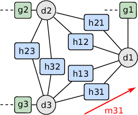
The gnn that is complementary to one time step of the cl factor graph is shown in Fig. 1(b). Since the cl factor graph only consists of pairwise interactions, we can use a simpler gnn compared to the one originally proposed for nebp [15], i.e. a gnn that only models variables nodes in the factor graph by a corresponding gnn node. In what follows, we denote the nebp messages and their joint vector by $\underline{\bm{\mathbf{\phi}}}^{(t)}$ and $\underline{\bm{\mathbf{\phi}}}_{j\rightarrow i}^{(t)}$, respectively.

nebp for cl consists of the following three

steps:

1. 1.

   First, classical bp runs for one iteration,

   i.e.,

   $\displaystyle\bm{\mathbf{\phi}}^{(t)}$

   $\displaystyle=\text{BP}\big(\underline{\bm{\mathbf{\phi}}}^{(t-1)}\hskip-0.85358pt\hskip-0.85358pt,\bm{\mathbf{w}}\big).$

   (10)

   Here $\text{BP}(\cdot)$ is the function that

   takes nebp messages $\underline{\bm{\mathbf{\phi}}}^{(t-1)}$ and $\bm{\mathbf{w}}$ as

   inputs and returns the

   bp messages $\bm{\mathbf{\phi}}^{(t)}$ by

   first computing (7)

   (with $t$ replaced by $t\hskip-0.85358pt-\hskip-0.85358pt1$ and $\bm{\mathbf{\phi}}_{j\to i}^{(t,k)}$ replaced

   by $\underline{\bm{\mathbf{\phi}}}_{j\to i}^{(t-1,k)}$) followed by (6) for all edges $(j,i)$, $i\hskip-0.85358pt\in\hskip-0.85358pt{\cal{I}}$, $j\in{\cal{N}}_{i}$ in the network. At iteration $t\hskip-0.85358pt=\hskip-0.85358pt1$, $\underline{\bm{\mathbf{\phi}}}^{(t-1)}$ in

   (10) is replaced by

   the

   all-ones vector with dimension $K\hskip 0.85358pt\sum^{I}_{i=1}|{\cal{N}}_{i}|$.

2. 2.

   Next, the output of the GNN is

   computed,

   i.e.,

   $\displaystyle\big[\bm{\mathbf{h}}^{(t+1)\text{T}}\hskip 0.85358pt\hskip 0.85358pt\hskip 0.85358pt\bm{\mathbf{m}}^{(t)\text{T}}\big]^{\hskip-0.85358pt\text{T}}$

   $\displaystyle=\text{GNN}\big(\bm{\mathbf{h}}^{(t)}\hskip-0.85358pt\hskip-0.85358pt,\bm{\mathbf{\phi}}^{(t)}\big)$

   where $\text{GNN}(\cdot)$ is the function that calculates gnn messages $\bm{\mathbf{m}}^{(t)}$ and updated node embeddings $\bm{\mathbf{h}}^{(t+1)}\hskip-0.85358pt\hskip-0.85358pt$ from the current node embeddings $\bm{\mathbf{h}}^{(t)}$ and the classical bp messages $\bm{\mathbf{\phi}}^{(t)}\hskip-0.85358pt\hskip-0.85358pt$ using (8)–(9). In

   particular, the classical

   bp messages $\bm{\mathbf{\phi}}^{(t)}_{j\to i}$, $i\hskip-0.85358pt\in\hskip-0.85358pt{\cal{I}}$, $j\in{\cal{N}}_{i}$ are used as the edge attributes $\bm{\mathbf{a}}_{j\to i}$ in (8).

   At $t\hskip-0.85358pt=\hskip-0.85358pt1$, $\bm{\mathbf{h}}^{(1)}$ is initialized by setting $\bm{\mathbf{h}}_{i}^{(1)}\hskip-0.85358pt=\hskip-0.85358pt\big[\hat{\bm{\mathbf{x}}}_{i}^{\text{T}}\hskip 0.85358pt\hskip 0.85358pt\text{vec}(\hat{\bm{\mathbf{C}}}_{i})^{\text{T}}\big]^{\text{T}}$ for all $i\in{\cal{I}}$, where $\hat{\bm{\mathbf{x}}}_{i}\hskip-0.85358pt=\sum_{k=1}^{K}w_{i}^{(k)}\bm{\mathbf{x}}_{i}^{(k)}$ is the sample mean, $\hat{\bm{\mathbf{C}}}_{i}\hskip-0.85358pt=\sum_{k=1}^{K}w_{i}^{(k)}(\bm{\mathbf{x}}_{i}^{(k)}-\hat{\bm{\mathbf{x}}}_{i})(\bm{\mathbf{x}}_{i}^{(k)}-\hat{\bm{\mathbf{x}}}_{i})^{\text{T}}$ is the sample

   covariance, and $\text{vec}(\cdot)$ creates a vector from the input matrix by taken elements columnwise.

3. 3.

   Finally, for all edges $(j,i)$, $i\hskip-0.85358pt\in\hskip-0.85358pt{\cal{I}}$, $j\in{\cal{N}}_{i}$, gnn messages $\bm{\mathbf{m}}^{(t)}_{j\to i}$ and bp messages $\bm{\mathbf{\phi}}_{j\to i}^{(t)}$ are combined according to

   $\displaystyle\underline{\bm{\mathbf{\phi}}}_{j\to i}^{(t)}$

   $\displaystyle=g_{\mathrm{s}}(\bm{\mathbf{m}}_{j\to i}^{(t)})\hskip 0.85358pt\bm{\mathbf{\phi}}_{j\to i}^{(t)}+g_{\mathrm{v}}(\bm{\mathbf{m}}_{j\to i}^{(t)}).$

   The functions $g_{\mathrm{s}}(\cdot)$ and $g_{\mathrm{v}}(\cdot)$ are neural networks with learnable parameters and output a positive scalar and a positive vector, respectively.

After $T$ iterations, the particle representation $\{\bm{\mathbf{x}}_{i}^{(k)}\hskip-0.85358pt,\underline{w}_{i}^{(T,k)}\}_{k=1}^{K}$ of the nebp belief $\underline{b}_{i}^{(T)}(\bm{\mathbf{x}}_{i})$ is obtained by calculating weights $\underline{w}_{i}^{(T,k)}$ based on (7) with bp messages $\bm{\mathbf{\phi}}_{j\to i}^{(T,k)}$ replaced by nebp messages $\underline{\bm{\mathbf{\phi}}}_{j\to i}^{(T,k)}$. The particle representation $\{\bm{\mathbf{x}}_{i}^{(k)}\hskip-0.85358pt,\underline{w}_{i}^{(T,k)}\}_{k=1}^{K}$ can then be used to calculate an approximate MMSE estimate $\underline{\hat{\bm{\mathbf{x}}}}_{i}$ and the corresponding approximate covariance matrix. Since we aim to reduce the MSE of the position estimate $\underline{\hat{\bm{\mathbf{p}}}}_{i}$, the neural networks $g_{\mathrm{e}}(\cdot)$, $g_{\mathrm{n}}(\cdot)$, $g_{\mathrm{s}}(\cdot)$, and $g_{\mathrm{v}}(\cdot)$ are trained based on the loss function

$\sum^{I}_{i=1}\hskip-0.85358pt\|\underline{\hat{\bm{\mathbf{p}}}}_{i}-\bm{\mathbf{p}}_{i}\|^{2}\hskip-0.85358pt$.

We consider agent networks in 2d (2d) space. The state of each agent at time $n$ is defined as $\bm{\mathbf{x}}_{i,n}=[\bm{\mathbf{p}}_{i,n}^{\text{T}}\hskip 0.85358pt\bm{\mathbf{v}}_{i,n}^{\text{T}}]^{\text{T}}\in\mathbb{R}^{4}$ where $\bm{\mathbf{p}}_{i,n}\in\mathbb{R}^{2}$ and $\bm{\mathbf{v}}_{i,n}\in\mathbb{R}^{2}$ are the 2d position and velocity, respectively. We use a constant-velocity motion model with drag force and Gaussian driving noise with standard deviation $\sigma_{a}=0.05$ (see [22] for details). Furthermore, we consider measurements of the distance $z_{j\to i,n}=\|\bm{\mathbf{p}}_{j,n}-\bm{\mathbf{p}}_{i,n}\|+r_{j\to i,n}$, where $r_{j\to i,n}$ is zero-mean Gaussian noise with standard deviation $\sigma_{r}=1$.

We consider $I\hskip-0.85358pt=\hskip-0.85358pt25$ agents on the area of interest $[0,60]\text{m}\times[0,60]\text{m}$. There are five static anchors at perfectly known locations, i.e., their state transition model and prior distribution are given by $p(\bm{\mathbf{x}}_{i,n}|\bm{\mathbf{x}}_{i,n-1})\hskip-0.85358pt=\hskip-0.85358pt\delta(\bm{\mathbf{x}}_{i,n}-\bm{\mathbf{x}}_{i,n-1})$ and $p\big(\bm{\mathbf{x}}_{i,0})\hskip-0.85358pt=\delta(\bm{\mathbf{x}}_{i,0}$ $-[\overline{\bm{\mathbf{p}}}_{i}^{\text{T}}\hskip 0.85358pt\hskip 0.85358pt\hskip 0.85358pt0\hskip 0.85358pt\hskip 0.85358pt\hskip 0.85358pt0]^{\text{T}}\big)$ where $\overline{\bm{\mathbf{p}}}_{i}$ is the true anchor position. In each realization, the mobile agents are uniformly placed over the area $[15,45]\text{m}\times[15,45]\text{m}$ and their velocity is randomly drawn from ${\cal{N}}(\bm{\mathbf{0}},\sigma_{p}^{2}\bm{\mathbf{I}}_{2})$ with $\sigma_{p}=0.1$. For each agent, a track that consists of 50 time steps is generated and range measurements are obtained by assuming a connectivity of $20$m, i.e. $j\hskip-0.85358pt\in\hskip-0.85358pt{\cal{N}}_{i}$ if and only if $\|\bm{\mathbf{p}}_{j,n}-\bm{\mathbf{p}}_{i,n}\|\leq 20\text{m}$. For inference, the initial prior distribution is $p(\bm{\mathbf{x}}_{i,0})={\cal{N}}(\bm{\mathbf{\mu}}_{i,0},\bm{\mathbf{\Sigma}}_{i,0})$. Here $\bm{\mathbf{\Sigma}}_{i,0}=\text{diag}\{10,10,0.01,0.01\}$ and $\bm{\mathbf{\mu}}_{i,0}$ is randomly drawn from ${\cal{N}}(\bm{\mathbf{x}}_{i,0},\bm{\mathbf{\Sigma}}_{i,0})$, where $\bm{\mathbf{x}}_{i,0}$ is the true initial state of agent $i$.

References

- [1] Y. Bar-Shalom, X. R. Li, and T. Kirubarajan, Estimation with Applications to Tracking and Navigation. New York, NY: Wiley, 2001.
- [2] N. Patwari, J. N. Ash, S. Kyperountas, A. O. Hero, R. L. Moses, and N. S. Correal, “Locating the nodes: Cooperative localization in wireless sensor networks,” IEEE Signal Process. Mag., vol. 22, no. 4, pp. 54–69, Jul. 2005.
- [3] A. Bahr, M. R. Walter, and J. J. Leonard, “Consistent cooperative localization,” in Proc. IEEE ICRA-09, Kobe, Japan, 2009, pp. 3415–3422.
- [4] R. D. Taranto, S. Muppirisetty, R. Raulefs, D. T. Slock, T. Svensson, and H. Wymeersch, “Location-aware communications for 5G networks: How location information can improve scalability, latency, and robustness of 5G,” IEEE Signal Process. Mag., vol. 31, no. 6, pp. 102–112, Nov. 2014.
- [5] A. T. Ihler, J. W. Fisher III, R. L. Moses, and A. S. Willsky, “Nonparametric belief propagation for self-localization of sensor networks,” IEEE J. Sel. Areas Commun., vol. 23, no. 4, pp. 809–819, Apr. 2005.
- [6] H. Wymeersch, J. Lien, and M. Z. Win, “Cooperative localization in wireless networks,” Proc. IEEE, vol. 97, no. 2, pp. 427–450, 2009.
- [7] M. Z. Win, F. Meyer, Z. Liu, W. Dai, S. Bartoletti, and A. Conti, “Efficient multi-sensor localization for the Internet-of-Things,” IEEE Signal Process. Mag., vol. 35, no. 5, pp. 153–167, Sep. 2018.
- [8] F. Meyer, T. Kropfreiter, J. L. Williams, R. A. Lau, F. Hlawatsch, P. Braca, and M. Z. Win, “Message passing algorithms for scalable multitarget tracking,” Proc. IEEE, vol. 106, no. 2, pp. 221–259, Feb. 2018.
- [9] F. R. Kschischang, B. J. Frey, and H.-A. Loeliger, “Factor graphs and the sum-product algorithm,” IEEE Trans. Inf. Theory, vol. 47, no. 2, pp. 498–519, Feb. 2001.
- [10] Y. Weiss and W. T. Freeman, “Correctness of belief propagation in Gaussian graphical models of arbitrary topology,” Neural Comput., vol. 13, no. 10, pp. 2173–2200, 2001.
- [11] B. Li and Y.-C. Wu, “Convergence of Gaussian belief propagation under general pairwise factorization: Connecting Gaussian MRF with pairwise linear Gaussian model.” JMLR, vol. 20, no. 144, pp. 1–30, 2019.
- [12] M. Gori, G. Monfardini, and F. Scarselli, “A new model for learning in graph domains,” in Proc. INNS/IEEE IJCNN-05, vol. 2, Montreal, Canada, 2005, pp. 729–734.
- [13] F. Scarselli, M. Gori, A. C. Tsoi, M. Hagenbuchner, and G. Monfardini, “The graph neural network model,” IEEE Trans. Neural Netw., vol. 20, no. 1, pp. 61–80, 2009.
- [14] K. Yoon, R. Liao, Y. Xiong, L. Zhang, E. Fetaya, R. Urtasun, R. Zemel, and X. Pitkow, “Inference in probabilistic graphical models by graph neural networks,” in Proc. IEEE Asilomar-19, Pacific Grove, CA, 2019, pp. 868–875.
- [15] V. G. Satorras and M. Welling, “Neural enhanced belief propagation on factor graphs,” in Proc. AISTATS-21, Apr. 2021, pp. 685–693.
- [16] F. Meyer, O. Hlinka, and F. Hlawatsch, “Sigma point belief propagation,” IEEE Signal Process. Lett., vol. 21, no. 2, pp. 145–149, Feb. 2014.
- [17] F. Meyer, O. Hlinka, H. Wymeersch, E. Riegler, and F. Hlawatsch, “Distributed localization and tracking of mobile networks including noncooperative objects,” IEEE Trans. Signal and Inf. Process. over Networks, vol. 2, no. 1, pp. 57–71, 2016.
- [18] F. Meyer, H. Wymeersch, M. Fröhle, and F. Hlawatsch, “Distributed estimation with information-seeking control in agent networks,” IEEE J. Sel. Areas Commun., vol. 33, no. 11, Nov. 2015.
- [19] J. Gilmer, S. S. Schoenholz, P. F. Riley, O. Vinyals, and G. E. Dahl, “Neural message passing for quantum chemistry,” in Proc. ICML-17, Sydney, Australia, Aug. 2017, pp. 1263–1272.
- [20] T. N. Kipf and M. Welling, “Semi-supervised classification with graph convolutional networks,” in Proc. ICLR-17, Toulon, France, Apr. 2017.
- [21] I. Goodfellow, Y. Bengio, and A. Courville, Deep Learning. Cambridge, MA: MIT Press, 2016.
- [22] S. Van de Velde, G. T. de Abreu, and H. Steendam, “Improved censoring and NLOS avoidance for wireless localization in dense networks,” IEEE J. Sel. Areas Commun., vol. 33, no. 11, pp. 2302–2312, 2015.
- [23] D. P. Kingma and J. Ba, “Adam: A method for stochastic optimization,” arXiv preprint arXiv:1412.6980, 2014.