Estimating the variance of Shannon entropy

The system of interest consists of $M$ states and has a purely stochastic evolution: the transition probability from state $j$ to state $i$ is independent of $j$, where, here and henceforth, both $i$, $j$ run between 1 and $M$. Let $s_{i}$ be the probability with which the $i$-th state is visited. The Shannon entropy $H$ of the system is given by

Throughout the paper it is assumed—via continuous extension—that ${x\ln^{n}x=0}$ if ${x=0}$, for each ${n\in\mathbb{N}}$. However, unless otherwise specified, we suppose here that $M$ coincides with the size of the support of the distribution ${\{s_{i}\}}$, so that ${s_{i}>0,\,\forall i}$.

A way to estimate $H$ relies on the plug-in estimator $\widehat{H}$, as follows. (Henceforth, given a typically unknown quantity $a$, the symbol $\widehat{a}$ refers to an estimator of $a$ that, as a function of observed data, is a statistic affected by bias and fluctuations). We consider $N$ consecutive steps of the system’s evolution and record the $M$-dimensional set ${\{\widehat{j}_{i}\}}$ of the number of visits of each one of the $M$ states. The set ${\{\widehat{j}_{i}\}}$ is distributed according to a multinomial distribution, and it holds that ${\sum_{i=1}^{M}\widehat{j}_{i}=N}$. Upon computing, for each $i$, the observed rate $\widehat{p}_{i}$ as ${\widehat{p}_{i}=\widehat{j}_{i}/N}$, the plug-in estimator $\widehat{H}$ is defined as

The plug-in estimator is affected by a bias term that is known as the Miller-Madow correction Miller 1955; Basharin 1959; Harris 1975 and is equal to ${-(M-1)/(2N)}$. With regard to the variance of the plug-in estimator, let first the variance parameter $\Lambda_{0}$ be defined as

Then, as shown by Basharin Basharin 1959 and Harris Harris 1975, in the multinomial case and provided that ${\Lambda_{0}>0}$, the variance $\sigma^{2}_{\widehat{H}}$ is given by

Noteworthily, by writing $\Lambda_{0}$ in the form mentioned in Sec. I, namely ${\Lambda_{0}=\sum_{i=1}^{M}s_{i}\left(H+\ln s_{i}\right)^{2}}$, it can be promptly shown that ${\Lambda_{0}\geqslant 0}$, where the equality holds if and only if the probabilities $s_{i}$ are uniformly distributed.

As pointed out in the Introduction, estimating the variance of the plug-in estimator requires the knowledge of the parameter $\Lambda_{0}$, for which an estimator is proposed and analyzed in the following sections.

The estimator of the variance parameter $\Lambda_{0}$ proposed in this paper is the plug-in estimator that is evaluated out of the rate histogram ${\{\widehat{p}_{i}\}}$ as

Because the quantity $\widehat{\Lambda_{0}}$ is a sample statistic, it is necessary to assess its reliability in terms of bias and variance. This issue is tackled by determining the asymptotic behavior of $\widehat{\Lambda_{0}}$ as ${N\to\infty}$. To this goal, it is suitable to define, for each $i$, ${\zeta_{i}\equiv\left(\widehat{p}_{i}-s_{i}\right)\sqrt{N}}$, so that the rates can be expressed as

It follows:

Expanding the previous expression in terms of order $N^{-n/2}$, with ${n\in\mathbb{N}}$, leads to

where ${\ell_{i}\equiv\ln s_{i}}$ and the identity ${\sum_{i=1}^{M}\zeta_{i}=0}$, which follows from the constraint ${\sum_{i=1}^{M}\widehat{p}_{i}=1}$, was used.

Let ${G_{\delta\widehat{\Lambda_{0}}}(t)}$ be the moment generating function of the residual ${\delta\widehat{\Lambda_{0}}\equiv\widehat{\Lambda_{0}}-\Lambda_{0}}$, where $t$ is a real variable defined in a neighborhood of the origin. It holds that

The exponential form ${e^{t\,\delta\widehat{\Lambda_{0}}}}$ can be expressed as

Because the starting vector of the system’s evolution is randomly chosen according to the distribution ${\{s_{i}\}}$, the expected value of each $\zeta_{i}$ is given by Ricci 2021a ${\E\left(\zeta_{i}\right)=O\left(1/N\right)}$, so that the term proportional to ${t/\sqrt{N}}$ is absorbed within the term ${O\left(N^{-3/2}\right)}$. In addition Ricci 2021a, one has ${\E\left(\zeta_{i}\zeta_{j}\right)=\chi_{i,j}+O\left(N^{-1/2}\right)}$, where ${\chi_{i,j}=\delta_{i,j}s_{i}-s_{i}s_{j}}$ is the covariance matrix of rates being distributed according to a multinomial distribution ($\delta_{i,j}$ is the Kronecker delta). It follows:

Let the coefficients of ${t/N}$ and ${t^{2}/(2N)}$ in Eq. (4) be defined as $\gamma$ and $\Gamma$, respectively:

Equation (4) can be then rewritten as:

It is worth noting that, because $\chi$ is positive semi-definite, from the definition of $\Gamma$ one has ${\Gamma\geqslant 0}$.

As a consequence of the properties of the moment generating function, the coefficient of $t$ in this last equation corresponds to the expected value of $\delta\widehat{\Lambda_{0}}$, i.e. of ${\widehat{\Lambda_{0}}-\Lambda_{0}}$:

Also, because the square of this last term is of order $N^{-2}$, the coefficient of $t^{2}/2$ in Eq. (5) directly provides the variance of $\delta\widehat{\Lambda_{0}}$ and thus of $\widehat{\Lambda_{0}}$:

Equations (6), (7) provide the bias and the variance of the plug-in estimator $\widehat{\Lambda_{0}}$ of the variance parameter $\Lambda_{0}$, respectively.

Besides these results, Eq. (5) can be further exploited: starting from it, the moment generating function of the random variable ${w\equiv\left(\delta\widehat{\Lambda_{0}}-\frac{\gamma}{N}\right)\sqrt{N}}$ is given by:

where $t$ is a real variable defined in a neighborhood of the origin. This expression shows that, provided that ${\Gamma}$ is non-vanishing, $w$ is asymptotically normally distributed with zero mean and variance ${\Gamma}$. It is therefore possible to formulate a central limit theorem for the plug-in estimator $\widehat{\Lambda_{0}}$ of the variance parameter $\Lambda_{0}$:

The main result of this section can be summarized as the fact that the plug-in estimator $\widehat{\Lambda_{0}}$ defined in Eq. (3) is asymptotically normal and is a consistent estimator (both its population mean and variance depend on $N^{-1}$) of the variance parameter $\Lambda_{0}$.

From a practical point of view, using the asymptotic expressions above requires the knowledge of the parameters $\gamma$ and $\Gamma$. The two parameters can be expressed upon straightforward algebra as

where $\mu_{3}$, $\mu_{4}$ are the third and fourth moments of the distribution of the single-bin entropy ${-\ell_{i}=-\ln s_{i}}$, which are generally defined as

so that, for example, ${\mu_{1}^{\prime}=H}$, ${\mu_{2}^{\prime}=\Lambda_{0}+H^{2}}$.

The presence, in the expressions above, of ${\mu_{3}^{\prime}}$, ${\mu_{4}^{\prime}}$, ${\sum_{i}\ell_{i}}$, makes the estimates of $\gamma$, $\Gamma$, and thus of $\widehat{\Lambda_{0}}$, a circular problem. In principle, provided that sufficiently large data samples are available, one could carry out a statistical analysis on subsamples of different size $N$, in order to “experimentally assess” the parameters $\gamma$, $\Gamma$. In practice however, and especially in the case of limited data samples, it is difficult to estimate the reliability of $\widehat{\Lambda_{0}}$ and thus of the variance of the estimated Shannon entropy $\widehat{H}$. In the next section this issue is circumvented by evaluating the maximum value of $\Lambda_{0}$ as a function of the number $M$ of the system’s states.

Because the probabilities $s_{i}$ have to add up to one, only ${M-1}$ values are independent. We then consider $s_{M}$ as a function of the other $M-1$ probabilities:

To find the stationary points of $\Lambda_{0}$, its partial derivative with respect to the independent $s_{i}$’s, with ${1\leqslant i\leqslant M-1}$, is considered:

A vanishing partial derivative requires fulfilling one of two possibilities, namely

The two possibilities are mutually-excluding: if it were ${p_{0}=q_{0}}$, then it would follow, first, ${s_{i}=1/M}$, ${\forall i\in[1,\,M]}$, so that ${H=\ln M}$, and, second, ${s_{M}=\frac{1}{s_{M}}e^{-2-2H}}$, so that ${H=1+\ln M}$. Therefore it must hold that ${p_{0}\neq q_{0}}$.

Let $k$ be the number of $s_{i}$’s that satisfy the first possibility, Eq. (11). Because $s_{M}$ trivially satisfies this condition, one has ${1\leqslant k\leqslant M}$. However, the case ${k=M}$ corresponds to a uniform distribution where ${s_{i}=1/M}$, ${\forall i\in[1,\,M]}$. In this case, ${\Lambda_{0}=0}$ and, as shown by Harris Harris 1975, the dominant variance term is of order $N^{-2}$. The uniform distribution thus yields the vanishing, minimum value of $\Lambda_{0}$, which also occurs in the $M$ vertices of the simplex, namely whenever a single $s_{i}$ is unitary while all the others are vanishing. Henceforth we therefore restrict the discussion to the range ${1\leqslant k\leqslant M-1}$. The number of $s_{i}$’s that satisfy the second possibility, Eq. (12), is then ${M-k}$, which also varies between 1 and ${M-1}$.

Equations (1), (10), (12) can be respectively rewritten as follows:

Equations (13), (14), (15) make up a system of three equations in the three variables $H$, $p_{0}$, $q_{0}$, while the integer number $k$ is a fixed parameter. Inserting the expression for $H$ given by Eq. (13) into Eq. (15) and replacing $q_{0}$ with ${\frac{1-kp_{0}}{M-k}}$, as given by Eq. (14), yields:

Crucially, because of Eq. (14) and the fact that we are considering the interior of $\mathbb{D}$, it holds that ${0<kp_{0}<1}$ and ${0<(M-k)q_{0}<1}$.

It is useful to introduce the auxiliary variable $v$ defined as

It follows:

By also defining the function $f(v)$ as

Eq. (16) can be rewritten as

The graph of $f(v)$ corresponds to the continuous, red line shown in Fig. 1.

It is straightforward to show that ${f(v)}$ satisfies the following properties: ${f(-v)=f(v)}$; ${f(v)\geqslant 0}$; ${f(v)\to+\infty}$ as ${v\to\pm 1}$. In addition, because the derivative ${f^{\prime}(v)}$ is given by

the function ${f(v)}$ is monotonically increasing (decreasing) if ${v>0}$ (${v<0}$) and thus has a single minimum equal to 0 in ${v=0}$. As it is also shown in Fig. 1, the right-hand term of Eq. (20) is instead a straight-line going through the point ${(0,2)}$ and having a slope ${-\ln\frac{M-k}{k}}$.

For any $k$, the roots of the transcendental Eq. (20) provide, via Eqs. (17), (18), stationary points for ${\Lambda_{0}=\Lambda_{0}(p_{0},p_{1},\dots,p_{M-1})}$. Let $\tilde{v}_{k}$ be a root of Eq. (20) for a given $k$. According to Eq. (2) and by using Eq. (17), (18), the variance parameter $\Lambda_{0}$ can be promptly rewritten as

It then follows that the maximum value of $\Lambda_{0}$ occurs for a stationary point characterized by a value $k$ that yields the minimum $|\tilde{v}_{k}|$.

To assess this $k$ value and the corresponding minimum $|\tilde{v}_{k}|$ we start observing that for each $k$ there are two roots of Eq. (20), one negative and one positive, which are henceforth referred to as $-\tilde{v}_{k,1}$, $\tilde{v}_{k,2}$, respectively, with ${\tilde{v}_{k,1}>0}$, ${\tilde{v}_{k,2}>0}$. From Eq. (20) it holds that ${\tilde{v}_{M-k,2}=\tilde{v}_{k,1}}$. It is therefore sufficient to study the cases ${k\leqslant M/2}$ for which the factor ${\ln\frac{M-k}{k}}$ is non-negative.

Inserting ${-\tilde{v}_{k,1}}$, ${\tilde{v}_{k,2}}$ in Eq. (20) and subtracting the results yields

Consequently, ${f\left(\tilde{v}_{k,1}\right)=f\left(-\tilde{v}_{k,1}\right)\geqslant f\left(\tilde{v}_{k,2}\right)}$ and, because $f(v)$ is monotonically increasing if ${v>0}$, it follows ${\tilde{v}_{k,1}\geqslant\tilde{v}_{k,2}}$. The root $\tilde{v}_{k,2}$ is therefore the closest one to the origin.

We now show that $\tilde{v}_{k,2}$ decreases if $k$ increases by one. Because ${\frac{M-k}{k}>\frac{M-k-1}{k+1}}$, one has

i.e.

If it were ${\tilde{v}_{k,2}\geqslant\tilde{v}_{k+1,2}}$, the left-hand term of the previous inequality would be non-positive, whereas the right-hand term would be non-negative (the function ${f(v)/v=\ln\frac{1+v}{1-v}}$ is monotonically increasing if ${0<v<1}$), thus leading to a contradiction. It then must hold that ${\tilde{v}_{k,2}<\tilde{v}_{k+1,2}}$. Consequently, $\tilde{v}_{1,2}$ provides the minimum absolute value of a root of Eq. (20) and thus, via Eq. (21), the maximum value of $\Lambda_{0}$ for a given $M$ with regard to the interior of the simplex $\mathbb{D}$.

As a corollary, the very same argument of the last paragraph can be promptly applied to show that increasing $M$ leads to a decrease of $\tilde{v}_{1,2}$ and thus to an increase of $\Lambda_{0,\,\text{max}}$. This corollary is important in order to discuss the behavior of the variance parameter $\Lambda_{0}$ on the boundary of the probability simplex.

It is finally important to note that, when ${k=1}$, the single outlier among the set of probabilities ${\{s_{i}\}}$ is $s_{M}$, namely the one that was chosen as dependent on all the others [see Eq. (10)]. Because $M$ similar choices are possible, the number of equivalent maxima of $\Lambda_{0}$ is $M$.

The boundary ${\partial\mathbb{D}}$ of the $M$-simplex $\mathbb{D}$ is the union of $M$ boundary facets. Each facet is defined by a single $s_{j}$, with ${1\leqslant j\leqslant M}$, set to zero, and it thus corresponds to a ${(M-1)}$-simplex.

This last assumption contradicts the fact that $M$ is the support size of the probability distribution. However, we discuss these cases for the sake of completeness and because, in principle, one could have arbitrarily small $s_{i}$ values.

Because each facet corresponds to a simplex, the arguments of the previous section can be iteratively applied as follows. First, in the interior of the $j$-th facet, the maximum of $\Lambda_{0}$ will be ${1/\tilde{v^{\prime}}_{1,2}^{2}-1}$, where $\tilde{v^{\prime}}_{1,2}$ is the negative root of Eq. (20) when ${k=1}$ and $M$ is replaced by ${M-1}$. Second, the boundary of the $j$-th facet has to be treated as a ${(M-2)}$-dimensional set of ${(M-2)}$-simplexes, and so on. The iteration stops at the two-dimensional simplexes in which only a pair ${(s_{i},\,s_{j})}$ of probabilities is nonzero: in this case the boundaries are the point-like vertices of a segment, in which ${\Lambda_{0}=0}$.

Because of the corollary expressed at the end of the previous section, Sec. III.1, the maximum of $\Lambda_{0}$ on the $j$-th facet is strictly less than the value produced by a stationary point lying within $\mathbb{D}$, namely ${1/\tilde{v}_{1,2}^{2}-1}$.

By taking into account the results of Sections III.1, III.2, we can conclude that the maximum of $\Lambda_{0}$ in the multinomial case occurs when the distribution of the probabilities ${\{s_{i}\,|\,i\in[1,\,M]\}}$ has a single entry equal to the value $p_{0}$ and all the other entries uniformly distributed and equal to $q_{0}$.

Upon finding the single positive root ${\tilde{v}\equiv\tilde{v}_{1,2}}$ of the transcendental equation

which corresponds to Eq. (20) with ${k=1}$, one has

Equation (22) can be approximately solved by replacing $f(v)$ with the first term of its Taylor expansion, namely $2v^{2}$. Equation (22) then becomes a second-degree equation whose positive solution is given by

which, for large $M$ values, can be further approximated as ${\tilde{v}\sim 2/\ln(M)}$. (These approximations improve with $M$ because the larger $M$, the smaller $\tilde{v}$). Figure 2 shows the plots of $p_{0}$, $\Lambda_{0,\,\text{max}}$ as a function of the dimension $M$. The approximation based on Eq. (25) works well for ${M\gtrsim 10}$.

It is worth observing that, as ${M\to\infty}$, one has

while $p_{0}$ tends to 1/2.

The number of different distributions that maximize $\Lambda_{0}$ is equal to $M$, one for each state taking on the value $p_{0}$. Figure 3 shows the case ${M=3}$.

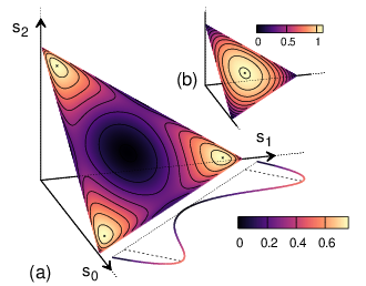
It is important to note that, in the case of a distribution that maximizes $\Lambda_{0}$, the parameter $\Gamma$, which is given by Eq. (9) and describes the $N^{-1}$ dependence of the plug-in estimator $\widehat{\Lambda_{0}}$ of $\Lambda_{0}$, vanishes. A proof of this statement is discussed in the appendix. The situation is similar to what happens to the plug-in entropy estimator $\widehat{H}$ when the distribution is uniform: in this case $H$ takes on its maximum value equal to ${\ln(M)}$, while the quantity that describes the expected value of the variance of the plug-in estimator, namely $\Lambda_{0}/N$, vanishes and it is replaced by higher-order terms (typically ${\sim N^{-2}}$ Harris 1975). The same is expected to occur in the case of $\Gamma$.

Finally, it is worth considering how “peaked” the maxima of $\Lambda_{0}$ are. The partial derivatives with respect to the independent $s_{i}$’s, evaluated in the locations corresponding to ${\Lambda_{0}=\Lambda_{0,\,\text{max}}}$ are given by

where the last approximation holds provided that ${M\gg 1}$ so that ${\tilde{v}\sim 2/\ln(M)}$. In this limit, upon defining $\delta s_{M}$ and $\delta s_{\parallel}$ as

where $\delta s_{i}$ is the infinitesimal displacement of the respective $s_{i}$ from the value $q_{0}$, we have the following Taylor expansion for $\Lambda_{0}$:

References

- Shannon (1948) C. E. Shannon, Bell Syst. Techn. J. 27, 379 (1948).
- Cover and Thomas (2006) T. M. Cover and J. A. Thomas, Elements of Information Theory, 2nd ed. (John Wiley & Sons, Hoboken, New Jersey, 2006).
- Bandt and Pompe (2002) C. Bandt and B. Pompe, Phys. Rev. Lett. 88, 174102 (2002).
- Delgado-Bonal and Marshak (2019) A. Delgado-Bonal and A. Marshak, Entropy 21, 541 (2019).
- Strong et al. (1998) S. P. Strong, R. Koberle, R. R. de Ruyter van Steveninck, and W. Bialek, Phys. Rev. Lett. 80, 197 (1998).
- Dimitrov et al. (2011) A. G. Dimitrov, A. A. Lazar, and J. D. Victor, J. Comput. Neurosci. 30, 1 (2011).
- Sayood (2018) K. Sayood, Entropy 20, 706 (2018).
- Vinga (2014) S. Vinga, Brief. Bioinform. 15, 376 (2014).
- Koonin (2016) E. V. Koonin, Philos. T. R. Soc. A 374, 20150065 (2016).
- Chanda et al. (2020) P. Chanda, E. Costa, J. Hu, S. Sukumar, J. Van Hemert, and R. Walia, Entropy 22, 627 (2020).
- Burggren and Monticino (2005) W. W. Burggren and M. G. Monticino, J. Exp. Biol. 208, 3221 (2005).
- Darbellay and Wuertz (2000) G. A. Darbellay and D. Wuertz, Physica A 287, 429 (2000).
- Zapart (2009) C. A. Zapart, Physica A 388, 1157 (2009).
- Leung and North (1990) L. Leung and G. R. North, J. Climate 3, 5 (1990).
- Majda and Gershgorin (2010) A. J. Majda and B. Gershgorin, P. Natl. Acad. Sci. USA 107, 14958 (2010).
- Balasis et al. (2013) G. Balasis, R. V. Donner, S. M. Potirakis, J. Runge, C. Papadimitriou, I. A. Daglis, K. Eftaxias, and J. Kurths, Entropy 15, 4844 (2013).
- Wellmann (2013) J. F. Wellmann, Entropy 15, 1464 (2013).
- Perdigão et al. (2020) R. A. P. Perdigão, U. Ehret, K. H. Knuth, and J. Wang, Water Resour. Res. 56, e2019WR025270 (2020).
- Grassberger (1988) P. Grassberger, Phys. Lett. A 128, 369 (1988).
- Pardo (1995) J. A. Pardo, Appl. Math. Comput. 72, 33 (1995).
- Lesne et al. (2009) A. Lesne, J.-L. Blanc, and L. Pezard, Phys. Rev. E 79, 046208 (2009).
- Paninski (2003) L. Paninski, Neural Comput. 15, 1191 (2003).
- Antos and Kontoyiannis (2001) A. Antos and I. Kontoyiannis, Random Struct. Algor. 19, 163 (2001).
- Basharin (1959) G. P. Basharin, Theor. Probab. Appl. 4, 333 (1959).
- Miller (1955) G. Miller, “Note on the bias of information estimates,” in Information theory in Psychology II-B (Free Press, Glencoe, IL, 1955) pp. 95–100.
- Harris (1975) B. Harris, “The statistical estimation of entropy in the non-parametric case,” in Topics in Information Theory (North-Holland, Amsterdam, 1975) pp. 323–355.
- Vinck et al. (2012) M. Vinck, F. P. Battaglia, V. B. Balakirsky, A. J. H. Vinck, and C. M. A. Pennartz, Phys. Rev. E 85, 051139 (2012).
- Roulston (1999) M. S. Roulston, Physica D 125, 285 (1999).
- Kugiumtzis (2013) D. Kugiumtzis, Eur. Phys. J.-Spec. Top. 222, 401 (2013).
- Ricci (2021a) L. Ricci, Phys. Rev. E 103, 022215 (2021a).
- Courant and Hilbert (1953) R. Courant and D. Hilbert, Methods of Mathematical Physics, vol. I (Interscience Publishers, Inc., New York, 1953).
- Adams and Essex (1953) R. A. Adams and C. Essex, Calculus: a complete course. 7th ed. (Pearson Canada, Toronto, 1953).
- Ricci (2021b) L. Ricci, Chaos Soliton. Fract. 142, 110450 (2021b).