Finite sample guarantees for quantile estimation: An application to detector threshold tuning

The problem of anomaly detection occurs in many different fields. For example, in healthcare when devices monitor a patient or in governmental agencies to detect tax fraud. In this work, we look at anomaly detection in the context of a control system, where the feedback system is equipped with an anomaly detector on the controller side (see Fig. 1). The input to the anomaly detector can depend both on the measurements received as well as the actuator signals determined by the controller, which are not necessarily scalar variables. For example, if a Kalman filter is used the input to the anomaly detector are the actuator signals and the sensor measurements, which are used to determine the difference, $r$, between the received and predicted measurements. This difference can be further processed to determine the output $y_{D}$, e.g., $y_{D}=r^{\top}r$.

In the control system example, a small detector output $y_{D}\in\mathbb{R}$ typically indicates that the system works as predicted, while large outputs indicate an unpredicted behavior. However, in other applications, the detector output can also be a similarity measure, where a small value for $y_{D}$ indicates anomalous behavior (see, for example, [16]). In this work, we use the interpretation that a large output indicates anomalous behavior. Therefore, an alarm is triggered when $y_{D}$ exceeds a threshold $J_{D}\in\mathbb{R}$, i.e., $y_{D}>J_{D}$, and no alarm is triggered when $y_{D}\leq J_{D}$. Due to random processes, such as measurement noise, the detector output is also of a stochastic nature.

For the sake of simplicity, we assume a continuous CDF for the detector output. In an industrial process control context, the process is often controlled around a desired steady-state value, which can be seen as stationary. Hence, assuming that the detector output is a random variable with a constant distribution is a reasonable choice. Furthermore, if the plant has linear dynamics and the noise processes are Gaussian, a Kalman filter converges to a stationary distribution for its residual signals, which are often used as the input of the anomaly detector. If the anomaly detector has no internal dynamics, such as a neural network or norm-based detector, then the output of the detector is also a random variable with a fixed distribution.

The stochasticity of $y_{D}$ leads to alarms in the nominal case, so called false alarms, where the rate of false alarms depends on the threshold. Since false alarms incur unnecessary costs and too many false alarms make a detector unreliable, we can choose a large threshold to avoid too many false alarms. However, a too large threshold leads usually to a smaller detection rate of anomalies. Hence, there is a trade-off between the detection rate of anomalies and the false alarm rate in the nominal case when tuning the threshold. Furthermore, Urbina et al. [5] point out that there is also a trade-off between the impact an attacker that wants to keep $y_{D}$ below the threshold can have and the false alarm rate when choosing the detector threshold.

In addition to that, the nature of anomalies is in most cases unknown. Take, for example, a complex large-scale system such as the power grid, where many different types of anomalies, such as sensor and generator failures or attacks, can occur. Therefore, we often do not know which anomalies will occur and what detection rate we will obtain for a certain threshold $J_{D}$. Since it is simpler to focus only on the nominal case instead of trying to consider all possible anomalous behaviors, we will focus on finding a threshold that guarantees an acceptable false alarm rate. More specifically, we want to find the smallest threshold $J_{D}$ such that

holds, where $\gamma\in(0,1)$. The threshold $J_{D}$ will result in a false alarm probability of at most $1-\gamma$. We want to find the smallest threshold, because a trivial solution to guaranteeing an acceptable false alarm rate is to choose an arbitrarily large threshold, which in turn will also reduce the detection rate of anomalies.

In special cases, a closed form solution for the threshold exists, see, for example, [13], or the detector threshold can be approximated in a distributionally robust fashion, see [14]. If the output of the detector depends on the threshold as well, such as for the CUSUM and MEWMA detector with resetting, it is more difficult to determine a threshold that guarantees a desired false alarm rate. Detectors whose output depends on the threshold are one avenue of future work and will not be considered in this work.

Before we formulate the problem we consider, we want to define the notion of a $\gamma$-quantile.

Note that $J_{D}$ in Definition 1 is unique and finite because of the infimum operator and the fact that $\gamma\in(0,1)$. Since $F(J_{D})=\mathrm{prob}\{y_{D}\leq J_{D}\}$, we can immediately see that the threshold we are looking for in (1) is equivalent to the $\gamma$-quantile of the detector output distribution. Further, $\gamma$-quantiles can be obtained as optimizers of convex optimization problems (see [17]), which theoretically makes them efficient to calculate. However, it is often not possible to find an expression for the probability distribution of the detector output. A reason for that is that either the plant dynamics, the controller dynamics, the detector dynamics or all of them are highly nonlinear, such that the distribution of $y_{D}$ does not have a closed-form solution. Samples from the monitored process under nominal conditions are usually available, such that we can obtain samples from the detector output under nominal conditions. Due to the equivalence with $\gamma$-quantiles, we use sample-based quantile estimators for a sample-based estimate $\tilde{J}_{D}$ of the threshold $J_{D}$. In this work, we use $N$ independent and identically distributed (i.i.d.) samples of $y_{D}$, $\{y_{D,i}\}_{i=1}^{N}$, to estimate the detector threshold as

where $\beta\in(0,1)$. Note that (2) has the form of common quantile estimators used in software packages [8]. In our previous work, we showed how the quantile estimators can be derived from a sample approximation of the conditional Value-at-Risk [9].

Although the true threshold $J_{D}$ can be approximated via (2), an open problem is to determine how many samples we need to get a good approximation. A good approximation is often characterized by assuming that $|J_{D}-\tilde{J}_{D}|$ is small with high probability. Distribution-free bounds on the bias of quantile estimates can be found in [18], where these bounds are always fulfilled and not only with high probability. However, depending on the shape of the probability distribution even small changes from the the threshold $J_{D}$ can lead to large deviations in the false alarm rate. Therefore, we are more interested in how close the false alarm rate $1-F(\tilde{J}_{D})$ is to the acceptable false alarm rate $1-F(J_{D})=1-\gamma$, since the acceptable false alarm rate is an important variable for the system operator.

Enforcing that the false alarm rate is close to the acceptable false alarm rate with a high probability, which means that $\epsilon$ and $\rho$ are close to zero, will intuitively lead to threshold estimates that are not just trivially large to guarantee the acceptable false alarm rate.

The first sample guarantee is based on the DKW inequality [10], which gives us probabilistic bounds on how close the empirical distribution function $F_{N}(y_{D})=\frac{1}{N}\sum_{i=1}^{N}\mathbf{1}_{\{y_{D,i}\leq y_{D}\}}$ is to the true cumulative distribution function $F(y_{D})$,

While the DKW inequality gives us bounds for the whole CDF, we will evaluate it only at the point of interest, which is $y_{D}=\tilde{J}_{D}$, to obtain our finite guarantees. Note that the result was presented in our previous paper [9], but is restated for the sake of completeness.

Instead of focusing on the whole probability distribution as in the previous section, we now use the statistics of order statistics to determine a finite sample guarantee which utilizes the Vysochanskij-Petunin inequality [11]. The Vysochanskij-Petunin inequality is given by

if $3\epsilon^{2}\geq 8\mathrm{Var}\{X\}$, where $X$ is a unimodal random variable with a finite mean and variance. Since for the Vysochanskij-Petunin inequality the expected value and variance of a random variable are needed, we introduce the expected value and variance of the CDF of a random variable evaluated at the $m$th order statistic.

In the previous section, we determined finite guarantees based on the Vysochanskij-Petunin inequality, which uses the expected value and variance of $F(y_{D,(m)})$. In this section, we will use that $F(y_{D,(m)})$ has a beta distribution and determine sample guarantees based on confidence intervals of the beta distribution. We begin by introducing a result on the confidence interval of a beta distributed random variable.

In this section we will discuss the three finite sample guarantees obtained previously, investigate their scaling in the parameters $\epsilon$ and $\rho$, and compare the sample sizes. For a given $\gamma$, $\epsilon$, and $\rho$, let $N_{\mathrm{DKW}}$, $N_{\mathrm{VP}}$, and $N_{\mathrm{beta}}$ be the sample sizes obtained from Proposition 1, Theorem 1, and Theorem 2, respectively. First, we want to discuss how to choose $\epsilon$. A reasonable bound for $\epsilon$ is $\epsilon\leq\min(\gamma,1-\gamma)$, because this choice results in $[\gamma-\epsilon,\gamma+\epsilon]\subseteq[0,1]$. This means that the $\pm\epsilon$-band around the acceptable false alarm rate contains only reasonable false alarm rates, i.e., false alarm rates in $[0,1]$. Further, with that choice we have $\frac{4}{9}\gamma(1-\gamma)\geq\frac{4}{9}\min(\gamma,1-\gamma)^{2}\geq\frac{4}{9}\epsilon^{2}>\frac{1}{6}\epsilon^{2}\geq\rho\epsilon^{2}$ if $\rho\leq\frac{1}{6}$. Hence, if $\rho\leq\frac{1}{6}$ the condition on both $\rho$ and $\epsilon$ in Theorem 1 is fulfilled for this bound of $\epsilon$.

Next, we want to investigate the scaling of each guarantee in the parameters $\epsilon$ and $\rho$. All finite guarantees scale with $\epsilon^{-2}$, while they differ in their scaling in $\rho$. The guarantee scales with $\ln(\rho^{-1})$, $\rho^{-1}$ and $z_{\frac{\rho}{2}}$ when it is obtained from Proposition 1, Theorem 1, and Theorem 2, respectively. Typically, we desire high probability guarantees such that $\rho$ is close to zero. It follows that Theorem 2 has the best scaling for $\rho\in(0,0.5]$ since then $z_{\frac{\rho}{2}}<\ln(\rho^{-1})<\rho^{-1}$.

Now, we compare the sample sizes from the three different finite guarantees when $\rho=0.05$ and $\epsilon=0.01$ for $\gamma\in[0.01,0.99]$. Fig. 2 shows the results of the comparison.

We see that the required sample size obtained from the DKW inequality is almost constant for different $\gamma$. This is expected because the DKW inequality applies for the whole cumulative distribution function. Further, we observe that Theorem 2 produces the smallest sample sizes out of the three finite guarantees for all investigated $\gamma$. We also observe that $N_{\mathrm{VP}}\leq N_{\mathrm{DKW}}$ if $\gamma\not\in(0.294,0.706)$. So only for $\gamma$ close to $0$ and $1$ the finite guarantees from Theorem 1 perform better than the finite guarantees from Proposition 1.

Both Fig. 2 and the scaling in $\rho$ and $\epsilon$ show us that the sample sizes we obtain from Theorem 2 are smaller than the sample sizes from Proposition 1 and Theorem 1 for all investigated $\gamma$. Furthermore, according to [12], the confidence bounds $\epsilon_{u}$ and $\epsilon_{l}$ are (nearly) exact if $N\geq 40$, since the influence of the higher order terms disappears.

We begin by evaluating the finite sample guarantees. The idea is to approximate the threshold of the anomaly detector with (2) based on $N$ samples, $\{y_{D,i}\}_{i=1}^{N}$, of the detector output and we do this approximation $N_{T}=1000$ times to obtain $N_{T}$ different approximations $\tilde{J}_{D}$ of $J_{D}$. Then we draw $10^{6}$ new samples of the detector output and calculate the empirical false alarm rate of each threshold.

Here, we investigate three different cases. First, we assume that the detector output has a $\chi^{2}(4)$ distribution, where we have four degrees of freedom. The samples are then taken i.i.d. from a $\chi^{2}(4)$ distribution. Second, we assume that the detector output has a Lévy distribution and obtain i.i.d. samples for the output from a Lévy distribution. Third, we assume the samples are taken from the trajectory of a non-parametric CUSUM detector [13] without resetting, given by

where $y_{D}(0)=0$, $\delta=6$, and $r(k)$ is the input of the detector and is drawn i.i.d. from a four-dimensional, zero-mean, multivariate Gaussian distribution at each time step $k$. Furthermore, we use $y_{D,i}=y_{D}(i)$ to obtain the samples, that is, the samples are the trajectory of the CUSUM detector. Therefore, the i.i.d. assumption on the samples is not fulfilled in this case.

For our simulation, we choose $\gamma=0.95$, $\epsilon=0.01$, and $\rho=0.05$, which means that the empirical false alarm rate should be in the interval $[0.04,0.06]$ with a probability of $95\,\%$. Moreover, Section III-D showed us that for these values of $\gamma$, $\epsilon$, and $\rho$, $N_{\mathrm{beta}}<N_{\mathrm{VP}}<N_{\mathrm{DKW}}$. Therefore, we investigate only the smallest and largest sample sizes, $N_{\mathrm{beta}}$ and $N_{\mathrm{DKW}}$, respectively, for the sake of clarity. In addition to that, we set $\beta=0$ when approximating the threshold with (2).

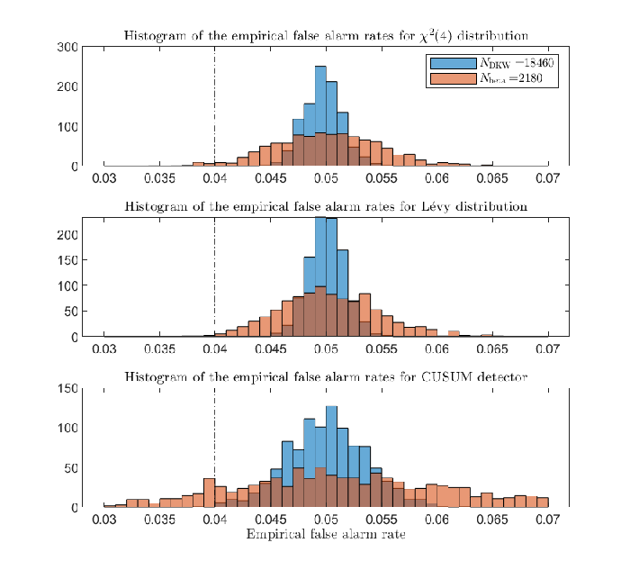
Fig. 3 shows the histogram of the empirical false alarm rate for the $\chi^{2}(4)$ distribution (upper plot), the Lévy distribution (center plot), and samples obtain from the CUSUM detector (lower plot) for each of the two sample sizes investigated. The two upper plots confirm our theoretical results, where the empirical false alarm rate lies inside the desired interval with a probability larger than $95\,\%$. More specifically, when $N=N_{\mathrm{beta}}$ and $y_{D}$ has a $\chi^{2}$ distribution only $4.2\,\%$, that is, $42$ out of $1000$, of the empirical false alarm rates are outside of the desired interval. Similarly, when $N=N_{\mathrm{beta}}$ and $y_{D}$ has a Lévy distribution only $2.4\,\%$ of the empirical false alarm rates are outside of the desired interval. If $N=N_{\mathrm{DKW}}$ none of the empirical false alarm rates are outside of the desired interval. Therefore, we see that the sample size provided by Theorem 2 are very close to the desired guarantees of at most $5\,\%$ of false alarm rates being outside the desired interval, while the sample size provided by Proposition 1 has much better probabilistic guarantees but has also a conservative amount of samples. Furthermore, the two upper plots in Fig. 3 verify that the guarantees hold for both light-tailed and heavy-tailed distributions.

However, in the lower plot, where the samples are not i.i.d., we observe that $34.1\,\%$ of the empirical false alarm rates lie outside of the desired interval when $N=N_{\mathrm{beta}}$ is used. For $N=N_{\mathrm{DKW}}$ only $0.3\,\%$ of the empirical false alarm rates lie outside the desired interval. Hence, we see that the probabilistic guarantees are not fulfilled, when $N=N_{\mathrm{beta}}$. Although in this case the choice of $N=N_{\mathrm{DKW}}$ provides enough conservatism to outweigh the effect of the non-i.i.d. sampling, in principle there is no guarantee in either case. Therefore, the sample size obtained in Theorem 2 is the smallest sample size that fulfills the probabilistic guarantees given $N_{\mathrm{beta}}$ i.i.d. samples, but it is sensitive to violations of the i.i.d. assumption.

One reasonable approach to deal with correlated data is to collect more data than the minimum amount for i.i.d. data and randomly sample an approximately i.i.d. subset of the correlated data. Proposition 1, Theorem 1, and Theorem 2 can help with determining the size of the approximately i.i.d. subset of correlated data, but not the minimum size of the correlated data needed. Determining the minimum size of the correlated data set for threshold estimation needs further investigation and is an avenue for future work. This approach of dealing with correlated data is used in the next section, when we obtain samples from our experimental setup.

In this last section, we evaluate the sample guarantees provided by Theorem 2 with data obtained from an experimental setup, where a real process is controlled. The process used is the Temperature Control Lab (TCLab), which consists of two heaters and one temperature sensor for each heater (for more details see [22]). In the experimental setup we control both heaters to have a temperature of $40\,{}^{\circ}\mathrm{C}$. We implement an LQG controller, which is based on a linearized and discretized model around the steady-state temperature $40\,{}^{\circ}\mathrm{C}$ for both heaters. Here we use a sampling time of $1\,\mathrm{s}$ to obtain measurements. From the TCLab’s sensors we obtain two measurements, $y(k)\in\mathbb{R}^{2}$, and with the predicted sensor measurements $\hat{y}(k)$ from the steady-state Kalman filter inside the LQG controller the residual signal is $\bar{r}(k)=y(k)-\hat{y}(k)$. Here, $r(k)=\hat{\Sigma}^{-\frac{1}{2}}(\bar{r}(k)-\hat{\mu})$ serves as the input to (10), where $\hat{\mu}$ and $\hat{\Sigma}$ are approximations of the mean and the covariance matrix of the residual signal, respectively, used to normalize $\bar{r}(k)$, $\delta=3$ in (10), and the initial state of the CUSUM detector is again set to zero. Note that, to the best of our knowledge, there exists no closed-form solution for the threshold of a CUSUM detector that guarantees an acceptable false alarm rate $1-\gamma$. Therefore, we will use $N_{\mathrm{beta}}$ samples of the detector to approximate the threshold according to (2) with $\beta=0$ for an acceptable false alarm rate of $1-\gamma$.

We let the experiment run for $15379\,\mathrm{s}$ to gather data. Since the detector output is assumed to be a random variable with a fixed distribution (see Assumption 1), we only work with samples from the steady state of the system, which is approximately reached for $k\geq 780$. We obtain $\hat{\mu}$ and $\hat{\Sigma}$ from the first 1000 samples of the residual signal in steady state, i.e., the data set $\mathcal{D}_{\mu\Sigma}=\{r(k)\}_{k=780}^{1779}$. With $\hat{\mu}$ and $\hat{\Sigma}$ available we determine the detector output $y_{D}(k+1)$ such that we use the data set $\mathcal{D}=\{y_{D}(k)\}_{k=1779}^{15379}$ of detector outputs to estimate the threshold, where $y_{D}(1779)=0$, and validate the empirical false alarm rate of the threshold estimate.

In the following, we apply the approach outlined at the end of the previous section. This means that, for a given $\gamma$, we randomly choose $N_{\mathrm{beta}}$ samples from $\mathcal{D}$ without replacement to obtain an approximately i.i.d. data set for determining $\tilde{J}_{D}$. Since we only have a finite amount of samples in $\mathcal{D}$, the remaining samples of $\mathcal{D}$ are compared to the threshold to produce the empirical false alarm rate induced by $\tilde{J}_{D}$. Repeatedly applying this approach is known as Repeated Training/Test Splits [23], which lets us simultaneously estimate and evaluate $\tilde{J}_{D}$ with a finite data set $\mathcal{D}$. This is done repeatedly to obtain $N_{T}=10000$ empirical false alarm rates for a given $\gamma$. For tuning the detector, we choose $\epsilon=0.01$ and $\rho=0.05$ and investigate nine different values for $\gamma$, that is, $\{\gamma_{i}\}_{i=1}^{9}$, where $\gamma_{i}=0.95+(i-1)\cdot 0.005$. For these values of $\epsilon$ and $\rho$, the amount of samples for testing is at least $11421$ for each of the investigated values of $\gamma$.

Fig. 4 shows a box plot of the empirical false alarm rates over the investigated acceptable false alarm rates $1-\gamma$. We observe that the median value of the empirical false alarm rate is almost exactly located at the acceptable false alarm rate for all investigated values of $\gamma$. Furthermore, the box plots are concentrated around the acceptable false alarm rate. Only $5\,\%$ of the empirical false alarm rates should lie outside of the $\pm\epsilon$-band (shaded area in Fig. 4) around the acceptable false alarm rate, since $\rho=0.05$. Here, the largest percentage of empirical false alarm rates outside the $\pm\epsilon$-band is $4.77\,\%$ for an acceptable false alarm rate of $0.045$, i.e., $\gamma=0.955$. Hence, although the data in $\mathcal{D}$ is strongly correlated due the CUSUM detector dynamics (10), the theoretical guarantees from Theorem 2 hold. The reason for that is that due to the random selection of $N_{\mathrm{beta}}$ samples from $\mathcal{D}$ to determine $\tilde{J}_{D}$, it is unlikely that several adjacent samples, e.g., $y_{D}(2000)$, $y_{D}(2001)$, and $y_{D}(2002)$, are chosen such that the samples in the training set are not highly correlated anymore.

Note that the samples in the test set are still strongly correlated. This shows that the guarantees for the threshold determined from the uncorrelated samples holds for the correlated samples in the test set as well.

Finally, we look at the histogram of the empirical false alarm rates for $\gamma=0.95$ (see Fig. 5). We observe that in contrast to the lower plot in Fig. 3 the histogram for $N=N_{\mathrm{beta}}$ is now concentrated around $1-\gamma=0.05$ and only $4.64\,\%$ of the empirical false alarm rates are located outside of the desired interval marked by the vertical dash-dotted lines. This demonstrates that by selecting training data using random sampling (as opposed to sequential sampling) we are able to employ the sample guarantees in Theorem 2 to find a threshold for the highly correlated output of the CUSUM detector.

References

- [1] J. Minkel. (2008, August) The 2003 Northeast Blackout–Five Years Later. (accessed: 12th of August 2020). [Online]. Available: https://www.scientificamerican.com/article/2003-blackout-five-years-later/
- [2] R. M. Lee, M. J. Assante, and T. Conway, “Analysis of the cyber attack on the Ukrainian power grid. defense use case,” E-ISAC, 2016.
- [3] J. W. R. McIntyre, “Ergonomics: Anaesthetists’ use of auditory alarms in the operating room,” International journal of clinical monitoring and computing, vol. 2, no. 1, pp. 47 – 55, 1985.
- [4] C. D. Brown and H. T. Davis, “Receiver operating characteristics curves and related decision measures: A tutorial,” Chemometrics and Intelligent Laboratory Systems, vol. 80, no. 1, pp. 24 – 38, 2006.
- [5] D. I. Urbina, J. A. Giraldo, A. A. Cárdenas, N. O. Tippenhauer, J. Valente, M. Faisal, J. Ruths, R. Candell, and H. Sandberg, “Limiting the impact of stealthy attacks on industrial control systems,” in Proceedings of the 2016 ACM SIGSAC Conference on Computer and Communications Security, ser. CCS ’16. New York, NY, USA: ACM, 2016, pp. 1092–1105.
- [6] V. Chandola, A. Banerjee, and V. Kumar, “Anomaly detection: A survey,” vol. 41, no. 3, July 2009.
- [7] N. Goix, “How to evaluate the quality of unsupervised anomaly detection algorithms?” ArXiv, vol. abs/1607.01152, 2016.
- [8] R. J. Hyndman and Y. Fan, “Sample quantiles in statistical packages,” The American Statistician, vol. 50, no. 4, pp. 361–365, 1996.
- [9] D. Umsonst, J. Ruths, and H. Sandberg, “Sample-based anomaly detector tuning with finite sample guarantees,” in 2021 American Control Conference (ACC), May 2021.
- [10] P. Massart, “The tight constant in the Dvoretzky-Kiefer-Wolfowitz inequality,” Ann. Probab., vol. 18, no. 3, pp. 1269–1283, 07 1990.
- [11] F. Pukelsheim, “The three sigma rule,” The American Statistician, vol. 48, no. 2, pp. 88–91, 1994.
- [12] M. Thulin, “The cost of using exact confidence intervals for a binomial proportion,” Electron. J. Statist., vol. 8, no. 1, pp. 817–840, 2014.
- [13] C. Murguia and J. Ruths, “CUSUM and chi-squared attack detection of compromised sensors,” in 2016 IEEE Conference on Control Applications (CCA), Sept 2016, pp. 474–480.
- [14] V. Renganathan, N. Hashemi, J. Ruths, and T. H. Summers, “Higher-order moment-based anomaly detection,” IEEE Control Systems Letters, pp. 1–1, 2021.
- [15] D. Li and S. Martínez, “High-confidence attack detection via Wasserstein-metric computations,” IEEE Control Systems Letters, vol. 5, no. 2, pp. 379–384, 2021.
- [16] S. Clémençon and J. Jakubowicz, “Scoring anomalies: a M-estimation formulation,” ser. Proceedings of Machine Learning Research, C. M. Carvalho and P. Ravikumar, Eds., vol. 31. Scottsdale, Arizona, USA: PMLR, 29 Apr–01 May 2013, pp. 659–667.
- [17] R. Rockafellar and S. Uryasev, “Conditional value-at-risk for general loss distributions,” Journal of Banking & Finance, vol. 26, no. 7, pp. 1443 – 1471, 2002.
- [18] A. Okolewski and T. Rychlik, “Sharp distribution-free bounds on the bias in estimating quantiles via order statistics,” Statistics & Probability Letters, vol. 52, no. 2, pp. 207–213, 2001.
- [19] H. A. David and H. N. Nagaraja, Order Statistics, 3rd ed. Wiley, 2003.
- [20] Handbook of beta distribution and its applications, ser. Statistics: textbooks and monographs ; 174. New York: Marcel Dekker, 2004.
- [21] A. Papoulis, Probability, random variables, and stochastic processes, 3rd ed., ser. McGraw-Hill series in electrical engineering Communications and signal processing. New York: McGraw-Hill, 1991.
- [22] J. Park, R. A. Martin, J. D. Kelly, and J. D. Hedengren, “Benchmark temperature microcontroller for process dynamics and control,” Computers & Chemical Engineering, vol. 135, p. 106736, 2020.
- [23] M. Kuhn and K. Johnson, Over-Fitting and Model Tuning. New York, NY: Springer New York, 2013, pp. 61–92.