Generalized Hessian-Schatten Norm Regularization for Image Reconstruction
Abstract
Regularization plays a crucial role in reliably utilizing imaging systems for scientific and medical investigations. It helps to stabilize the process of computationally undoing any degradation caused by physical limitations of the imaging process. In the past decades, total variation regularization, especially second-order total variation (TV-2) regularization played a dominant role in the literature. Two forms of generalizations, namely Hessian-Schatten norm (HSN) regularization, and total generalized variation (TGV) regularization, have been recently proposed and have become significant developments in the area of regularization for imaging inverse problems owing to their performance. Here, we develop a novel regularization for image recovery that combines the strengths of these well-known forms. We achieve this by restricting the maximization space in the dual form of HSN in the same way that TGV is obtained from TV-2. We name the new regularization as the generalized Hessian-Schatten norm regularization (GHSN), and we develop a novel optimization method for image reconstruction using the new form of regularization based on the well-known framework called alternating direction method of multipliers (ADMM). We demonstrate the strength of the GHSN using some reconstruction examples.
Regularization, Total Variation, Total Generalized Variation, Hessian-Schatten Norm, Inverse Problems, MRI Reconstruction.
1 Introduction
Images acquired using different imaging devices are inevitably corrupted due to the physical limitations of the image formation model. An estimation scheme [1] that employs knowledge of the image formation forward model to generate a better quality estimate is known as image restoration/reconstruction [2]. The relative improvement in the image quality obtained by image restoration/reconstruction is typically significant in most modalities in general, and in particular, in modalities such as MRI imaging [3, 4], computed tomography [5, 6], confocal microscopy [7] and widefield microscopy [8]. One of the classical approaches to image restoration is the regularized approach [9]. It formulates the required reconstruction by means of the solution to the optimization problem as given below:
| (1) |
where is the data fitting functional that measures the goodness of fit of the candidate image , to the measured image , and is the regularization functional that measures some kind of roughness of the image. The structure of data fitting term is dependent on the forward model of the imaging device and the assumed statistical model of the noise. The regularization functional [10] represents the prior information we have about the class of images we are trying to restore. The constant term is a user parameter that allows a trade off between the regularization term and the data fitting term.
Design of regularization functional is a long-studied problem in signal and image processing [2]. One of the classic regularization techniques is Tikhonov regularization [11]. Tikhonov regularization was originally employed for solving integral equations, but it proved to be successful in imaging inverse problems [12] as well. The earliest form of Tikhonov regularization was constructed using sum-of-squares of the candidate image/signal [11], and then the later forms were constructed using sum-of-squares of image/signal derivatives. Derivative based Tikhonov regularized reconstruction can be expressed as
| (2) |
where and are filters implementing first order derivatives, , and respectively. The main advantage of using Tikhonov regularization is that the required reconstruction can be expressed in terms of linear system of equations when the data fitting term is also quadratic. However, Tikhonov regularization leads to over-smooth solutions. Nevertheless, Tikhonov regularization is still widely used epspecially in large scale problems such 3D deconvolution [13]. It was generally believed that non-linear methods gave better quality reconstructions, and the earliest forms of regularizations that led to non-linear methods were based on norm of the wavelet transform of the candidate image. Representative methods in this category include ISTA [14, 15, 16], FISTA [17] and TwIST [18]. These methods are primarily based on the fact that wavelet transform of typical images have low norm. The basis used in the wavelet transform can be adapted to data to give better performance in image restoration problems [19]. It should be emphasized that the factor that makes wavelet regularization better than the Tikhonov is that the wavelet transform has inbuilt derivatives and hence wavelet regularization in some sense becomes equivalent to minimization image derivatives. This leads to better preservation of structures than Tikhonov regularization which smooths out edges due to minimization of derivatives.
The seminal work by Rudin, Osher and Fatemi demonstrated that minimization of norm of image derivatives, in particular gradients, leads to better preservation of image structures [20]. This regularization is called total variation (TV) regularization and its practical and theoretical advantages have been well demonstrated [21, 22, 23]. This makes total variation an active area of research even after decades of discovery. TV regularized image reconstruction can be expressed as
| (3) |
For a rigorous treatment of Total Variation (TV), the reader can refer to [24]. TV regularization has been widely used [25, 26, 27, 28, 29] because of its ability to recover sharp image features in the presence of noise and in the cases of under-sampling. While TV can retain edges [20] in the reconstruction as compared to Tikhonov regularization [24], and in particular, it can recover sharp jumps in the reconstruction even in the presence large amount of noise and/or undersampling. At the same time it has a disadvantage that, in the presence of large amount of noise and/or undersampling, it approximates smooth intensity variations in terms of piece-wise constant segments, which is known as staircase artifacts [30]. Higher order extensions of TV [30] have been proposed to avoid staircase effect and they deliver better restoration. Second order TV (TV-2) [31, 32, 33] restoration was proposed as
| (4) |
where , and are discrete filters implementing second order derivatives , and respectively. TV-2 recovers linear intensity variations in the presence large amount of noise and/or undersampling; it looses the ability to reproduce sharp intensity jumps that TV-1 can recover. Another second-order derivative based formulation is Hessian-Schatten (HS) norm regularization [34], which has been proposed as a generalization of the standard TV-2 regularization. It is constructed as an norm of eigenvalues of the Hessian matrix, which becomes the standard TV-2 for . HS norm with has been proven to yield best resolution in the reconstruction, since this better preserves eigenvalues of the Hessian [34]. Let and let be the operator that returns the vector containing the eigenvalues of its matrix argument. Then HS norm regularization of order is expressed as
| (5) |
Since the eigenvalues are actually directional second derivatives taken along principle directions, setting better preserves the local image structure.
Papafitsoros et al. proposed a regularization method that combines both first- and second-order derivatives [35]. The reconstruction problem is formulated as given below,
| (6) |
where and are user parameters that determine the relative weight. A generalization for total variation to higher order terms, named as total generalized variation (TGV) has also been proposed [36]. It is generalized in two ways: it is formulated for any general derivative order; for any given order, it is generalized in the way how the derivatives are penalized. The second form of generalization is obtained by expressing the standard total variation regularization in dual form as a maximization, and then by imposing spatial smoothing constraint in the maximization problem. The second aspect of generalization has more significant impact in practical point of view. In fact, the version of TGV regularization that has been applied for non-trivial inverse problems (problems other than denoising) obtained by restricting the maximum order to be two; compared to most widely used TV-2 regularization, it differs only by the second aspect of generalization. This form of regularization is called second order TGV (TGV-2) and takes the following form:
| (7) |
where is an auxiliary vector image. The TGV-2 functional is able to spatially adapt to the underlying image structure because of the minimization w.r.t. auxiliary variable . Near edges, approaches zero leading to TV-1-like behaviour which allows sharp jumps in the edges. On the other hand, in smooth regions, approaches leading to TV-2-like behaviour which will avoid staircase artifacts. This means that TGV-2 combines the best of TV-1 and TV-2 regularizations. However, the drawback with TGV functional is that the weights and have to be chosen by the user.
The recent leap in the computing power of desktop computers led the application deep neural networks (DNN) for image restoration [37]. These DNN based image restoration methods can be categorized into two types. In the first category, a map (composed of multi-layer neural networks) that can estimate underlying image from measured image is learned from the several training pairs, where each pair has a measured image and the underlying image that generated the measured image. Note that this map plays dual role: it accounts for stable inversion of imaging forward model, and encompasses prior knowledge of typical ground truth images. This type of DNN methods were applied for MRI image restoration [38, 39], CT image [40] reconstruction, image deconvolution [41] and other imaging inverse problems. In the second category, only the effect of noise is learned. Therefore, these maps are known as denoisers and plugged as a module in a variable splitting optimization scheme (e.g., Primal-Dual splitting). Some prominent works of this category are [42] and [43]. The main argument that supports the use of DNN is that, while regularization methods impose adhoc prior beliefs on the image to be restored, a trained DNN encompasses a more natural knowledge resulting from training data. However, a recent work by Hansen et al. [44] shows that such learned maps can be unstable. Further, need for large amount of training data limits the applicability of DNN based methods.
In this paper, we develop a novel type of regularization by generalizing the Hessian-Schatten norm regularization in the same way that TGV-2 regularization generalizes the TV-2 regularization. The resulting form of regularization includes TV-2, TGV-2, and Hessian-Schatten norm regularization as special cases. We call this regularization as the generalized Hessian-Schatten norm regularization (GHSN). Next, we develop a novel optimization method for image reconstruction using the GHSN and demonstrate the effectiveness of GHSN regularization using numerical experiments involving reconstructions from sparse Fourier samples.
Notations and mathematical preliminaries
- 1.
Vectors are represented by lower-case bold faced letters with the elements represented by the same letter with a subscripted index. For example, denotes a vector and its th element is denoted by . For a vector , denotes the norm given by . It can be shown that with converges to the component of that has the largest magnitude, and hence we write .
- 2.
We will deal with vector images; vector images are discrete 2D arrays where each pixel location has a vector quantity. It is denoted by lower-case bold-faced letter with a bold-faced lower-case letter as an argument. For example, is a vector image with representing a 2D pixel location. Depending on the context, the symbol denoting the pixel location may be omitted.
- 3.
For a vector image, , denotes . It is the sum of pixel-wise norms, where denotes the sum across pixel indices. Throughout the paper, we do not specify the bounds of summation as it is always the same and ranges from the first to last pixels. The norm is a composition of two norm, and is called the mixed-norm.
- 4.
Matrices are represented by upper case bold faced letters. For a matrix , denotes the Frobenius norm, which equal to the square root of sum of squares of its elements; it can be written as , where denotes the summing of diagonal elements. Next denotes the Schatten p-norm of the matrix, which is the norm of the vector of singular values of the matrix . For a symmetric matrix, it is also the same as the norm of the Eigen values. In other words, if denotes the operator that returns the vector of eigenvalues of a matrix, then .
- 5.
We will also deal with matrix images; matrix images are discrete 2D arrays where each pixel location has a matrix quantity. It is denoted by upper-case bold-faced letter with a bold-faced lower-case letter as an argument. For example, is a matrix image with representing a 2D pixel location. Depending on the context, the symbol denoting the pixel location may be omitted. For a vector image, , its th scalar image is given by . For a matrix image, , its th scalar image is given by .
- 6.
For an matrix image, , let denote the norm of the pixel-wise Schatten p-norms. In other words, we have . Further, let denote the norm of the pixel-wise Schatten p-norms. In other words, we have . Note that the norms and are mixed-norm.
- 7.
For square matrices of same dimension, , , let . For a square matrix let . Then the following holds for any pair of square matrices: .
- 8.
If , and denote matrix images such that for each pixel index , , and denotes square matrices of the same dimensions, then, denotes . On the other hand, denotes .
- 9.
For a matrix image , the norm can be expressed as a maximization of inner product of the form [34]. Specifically we can write
(8) where is the real positive number satisfying . The notation denote maximization within the set of matrix images with the value of mixed norm upper-bounded by .
- 10.
In this paper, * denotes the 2-D convolution operation, i.e We extend notion of convolution to matrix images by using the rules of matrix multiplication. To be more specific, let be an image of matrices and let be image of matrices. Then, for . As an example, let both and be matrix images. Then the elements of , can be written as
- 11.
For a scalar image and an image of matrices, , is defined as for , and any location .
- 12.
For an image of matrices, , we can define a new matrix image by extending the idea of transpose of a matrix to the case of matrix images. The entry of can be defined as for , and any location .
- 13.
For scalar images and , and a scalar filter , the convolved inner product satisfies the relation , where denotes the flipped filter, i.e., satisfies . This relation can be easily verified by writing the inner product in Fourier domain.
- 14.
We will extend the notion of flipping for vector filter in a straight forward way. In other words, for a vector filter , denotes the vector filter obtaining by flipping each of its constituent scalar filters. For a vector image and a vector filter , and a scalar image of appropriate size, , we have . The operation is the adjoint of the operation .
- 15.
Let be an matrix image, and let and be vector filters. Then using the ideas of the previous point, we can show that . By a trivial extension of this relation, we can also show that for any scalar image .
- 16.
Let where and denote discrete filters implementing the derivative operators and . Then for a scalar image, , is the discrete gradient of . Its adjoint, , which is defined for image of vectors, is called the discrete divergence. For a vector image , we write .
- 17.
The extension of the notion of gradient for vector images is called the Jacobian. For a vector image, , the Jacobian is given by . For a vector image, , and matrix image, , the inner product satisfies where is the row vector image obtained by applying the adjoint of the operation on . is given by .
2 Generalized Hessian-Schatten norm regularization
Let be the discrete candidate image, where is the discrete pixel index. Recall that, denotes the discrete Hessian operator. Convolution of this operator with (denoted by ) is the discretized Hessian of the candidate image. We regard as an image of matrices; in other words, for each pixel index, , is a matrix. Using this formulation, the well-known second-order total variation regularization can be expressed as . Similarily, Hessian-Schatten norm regularization [45] of order applied on the candidate image can be expressed as
| (9) |
To develop the novel regularization by extending Hessian-Schatten norm, we use the dual form of the Schatten norm. Specifically, we write Hessian-Schatten norm on as
| (10) |
Note that the above maximization is within the space of matrix images. The maximizer will be a symmetric matrix image, because the Hessian, , is symmetric. Hence, will also be equal to the result of maximization within the space of symmetric matrix images. This is again equivalent to writing
| (11) |
To formulate the generalization, we write the above expression in expanded form given below:
| (12) |
From the above form, it is clear that the maximization is carried out for each independently. Suppose denotes the set of symmetric matrices such that, for each we have . Then the above minimization is carried out within a set that has a size that is times the size of , where is the size of . We propose to generalize by restricting the maximization space in the same way the second order TGV generalizes the second order total variation regularization (TV-2) [36]. To this end, let be of the form , and let for a matrix image be as defined in Notations and mathematical preliminaries. Note that is vector image. With this, we express the generalization as given below:
| (13) |
By using the fact that and transposition does not affect norm, we can write as given below:
| (14) |
Note that is a generalization in the sense that is special case of , i.e., . The above form is not usable as a regularization for image recovery as it involves symmetrization operation. Further, directly using the above form will lead to min-max problem, which will not be very convenient for developing numerical minimization. Interestingly, the above form can be translated into a form that appears very close the form TGV-2 given in the equation (7) with the matrix Frobenius norm replaced by the Schatten norm. The following proposition gives this expression.
Proposition 1
The generalized Hessian-Schatten norm can be expressed by
| (15) |
Note that, in terms of pixel-wise summations, the above form of regularization can written as
| (16) |
Note that this form resembles with TGV-2 given in the equation (7), except the fact that is replaced by . By noting the fact that with becomes the same as , we conclude that the proposed regularization includes TGV-2 as a special case. Further note that becomes the Hessian-Schatten norm regularization as . Moreover, it becomes the TV-2 regularization with as . It can be observed that the new regularization combines the best of Hessian-Schatten norm regularization and TV-1 regularization, in the same way as TGV-2 combines the best of TV-1 and TV-2 regularization. Near edges, approaches zero leading to TV-1-like behaviour which allows sharp jumps in the edges. On the other hand, in smoother regions, approaches leading to the structure preserving ability of Hessian-Schatten norm.
3 Image reconstruction algorithm using GHSN regularization
3.1 The cost function
In our development, we will restrict the image measurement model to be in convolutional form. We do this to gain the convenience in implementing the forward model, as our main focus is on the regularization. Let denote the impulse response of the imaging system and suppose that the noise is Gaussian. We allow the possibility that can be complex, and hence the measurement can have complex values. With this, the data fitting term is given by , and the GHS regularized image reconstruction can be expressed as
| (17) |
By accounting for the fact that itself is expressed via a minimization, we can also write the above problem as,
| (18) |
where
| (19) |
For notational convenience in developing the minimization algorithm, we re-express the cost in terms of the combined variable . To this end, we define the following:
| (20) | ||||
We will overload the notation , such that when used with a vector as the argument, it represent the following:
Let be the matrix such that . With these, the overall cost to be minimized can be expressed as
| (31) |
Note that definition of creates an additional scale factor of in the middle term in eq. 31. But, this does not create any difference in the formulation as is an independent parameter, which is tuned for optimum reconstruction quality. Hence we absorb the scaling into the parameter . Henceforth, the weight parameter in the middle term will be instead of .
Note that with is the well-known TGV-2 regularization. Guo et al. [46] developed an algorithm for image reconstruction using TGV-2 and shearlet regularization. With the shearlet part removed, their algorithm corresponds to the following constrained formulation of the reconstruction problem:
| (32) | ||||
The main advantage of this form is that the ADMM algorithm can be constructed using well known proximal operators. However, the algorithm can be badly conditioned in some cases as we will demonstrate in the experiment section.
3.2 Proposed ADMM algorithm
Before specifying the variable splitting scheme for the proposed ADMM algorithm, we first rewrite the cost of the equation (31) as
| (33) |
where is the bound constraint function, which takes infinity when any of the pixel of is outside the user-defined bound and zero otherwise, and with denoting Kronecker delta, and hence . We propose to build ADMM algorithm by means of the following constrained formulation:
| (34) | ||||
The main difference from the previous formulation [46] is that the matrices and are not a part of the constraints, but, are left as a part of the cost to be minimized. This leads to some numerical advantages, which we will clarify after completing the development of the algorithm. On the other hand, this splitting scheme requires constructing new proximal operators for implementing the ADMM algorithm. We do this in the next section which is one of the important contributions of the paper. In the remainder of this section, we complete specifying the ADMM iteration for splitting scheme specified above. In order to facilitate developing algorithm in terms of compact expressions, we need to further simplify the notations. To this end, let
| (35) | ||||
With this, the above problem can be expressed as
| (39) | ||||
| (40) |
where
| (41) |
The next step towards developing the ADMM algorithm is to write the augmented Lagrangian of the above constrained optimization problem. The augmented Lagrangian is given by
| (42) |
where is vector image of Lagrange’s multiplier with its dimension equal to that of . Also, is a fixed positive real number. The ADMM becomes series of minimizations with respect to and and updates on . Given the current set of iterates, the ADMM methods proceeds as follows:
| (43) | ||||
| (44) | ||||
| (45) |
4 Solving the sub-problems of ADMM
4.1 The -problem
4.1.1 Expressing the pixel-wise sub-problems
Note that the solution to the minimization problem of equation (43), , is also the minimum of the following cost:
| (46) |
where,
| (47) |
For notational convenience, let and let . Note that the cost is separable across the subvectors of the variable, ; in other words, it is separable across the subvectors , , and , and we introduced the collective variable, only for notational convenience in expressing the ADMM loop of equations (43), (44), (45). As we are focused on this specific sub-problem, we will now separate the constituent problems. To this end, let , , and denote the sub-vectors of conferring to the partitioning given in the equation (35). Similarly, let , , and be the subvectors of . With this the solution to the -problem can be expressed as
| -problem: | (48) | |||
| -problem: | (49) | |||
| -problem: | (50) |
Note that the functions , , and are separable across pixel indices since they are constructed as mixed norms composed elementary pixel-wise norms. Hence, they can be expressed as a sum of pixel-wise elementary functions. The form of these elementary functions can be clearly deduced from the form of the functions , , and . We can express these functions as
| (51) | ||||
| (52) | ||||
| (53) |
From the above form, it is clear that the minimization problems are separable across pixel indices. Hence the solution to the minimization problems of equations (48), (49), and (50), can be expressed as the following:
| (54) | ||||
| (55) | ||||
| (56) |
4.1.2 Solution to the pixel-wise sub-problems
The solution to the -problem is very simple, and it is the clipping of the pixels by bound that defines [47]. We express the solution as given below:
| (57) |
where denotes the operation of clipping the pixel values within the specified bounds. Next, we consider expressing the solution for -problem. Note that, in the absence of the matrix , the solution will be the well-known shrinkage operation on the norm of [47]. Because of the presence of the matrix, , the shrinkage operation is not directly applicable. The following proposition gives the solution to the problem.
Proposition 2
The minimum of with respect to is given by , where .
Now, considering the problem, i.e., considering the minimization of , the presence of makes the problem more complex. Otherwise, the solution to the problem in the absence of is well-known [48]. The following proposition gives expression for solution to this problem.
Proposition 3
The minimum of with respect to is given by where represents the minimum of the with respect to , and and is the matrix such that its operations on is defined as .
Note that is the well-known proximal operator of Schatten norm (for details see [48]), and the above proposition expresses the required proximal operator—proximal operator for the modified Schatten norm, —as a simple modification of . Note that we just need set for applying the above proposition for the problem of equation (55). Although is well known, in Algorithm 3, we provide detailed description of to the level required for implementation along with a self-contained description of the overall algorithm. Note that, we have non-iterative exact formula for only for . Hence, in the experimental demonstration, we only consider these two values for .
4.2 The -problem
Now we consider the minimization problem of equation (44). By taking the dependencies of the minimization variable , it can be deduced that, the solution to this problem is also the minimum of the following cost function:
| (58) |
where
| (59) |
As done before for notational convenience, we let , and . Let , . From the definition of given in the equation (3.2), and from the definition of , it is clear that the cost is separable across the components of , which are , , and . They are given below:
| (60) | ||||
| (61) | ||||
| (62) |
Here, . These are quadratic functions involving simple discrete filtering operation. Hence, their minima can be expressed in terms of simple Fourier inversion. To this end, we write the expression for the gradients below:
| (63) | ||||
| (64) | ||||
| (65) |
In the above equation, represents pointwise complex conjugate operation. Now, the minima , , and can be obtained by solving , , and in Fourier domain. This is the main advantage of the proposed variable splitting: we are able to solve for , , and independently by simple Fourier division. On the other hand, the -problem encountered in the splitting proposed in [46], the components , , and are coupled, and hence, it requires solving system of equations each of frequencies values where is the size of the image to be reconstructed. The linear system to be solved in the sub-problem do not have a block diagonal structure as obtained in our version of ADMM algorithm. Instead we need to solve a non-diagonal block circulant system. Although the required inverses can be precomputed outside the ADMM loop, it turns out that overall numerical conditioning is worse than the splitting that we propose here, which we demonstrate experimentally in Section 5. In Algorithm 1, we provide detailed expression of the solutions of , , and to the level required for implementation. Algorithm 1 also serves as the self-contained specification of the overall proposed reconstruction method.
: measured image
: Impulse response of imaging system
: regularization weight for first order term
: regularization weight for second order term
: termination tolerance
Symbol definitions: and are first derivative filters
and are flipped versions
is flipped version of
, ,
while do
(Clipping of elements)
end while
: vector image corresponding to first order derivative
: vector image corresponding to second order derivative
: regularization weight for second order term
: regularization weight for second order term
for do
end for
end if
5 Experiments
Recall that we have two main contributions in this paper: (i) a generalization of Hessian-Schatten -norm [34] with the resulting form that also generalizes second order total generalization variation regularization (TGV-2) [36]; (ii) a novel ADMM based reconstruction algorithm with improved numerical behaviour owing to the novel variable splitting scheme. Implementing the algorithm with novel variable splitting is enabled by novel proximal operators derived in this paper. The goal of this section is to demonstrate the role of both of these contributions in improving the quality of reconstruction. To this end, we consider the problem of reconstructing images from quasi-random Fourier samples. We use the images given in fig. 1 as the models. To obtain quasi-random Fourier samples, we use the trajectories generated by solving travelling salesman problem as proposed by Chauffert et al [49]. Sampling trajectories corresponding to two sampling densities were used, which are given in fig. 2. The first one covers of the samples in the Fourier plane whereas the second trajectory covers . We restrict to be in .
As done by Chauffert et al [49], we quantize the sample locations generated from such trajectories by the grid corresponding to the DFT of the image. This helps with the fast implementation of the algorithms. Suppose denotes the operation of obtaining the vector of Fourier samples from the quantized Fourier locations, and let be the vector of complex Fourier samples. Since the noise is Gaussian, the negative log likelihood of the measurement model is given by . It can be shown that we have the following relation: , where represents inverse DFT of zero-embedded Fourier measurements, , and represents inverse DFT of the image that has ones corresponding to Fourier sampling locations, and zeros everywhere else. Note that and will typically be complex. In summary, the algebraic form of algorithm developed in Section 3.1 matches with the measurement model considered in our experiments.


5.1 Experiment 1
In this experiment, the goal is to show the advantage of both the contributions described above. To this end, we consider three forms of reconstruction methods that differs from each other in terms of regularization and/or the minimization methods:
- •
GHS-1: Reconstruction using the Generalized Hessian Schatten norm with and with proposed ADMM method for minimization
- •
GHS-2: Reconstruction using the Generalized Hessian Schatten norm with and with proposed ADMM method for minimization
- •
GHS-2(G): Reconstruction using the Generalized Hessian Schatten norm with with optimization method proposed by Guo et al. [46]
Note that, in GHS-2, the regularization is the same as the TGV-2 [36]. This means, GHS-2 has novelty only in terms of optimization used, whereas GHS-1 has novelty both in terms of the regularization and the optimization method. GHS-2(G) entirely corresponding the method of Guo et al [46] with the part corresponding to the additional wavelet regularization removed. To evaluate these methods, we generated test dataset from all given images by using the transfer function TF1. The Fourier samples were corruption by additive white Gaussian noise with variance 4. Table 1 compares PSNR score of reconstruction obtained from all three methods with 500, 1500, and 10000 iterations. It is clear from the table that GHS-1 gives the best score with all three cases of number of iterations for most cases of measured images, and GHS-2 comes next in PSNR. The PSNR score of GHS-2(G) is always the lowest. By considering the fact that GHS-2(G) differs from GHS-2 only by optimization, we conclude that the proposed ADMM method is more efficient than the optimization method proposed by Guo et al [46]. We further note that, beyond 1500 iterations, there is no further improvement in the reconstructed image, and there is always a difference between the reconstruction obtained by GHS-2 and GHS-2(G). This confirms that the proposed ADMM method is better conditioned numerically. Considering the average time required for a single iteration, all methods take comparable amount of time.
| Image | Algorithm | 500 Iter. | 1500 Iter. | 10000 Iter. |
| Image 1 | GHS-2(G) | 32.52 | 32.53 | 32.53 |
| GHS-2 | 32.64 | 32.66 | 32.66 | |
| GHS-1 | 33.36 | 33.37 | 33.37 | |
| Image 2 | GHS-2(G) | 36.79 | 36.79 | 36.79 |
| GHS-2 | 36.90 | 36.92 | 36.92 | |
| GHS-1 | 37.24 | 37.25 | 37.25 | |
| Image 3 | GHS-2(G) | 35.92 | 35.92 | 35.92 |
| GHS-2 | 35.98 | 35.98 | 35.98 | |
| GHS-1 | 36.27 | 36.27 | 36.27 | |
| Image 4 | GHS-2(G) | 32.88 | 32.88 | 32.88 |
| GHS-2 | 32.89 | 32.92 | 32.92 | |
| GHS-1 | 33.19 | 33.21 | 33.21 | |
| Image 5 | GHS-2(G) | 30.11 | 30.22 | 30.22 |
| GHS-2 | 30.14 | 30.24 | 30.24 | |
| GHS-1 | 30.00 | 30.27 | 30.27 | |
| Image 6 | GHS-2(G) | 41.77 | 42.12 | 42.12 |
| GHS-2 | 41.87 | 42.15 | 42.15 | |
| GHS-1 | 41.61 | 42.13 | 42.13 |
5.2 Experiment 2
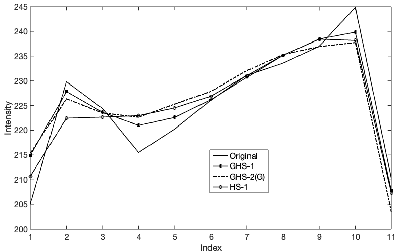
In the second set of experiments, we demonstrate the importance of novel regularization and the novel optimization under varied input settings. To this end, we simulate measurement data sets using both transfer function and add complex Gaussian noise on the Fourier samples with standard deviation values 5 and 7, which will be referred to as noise levels 1 and 2. This makes a total of 24 measurement sets. We evaluate all three methods listed in the previous experiment. We also evaluate with two additional methods: (i) HS-1: reconstruction using Hessian-Schatten 1-norm regularization with ADMM based minimization; (ii) HS-2: reconstruction using Hessian-Schatten 2-norm regularization with ADMM based minimization. Note that Hessian-Schatten 2-norm regularization is also the same as TV-2 regularization. The results are displayed in Table 2. From the table, it is clear that GHS-1 is the best performing method. We also note that, among the three methods, GHS-1, GHS-2, GHS-2(G), we see the same pattern of relative performance as in the first experiment. Further, GHS-1 and GHS-2 are better than HS-1 and HS-2 most cases. Moreover, while GHS-2 is consistently better than HS-2, GHS-2(G) is not always better than HS-2, although its regularization is the same as that of GHS-2. As GHS-2 differs from GHS-2(G) only by the optimization technique, this again confirm the importance our novel optimization method. The images restored from the measurement simulated from image 1 using the transfer function TF1 with noise level 1 are displayed in fig. 3. We also display a zoomed-in region in each of the restored images. It is clear from the zoomed in images that GHS-1 and GHS-2 schemes better recovers the edges without any staircase effect. In fig. 4, we present scan-lines from this image. As it is difficult to have clarity in the plot if several scan-lines are shown, we chose to show scan-lines of reconstructions from three methods only along with the scan-line from the original image; we chose the best performing variant from the proposed method, GHS-1, and the closest competitors from the literature, GHS-2(G) and HS-1. The scan-lines confirms that GHS-1 follows the ground truth better than other methods.

| Name | TF | Noise Level | TV2 | HS | GHS-2 | GHS-1 | GHS-2(G) |
| Im 1 | TF1 | 1 | 31.41 | 31.80 | 31.37 | 31.88 | 31.27 |
| 2 | 30.78 | 31.10 | 30.76 | 31.17 | 30.66 | ||
| TF2 | 1 | 26.22 | 26.66 | 26.22 | 26.68 | 26.10 | |
| 2 | 26.00 | 26.36 | 26.00 | 26.44 | 25.88 | ||
| Im 2 | TF1 | 1 | 33.55 | 33.69 | 33.53 | 33.70 | 33.43 |
| 2 | 32.44 | 32.57 | 32.41 | 32.58 | 32.31 | ||
| TF2 | 1 | 29.20 | 29.37 | 29.15 | 29.30 | 29.08 | |
| 2 | 28.72 | 28.83 | 28.68 | 28.83 | 28.60 | ||
| Im 3 | TF1 | 1 | 34.27 | 34.38 | 34.23 | 34.38 | 34.15 |
| 2 | 33.63 | 33.72 | 33.59 | 33.72 | 33.52 | ||
| TF2 | 1 | 28.19 | 28.30 | 28.15 | 28.34 | 28.11 | |
| 2 | 28.04 | 28.12 | 27.96 | 28.10 | 27.92 | ||
| Im 4 | TF1 | 1 | 31.44 | 31.65 | 31.48 | 31.74 | 31.40 |
| 2 | 30.82 | 30.97 | 30.87 | 31.09 | 30.79 | ||
| TF2 | 1 | 26.01 | 26.24 | 26.43 | 26.47 | 26.35 | |
| 2 | 25.91 | 26.07 | 26.21 | 26.22 | 26.13 | ||
| Im 5 | TF1 | 1 | 28.81 | 29.19 | 28.93 | 29.23 | 28.93 |
| 2 | 28.43 | 28.78 | 28.41 | 28.81 | 28.34 | ||
| TF2 | 1 | 22.96 | 23.23 | 23.10 | 23.25 | 23.08 | |
| 2 | 22.85 | 23.12 | 22.96 | 23.16 | 22.92 | ||
| Im 6 | TF1 | 1 | 33.74 | 33.93 | 34.22 | 34.21 | 34.22 |
| 2 | 32.50 | 32.68 | 32.77 | 32.76 | 32.77 | ||
| TF2 | 1 | 28.82 | 28.97 | 29.31 | 29.30 | 29.29 | |
| 2 | 28.47 | 28.60 | 28.63 | 28.63 | 28.62 |
6 Conclusion
We proposed a new form of regularization named Generalized Hessian Schatten Norm (GHSN) regularization. GHSN generalizes all existing forms of second-order derivative based regularization. We also developed a novel ADMM optimization method for image reconstruction using GHSN. We demonstrated the advantage of the generality in GHSN experimentally. We also demonstrated the effectiveness of the novel optimization method. In particular, even when parameters of GHSN is restricted to such that it becomes the well known form, called second order total generalized (TGV-2) variation, our optimization method outperforms the optimization proposed for TGV-2 in the literature.
Appendix A: Proof of propositions
Proof of proposition 1
First we reproduce Eq. (14):
| (66) |
Next, we denote the set as and, as . This gives
| (67) |
Next, we note that , , and . This means that we have . Substituting this gives
| (68) |
By the property inner products with convolution, we can replace the operation applied on the second argument of the inner product by the adjoint operation applied on the second argument. This gives
| (69) |
Now, we can replace the maximization by the minimization of the negated function and obtain
| (70) |
The above minimization problem can be posed as constrained optimization problem as given below:
| (71) | ||||
Since the above problem is a convex optimization problem, can be determined using duality theory. To this end, we construct the Lagrange dual cost function of the minimization problem as given below:
| (72) |
The above problem can be rearranged as given below by separating the terms for and :
| (73) |
Next, we note that . This gives
| (74) |
By duality theory, since strong duality holds ([50], Proposition 6.4.2), we have . Hence, the cost can be expressed as
| (75) |
Next, we rewrite the maximization with respect to as the minimization:
| (76) |
As the part of the cost function with respect to and are separable, we can rewrite the respective maximizations independently as given below:
| (77) |
Now we apply the definition of conjugate norm. By noting the fact that the conjugate (dual) norm for the norm is with [51], and for is . Substituting this gives
which completes the proof.
Proof of proposition 2
First we note that , and let be matrix such that the augmented matrix satisfies . Further, let , and , and let and , where and are sub-vectors of of size , and similarly and sub-vectors of of size . Then the form of cost function that is easy to minimize can be obtained by substituting , , and in . By doing this, we obtain the transformed function as given below:
| (78) |
Let denote the minimum of . Clearly, . Next, is the well-known proximal solution of norm [47], and it is given by , where . From these, the minimum of , denoted by can be expressed as . By replacing by , we get . Next, from the expression for , we can deduce the following on the difference :
By using the above relation and by using the fact that , we get
Substituting in the above expressing gives the final expression.
Proof of proposition 3
From the definitions of and , we first note that they can be expressed as
| (79) |
From the form given above, we observe that , , and . Hence, can be written as . As a result, the minimization problem becomes,
As an additional property, we also observe that . Hence, we have . This means that the minimum of , denoted by , can be written as , where
Next, because of the relation , we have . This means that the minimization subproblem can be separated as
| (80) | ||||
| (81) |
Next, we observe that and , this means and are orthogonal projections on range spaces of and respectively, which implies that and . Hence the above minimization problems can be written as
| (82) | ||||
| (83) |
From the above forms of minimization sub-problems, it is clear that . We claim that where is the proximal of the Schatten-Norm applied on with threshold . This is because is the global unconstrained minimizer of the cost , also by definition of [48] (section III.E), it can be seen that . From the above two statements it can be concluded that is the required minimizer. Hence the required solution becomes .
References
- [1] Athanasios Papoulis and S Unnikrishna Pillai, Probability, random variables, and stochastic processes, Tata McGraw-Hill Education, 2002.
- [2] Mark R Banham and Aggelos K Katsaggelos, “Digital image restoration,” IEEE signal processing magazine, vol. 14, no. 2, pp. 24–41, 1997.
- [3] Rachid Deriche, Pierre Kornprobst, and Mila Nikolova, “Half-quadratic regularization for mri image restoration,” vol. 6, pp. VI–585, 2003.
- [4] Sathish Ramani, Zhihao Liu, Jeffrey Rosen, Jon-Fredrik Nielsen, and Jeffrey A Fessler, “Regularization parameter selection for nonlinear iterative image restoration and mri reconstruction using gcv and sure-based methods,” IEEE Transactions on Image Processing, vol. 21, no. 8, pp. 3659–3672, 2012.
- [5] SD Rathee, Zoly J Koles, and Thomas R Overton, “Image restoration in computed tomography: Estimation of the spatially variant point spread function,” IEEE transactions on medical imaging, vol. 11, no. 4, pp. 539–545, 1992.
- [6] Jianhua Ma, Jing Huang, Qianjin Feng, Hua Zhang, Hongbing Lu, Zhengrong Liang, and Wufan Chen, “Low-dose computed tomography image restoration using previous normal-dose scan,” Medical physics, vol. 38, no. 10, pp. 5713–5731, 2011.
- [7] Nicolas Dey, Laure Blanc-Féraud, C Zimmer, Z Kam, J-C Olivo-Marin, and J Zerubia, “A deconvolution method for confocal microscopy with total variation regularization,” in 2004 2nd IEEE International Symposium on Biomedical Imaging: Nano to Macro (IEEE Cat No. 04EX821). IEEE, 2004, pp. 1223–1226.
- [8] Muthuvel Arigovindan, Jennifer C Fung, Daniel Elnatan, Vito Mennella, Yee-Hung Mark Chan, Michael Pollard, Eric Branlund, John W Sedat, and David A Agard, “High-resolution restoration of 3d structures from widefield images with extreme low signal-to-noise-ratio,” Proceedings of the National Academy of Sciences, vol. 110, no. 43, pp. 17344–17349, 2013.
- [9] Per Christian Hansen, Discrete inverse problems: insight and algorithms, SIAM, 2010.
- [10] Moon Gi Kang and Aggelos K Katsaggelos, “General choice of the regularization functional in regularized image restoration,” IEEE Transactions on Image Processing, vol. 4, no. 5, pp. 594–602, 1995.
- [11] Andrey N Tikhonov and Vasiliy Y Arsenin, “Solutions of ill-posed problems,” New York, vol. 1, pp. 30, 1977.
- [12] Leslie Ying, Dan Xu, and Z-P Liang, “On tikhonov regularization for image reconstruction in parallel mri,” in The 26th Annual International Conference of the IEEE Engineering in Medicine and Biology Society. IEEE, 2004, vol. 1, pp. 1056–1059.
- [13] S. Ramani, C. Vonesch, and M. Unser, “Deconvolution of 3d fluorescence micrographs with automatic risk minimization,” in 2008 5th IEEE International Symposium on Biomedical Imaging: From Nano to Macro, 2008, pp. 732–735.
- [14] Antonin Chambolle, Ronald A De Vore, Nam-Yong Lee, and Bradley J Lucier, “Nonlinear wavelet image processing: variational problems, compression, and noise removal through wavelet shrinkage,” IEEE Transactions on Image Processing, vol. 7, no. 3, pp. 319–335, 1998.
- [15] Mário AT Figueiredo and Robert D Nowak, “An em algorithm for wavelet-based image restoration,” IEEE Transactions on Image Processing, vol. 12, no. 8, pp. 906–916, 2003.
- [16] Ingrid Daubechies, Michel Defrise, and Christine De Mol, “An iterative thresholding algorithm for linear inverse problems with a sparsity constraint,” Communications on Pure and Applied Mathematics: A Journal Issued by the Courant Institute of Mathematical Sciences, vol. 57, no. 11, pp. 1413–1457, 2004.
- [17] Amir Beck and Marc Teboulle, “A fast iterative shrinkage-thresholding algorithm for linear inverse problems,” SIAM journal on imaging sciences, vol. 2, no. 1, pp. 183–202, 2009.
- [18] J. M. Bioucas-Dias and M. A. T. Figueiredo, “A new twist: Two-step iterative shrinkage/thresholding algorithms for image restoration,” IEEE Transactions on Image Processing, vol. 16, no. 12, pp. 2992–3004, 2007.
- [19] S. Ravishankar and Y. Bresler, “Mr image reconstruction from highly undersampled k-space data by dictionary learning,” IEEE Transactions on Medical Imaging, vol. 30, no. 5, pp. 1028–1041, 2011.
- [20] Leonid I Rudin, Stanley Osher, and Emad Fatemi, “Nonlinear total variation based noise removal algorithms,” Physica D: nonlinear phenomena, vol. 60, no. 1-4, pp. 259–268, 1992.
- [21] Jeffrey A Fessler, “Optimization methods for mr image reconstruction (long version),” arXiv preprint arXiv:1903.03510, 2019.
- [22] Clarice Poon, “On the role of total variation in compressed sensing,” SIAM Journal on Imaging Sciences, vol. 8, no. 1, pp. 682–720, 2015.
- [23] Deanna Needell and Rachel Ward, “Stable image reconstruction using total variation minimization,” SIAM Journal on Imaging Sciences, vol. 6, no. 2, pp. 1035–1058, 2013.
- [24] Antonin Chambolle, Vicent Caselles, Daniel Cremers, Matteo Novaga, and Thomas Pock, “An introduction to total variation for image analysis,” Theoretical foundations and numerical methods for sparse recovery, vol. 9, no. 263-340, pp. 227, 2010.
- [25] T. F. Chan and Chiu-Kwong Wong, “Total variation blind deconvolution,” IEEE Transactions on Image Processing, vol. 7, no. 3, pp. 370–375, Mar. 1998.
- [26] I. Yanovsky, B. H. Lambrigtsen, A. B. Tanner, and L. A. Vese, “Efficient deconvolution and super-resolution methods in microwave imagery,” IEEE Journal of Selected Topics in Applied Earth Observations and Remote Sensing, vol. 8, no. 9, pp. 4273–4283, Sept. 2015.
- [27] G. Tang and J. Ma, “Application of total-variation-based curvelet shrinkage for three-dimensional seismic data denoising,” IEEE Geoscience and Remote Sensing Letters, vol. 8, no. 1, pp. 103–107, Jan. 2011.
- [28] Sylvain Durand and Jacques Froment, “Reconstruction of wavelet coefficients using total variation minimization,” SIAM Journal on Scientific computing, vol. 24, no. 5, pp. 1754–1767, 2003.
- [29] Tony F. Chan, Jianhong Shen, and Hao-Min Zhou, “Total variation wavelet inpainting,” Journal of Mathematical Imaging and Vision, vol. 25, no. 1, pp. 107–125, July 2006.
- [30] Tony Chan, Antonio Marquina, and Pep Mulet, “High-order total variation-based image restoration,” SIAM Journal on Scientific Computing, vol. 22, no. 2, pp. 503–516, 2000.
- [31] Zafer Dogan, Stamatios Lefkimmiatis, Aurélien Bourquard, and Michael Unser, “A second-order extension of tv regularization for image deblurring,” in 2011 18th IEEE International Conference on Image Processing. IEEE, 2011, pp. 705–708.
- [32] O. Scherzer, “Denoising with higher order derivatives of bounded variation and an application to parameter estimation,” Computing, vol. 60, no. 1, pp. 1–27, 1998.
- [33] Gabriele Steidl, “A note on the dual treatment of higher-order regularization functionals,” Computing, vol. 76, no. 1, pp. 135–148, 2006.
- [34] Stamatios Lefkimmiatis, John Paul Ward, and Michael Unser, “Hessian schatten-norm regularization for linear inverse problems,” IEEE transactions on image processing, vol. 22, no. 5, pp. 1873–1888, 2013.
- [35] K. Papafitsoros and C. B. Schönlieb, “A combined first and second order variational approach for image reconstruction,” J. Math. Imaging Vision, vol. 48, no. 2, pp. 308–338, 2014.
- [36] Kristian Bredies, Karl Kunisch, and Thomas Pock, “Total generalized variation,” SIAM Journal on Imaging Sciences, vol. 3, no. 3, pp. 492–526, 2010.
- [37] Justin Ker, Lipo Wang, Jai Rao, and Tchoyoson Lim, “Deep learning applications in medical image analysis,” Ieee Access, vol. 6, pp. 9375–9389, 2017.
- [38] Guang Yang, Simiao Yu, Hao Dong, Greg Slabaugh, Pier Luigi Dragotti, Xujiong Ye, Fangde Liu, Simon Arridge, Jennifer Keegan, Yike Guo, et al., “Dagan: deep de-aliasing generative adversarial networks for fast compressed sensing mri reconstruction,” IEEE transactions on medical imaging, vol. 37, no. 6, pp. 1310–1321, 2017.
- [39] Jo Schlemper, Jose Caballero, Joseph V Hajnal, Anthony N Price, and Daniel Rueckert, “A deep cascade of convolutional neural networks for dynamic MR image reconstruction,” IEEE transactions on Medical Imaging, vol. 37, no. 2, pp. 491–503, 2017.
- [40] K. H. Jin, M. T. McCann, E. Froustey, and M. Unser, “Deep convolutional neural network for inverse problems in imaging,” IEEE Transactions on Image Processing, vol. 26, no. 9, pp. 4509–4522, 2017.
- [41] Li Xu, Jimmy S Ren, Ce Liu, and Jiaya Jia, “Deep convolutional neural network for image deconvolution,” Advances in neural information processing systems, vol. 27, pp. 1790–1798, 2014.
- [42] R. Ahmad, C. A. Bouman, G. T. Buzzard, S. Chan, S. Liu, E. T. Reehorst, and P. Schniter, “Plug-and-play methods for magnetic resonance imaging: Using denoisers for image recovery,” IEEE Signal Processing Magazine, vol. 37, no. 1, pp. 105–116, 2020.
- [43] Ernest Ryu, Jialin Liu, Sicheng Wang, Xiaohan Chen, Zhangyang Wang, and Wotao Yin, “Plug-and-play methods provably converge with properly trained denoisers,” in International Conference on Machine Learning, Kamalika Chaudhuri and Ruslan Salakhutdinov, Eds., Long Beach, California, USA, 09–15 Jun 2019, PMLR, vol. 97 of Proceedings of Machine Learning Research, pp. 5546–5557, PMLR.
- [44] Vegard Antun, Francesco Renna, Clarice Poon, Ben Adcock, and Anders C Hansen, “On instabilities of deep learning in image reconstruction and the potential costs of ai,” Proceedings of the National Academy of Sciences, 2020.
- [45] Stamatios Lefkimmiatis, John Paul Ward, and Michael Unser, “Hessian schatten-norm regularization for linear inverse problems,” IEEE transactions on image processing, vol. 22, no. 5, pp. 1873–1888, 2013.
- [46] Weihong Guo, Jing Qin, and Wotao Yin, “A new detail-preserving regularization scheme,” SIAM journal on imaging sciences, vol. 7, no. 2, pp. 1309–1334, 2014.
- [47] Neal Parikh and Stephen Boyd, “Proximal algorithms,” Foundations and Trends in optimization, vol. 1, no. 3, pp. 127–239, 2014.
- [48] S. Lefkimmiatis and M. Unser, “Poisson image reconstruction with hessian schatten-norm regularization,” IEEE Transactions on Image Processing, vol. 22, no. 11, pp. 4314–4327, 2013.
- [49] Nicolas Chauffert, Philippe Ciuciu, Jonas Kahn, and Pierre Weiss, “Variable density sampling with continuous trajectories,” SIAM Journal on Imaging Sciences, vol. 7, no. 4, pp. 1962–1992, 2014.
- [50] DP Bertsekas, A Nedic, and A Ozdaglar, “Convex analysis and optimization, ser,” Athena Scientific optimization and computation series. Athena Scientific, 2003.
- [51] Roger A Horn and Charles R Johnson, Matrix analysis, Cambridge university press, 2012.