Shadows and thin accretion disk images of the $\gamma$-metric

Physics near the event horizon of a black hole has been one of the most fascinating topics of research ever since the discovery of General Relativity (GR) more than a century ago. Indeed, a singularity indicates the limits of applicability of a theory, and the event horizon, which cloaks the central singularity of a black hole might hold the key to understanding the most fundamental aspects of gravity. These include the elusive quantum aspects of gravity, which, many believe, should smoothen this singularity, which is often an inevitable end-state of gravitational collapse in GR.

Studies related to singularities and event horizons assume extreme importance and relevance given the fact that it is now commonly believed that the centers of most galaxies are inhabited by supermassive black holes. While such studies were purely of theoretical interest till a few years back, the advent of the Event Horizon Telescope (EHT) has proved to be a game changer. The phenomenal advances in observational studies near the event horizon of black holes has ushered in a new era where one can meaningfully compare theoretical results with EHT data. In fact, immediately after the EHT collaboration announced its first results on the radio source M$87^{*}$ EHT1; EHT2; EHT3, a flurry of activities have started, one of the most important being the constraining of various solutions of GR and many other gravity theories that are either black holes or can mimic one. The standard way to do this is to compare the theoretically obtained shadow with the one reported by the EHT for M$87^{*}$. Indeed, this has been shown to put stringent constraints on the parameters of the underlying theory tapo1; Psaltis; Soumitra; Bambi; Rahul.

In astrophysical scenarios, the spacetime geometry around a supermassive compact object is typically modeled by a static Schwarzschild or a stationary Kerr black hole solution of GR. While Birkhoff’s theorem guarantees that the former is the unique solution under the assumption of spherical symmetry in vacuum, the latter is perhaps more interesting as a rotating solution. Such a solution is axially symmetric, and thus more general than the idealized Schwarzschild solution. While the Kerr black hole has been extensively studied in the light of EHT data, a couple of its mimickers were recently studied in the same context in tapo1, where it was pointed out that such alternatives are indeed viable, within some particular range of parameters.

In astrophysical scenarios, axially symmetric solutions of Einstein’s equations are interesting, as these are more general than idealized spherically symmetric cases. In the simplest scenario, one can envisage a static solution, which can have higher multipole terms in its potential, apart from the usual monopole term. Properties of such spacetimes are well studied in the literature, and exact solutions are known Erez-Rosen_1959; Zipoy_1966; Voorhees_1970; Esposito_1975; Gutsunaev_1985 (for more details, we refer the reader to the monographs Stephani and Griffiths_2009). Here, we will focus on the Zipoy-Voorhees spacetime Zipoy_1966; Voorhees_1970; Stephani; Griffiths_2009; Herrera_1999; Kodama_2003, whose metric is popularly known as the $\gamma$-metric. These are singular and vacuum solutions of Einstein’s equations without an event horizon and are characterized by two parameters, which we call $m$ and $\gamma$. While $m$ relates to the mass, $\gamma$ has two special values, namely $\gamma=0$ representing flat space and $\gamma=1$ being the Schwarzschild solution. For all other values of $\gamma$, the space-time is axially symmetric, with $\gamma$ being a measure of the deviation from spherical symmetry or from the Schwarzschild solution.

Our purpose here is to check how far the $\gamma$-metric can act as a black hole mimicker. To this end, we first study the shadow cast by the $\gamma$-metric, and compare it with the EHT result. Our main observation is that while for $\gamma<1/2$, there will in principle be no shadow (this contradicts the recent results of Galtsov_2019; Bambi_2019), while the EHT data indicates that all values of $\gamma\geq 1/2$ are allowed. This is verified by studying the gamma metric in the limit $\gamma\to\infty$, where it coincides with the Chazy-Curzon solution in spherical coordinates Griffiths_2009. We, therefore, come up with an interesting conclusion : the gamma metric, with $\gamma\geq 1/2$ is an unconstrained axially symmetric solution of vacuum GR, consistent with current EHT data. In this sense, the shadow of the $\gamma$-metric adds to the list of black hole mimickers.

In the later part of this paper, we focus on geometrically thin accretion disk images for the $\gamma$-metric. We consider the Novikov-Thorne model, and study massive particles on the “equatorial” plane. The images of the disks are then numerically obtained using ray-tracing technique and compared with those of Schwarzschild black hole. Our conclusion here is that, in the presence of light rings, the accretion disk images of the $\gamma$-metric can very closely mimic those of the Schwarzschild black hole, but in the absence of such rings it is drastically different.

This paper is organized as follows. In the next section II, we review some properties of the $\gamma$-metric, and also the metric in the limit $\gamma\to\infty$, in subsection II.1. Next, in section III, we study the shadow cast by the $\gamma$-metric. This is followed by the section IV, where we constrain the $\gamma$-metric using EHT results, substantiating our discussion above. Section V is devoted to the analysis of thin accretion disks in the $\gamma$-metric background, followed by the concluding section VI. Throughout this paper, we will work in units where the gravitational constant $G$ and the speed of light $c$ is set to unity.

We consider a particular solution of the Weyl class which consists of a family of static, axially symmetric vacuum solutions of Einstein’s equations. The solution is called as the Zipoy-Voorhees spacetime Zipoy_1966; Voorhees_1970; Stephani; Griffiths_2009; Herrera_1999; Kodama_2003, whose metric is popularly known as the $\gamma$-metric. The Weyl class of metrics have a generic line element of the form Stephani; Griffiths_2009; Herrera_1999

in cylindrical coordinates $(t,\rho,\phi,z)$. The $\gamma$-metric, for a particular solution of $U(\rho,z)$, $k(\rho,z)$ and after making a transformation from $(\rho,z)$ to $(r,\theta)$ coordinates, is written as

where the functions $A,B,C$ are given as

The transformation between the Weyl coordinates $(\rho,z)$ of Eq. (1) and the Erez-Rosen coordinates $(r,\theta)$ of Eq. (2) is Stephani; Herrera_1999

The metric is characterized by two parameters $m$ and $\gamma$, where $m$ is related to the mass, and $\gamma$ measures deformation of the spacetime from spherical symmetry. The Arnowitt-Deser-Misner (ADM) mass of the spacetime is $M=m\gamma$, and the corresponding quadrupole moment is $Q=\frac{\gamma M^{3}}{3}(1-\gamma^{2})$ Herrera_1999. The monopole $M$ and the quadrupole $Q$ are the only independent components of multipole moments, as all higher order components can be expressed in terms of $M$ and $Q$. When $\gamma=0$, the $\gamma$-metric represents the flat Minkowski spacetime, and for $\gamma=1$, it reduces to the spherically symmetric Schwarzschild solution. For all other values of $\gamma$, it deforms the spacetime from spherically symmetric to axially symmetric, with $\gamma<1$ $(\gamma>1)$ representing a prolate (oblate) spheroid.

The $\gamma$-metric is an interesting model to understand the directional behaviour of naked singularities Herrera_2005; Virbhadra_1996. Since this is a vacuum solution, the Ricci scalar for the metric vanishes. Whereas the expression of the Kretschmann scalar, $\mathcal{K}=R_{\alpha\beta\delta\lambda}R^{\alpha\beta\delta\lambda}$ ($R_{\alpha\beta\delta\lambda}$ is the Riemann curvature tensor), reads Virbhadra_1996; Quevedo_2011; Boshkayev_2016

where

It can be seen that the Kretschmann scalar diverges at $r=0$ for all $\gamma>0$. So, there is a curvature singularity at $r=0$ for all $\gamma>0$. Moreover, the nature of the surface $r=2m=\frac{2M}{\gamma}$ is quite interesting. As for the Schwarzschild case, i.e., for $\gamma=1$, this surface marks the location of the event horizon, which also represents the infinitely red-shifted surface for observers at spatial infinity. From Eq. (5), the expressions of the Kretschmann scalar along the polar axis ($\theta=0,\pi$) and $\theta=\pi/2$ become Virbhadra_1996

where

From Eqs. (5), (7) and (8), we see that, for $\gamma<2~(\neq 0,1)$, the Kretschmann scalar diverges at $r=2m=\frac{2M}{\gamma}$ for the whole domain of $\theta$, i.e., for $0\leq\theta\leq\pi$. So there is a curvature singularity at $r_{s}=2m=\frac{2M}{\gamma}$ for the mentioned range of $\gamma$. On the other hand, for $\gamma>2$ case, the Kretschmann scalar becomes zero at $r=2m$ at $\theta=0,\pi$ and diverges at $\theta=\pi/2$. Therefore, no singularity exists on the polar axis in the range $\gamma>2$, whereas along the equatorial direction, the curvature singularity does exist at $r=r_{s}$ for all values of $\gamma>0~(\neq 1)$ Galtsov_2019. Moreover, the surface $r=r_{s}$ also represents an infinitely red-shifted surface for any value of $\gamma>0$ ($\gamma=1$ being the Schwarzschild one) for an observer at spatial infinity. For example, if $\nu$ is the frequency of a light ray emitted from a source at rest at a finite radial distance $r$, and $\nu_{\infty}$ is the corresponding frequency of the same light ray received by an observer at rest at infinity, then we can write

As $r\to r_{s}=2m$, we have $\nu_{\infty}\to 0$, i.e., the light received by the observer is infinitely red-shifted, irrespective of the value of $\gamma>0$. Again from Eq. (5), we observe that $\mathcal{K}\to\infty$ when $r^{2}-2mr+m^{2}\sin^{2}\theta=0$ for the range $0<\gamma\leq\sqrt{3/2}$. Therefore, in addition to the singularities at $r=0$ and $r_{s}=2m$, there exists another singular surface inside the $r_{s}=2m$ singularity, for this range of $\gamma$. Since we are interested only in the region exterior to the outermost singular surface $r_{s}=2m$, the singularities internal to this surface are immaterial to our analysis. For associated literature regarding the properties of this spacetime, for example the global structure, motion of test particles, accretion disk properties etc., we refer the reader to Hernandez_1994; Herrera_1999; Kodama_2003; Quevedo_2011; Chowdhury_2012; Boshkayev_2016.

To analyze the gravitational lensing and shadows cast by the $\gamma$-metric, we need to study the motion of photons in this background. Due to time translational and azimuthal symmetries of this spacetime given by the metric in Eq. (2), we have two constants of motion along the null geodesics, namely, the energy $E$ and the angular momentum $L$ of photons about the axis of symmetry. Therefore, the $t$ and $\phi$ components of the geodesic equations for photons are given by

where an ‘overdot’ represents differentiation with respect to the affine parameter (unless otherwise specified). From the normalization of four velocities of photons ($u^{\mu}u_{\mu}=0$) along null geodesics, we obtain

where $V_{\text{eff}}$ is the effective potential for photons and is given by

On the equatorial plane, $\theta=\pi/2$ and $\dot{\theta}=0$. Therefore, on this plane, we have

where the effective potential on the equatorial plane takes the form

If a photon arrives at the turning point ($r_{\text{tp}}$) of its trajectory, we have $\dot{r}\rvert_{r=r_{\text{tp}}}=0$, which from Eqs. (16) and (17) gives,

where $b(r_{\text{tp}})$ is the impact parameter of a light ray. The maximum of the effective potential marks the position of the photon capture radius which is known as the light ring in an axially symmetric case, and the photon sphere in a spherically symmetric case. On the equatorial plane, the photon capture radius becomes

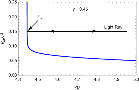
Figure 1 shows the variation of the photon capture radius $r_{\text{ps}}$ on the equatorial plane and the singularity radius $r_{s}$ as functions of $\gamma$. Note that the photon capture radius exists only for $\gamma\geq 1/2$. However, for $\gamma<1/2$, it does not exist as $r_{\text{ps}}<r_{s}$ in this case. This is also clear from the effective potential $V_{\text{eff}}^{\pi/2}$. For $\gamma>1/2$, $V_{\text{eff}}^{\pi/2}$ vanishes both at the singularity $r_{s}$ and at the spatial infinity with a maximum in between marking the position of $r_{\text{ps}}$. However, for $\gamma<1/2$, $V_{\text{eff}}^{\pi/2}$ diverges at the singularity $r_{s}$ (see Fig. 2). Therefore, in this latter case, photons on the equatorial plane will always have turning points outside the singularity. This is also true for off-equatorial photon geodesics. The reason is that, if the geodesics governed by Eq. (16) always have turning points, then so do the ones governed by Eq. (14), as, in the limit $r\to r_{s}$, the effective potential in Eq. (14) still diverges and the coefficient of $\dot{\theta}^{2}$ vanishes. Therefore, in the $\gamma<1/2$ case, as a photon with any non-zero impact parameter always has a turning point, there will be no capturing of photons at all, and hence no shadow will be produced in this case.

To check the above results, we use our numerical ray-tracing techniques (with certain modifications) discussed in our previous work Suvankar_2020 and produce the images. We shoot photons with different impact parameters from a distant observer towards the lensing objects and integrate the geodesic equations backward in time. If a geodesic has a turning point and escapes to infinity for a given impact parameter, we assign bright point to this. On the other hand, if it is captured by the singularity, we assign dark point to the corresponding impact parameter. However, since at the singularity $r_{s}=\frac{2M}{\gamma}$ some of the metric functions become infinite, we cannot exactly touch the surface of singularity due to numerical limitation. We shall have to take a region of tolerance $(\delta r)$ around the singularity. Therefore, we take the inner grid to be at $r=r_{s}+\delta r$, where $\delta r$ is very small. Any photon hitting this surface is assumed to be captured by the singularity. Also, while performing ray-tracing, we consider piecewise step size in the affine parameter $\lambda$. When the radial coordinate reaches below a predefined value $r_{s}+0.3$, i.e., when $r\leq(r_{s}+0.3)$ along a geodesic, we decrease the step size to $\Delta\lambda=10^{-5}$.

Figure 3 shows the ray-traced shadows of the $\gamma$-metric for different $\gamma$. Note that, for $\gamma\geq 1/2$, the singularity always casts shadows whose shapes and sizes will depend on the value of $\gamma$. The shadow becomes more and more prolate as we decrease $\gamma$. This is similar to the results obtained in Bambi_2019; Galtsov_2019. However, for $\gamma=0.4$, we note that the dark region shrinks as we decrease $\delta r$ and will vanish in principle in the limit $\delta r\to 0$. Therefore, as explained before via a theoretical argument, $\gamma<1/2$ case does not cast any shadow. This conclusion is in contradiction to the studies of shadows in Bambi_2019; Galtsov_2019.

The shrinking of the dark region with decreasing $\delta r$ can be understood in more detail from the analysis of geodesics on the equatorial plane. In Fig. 4, we have shown dependence of the impact parameter on turning point $r_{tp}$ for equatorial geodesics. Note that the turning point lies very close to the singularity even when the impact parameter is $\sim$ $3$ or $4$. If we take the turning point to be $r_{tp}=r_{s}+0.001$, then corresponding impact parameters are $2.92$ $2.13$ and $1.15$ for $\gamma=0.45$, $0.4$ and $0.3$, respectively. Therefore, if we take $\delta r=0.001$, then this means that we are excluding all those photons having turning points $r_{tp}\leq(r_{s}+0.001)$, i.e., from the impact parameters space, we are excluding impact parameters $b\leq 2.92$, $2.13$ and $1.15$ for $\gamma=0.45$, $0.4$ and $0.3$, respectively. Photons having impact parameters within the excluded region form dark spots. As a result, we are having the dark region for $\gamma<1/2$. However, for a given $\gamma<1/2$, decreasing $\delta r$ means decreasing the excluded region from the impact parameter space. The excluded region and hence the dark region vanishes in the limit $\delta r\to 0$. Therefore, we do not have any shadow in principle in the $\gamma<1/2$ case.

We now use the results from M87^∗ observation (EHT1) and put possible constraint on the $\gamma$-metric. For this purpose, we use the average size of the shadow and its deformation from circularity. To this end, we first denote the horizontal and the vertical axes in the shadow plane by $\alpha$ and $\beta$ respectively and define an angle $\phi$ between the $\alpha$-axis and the vector connecting the geometric centre $(0,0)$ of the shadow with a point $(\alpha,\beta)$ on the boundary of a shadow. Therefore, the average radius $R_{av}$ of the shadow is given by (Bambi)

where $l(\phi)=\sqrt{\alpha(\phi)^{2}+\beta(\phi)^{2}}$ and $\phi=tan^{-1}(\beta(\phi)/\alpha(\phi))$. Following EHT1, we define the deviation $\Delta C$ from circularity as

Note that $\Delta C$ is the fractional RMS distance from the average radius of the shadow.

According to EHT collaboration, the angular size of the observed shadow is $\Delta\theta_{sh}=42\pm 3$ $\mu$as, and its deviation from circularity ($\Delta C$) is less than $10\%$ (EHT1). Also, following EHT1, we take the distance to M87^∗ to be $D=(16.8\pm 0.8)$ Mpc and the mass of the object to be $M=(6.5\pm 0.7)\times 10^{9}M_{\odot}$. These numbers imply that the diameter of the shadow in dimensionless unit should be

where the errors have been added in quadrature. The above quantity must be equal to $\frac{2R_{av}}{M}$, i.e., $\frac{d_{sh}}{M}=\frac{2R_{av}}{M}$. In Fig. 5, we have shown the average diameter and the deviation from circularity of the shadow for different $\gamma$ and the observers inclination angle $\theta_{o}$. Here, we have taken $0.5\leq\gamma\leq 1$. Note that the size of the shadow is consistent with the M87^∗ observations for all $\gamma$ and $\theta_{o}$. However, the deviation from circularity is more than $10\%$, i.e., $\Delta C>0.1$ over a small parameter region where $\gamma$ is close to $0.5$ and inclination is high simultaneously. If we restrict the inclination angle to be $\theta_{o}=17^{\circ}$, which the jet axis makes to the line of sight (EHT1), then both the shadow size and the deviation from circularity are consistent with the M87^∗ observations for all $\gamma$ values considered in Fig. 5. For the $\gamma>1$, we have found that both the size and the deviation from circularity slowly increases with increasing $\gamma$ for a given inclination angle. Therefore, in this latter case, the maximum size and deviation occur for the GI spacetime. We have found that, for $\theta_{o}=17^{\circ}$ and $\gamma>1$, these maximum values are given by $d_{sh}/M\simeq 10.46$ and $\Delta C\simeq 0.028$, which are consistent with the observation. Therefore, we find that, for the inclination angle of $17^{\circ}$, the shadow of the $\gamma$-metric is always consistent with the M87^∗ observations for all $\gamma\geq 1/2$.

We now consider the properties and image of a geometrically thin accretion disk in the $\gamma$-metric given in Eq. (2). The disk consists of massive particles moving in stable circular timelike geodesics¹¹ 1 Strictly speaking, the particles move on almost circular geodesics and are very slowly infalling on the equatorial ($\theta=\pi/2$) plane and is described by the Novikov-Thorne model (novikov_1973; page_1974). Since the spacetime has time translational and azimuthal symmetries, we have two constants of motion along a timelike geodesic, namely, the specific energy $\tilde{E}$ (energy per unit mass) and the specific angular momentum $\tilde{L}$ about the axis of symmetry respectively. Therefore, the geodesic equations corresponding to $t$ and $\phi$ can be written as,

From the normalization of four velocity $u^{\mu}$ (i.e. $u^{\mu}u_{\mu}=-1$) for massive particles, the radial geodesic equation on the equatorial plane can be written as

where $\tilde{V}_{eff}$ is the effective potential. A stable circular orbit is given by $\tilde{V}_{\text{eff}}=0$, $\tilde{V}^{\prime}_{\text{eff}}=0$ and $\tilde{V}_{\text{eff}}^{\prime\prime}<0$. The first two conditions yield the following expressions for the specific energy and the specific angular momentum of the particles moving in the stable circular orbits:

where $\Omega=d\phi/dt$ is the angular velocity of the particles forming the disk. The flux of the electromagnetic radiation emitted from a radial position $r$ of the disk is given by the standard formula (novikov_1973; page_1974)

where $\dot{M}=dM/dt$ is the mass accretion rate, $r_{in}$ is the inner edge of the disk, and $\sqrt{-g}=\sqrt{-g_{tt}g_{rr}g_{\phi\phi}}$ is the determinant of the metric on the equatorial plane. The marginally stable circular orbit is given by $V_{\text{eff}}^{\prime\prime}=0$. This gives

Figure 6 shows the variations of $r_{\pm}$, the radius of singularity $r_{s}=\frac{2M}{\gamma}$ and the photon capture radius $r_{ps}$ as functions of $\gamma$. For $0<\gamma<1/\sqrt{5}$, $r_{\pm}$ do not exist. Therefore, in this case, we have a single continuous disk with its inner edge at $r_{in}=r_{s}$ and outer edge at some radius $r>r_{s}$. For $\gamma=1/\sqrt{5}$, $r_{-}=r_{+}$, i.e., the outer edge of the inner disk coincides with the inner edge of the outer disk, thereby giving a single continuous disk. For $1/\sqrt{5}<\gamma<1/2$, $r_{s}<r_{-}<r_{+}$, implying that there exist stable circular orbits in between the singularity $r_{s}$ and $r_{-}$, and also at radii greater than $r_{+}$ with no stable circular orbits in between $r_{-}$ and $r_{+}$. Therefore, in this case, we have double disk configuration (two concentric disjoint disks). The inner disk extends from the singularity (i.e., $r_{in}=r_{s}$) to $r_{-}$, and the outer disk extends from $r_{in}=r_{+}$ to some radius $r>r_{+}$. For $1/2\leq\gamma\leq 1$, $r_{-}\leq r_{s}<r_{+}$. Therefore, in this case, $r_{-}$ does not exist, and we have a single accretion disk with its inner edge at $r_{in}=r_{+}$ and the outer edge at some radius $r>r_{+}$. Although both the roots $r_{\pm}$ are real for $\gamma>1$ case, the angular momentum $\tilde{L}$ of circular orbits with radii $r\leq r_{-}$ becomes imaginary. Therefore, in $\gamma>1$ case, we have a single disk with its inner edge at $r_{in}=r_{+}$. Note that, in the limit $\gamma\to\infty$, i.e., for the GI spacetime, $r_{s}=0$ and $r_{\pm}=(3\pm\sqrt{5})M$.

We now use our numerical ray-tracing techniques (with certain modifications) discussed in our previous work Suvankar_2020 (see also rajibul_disk) and produce the images of accretion disks. The intensity maps of the images of accretion disks for the different cases discussed above are shown in Fig. 7. Note that, when there are light rings in the $\gamma$-metric, the image is very similar to that of a black hole, thereby mimicking a black hole. In the absence of light rings, however, the images for the $\gamma$-metric differ strikingly from that of the black hole, as shown by Figs. 7(d), 7(e) and 7(f).

The unprecedented advances in observational studies in the current era of the EHT have resulted in the exciting possibility of understanding the nature of singularities in GR, by comparing theory with experimental data. Motivated by the celebrated work of Hawking Hawking, the importance of such studies lies in the fact that these can ultimately throw light on the nature of strong gravity, effective at horizon scales Giddings. An important aspect of such analyses is the fact that one can use the EHT data to constrain possible solutions of Einstein equations. Indeed, a plethora of activities have been reported in this direction in the recent past, and it is by now understood that several singular solutions, as well as horizonless compact objects are consistent with current data. The totality of such results will be pivotal in understanding the correct nature of the fundamental aspects of strong gravity.

In this paper, we have carried out the analysis of shadows and accretion disk images of the Zipoy-Voorhees spacetime, characterized by the $\gamma$-metric. We have shown that while for the parameter $\gamma<1/2$, there will be no shadow, the $\gamma\geq 1/2$ class is essentially unconstrained, i.e., all such values of $\gamma$ are consistent with current EHT observations. We have further constructed thin accretion disk images in the $\gamma$ metric background and shown that these can be dramatically different from the Schwarzschild case for $\gamma<1/2$.

As we mentioned in the introduction, astrophysical black holes are often approximated by the static Schwarzschild or the stationary Kerr solution. The $\gamma$-metric on the other hand describes a static, axially-symmetric vacuum solution, and is attractive in its own rights. Since spherical symmetry in static vacuum solutions is by no means a fundamental criterion in black hole physics, our result that the $\gamma$-metric is perfectly admissible, should be an interesting addition to the current literature. Further, we have shown how the thin accretion disk images here might be very similar to that of the Schwarzschild black hole in cases when there are light rings. These cases thus exemplify situations where the horizonless object might mimic a black hole. In the absence of any light ring, however, these images might be very different from the black hole case.

In continuation of this work, it should be interesting to compare other static axially symmetric solutions of GR with the current data from the EHT.

References

- (1) The Event Horizon Telescope Collaboration, First M87 event horizon telescope results. I. The shadow of the supermassive black hole, Astrophys. J. Lett. 875, L1 (2019).
- (2) The Event Horizon Telescope Collaboration, First M87 event horizon telescope results. V. Physical origin of the asymmetric ring, Astrophys. J. Lett. 875, L5 (2019).
- (3) The Event Horizon Telescope Collaboration, First M87 event horizon telescope results. VI. The shadow and mass of the central black hole, Astrophys. J. Lett. 875, L6 (2019).
- (4) R. Shaikh, K. Pal, K. Pal and T. Sarkar, Constraining alternatives to the Kerr black hole, arXiv:2102.04299 [gr-qc].
- (5) D. Psaltis et al. (Event Horizon Telescope), Gravitational Test Beyond the First Post-Newtonian Order with the Shadow of the M87 Black Hole, Phys. Rev. Lett. 125, 141104 (2020).
- (6) I. Banerjee, S. Chakraborty and S. SenGupta, Silhouette of M87*: A New Window to Peek into the World of Hidden Dimensions, Phys. Rev. D 101, no. 4, 041301 (2020).
- (7) C. Bambi, K. Freese, S. Vagnozzi and L. Visinelli, Testing the rotational nature of the supermassive object M87∗ from the circularity and size of its first image, Phys. Rev. D 100, 044057 (2019).
- (8) R. Kumar and S. G. Ghosh, Black Hole Parameter Estimation from Its Shadow, ApJ 892, 78 (2020).
- (9) G. Erez and N. Rosen, The gravitational field of a particle possessing a multipole moment, Bull. Res. Council Israel 8, 47 (1959).
- (10) D. M. Zipoy, Topology of some spheroidal metrics, J. Math. Phys. 7, 1137 (1966).
- (11) B. H. Voorhees, Static axially symmetric gravitational fields, Phys. Rev. D 2 2119 (1970).
- (12) F. P. Esposito, L. Witten, On a static axisymmetric solution of the Einstein equations, Phys. Lett. B58, 357 (1975).
- (13) Ts. I. Gutsunaev, V. S. Manko, On the Gravitational Field of a Mass Possessing a Multipole Moment, Gen. Rel. Grav. 17 1025 (1985),
- (14) H. Stephani, D. Kramer, M. Maccallum, C. Hoenselaers, E. Herlt, Exact Solutions to Einstein’s Field Equations 2 Ed., Cambridge University Press (2003).
- (15) J. B. Griffiths and J. Podolsky, Exact Space-Times in Einstein’s General Relativity, Cambridge University Press, Cambridge, United Kingdom, 2009.
- (16) L. Herrera, F. M. Paiva, N. O. Santos, The Levi-Civita space–time as a limiting case of the space–time, J. Math. Phys. 40, 4064 (1999).
- (17) H. Kodama and W. Hikida, Global structure of the Zipoy-Voorhees-Weyl spacetime and the delta=2 Tomimatsu-Sato spacetime, Classical and Quantum Gravity 20, 5121 (2003).
- (18) D. V. Gal’tsov, K. V. Kobialko, Photon trapping in static axially symmetric spacetime, Phys. Rev. D 100 104005 (2019).
- (19) A. B. Abdikamalov, A. A. Abdujabbarov, D. Ayzenberg, D. Malafarina, C. Bambi, and B. Ahmedov, A black hole mimicker hiding in the shadow: Optical properties of the -metric, Phys. Rev. D 100, 024014 (2019).
- (20) L. Herrera, G. Magli and D. Malafarina, “Non-spherical sources of static gravitational fields: Investigating the boundaries of the no-hair theorem,” Gen. Rel. Grav. 37, 1371 (2005)
- (21) K. S. Virbhadra, Directional naked singularity in general relativity, arXiv:gr-qc/9606004.
- (22) K. Boshkayev, E. Gasperin, A. C. Gutierrez-Pineres, H. Quevedo, and S. Toktarbay, Motion of test particles in the field of a naked singularity, Phys. Rev. D 93, 024024 (2016).
- (23) H. Quevedo, Mass quadrupole as a source of naked singularities, Int. J. Mod. Phys. D 20, 1779 (2011).
- (24) J. L. Hernández-Pastora and J. Martín, Monopole-Quadrupole Static Axisymmetric Solutions of Einstein Field Equations, Gen. Rel. and Grav. 26, 877 (1994).
- (25) A. N. Chowdhury, M. Patil, D. Malafarina, and P. S. Joshi, Circular geodesics and accretion disks in the Janis-Newman-Winicour and gamma metric spacetimes, Phys. Rev. D 85, 104031 (2012).
- (26) J. Chazy, Sur la champ de gravitation de deux masses fixes dans la theory de la relativit’e, Bull. Soc. Math. Fr. 52, 17 (1924).
- (27) H. E. J. Curzon, Cylindrical solutions of Einstein’s gravitation equations, Proc. London Math. Soc. 23, 477 (1924).
- (28) P. M. Camacho, F. F. Alfaro, and C. G. Chaves, Slowly rotating Curzon-Chazy metric, Rev. Mat. Teor. Apl. 22, 265 (2015).
- (29) S. Paul, R. Shaikh, P. Banerjee and T. Sarkar, Observational signatures of wormholes with thin accretion disks, JCAP 03 (2020) 055.
- (30) I. D. Novikov and K. S. Thorne, Astrophysics and black holes, in Black Holes, edited by C. DeWitt and B. DeWitt (Gordon and Breach, New York, 1973).
- (31) D. N. Page and K. S. Thorne, Disk-accretion onto a black hole. Time-averaged structure of accretion disk, Astrophys. J. 191, 499 (1974).
- (32) R. Shaikh and P. S. Joshi, Can we distinguish black holes from naked singularities by the images of their accretion disks?, JCAP 10 (2019) 064.
- (33) S. W. Hawking, Particle Creation by Black Holes, Commun. Math. Phys. 43, 199 (1975) Erratum: [Commun. Math. Phys. 46, 206 (1976)].
- (34) S. B. Giddings, Searching for quantum black hole structure with the Event Horizon Telescope, Universe 5, no. 9, 201 (2019)