TNet: A Model-Constrained Tikhonov Network Approach for Inverse ProblemsThanks: The first version of work was an Oden Institute technical report 21-09, May 11, 2021, and then presented at the Uncertainty Quantification and Probabilistic Modeling Technical Thrust Area, USNCCM, May 17, 2021.
Abstract
Deep Learning (DL), in particular deep neural networks (DNN), by default is purely data-driven and in general does not require physics. This is the strength of DL but also one of its key limitations when applied to science and engineering problems in which underlying physical properties—such as stability, conservation, and positivity—and desired accuracy need to be achieved. DL methods in their original forms are not capable of respecting the underlying mathematical models or achieving desired accuracy even in big-data regimes. On the other hand, many data-driven science and engineering problems, such as inverse problems, typically have limited experimental or observational data, and DL would overfit the data in this case. Leveraging information encoded in the underlying mathematical models, we argue, not only compensates missing information in low data regimes but also provides opportunities to equip DL methods with the underlying physics, and hence promoting better generalization. This paper develops a model-constrained deep learning approach and its variant TNet—a Tikhonov neural network—that are capable of learning not only information hidden in the training data but also in the underlying mathematical models to solve inverse problems governed by partial differential equations. We provide the constructions and some theoretical results for the proposed approaches. We show that data randomization can enhance not only the smoothness of the networks but also their generalizations. Comprehensive numerical results not only confirm the theoretical findings but also show that with even as little as training data samples for 1D deconvolution, for inverse 2D heat conductivity problem, for inverse initial conditions for time-dependent 2D Burgers’ equation, and for inverse initial conditions for 2D Navier-Stokes equations, TNet solutions can be as accurate as Tikhonov solutions while being several orders of magnitude faster. This is possible owing to the model-constrained term, replications, and randomization.
keywords
Inverse problem, randomization, model-constrained, deep learning, deep neural network, partial differential equations.1 Introduction
Inverse problems are pervasive in scientific discovery and decision-making for complex, natural, engineered, and societal systems. They are perhaps the most popular mathematical approaches for enabling predictive scientific simulations that integrate observational/experimental data, simulations and/or models [46, 28, 62]. Many engineering and science systems are governed by parametrized partial differential equations (PDE). Computational PDE-constrained inverse problems face not only the ill-posed nature—namely, non-existence, non-uniqueness, and instability of inverse solutions—but also the computational expense of solving the underlying PDEs. Computational inverse methods typically require the PDEs to be solved at many realizations of parameter and the cost is an (possibly exponentially) increasing function of the parameter dimension. The fast growth of this cost is typically associated with the curse of dimensionality. Inverse problems for practical complex systems [3, 46, 31, 12, 32] however possess this high dimensional parameter space challenge. Thus, mitigating the cost of repeatedly solving the underlying PDE has been of paramount importance in computational PDE-constrained inverse problems.
The field of Machine Learning (ML) typically refers to computational and statistical methods for the automated detection of meaningful patterns in data [7, 57, 41]. While Deep Learning (DL) [22], a subset of machine learning, has proved to be state-of-the-art methods in many fields of computer sciences such as computer vision, speech recognition, natural language processing, etc, and its presence in the scientific computing community is, however, mostly limited to off-the-shelf applications of deep learning. Unlike classical scientific computational methods, such as finite element methods [15, 10, 18], in which solution accuracy and reliability are guaranteed under regularity conditions, standard DL methods are often far from providing reliable and accurate predictions for science and engineering applications. The reason is that though the approximation capability of deep learning, e.g. via Deep Neural Networks (DNN), is as good as classical methods in approximation theory [17, 24, 38, 27], DL accuracy is hardly attainable in general due to limitation in training. It has been shown that the training problem is highly nonlinear and non-convex, and that the gradient of loss functions can explode or vanish [23], thus possibly preventing any gradient-based optimization methods from reliably converging to a minimizer. Even when converged, the prediction of the (approximate) optimal deep learning model can be prone to over-fitting and can have poor generalization error.
Many data-driven inverse problems in science and engineering problems have limited experimental or observational data, e.g. due to the cost of placing sensors (e.g. digging an oil well can cost million of dollars) or the difficulties of placing sensors in certain regions (e.g. deep ocean bottoms). DL, by design, does not require physics, but data. This is the strength of DL. It is also the key limitation to science and engineering problems in which underlying physics needs to be respected and higher accuracy is required. In this case, purely data-based DL approaches are prone to over-fitting and thus incapable of respecting the physics or providing the desired accuracy. Similar to least squares finite element methods [8], we can train a DNN solution constrained by the PDE residual as a regularization [56, 52, 54, 55, 67, 64, 36, 48]). Such an approach attempts to learn an approximate solution by making the -norm of PDE residual small. While universal approximation results (see, e.g., [17, 24, 38, 27, 11]) could ensure any desired accuracy with a sufficiently large number of neurons, practical network architectures are moderate in both depth and width, and hence the number of weights and biases. Therefore, the accuracy of learning PDE solutions in function spaces can be limited.
We are interested in parametrized PDEs—that are pervasive in design, control, optimization, inference, and uncertainty quantification. Attempts using pure data-driven deep learning to learn the parameter to observable map have been explored (see, e.g., [30, 66, 49, 61, 50, 30, 59, 25, 58]). Approaches using autoencoder spirit that train a forward network first and then an inverse network in tandem [35, 40] or both of them simultaneously [21] have also been proposed. The work in [68] proposes to use a graph neural network to approximate forward solver and and fully connected neural network to learn a regularization via the prior knowledge. Once trained, both networks are deployed in a Tikhonov-like regularization algorithm to obtain the inverse solution. While successes are reported, generalization capability, and hence success, could be limited to regimes seen in the training data as the governing equations—containing most, if not all, information about the underlying physics—are not involved in the training.
In order to take into account the underlying problem, a natural direction is to deploy deep learning methods as surrogates for expensive or difficult components in traditional methods. Such a hybrid approach can enjoy the benefits of both sides. For example, learning regularizers to penalize certain undesirable features has been proposed for both inverse [33, 39] and imaging [2] problems. Once trained, these regularizers can be used in any traditional inverse or imaging methods. The main disadvantage of these approaches is that they may still experience the same computational expense as traditional methods when the forward map is the most expensive part. Learning the forward map [34, 68, 4, 51] is thus desirable, though it may not be considered as a model-aware approach.
A logical alternative is thus to constrain the learning of inverse solution with the underlying governing equations and/or physics. The work in [1] proposes to partially learn the gradient of a Tikhonov functional and uses the learned gradient to perform a gradient-based optimization method for solving imaging problems. A natural extension of the physics-informed neural network framework [14, 53, 36, 37] is to train two networks, one for solutions and another for unknown parameters. In an attempt to mimic the traditional PDE-constrained approach, [19, 6] parametrize the unknown parameters using feed-forward neural networks whose weights/biases are then found by an optimization approach constrained by the Navier-Stokes equations and heat equations. These methods, however, may not be efficient as new observational data (corresponding to new unknown parameters) requires retraining. It is also not clear how to extend them to statistical inverse problems.
Learning inverse maps constrained by the underlying governing equations has also been investigated. The work in [47], similar to [19, 6], presents an autoencoder-like approach in which the encoder is the inverse map and the decoder is the numerical solutions of the underlying governing equations evaluated at observational points. The network weights/biases are found by minimizing the data misfit. Taking both the data misfit and the regularization into account as in the traditional Tikhonov inversion approach, [26] solves 1D seismic inversion methods with promising results. The beauty of this approach is that, once trained, the neural network can be deployed to approximately solve inverse problems in real-time.
The main contributions of this paper—a detailed extension of an approach set forth in a more general framework in [44]—is as follows. Unlike similar and independent work in [47, 19, 6, 26], our mcDNN has a theoretical foundation, from which and numerical evidence, we infer that mcDNN may not be a good learning strategy for inverse problems as it could be biased by the training data, though it is interpretable compared to a purely data-driven counterpart. This motivates us to develop a new model-constrained deep learning approach, called TNet, designed to learn the Tikhonov inverse solution, and indeed it recovers Tikhonov regularized solutions for linear inverse problems. We also propose to randomize the training data and rigorously justify randomization as an implicit regularization that could improve the generalization of the proposed deep-learning approaches. We provide comprehensive numerical results to support our developments for 1D deconvolution, inverse heat conductivity, and inverse initial conditions for both time-dependent 2D Burgers’ and 2D Navier-Stokes equations.
The paper is organized as follows. In section 2 we introduce nonlinear inverse problems, and a data-driven naive DNN (nDNN) approach. The goal of section 3 is to present a model-constrained DNN (mcDNN) approach designed to learn the inverse map while being constrained by the parameter-to-observable map of the underlying discretized PDE. Though mcDNN is interpretable, it could be biased toward training data. This leads us to develop TNet—a Tikhonov neural network—in section 4 that aims to learn the Tikhonov solver while removing unnecessary biases. We show that data randomization can make TNet not only more robust but also generalize better: thanks to the model-constrained training. In section 5 and the supplementary document, comprehensive numerical results supporting our developments are presented for 1D deconvolution, inverse heat conductivity, and inverse initial conditions for both time-dependent 2D Burgers’ and 2D Navier-Stokes equations. We conclude the paper with future research directions in section 6. Proofs of the theoretical results, practical implementation aspects of our proposed approaches, and specifications of trainings are provided in the supplementary document.
2 Introduction to forward and inverse problems
The following notations are used in the paper. Boldface lowercases are reserved for (column) vectors, and uppercase letters are for matrices. We denote by the parameters sought in the inversion or the parameter of interest (PoI), by the forward states, by the forward map (computing some observable quantity of interest), and by the observations given by
| (1) |
where is some additive observation noise. The parameter-to-observable (PtO) map is the composition of the forward map and the states, i.e., . However for simplicity of the exposition, we do not distinguish it from the forward map and thus we also write . The forward state is the solution of the forward equation
| (2) |
Assume that eq. 2 is well-posed so that, for a given set of parameters , one can (numerically for example) solve for the corresponding forward states . In the forward problem, we compute observational data via eq. 1 given a set of parameter . In the inverse problem, we seek to determine the unknown parameter given some observational data , that is, we wish to construct the inverse of . Since is typically (much) larger than for many practical problems, the parameter-to-observable map is not invertible even when is linear. The inverse task is thus ill-posed and notoriously challenging as a solution for may not exist, even when it may, it is not unique nor stably depends on the data . An approximate solution is typically sought via (either deterministic or statistical) regularization.
Given the popularity of emerging machine learning, in particular deep neural networks (DNN), methods, we may attempt to apply a naive pure data-driven DNN (nDNN) to learn the (ill-posed) inverse of , e.g.,
| (nDNN) |
where is a DNN with weight matrix and bias vector and the last two terms are regularizations for weights and biases with nonnegative regularization parameters and . Here, is the data matrix concatenating observational data , , and is the parameter matrix concatenating the corresponding parameter vectors . This approach completely disregards the underlying mathematical model eq. 1-eq. 2. Even for linear inverse problem—for example, and there is no error in computing the data so that —and linear DNN such as , where , and thus the optimal weight and bias for eq. nDNN are given as
where and denotes the pseudo-inverse operation, it is not clear if the nDNN inverse solution
provides an approximate solution to the original inverse problem
in an interpretable sense. This is a disadvantage of pure data-driven approaches.
The data-driven nature of DNN could be claimed as an advantage. However, DNN can be considered as an “interpolation” method and thus can generalize well only for scenarios that have been seen in or are sufficiently close to the training data set . This implies a possible enormous amount of training data to learn the inverse of highly non-linear problems. In practical sciences and engineering problems, this extensive data regime is unfortunately rarely the case due to the high cost of placing sensors or the difficulties in placing sensors in certain regions. In order for a DNN to generalize well in insufficient/low data regimes, it should be equipped with information encoded in the forward model eq. 1-eq. 2 that is not covered in the data set. Such a physics encoding also supplies meaningful interpretations to DNN inverse solutions as we shall show. The question is how to inform DNN about the underlying models? In the following, we construct two DNNs to learn the inverse of the PtO map not only by information hidden in the training data but also by satisfying the forward equations exactly at the training points.
3 Model-Constrained Deep Neural Network (mcDNN) for learning the inverse map
We propose to learn the inverse map via DNN constrained by the forward map as
| (mcDNN) |
where is a DNN learning the map from observable data to parameter with weight matrix and bias vector . We have introduced Frobenius norm weighted by in the first term as
and similarly for the second term weighted by . Unlike the naive purely data-driven DNN approach eq. nDNN, the model-constrained eq. mcDNN makes the DNN aware that the training data is generated by the forward map . This is done by requiring the output of the DNN—approximate unknown parameter for a given data as the input—when pushed through the forward model , reproduces the data . The model-aware term can be considered as a physics-aware regularization approach for mcDNN (compared to the non-physical regularizations in eq. nDNN). The architecture of mcDNN is presented in fig. 1.
In order to shed light on our mcDNN approach let us choose a linear activation function such that the one-layer DNN model for leaning the inverse map can be written as , where . We also assume that the forward map is linear. For linear inverse problem with linear DNN, the model-constrained training problem eq. mcDNN becomes
| (3) |
Lemma 1.
The optimal solution and of the DNN training problem eq. 3 satisfies
where and are the column-average of the training parameters and data, , and .
Corollary 2 (mcDNN is a Tikhonov solver).
For a given testing/observational data , the mcDNN inverse solution of eq. 3 is given by
which is exactly the solution of the following Tikhonov regularized linear inverse problem
where
| (4) |
The results of corollary 2 shows that the mcDNN inverse solution is equivalent to a Tikhonov-regularized inverse solution with a data-informed reference parameter that depends on the training set and the given observational data . In other words, the model-constrained deep learning mcDNN approach is interpretable in the sense that it provides data-informed Tikhonov-regularized inverse solutions.
4 Tikhonov neural network (TNet) for learning the inverse map
We observe that the reference parameter in corollary 2 depends on the training data, and thus the model generalization depends on the amount of training data. In other words, mcDNN solution could have a strong bias to the training data and may limit the generalization which is not desirable especially for scenarios that are not very close to the training ones. On the other hand, in the classical Tikhonov regularization framework, the reference parameter is fixed and independent of the observable data. From a statistical point of view, the reference parameter is typically the mean of the prior distribution of the parameter of interest (PoI) , which reflects the a priori belief on how the PoI should look like on average. Synergizing mcDNN and Tikhonov regularization ideas, we propose a Tikhonov neural network TNet—a semi-supervised model-constrained learning approach—where, unlike mcDNN, the unknown PoI predicted by the DNN are forced to be close the PoI prior mean as
| (TNet) |
where is the matrix whose columns are the mean prior of the PoI. Consequently, the architecture of TNet is the same as mcDNN in fig. 1 except with replaced by . Applying corollary 2 to TNet for linear inverse problem with linear DNN we have the following result.
Corollary 3 (TNet is a Tikhonov solver).
For a given testing/observational data , the TNet inverse solution is given by
| (5) |
which is exactly the solution to the following Tikhonov regularized linear inverse problem
where
Two observations are in order. First, corollary 3 shows that the TNet inverse solution is exactly the Tikhonov-regularized inverse solution with the true prior mean as the reference parameter provided that the observation data is full row rank. This holds, for example, when the number of independent data is at least the same as the number of observations. Even when this happens, mcDNN solution in corollary 2 does not coincide with the Tikhonov solution as the first two terms on the right-hand side of eq. 4 only reduce to in the limit of infinite training data (via the law of large numbers). Second, training data for PoI is not needed (thanks to the semi-supervised learning nature of TNet). This is particularly useful when we like to use actual observational data in training.
The next result is a highlight of our method in that our model-constrained approaches satisfy the governing equation exactly at the training points. The proof and aspects on practical implementation are provided in section 7 and section 8.
Proposition 4 (Exactly satisfying the governing equations at training points).
Both mcDNN and TNet inverse solutions satisfy the governing equations exactly at all training points.
We now show that data randomization enhances not only the generalization of TNet solution but also its robustness to observational noise. To begin, we randomize a generic data vector , e.g. one column of , as follows
| (6) |
where a Gaussian noise vector with variances is added to the data. We emphasize that the following arguments also hold for any random noise vector with independent components, each of which is a random variable with zero mean and variances . Let denote the expectation with respect to . Following [5], for a generic loss function , we perform the Taylor expansion around up to second order to obtain
| (7) |
where we have used sufficient small noise variance so that the high-order term , using the standard “small o” notation, is negligible.
For training data set with samples, we randomize each sample as , where . Note that we can use different noise levels for data randomization. In that case, the eq. TNet loss becomes
| (8) |
Replacing with in eq. 7 yields
| (9) |
where
| (10) |
and the induced penalty terms are given by
in which is the trace operator, and denotes the dot product of a third-order tensor and a vector. It can be observed that the training loss with randomized data is the sum of the original loss plus four induced regularization terms. is non-negative and promotes the smoothness of the neural network. The second term of eq. 10 ensures that is close to the right inverse of , and strengthen this closeness by forcing the derivative of the to the identity. These two effects together behave like a Hermite interpolation in which not only the function values but also the derivatives are required to be matched closely at the training points. The two terms in eq. 10 make and necessary small, and as a result, and can be dominated by and , respectively. It is interesting to see that and can encourage the second derivatives (and hence extra smoothness) of the neural network and to be small. In other words, the beauty of data randomization is that it can promote a -Sobolev-like Tikhonov regularization for the neural network via eq. 10, , and . Moreover, it can further enforce to be the same as the right inverse of the PtO map up to second derivatives via eq. 10, , and .
Accounting for the data randomization for all training data we can—after taking the expectation with the random noise , —write eq. 8 as
| (11) |
Thus, on average, the TNet loss with randomized data is approximately the sum of the original TNet loss (without randomization) plus four regularization terms for each training data point. These induced regularization terms play a vital role in stimulating the robustness and accuracy of the neural network. Indeed, without data randomization, the TNet loss eq. TNet simply requires the neural network outputs to be close to the parameter data via the data misfit (the first) term, and the neural network, when pushed through the PtO map, resembles the observational data via the model-constrained (the second) term. Whereas, randomizing the data enforces not only the smoothness of the neural network up to second order derivative (through the first term) but also the agreement of the neural network and the right inverse of the PtO map up to second order derivatives (through the model-constrained term). Let us summarize the above result in the following theorem.
Theorem 5.
Let , where . Then
| (12) |
Remark 6.
Note that are not necessarily different from each other. However, the Hermite interpolation analogy tells us that we should have as many distinct baseline training points as possible for good generalization. It turns out that we just need a small number of distinct training points to have accurate results, as numerically shown in section 5. The above randomization approach also holds for nDNN and mcDNN approaches. Indeed, in the the final expression eq. 11 we simply replace by (see eq. mcDNN) and by in for mcDNN. Similarly for nDNN, we replace by (see eq. nDNN) and remove and .
5 Numerical results
Noise realization. For all numerical results, we choose for all in eq. 12, where denotes the relative noise level.
Data generation and training. For non-linear problems in section 5.1, section 10.2 and section 5.2, we use a shallow neural network having one hidden layer with 5000 ReLU neurons. We verified that a dense feed-forward neural network architecture with multiple layers could provide comparable results but with large training data sets. In small data regimes, i.e. 100 samples, deep networks perform poorly due to the vanishing gradient problem and/or the bias-variance trade-off problem. Moreover, training a deep learning network faces further challenges [20, 60] that are beyond the scope of this paper. We thus focus on neural networks with a single hidden layer and this is sufficient to demonstrate the proposed TNet framework. Regarding optimization algorithm, the default ADAM [29] optimizer in JAX [9] is used. In all numerical results, weights and biases of the neural network are initialized by standard Gaussian distribution and a zero vector, respectively, using the same random seed. Therefore, we begin the training process with the same network for all cases.
In order to be fair, within any comparison we use the same random seeds for noise. To ensure that more training data can offer more information, the training data set is generated in a nested manner, e.g., , and so on, where denotes the number of training samples. For any testing, except for the linear deconvolution problem in which we use testing samples, a test data set of 500 samples is used to compare approaches. The Tikhonov inverse solutions are obtained by the default BFGS algorithm [45] in Jax [9]. A summary of training parameters is presented in table 6 in the supplementary.
Accuracy metric. To estimate the accuracy of each approach, we compute average relative errors from unseen random samples: the first based on pointwise values and the second on Euclidean norm of the inverse parameter vector as follows
| (13) |
and
| (14) |
where superscript denotes the th sample, subscript denotes the th component of the vector under consideration, and is the number of spatial grid points. Here, “pred” stands for the solution predicted by the neural network, and “true” for the synthetic ground truth parameters.
5.1 2D heat conductivity inverse problem
The heat equation we consider is the following
where the conductivity is the parameter of interest (PoI), is the temperature field, and n is the unit outward normal vector on Neumann boundary part . fig. 2 shows the domain (left subfigure) and a mesh (right subfigure) together with the locations of 10 observational points of the state . In this problem, we are interested in reconstructing the PoI field given a set of 10 pointwise observations.
Generating train and test data sets. We start with drawing the parameter conductivity samples via a truncated Karhunen-Loéve expansion
where is the eigenpair of a two-point correlation function from [16], and is a standard Gaussian random vector. We choose eigenvectors corresponding to the first largest eigenvalues. For each sample, we discretize initial vorticity , denoted as , and we solve the heat equation for the temperature by finite element method. Observations are obtained by extracting values of the temperature field at observational points, which are then corrupted with additive Gaussian noise with a noise level of . A pair of conductivity field and its corresponding temperature distribution is depicted in the middle column of fig. 15. We generate test pairs using the same process.

Next, we consider two cases of train data for learning the inverse map from observations to conductivity. Case I: Full base, i.e., distinct training samples are used; and Case II: we first pick a number of distinct baseline samples smaller than , and then replicate and randomize them to obtain samples for the train data set. For each case, the average relative error in eq. 14 is computed with 500 true test samples for nDNN, mcDNN and TNet, and is compared to the relative error of the Tikhonov regularization approach.
Case I: Training with full data sets . We train nDNN, mcDNN and TNet networks using three different full training data bases, and present the smallest errors in table 1. As can be seen, larger data sets provide more accurate inverse maps. In particular, the average smallest relative errors for nDNN for these training sets are 60.41%, 50.69% and 49.07% which are higher than 57.27%, 50.39% and 48.40%, respectively, for mcDNN. With the smallest errors of 45.98%, 45.35% and, 44.98%, correspondingly, TNet outperforms nDNN and mcDNN by a significant margin, and is similar to Tikhonov (TIK) approach. It is not surprising since TNet approach is designed to learn Tikhonov method, as discussed in section 4. This is further confirmed by the fact that while regularization parameters for mcDNN, TNet, and Tikhonov approaches are the same, namely , only TNet and Tikhonov solutions agree well with each other for a wide range of regularization parameters, as shown in fig. 3. On the contrary, a data-driven approach such as nDNN requires sufficient training data (more than 100 for this case as fig. 3 indicates) to provide a reasonable solution. We note that mcDNN is not much more accurate than nDNN for this example, perhaps due to strong bias from the data as suggested by corollary 2.
The preceding discussion also alludes to an important point. In particular, identifying a good approximation of the optimal regularization parameter plays a vital part in TNet performance. This can be accomplished by finding a good regularization parameter for the Tikhonov approach and using it for TNet. The subject of determining a suitable regularization parameter has been studied extensively in the literature using various approaches including the Morozov discrepancy principle, L-curve, and cross-validation [42, 63, 65]. The numerical results in fig. 3 show that TNet and mcDNN results are robust in accuracy for a sufficiently large neighborhood around the optimal Tikhonov regularization parameter, and thus a reasonable regularization parameter is sufficient for TNet and mcDNN methods. Another important point that we show in the deconvolution section 10.1 is that the optimal regularization parameter for TNet and mcDNN are numerically independent of training data sets, while it varies drastically for nDNN method. This implies TNet and mcDNN are more robust and reliable than nDNN.
| nDNN | mcDNN | TNet | TIK | |
|---|---|---|---|---|
| 50 | 60.41 | 57.27 | 45.98 | \multirow3*44.99 |
| 100 | 50.69 | 50.39 | 45.35 | |
| 200 | 49.07 | 48.40 | 44.98 |
Case II: Training with . We now investigate how the data augmentation via randomization performs with nDNN, mcDNN and TNet. In particular, 20 noise-free baseline data pairs are replicated to create samples of training data sets ranging from to , which are then randomized with 2% additive white noise. table 2 shows the average relative error eq. 14 of the test data set obtained by nDNN, mcDNN and TNet. In the first row are the results for the baseline case with and this is used as the reference for the other rows. It can be seen that data randomization and augmentation, though regularizes the smoothness of the network, negligibly improves the accuracy of nDNN. Clearly, nDNN is not equipped with the forward map and completely depends on the limited information given in the baseline data. On the contrary, the accuracy for mcDNN is improved by about for . This is expected as theorem 5 shows that randomization, via the model-constrained term, promotes the network solution to be the right inverse of the forward map up to second order. However, mcDNN’s accuracy level saturates with and is still significantly higher than the Tikhonov approach (the last column). This is again due to data-dependent regularization nature (see corollary 2), and hence biasing to the training data, of the mcDNN approach despite of the effectiveness of model-constrained term. Unlike nDNN and mcDNN approaches, TNet results are much more accurate regardless of any considered value of . Furthermore, they seem to approach the Tikhonov accuracy as increases from to . In particular, TNet needs only about 100 samples replicated and randomized from distinct baseline samples to learn an inverse map as nearly accurate as the Tikhonov solution.
fig. 4 shows the pointwise average error over 500 test samples (see eq. 13) for nDNN, mcDNN, TNet, and Tikhonov (TIK) approaches for and . While nDNN and mcDNN have a high level of error, TNet has a similar error as the TIK solver in both values and patterns. For all these methods, we show in fig. 15 the reconstructed conductivities from a new unseen noisy data for and . The synthetic ground truth conductivity and the corresponding temperature distribution are also presented for reference in the middle column. Again, the TNet inverse solution is in good agreement with the Tikhonov one, and thus with the ground truth, while nDNN and mcDNN yield quite inaccurate reconstructions.
| nDNN | mcDNN | TNet | TIK | |
|---|---|---|---|---|
| 20 | 89.66 | 77.61 | 55.56 | \multirow7*44.99 |
| 60 | 86.87 | 77.02 | 47.35 | |
| 100 | 87.19 | 72.58 | 46.27 | |
| 200 | 89.59 | 71.81 | 46.01 | |
| 1000 | 88.67 | 69.68 | 45.16 | |
| 2000 | 88.31 | 69.72 | 45.23 | |
| 5000 | 88.55 | 69.71 | 45.11 |
| nDNN (80.59) | mcDNN (71.81) | TNet (46.01) | TIK (44.99) |
| nDNN | Exact | mcDNN |
| TNet | Temperature field | TIK |
How many baseline pairs are sufficient for TNet? For this problem we numerically study how many distinct baseline pairs are needed to achieve a reasonably accurate inverse solution from the TNet approach. fig. 6 shows that baseline pairs are sufficient when . For example, with and , TNet achieves a relative error of approximately 46.7% compared to 44.99 % of the Tikhonov solution. We also observe that, given an inadequate number of distinct baseline pairs, i.e., one or two, it is challenging to learn a highly accurate inverse operator even with data augmentation, randomization, and large due to lacking information. This can be seen through the second term in eq. 11. Indeed, in this case, we have
and thus the induced regularizations are active only at the distinct baseline samples. For small baseline samples, there is simply not enough information for TNet to perform well. This again agrees with the Hermite interpolation analogy discussed in section 4.
5.2 2D Navier-Stokes equation
The vorticity form of 2D Navier-Stokes equation for viscous and incompressible fluid [34] is written as
where is the velocity field, is the vorticity, is the initial vorticity, is the forcing function, and is the viscosity coefficient. The spatial domain is discretized with uniform mesh, while the time horizon is subdivided into 1000 time steps with . We target to reconstruct the initial vorticity from the measurements of vorticity at observed points at the final time .
Generating train and test data sets. A data pair of is generated by a similar procedure outlined for Burgers’ equation in Section section 10.2. In particular, we draw samples of using the truncated Karhunen-Loève expansion
where , and are eigenpairs obtained by the eigendecomposition of the covariance operator with periodic boundary conditions. Next, we discretize an initial vorticity , denoted as , and we solve the Navier-Stokes equation by the stream-function formulation with a pseudospectral method [34] to obtain a discrete representation of at any time . The observation operator is imposed on solution to form the synthetic observables , then a realization of additive white noise with is added to generate a noise-corrupted sample. A sample of pair together with the observation points is shown in the middle column of fig. 9.
Similar to the heat conductivity inverse problem in section 5.1 and Burgers’ equations in section 10.2, we consider two cases of training data. Case I: Full data with distinct training samples are used; and Case II: we first pick a number of distinct baseline samples smaller than , and then replicate and randomize them to obtain samples for the train data set. We shall compare and contrast results from nDNN, mcDNN, TNet, and Tikhonov solutions.
Case I: Full distinct training samples . In fig. 7 are the average relative error eq. 14 versus the regularization parameter over 500 test samples with . The results are shown for nDNN (dashed curves), mcDNN (dotted curves), TNet (colored solids curves), and Tikhonov (TIK: black curve) solutions. The general behavior of the error as a function of regularization parameter is similar to the results for Burgers and heat equations, and thus omitted. Here, we focus on results at the “best” regularization parameters for all methods. The optimal regularization parameters of mcDNN and TNet agree with that of Tikhonov methods, namely , due to the same reason as explained in the three other numerical problems. Whereas, nDNN has small optimal regularization parameters. At the optimal regularization parameter, as summarized in table 3, with a given , TNet error is smaller than those of nDNN and mcDNN with twice amount of data. For example, TNet solution with incurs an error of , smaller than and of nDNN and mcDNN with . It is not surprising that TNet solution tends to converge to Tikhonov (TIK) solution faster as it is designed to do so (see corollary 3) while the others are not. Clearly, without being constrained to the forward map nDNN needs the largest amount of data to approximate the inverse map with the same level of accuracy.
| nDNN | mcDNN | TNet | TIK | |
|---|---|---|---|---|
| 50 | 43.00 | 37.86 | 30.71 | \multirow4*21.93 |
| 100 | 37.98 | 31.15 | 27.14 | |
| 200 | 32.39 | 28.54 | 26.18 | |
| 500 | 28.08 | 26.62 | 24.22 |
Case II: Training with . table 4 presents the relative error eq. 14 of test data sets obtained by different approaches at the optimal regularization parameters. It can be seen that nDNN results are improved as more distinct baseline data pairs are deployed in training data sets. Nevertheless, for any baseline case, replication and randomization to generate data samples, while being more computationally demanding, do not provide additional accuracy in nDNN solutions. Again, this implies that the performance of nDNN completely relies on the underlying information provided by distinct baseline data. The behavior of mcDNN is, on the other hand, not predictable. In particular, replication and randomization improves the results for but not for : perhaps due to the data-driven nature, and hence bias, of as discussed in section 4 after corollary 3.
On the contrary, TNet results are consistently and significantly improved with replication and randomization for . In particular, for a given , the larger is, the more accurate the TNet solution. As further demonstrated in fig. 8, trained with and , the distribution of pointwise relative error for TNet is closest to that of Tikhonov solution, and is every where far lower than those of mcDNN and nDNN. Shown in fig. 9 are the predicted (reconstructed) initial vorticities for an unseen noisy test sample obtained by nDNN, mcDNN, and TNet neural networks for and along with the Tikhonov reconstruction. Shown in the middle column are the synthetic ground truth initial vorticity and the corresponding final vorticity for reference. Again, TNet reconstruction is closest to TIK inversion and nDNN provides the most inaccurate solution.
\multirow2*
|
\multirow2*TIK | ||||||||
|---|---|---|---|---|---|---|---|---|---|
| nDNN | mcDNN | TNet | nDNN | mcDNN | TNet | ||||
| 50 | 85.09 | 73.15 | 58.71 | 43.00 | 37.86 | 30.71 | \multirow5*21.93 | ||
| 100 | 85.37 | 72.58 | 48.46 | 42.03 | 38.80 | 30.06 | |||
| 200 | 85.87 | 64.04 | 39.75 | 43.17 | 37.74 | 29.06 | |||
| 500 | 85.85 | 50.76 | 38.28 | 43.29 | 37.10 | 27.91 | |||
| 1000 | 85.52 | 48.32 | 34.13 | 42.85 | 37.24 | 26.96 | |||
| nDNN (42.85) | mcDNN (37.24) | TNet (26.96) | TIK (21.93) |
| nDNN | Exact | mcDNN |
| TNet | Final vorticity | TIK |
5.3 Speedup with deep learning solutions
We now compare the computational cost of reconstructing an unseen test sample by the classical Tikhonov (TIK) regularization technique and our proposed deep learning approach11 1 Note that the cost for nDNN and mcDNN is the same as they have the same network architecture. TNet in table 5. We order the first column the increase in complexity from heat equation to Burger’s equation to Navier-Stokes equation. Here, the complexity is estimated based on the number of time steps, the operations carried out per time step, and the mesh size. As can be seen, the more complicated the problem is, the more time Tikhonov takes to obtain the solution. Unlike the Tikhonov approach, regardless of the complexity of the problems, the learned TNet inverse map using one hidden layer with 5000 neurons takes the same small amount of time: approximately seconds. Note that the Tikhonov solver is implemented directly in JAX using the default BFGS algorithm with the gradient computed by the default Autograd functionality. Thus, the Tikhonov computation enjoys JAX optimized features including XLA (accelerated linear algebra), JIT (just-in-time compilation), and the nested primitive loop technique. Even with such optimization, Tikhonov is still orders of magnitude slower than TNet. In particular, for the Navier-Stokes equation, TNet is times faster than Tikhonov. We expect the computational gain is much more significant for larger-scale 3D time-dependent nonlinear forward problems. Clearly, once trained, obtaining TNet solutions is simply a feed-forward neural network evaluation, which could be close to real-time or real-time depending on the depth and the width of the network.
| Inverse Problems | TNet (seconds) | TIK (seconds) | Speed-up |
|---|---|---|---|
| Heat equation | 159 | ||
| Burger’s equations | 1.08 | 3,683 | |
| Navier-Stokes equation | 7.26 | 24,785 |
6 Conclusions
We argue that in order for a DNN to generalize well in insufficient data regimes, it should be equipped with information encoded in the underlying mathematical model that is not or partially covered in the data set. In other words, it is natural to require DNN to be aware of the underlying mathematical models (or discretizations) in order for it to be a reliable and interpretable tool for sciences and engineering applications. Indeed, we have shown that the proposed model-constrained deep learning approaches are the same as Tikhonov regularization methods for linear inverse problems, while it is not clear if inverse solutions using purely data-driven DL methods are interpretable. We have shown that data randomization can further enhance the robustness and the generalization of our model-constrained deep neural networks. The numerical results not only confirm the theoretical findings but also show that even with as little as training data samples for 1D deconvolution, for inverse heat conductivity, for inverse initial condition for time-dependent 2D Burgers’ equation, and for inverse initial condition for 2D Navier-Stokes equations, TNet solutions can be as accurate as Tikhonov solutions while being several orders of magnitude faster. This is not possible without the model-constrained term, replications, and randomization. Ongoing work is to understand under which conditions TNet solution converges to Tikhonov solution for nonlinear inverse problems. Of interest is to estimate the minimum number of distinct baseline training samples to obtain a certain accuracy on average for unseen data. Extension to statistical inversions is also part of our future work.
Acknowledgments
The authors would like to thank Krishnanunni Chandradath Girija, Jau-Uei Chen, Sheroze Sheriffdeen, Jonathan Wittmer, Hwan Goh, and Co Tran for fruitful discussions. The authors also acknowledge the Texas Advanced Computing Center (TACC) at The University of Texas at Austin for providing HPC, visualization, database, or grid resources that have contributed to the research results reported within this paper. URL: http://www.tacc.utexas.edu
References
- [1] Jonas Adler and Ozan Öktem. Solving ill-posed inverse problems using iterative deep neural networks. Inverse Problems, 33(12):124007, 2017.
- [2] Hemant K Aggarwal, Merry P Mani, and Mathews Jacob. Modl: Model-based deep learning architecture for inverse problems. IEEE transactions on medical imaging, 38(2):394–405, 2018.
- [3] O. M. Alifanov. Inverse Heat Transfer Problems. Springer Verlag, Berlin, Heidelberg, New-York, 1994.
- [4] Kelsey R Allen, Tatiana Lopez-Guevara, Kimberly Stachenfeld, Alvaro Sanchez-Gonzalez, Peter Battaglia, Jessica Hamrick, and Tobias Pfaff. Physical design using differentiable learned simulators. arXiv preprint arXiv:2202.00728, 2022.
- [5] Guozhong An. The effects of adding noise during backpropagation training on a generalization performance. Neural computation, 8(3):643–674, 1996.
- [6] Jens Berg and Kaj Nyström. Neural network augmented inverse problems for pdes, 2017.
- [7] Christopher M. Bishop. Pattern Recognition and Machine Learning (Information Science and Statistics). Springer-Verlag, Berlin, Heidelberg, 2006.
- [8] Pavel B Bochev and Max D Gunzburger. Least-squares finite element methods. Springer, 2006.
- [9] James Bradbury, Roy Frostig, Peter Hawkins, Matthew James Johnson, Chris Leary, Dougal Maclaurin, George Necula, Adam Paszke, Jake VanderPlas, Skye Wanderman-Milne, and Qiao Zhang. JAX: composable transformations of Python+NumPy programs, 2018.
- [10] S. C. Brenner and L. R. Scott. The Mathematical Theory of Finite Element Methods. Springer Verlag, Berlin, Heidelberg, New York, second edition, 2002.
- [11] Tan Bui-Thanh. A unified and constructive framework for the universality of neural networks, 2021.
- [12] Tan Bui-Thanh, Carsten Burstedde, Omar Ghattas, James Martin, Georg Stadler, and Lucas C. Wilcox. Extreme-scale UQ for Bayesian inverse problems governed by PDEs. In SC12: Proceedings of the International Conference for High Performance Computing, Networking, Storage and Analysis, 2012. Gordon Bell Prize finalist, http://users.ices.utexas.edu/%7Etanbui/PublishedPapers/sc12.pdf.
- [13] D. Calvetti and E. Somersalo. Introduction to Bayesian Scientific Computing: Ten Lectures on Subjective Computing. Springer, New York, 2007.
- [14] Yuyao Chen, Lu Lu, George Em Karniadakis, and Luca Dal Negro. Physics-informed neural networks for inverse problems in nano-optics and metamaterials. Opt. Express, 28(8):11618–11633, Apr 2020.
- [15] P. G. Ciarlet. The finite element method for elliptic problems, volume 40 of Classics in Applied Mathematics. SIAM (SIAM), Philadelphia, PA, 2002. Reprint of the 1978 original [North-Holland, Amsterdam; MR0520174 (58 #25001)].
- [16] Paul G Constantine, Carson Kent, and Tan Bui-Thanh. Accelerating markov chain monte carlo with active subspaces. SIAM Journal on Scientific Computing, 38(5):A2779–A2805, 2016.
- [17] G. Cybenko. Approximation by superpositions of a sigmoidal function. Mathematics of Control, Signals and Systems, 2(4):303–314, Dec 1989.
- [18] Alexandre Ern and Jean-Luc Guermond. Theory and Practice of Finite Elements, volume 159 of Applied Mathematical Sciences. Spinger-Verlag, 2004.
- [19] Tiffany Fan, Kailai Xu, Jay Pathak, and Eric Darve. Solving inverse problems in steady-state navier-stokes equations using deep neural networks. arXiv preprint arXiv:2008.13074, 2020.
- [20] Xavier Glorot and Yoshua Bengio. Understanding the difficulty of training deep feedforward neural networks. In Yee Whye Teh and Mike Titterington, editors, Proceedings of the Thirteenth International Conference on Artificial Intelligence and Statistics, volume 9 of Proceedings of Machine Learning Research, pages 249–256, Chia Laguna Resort, Sardinia, Italy, 13–15 May 2010. PMLR.
- [21] Hwan Goh, Sheroze Sheriffdeen, and Tan Bui-Thanh. Solving forward and inverse problems using autoencoders, 2019.
- [22] Ian Goodfellow, Yoshua Bengio, and Aaron Courville. Deep Learning. MIT Press, 2016. http://www.deeplearningbook.org.
- [23] Sepp Hochreiter, Yoshua Bengio, Paolo Frasconi, and Jürgen Schmidhuber. Gradient flow in recurrent nets: the difficulty of learning long-term dependencies, 2001.
- [24] Kurt Hornik, Maxwell Stinchcombe, and Halbert White. Multilayer feedforward networks are universal approximators. Neural networks, 2(5):359–366, 1989.
- [25] Jiaqi Jiang, Mingkun Chen, and Jonathan A. Fan. Deep neural networks for the evaluation and design of photonic devices. Nature Reviews Materials, Dec 2020.
- [26] Yuchen Jin, Qiuyang Shen, Xuqing Wu, Jiefu Chen, and Yueqin Huang. A physics-driven deep-learning network for solving nonlinear inverse problems. Petrophysics-The SPWLA Journal of Formation Evaluation and Reservoir Description, 61(01):86–98, 2020.
- [27] Jesse Johnson. Deep, skinny neural networks are not universal approximators. In International Conference on Learning Representations, 2019.
- [28] Jari Kaipio and Erkki Somersalo. Statistical and Computational Inverse Problems, volume 160 of Applied Mathematical Sciences. Springer-Verlag, New York, 2005.
- [29] Diederik P Kingma and Jimmy Ba. Adam: A method for stochastic optimization. arXiv preprint arXiv:1412.6980, 2014.
- [30] Keisuke Kojima, Bingnan Wang, Ulugbek Kamilov, Toshiaki Koike-Akino, and Kieran Parsons. Acceleration of fdtd-based inverse design using a neural network approach. In Advanced Photonics 2017 (IPR, NOMA, Sensors, Networks, SPPCom, PS), page ITu1A.4. Optical Society of America, 2017.
- [31] Dimitri Komatitsch, Jeroen Ritsema, and Jeroen Tromp. The spectral-element method, Beowulf computing, and global seismology. Science, 298:1737–1742, 2002.
- [32] Matthieu Lefebvre, Ebru Bozda, Henri Calandra, Judy Hill, Wenjie Lei, Daniel Peter, Norbert Podhorszki, David Pugmire, Herurisa Rusmanugroho, James Smith, and Jeroen Tromp. A data centric view of large-scale seismic imaging workflows. Supercomputing (SC) 13, 2013. Invited paper.
- [33] Housen Li, Johannes Schwab, Stephan Antholzer, and Markus Haltmeier. Nett: Solving inverse problems with deep neural networks. Inverse Problems, 36(6):065005, 2020.
- [34] Zongyi Li, Nikola Kovachki, Kamyar Azizzadenesheli, Burigede Liu, Kaushik Bhattacharya, Andrew Stuart, and Anima Anandkumar. Fourier neural operator for parametric partial differential equations, 2020.
- [35] Dianjing Liu, Yixuan Tan, Erfan Khoram, and Zongfu Yu. Training deep neural networks for the inverse design of nanophotonic structures. ACS Photonics, 5(4):1365–1369, 2018.
- [36] Lu Lu, Xuhui Meng, Zhiping Mao, and George Em Karniadakis. Deepxde: A deep learning library for solving differential equations. SIAM Review, 63(1):208–228, 2021.
- [37] Lu Lu, Raphael Pestourie, Wenjie Yao, Zhicheng Wang, Francesc Verdugo, and Steven G. Johnson. Physics-informed neural networks with hard constraints for inverse design, 2021.
- [38] Zhou Lu, Hongming Pu, Feicheng Wang, Zhiqiang Hu, and Liwei Wang. The expressive power of neural networks: A view from the width. In I. Guyon, U. V. Luxburg, S. Bengio, H. Wallach, R. Fergus, S. Vishwanathan, and R. Garnett, editors, Advances in Neural Information Processing Systems, volume 30. Curran Associates, Inc., 2017.
- [39] Sebastian Lunz, Ozan Öktem, and Carola-Bibiane Schönlieb. Adversarial regularizers in inverse problems. Advances in neural information processing systems, 31, 2018.
- [40] Jie Luo, Xun Li, Xinyuan Zhang, Jiajie Guo, Wei Liu, Yun Lai, Yaohui Zhan, and Min Huang. Deep-learning-enabled inverse engineering of multi-wavelength invisibility-to-superscattering switching with phase-change materials. Opt. Express, 29(7):10527–10537, Mar 2021.
- [41] Mehryar Mohri, Afshin Rostamizadeh, and Ameet Talwalkar. Foundations of Machine Learning. The MIT Press, 2012.
- [42] Jennifer L Mueller and Samuli Siltanen. Linear and nonlinear inverse problems with practical applications. SIAM, 2012.
- [43] J.L. Mueller and S. Siltanen. Linear and Nonlinear Inverse Problems with Practical Applications. SIAM, 2012.
- [44] Hai V. Nguyen and Tan Bui-Thanh. Model-constrained deep learning approaches for inverse problems, 2021.
- [45] Jorge Nocedal and Stephen J Wright. Numerical optimization. Springer, 1999.
- [46] Dean S. Oliver, Albert C. Reynolds, and Ning Liu. Inverse theory for petroleum reservoir characterization and history matching. Cambidge University Press, 2008.
- [47] Samira Pakravan, Pouria A Mistani, Miguel A Aragon-Calvo, and Frederic Gibou. Solving inverse-pde problems with physics-aware neural networks. Journal of Computational Physics, 440:110414, 2021.
- [48] Guofei Pang, Lu Lu, and George Em Karniadakis. fpinns: Fractional physics-informed neural networks. SIAM Journal on Scientific Computing, 41(4):A2603–A2626, 2019.
- [49] Raphaël Pestourie, Youssef Mroueh, Thanh V. Nguyen, Payel Das, and Steven G. Johnson. Active learning of deep surrogates for pdes: application to metasurface design. npj Computational Materials, 6(1):164, Oct 2020.
- [50] John Peurifoy, Yichen Shen, Li Jing, Yi Yang, Fidel Cano-Renteria, Brendan G. DeLacy, John D. Joannopoulos, Max Tegmark, and Marin Soljačić. Nanophotonic particle simulation and inverse design using artificial neural networks. Science Advances, 4(6), 2018.
- [51] Tobias Pfaff, Meire Fortunato, Alvaro Sanchez-Gonzalez, and Peter W Battaglia. Learning mesh-based simulation with graph networks. arXiv preprint arXiv:2010.03409, 2020.
- [52] M. Raissi, P. Perdikaris, and G.E. Karniadakis. Physics-informed neural networks: A deep learning framework for solving forward and inverse problems involving nonlinear partial differential equations. Journal of Computational Physics, 378:686 – 707, 2019.
- [53] M. Raissi, P. Perdikaris, and G.E. Karniadakis. Physics-informed neural networks: A deep learning framework for solving forward and inverse problems involving nonlinear partial differential equations. Journal of Computational Physics, 378:686–707, 2019.
- [54] Maziar Raissi and George Em Karniadakis. Hidden physics models: Machine learning of nonlinear partial differential equations. Journal of Computational Physics, 357:125 – 141, 2018.
- [55] Maziar Raissi, Paris Perdikaris, and George Em Karniadakis. Machine learning of linear differential equations using gaussian processes. Journal of Computational Physics, 348:683 – 693, 2017.
- [56] Maziar Raissi, Paris Perdikaris, and George Em Karniadakis. Physics informed deep learning (part ii): Data-driven discovery of nonlinear partial differential equations. arXiv preprint arXiv:1711.10566, 2017.
- [57] Shai Shalev-Shwartz and Shai Ben-David. Understanding Machine Learning: From Theory to Algorithms. Cambridge University Press, USA, 2014.
- [58] Anand Pratap Singh, Shivaji Medida, and Karthik Duraisamy. Machine-learning-augmented predictive modeling of turbulent separated flows over airfoils. AIAA journal, 55(7):2215–2227, 2017.
- [59] Sunae So, Trevon Badloe, Jaebum Noh, Jorge Bravo-Abad, and Junsuk Rho. Deep learning enabled inverse design in nanophotonics. Nanophotonics, 9(5):474, February 2020.
- [60] Ilya Sutskever, James Martens, George Dahl, and Geoffrey Hinton. On the importance of initialization and momentum in deep learning. In Sanjoy Dasgupta and David McAllester, editors, Proceedings of the 30th International Conference on Machine Learning, volume 28 of Proceedings of Machine Learning Research, pages 1139–1147, Atlanta, Georgia, USA, 17–19 Jun 2013. PMLR.
- [61] Mohammad H. Tahersima, Keisuke Kojima, Toshiaki Koike-Akino, Devesh Jha, Bingnan Wang, Chungwei Lin, and Kieran Parsons. Deep neural network inverse design of integrated photonic power splitters. Scientific Reports, 9(1):1368, Feb 2019.
- [62] Albert Tarantola. Inverse Problem Theory and Methods for Model Parameter Estimation. SIAM, Philadelphia, PA, 2005.
- [63] Andrei Nikolaevich Tikhonov, AV Goncharsky, VV Stepanov, and Anatoly G Yagola. Numerical methods for the solution of ill-posed problems, volume 328. Springer Science & Business Media, 1995.
- [64] Rohit K. Tripathy and Ilias Bilionis. Deep uq: Learning deep neural network surrogate models for high dimensional uncertainty quantification. Journal of Computational Physics, 375:565 – 588, 2018.
- [65] Curtis R Vogel. Computational methods for inverse problems. SIAM, 2002.
- [66] Daniel A. White, William J. Arrighi, Jun Kudo, and Seth E. Watts. Multiscale topology optimization using neural network surrogate models. Computer Methods in Applied Mechanics and Engineering, 346:1118–1135, 2019.
- [67] Yibo Yang and Paris Perdikaris. Adversarial uncertainty quantification in physics-informed neural networks. Journal of Computational Physics, 2019.
- [68] Qingqing Zhao, David B Lindell, and Gordon Wetzstein. Learning to solve pde-constrained inverse problems with graph networks. arXiv preprint arXiv:2206.00711, 2022.
Supplemental Materials: TNet: A Model-Constrained Tikhonov Network Approach for Inverse Problems
7 Proofs
Proof of lemma 1.
Requiring the derivative of in eq. 3 with respect to to vanish yields
| (15) |
Similarly, setting derivative of with respect to to zero gives
| (16) |
Proof of proposition 4.
Since mcDNN and TNet share the same model-constrained term, we only need to provide the proof for TNet. Due to the assumption that eq. 2 is well-posed, we can write the TNet training problem eq. TNet equivalently as
| (19) | ||||
| Subject to | ||||
which clearly shows that in fact TNet formulation eq. TNet is a hard-constrained optimization problem that ensures the the forward equation eq. 2 to be satisfied exactly at all the training points during the training.
8 Practical implementation of mcDNN and TNet
We discuss two approaches for training mcDNN and TNet. The first one is to implement the solution method of the forward equation eq. 2 inside a differentiable machine learning platform. This approach is suitable for small-to-medium size problems such as those in this paper. This is the approach that we take in this paper and JAX is the chosen platform. The advantage of this approach is that it exploits the automatic differentiation capability to straightforwardly apply any gradient-based learning algorithms. The main disadvantage is the implementation of a numerical solver in the machine learning platform under consideration. Clearly, this is not feasible for complex and/or large-scale codes.
The second approach is to use the adjoint method to compute the gradient (and possibly Hessian-vector products) of with respect to efficiently. This facilitates the reuse of existing adjoint-based large-scale inverse codes. The key hurdle to overcome is how to efficiently and scalably bridge a machine learning platform (typically in Python) and an existing large-scale inversion framework (typically in Fortran or C or C++). Such a bridge is desirable as it enjoys the best from both sides. However, it is not a straightforward task as it requires interdisciplinary synergies among experts in numerical analysis, scientific computing, PDE-constrained optimization, and in computer sciences. Part of our ongoing work is to carry out this challenging task.
9 Training parameters
table 6 summarizes the specifications for neural network architectures, training settings, testing data sets, etc.
| \multirow5*Network | Architecture | 1 layer with 5000 neurons |
| Activation function | ReLU | |
| Weight initializer | ||
| Bias initializer | ||
| Random seed | 100 | |
| \multirow3*Training | Optimizer | ADAM |
| Learning rate | ||
| Batch size | ||
| \multirow4*Data | Train data | |
| Test data | 500 samples (drawn independently) | |
| Train random seed | 18 | |
| Test random seed | 28 | |
| \multirow1*Precision | Double precision |
10 Additional numerical results
10.1 1D Linear deconvolution problem
In this problem, we compare the performance of nDNN, mcDNN and TNet for linear inverse problem with linear neural network. In particular, we consider a one-dimensional deconvolution problem (see, e.g., [13, 43] for the details)
where is a Gaussian convolution kernel with , (), and . A noise-free data pair , with and , is generated by two steps. Step 1: the parameter of interest is drawn from the prior distribution , where
and is a covariance matrix with Dirichlet boundary condition (again, see [13]). Step 2: the observations are components randomly sampled from components of .
We consider three different cases of training data set: Case I: one pair of synthetic data is added with samples of noise vector to produce a training data with samples; Case II: ten pairs of synthetic data , each of which is added with samples of noise vector to produce a training data with samples; Case III: pairs of synthetic data are randomized with different noise realizations. The relative noise level is for all cases. The number of samples in the training data set, , takes different values between 5 and 5000 (for Case II we take instead of , if ), while a 200-pair noisy data set is generated for testing. In order to account for the random noise in the training data, we present the average behavior of the TNet approach for each Case by first computing trained solutions, each with different noise samples, then averaging not only over the testing set but also over all the trained solutions. Since this is a linear inverse problem, we use a linear network, and thus corollary 3 applies. This means the “trained” neural network solution is given explicitly by eq. 5 for each training data.
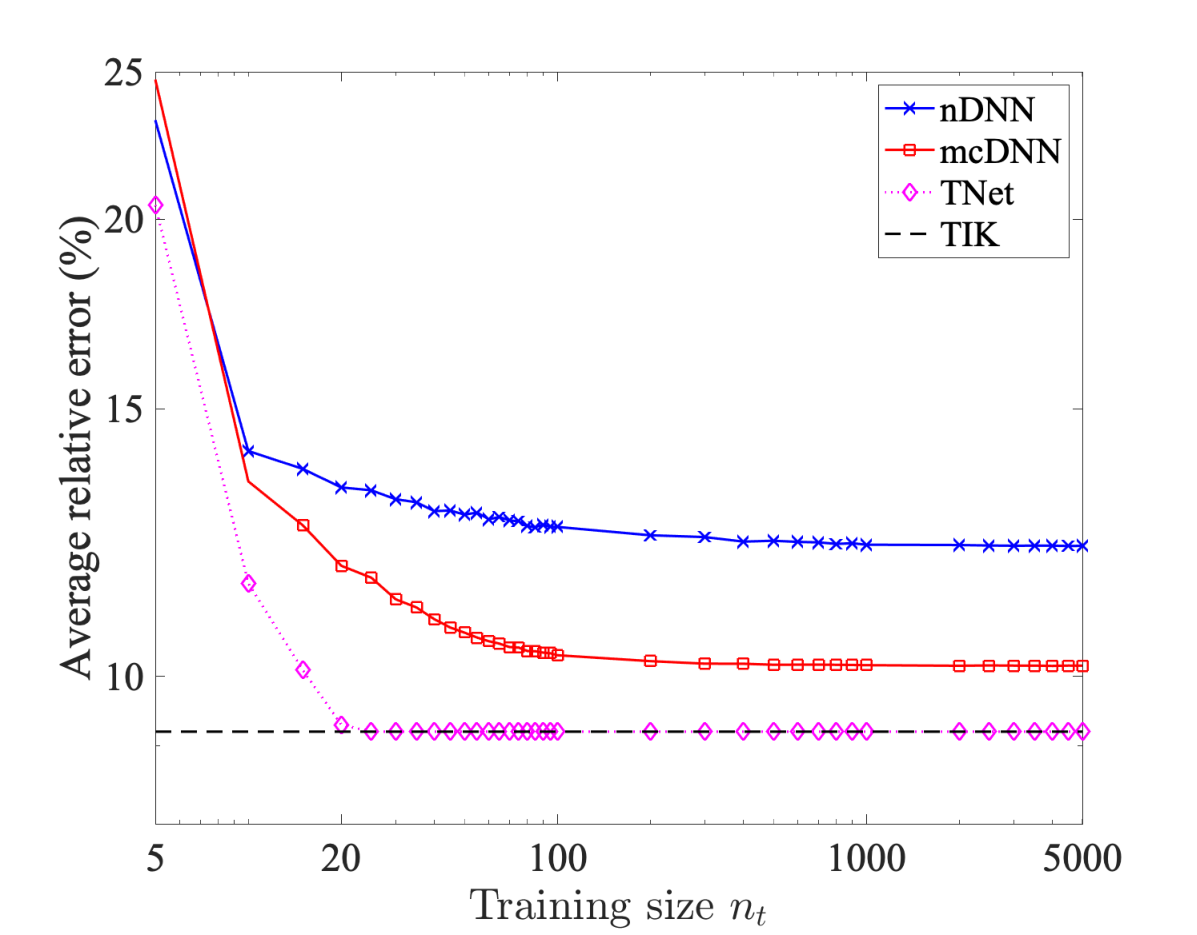
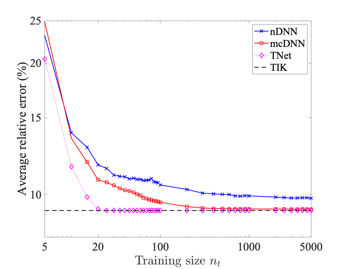
The comparison of relative errors of nDNN, mcDNN, TNet, for Cases I, II, and III with , and the Tikhonov solution is shown in fig. 10. The top row shows the average relative error (see eq. 14) versus the regularization parameter and the training size for all Cases. The pink, red, blue, and black curves are the minimum errors for different training sizes for nDNN, mcDNN, TNet, and for Tikhonov. These curves are re-plotted on the bottom row for clarity. As can be seen, in all cases, TNet solutions match the corresponding Tikhonov solutions when the number of training data size is larger than the number of observation points, regardless of which Case we consider. This numerically verifies the theoretical result in corollary 3, as has full row rank for these scenarios. This appealing property is not observed for nDNN or mcDNN. What we can see is that nDNN and mcDNN approaches provide more accurate reconstructions as we go from Case I to Case III since more distinct data are used to generate the training data set. In particular, mcDNN’s errors are , , and for Cases I, II, and III, respectively. While the optimal regularization parameter for both TNet and mcDNN are closed (in fact exactly for the former with ) to the one for Tikhonov method, for nDNN it erratically varies with the training size . We also observe that, unlike TNet, even though mcDNN solutions are closed to—but not the same as—the Tikhonov ones. This is due to the data-driven nature of as discussed in section 4 after corollary 3. In summary, using Tikhonov solution as the reference, TNet outperforms both mcDNN and nDNN. Solutions of mcDNN and nDNN improve as the number of training data increases though the former is always more accurate: thanks to the model-constrained term (the second term in eq. mcDNN).
| Case I | Case II | Case III |
 |
 |
 |
 |
 |
 |
To understand how much data is needed for each method (except Tikhonov) until the minimum relative error starts saturating, we plot the average relative error at the optimal regularization parameter as a function of the training size for nDNN, mcDNN, TNet, and Tikhonov methods in fig. 11. Again, TNet solutions reach the Tikhonov solutions when the number of training data samples is larger than the number of observation points, regardless of which Case we consider. However, nDNN and mcDNN approaches are still far away from Tikhonov solution even with , though the latter is much more accurate. To be more specific, the relative error obtained by these methods for Case II (left subfigure) with training size between 1000 and 5000 samples have insignificant improvement. This is not surprising as the accuracy of nDNN and mcDNN strongly depends on the information given in the training data set. The interesting point here is that data randomization, as predicted in section 4, improves the generalization (and thus accuracy) of nDNN and mcDNN approaches. Case III (the right subfigure) shows that more distinct training data provides more accurate reconstructions for both nDNN and mcDNN. Furthermore, it is noticeable that mcDNN, owing to the model-constrained term, converges to TIK at far fewer train data samples compared to nDNN. In particular, around 500 training samples mcDNN quality is almost the same as that of Tikhonov solution, while such a highly accurate result for nDNN would need far beyond training samples.
| Case II | Case III |
 |
 |
10.2 2D Burger’s equations
We consider the following viscous 2D Burger’s equations
subject to periodic boundary conditions, initial velocity components , , and viscosity coefficient . The spatial domain is discretized with and mesh points in and directions, respectively, while the temporal domain is subdivided into time steps (including the initial time step ). In this problem, the goal is to invert for the initial -velocity from 20 pointwise values of the vorticity (see the definition below) at the final time .
Construction of train and test data sets. To generate training data for learning the inverse map, we draw periodic samples of using a truncated Karhunen-Loève expansion
where , and are eigenpairs of the covariance with periodic boundary conditions. Next, we discretize an initial vorticity , denoted as , and we solve the Burgers’ equations via a finite difference method to compute the discrete x-velocity component at the final time: . Finally, the values of at 20 locations are extracted and corrupted with an additive white noise to form . An example of a pair of is shown in the middle column of fig. 15.
Similar to the heat conductivity inverse problem in section 5.1, we consider two cases of train data. Case I: Fully distinct training samples are used; and Case II: we first pick a number of distinct baseline samples smaller than , and then replicate and randomize them to obtain samples for the training data set. We shall compare and contrast results from nDNN, mcDNN, TNet, and Tikhonov solutions.
Case I: Training with fully distinct data sets . fig. 12 presents the average relative error eq. 14 obtained by different approaches with different regularization values.
As can be observed, for regularization parameter range , regardless of what is, TNet has the highest accuracy, followed by mcDNN and nDNN, respectively. For , mcDNN is most accurate followed by nDNN and TNet. This is not surprising due to two reasons: i) moderately-to-significantly smaller regularization parameter relative to optimal Tikhonov regularization parameter (around ) is under-regularization and hence giving inaccurate results; and ii) TNet aims to learn Tikhonov solutions. Consequently, the accuracy of TNet is best for the regularization parameter inside a neighborhood of the optimal Tikhonov regularization parameter but degrades outside. A more detailed, but similar, discussion of the behavior of TNet as a function of the regularization parameter can be found in section 5.1. Here, we focus on results at the “best” regularization parameters for all methods.
| nDNN | mcDNN | TNet | TIK | |
|---|---|---|---|---|
| 100 | 1.817 | 1.769 | 1.501 | \multirow4*0.805 |
| 200 | 1.573 | 1.516 | 1.294 | |
| 1000 | 1.189 | 1.128 | 1.037 | |
| 2000 | 1.086 | 1.015 | 0.959 |
It is interesting to see that TNet could get more accurate results even with smaller training data sets. For example, trained with TNet has slightly better accuracy (1.501%) compared to mcDNN (1.516%) and nDNN (1.573%) trained with . Unlike the deconvolution and heat conduction examples, TNet behavior as a function of the regularization parameter does not follow Tikhonov closely, even with . This is expected as Burger’s equation is nonlinear and time-dependent, and we have only observations at the final time.
Nevertheless, TNet is still significantly more accurate than mcDNN and nDNN. table 7 provides the summary of relative error eq. 14 obtained by different approaches at the corresponding optimal regularization parameters. Clearly, TNet is more accurate than nDNN and mcDNN approaches (see also fig. 13). Similar to the other examples, unlike nDNN for which the optimal regularization parameter depends on the training data set, TNet and mcDNN have the same optimal regularization parameter as Tikhonov approach regardless of training data. Shown in fig. 13 is the behavior of average error eq. 14 at the optimal regularization parameter as a function of training data size . As can be seen, though mcDNN, TNet and nDNN seem to converge to the Tikhonov solution, TNet has a faster convergence rate.
Case II: Training with . Shown in table 8 are the average relative error eq. 14 for various training data sets. Recall that we start with to generate training data sets with by replication and randomization. As can be observed, using train data sets with more distinct baseline pairs (i.e. with ), and hence richer information, gives a more accurate inverse map for all approaches. Note that, within the same baseline case, nDNN either does not improve or improves slightly when enriching the data with replication and randomization. In contrast, both mcDNN and TNet show better performance, and the latter is more accurate.
\multirow2*
|
\multirow2*TIK | ||||||||
|---|---|---|---|---|---|---|---|---|---|
| nDNN | mcDNN | TNet | nDNN | mcDNN | TNet | ||||
| 100 | 2.732 | 2.596 | 2.077 | 1.817 | 1.805 | 1.566 | \multirow5*0.805 | ||
| 200 | 2.704 | 2.260 | 1.871 | 1.769 | 1.650 | 1.439 | |||
| 500 | 2.725 | 1.958 | 1.669 | 1.764 | 1.692 | 1.360 | |||
| 1000 | 2.705 | 1.789 | 1.576 | 1.755 | 1.515 | 1.276 | |||
| 2000 | 2.707 | 1.715 | 1.489 | 1.761 | 1.373 | 1.150 | |||
The distribution of average relative pointwise errors eq. 13 for nDNN, mcDNN, TNet, and Tikhonov (TIK) over 500 test samples obtained with and are shown in fig. 14. The numbers in the parentheses in the titles of subfigures are the average error eq. 14 incurred by each method. It can be seen that the pointwise error in the TNet reconstruction is closest to that of Tikhonov solution, and nDNN has the largest error. We would like to emphasize that the average error metrics eq. 13 and eq. 14 (or similar) should be used to assess the performance of a neural network prediction as it reflects the overall average behavior of a neural network solution. The reason is that a network prediction can be less accurate for one case but more for another. In practice, after training and testing, we need to predict the inverse solution for a particular data. To see the solution of each method for a particular test sample, we pick a sample from 500 test samples and plot in fig. 15 the corresponding reconstructions from nDNN, mcDNN, TNet and Tikhonov (TIK) methods. Clearly, overall TNet result is in good agreement with TIK, and thus the ground truth, while mcDNN and nDNN results are less accurate. Again, this conclusion does not always hold as there are test samples on which TNet could less accurate than either nDNN or mcDNN.
| nDNN (1.761) | mcDNN (1.373) | TNet (1.150) | TIK (0.805) |
| nDNN | Exact | mcDNN |
| TNet | Final velocity | TIK |