Gamma rays from Fast Black-Hole Winds
Abstract
Massive black holes at the centers of galaxies can launch powerful wide-angle winds that, if sustained over time, can unbind the gas from the stellar bulges of galaxies. These winds may be responsible for the observed scaling relation between the masses of the central black holes and the velocity dispersion of stars in galactic bulges. Propagating through the galaxy, the wind should interact with the interstellar medium creating a strong shock, similar to those observed in supernovae explosions, which is able to accelerate charged particles to high energies. In this work we use data from the Fermi Large Area Telescope to search for the -ray emission from galaxies with an ultra-fast outflow (UFO): a fast (c), highly ionized outflow, detected in absorption at hard X-rays in several nearby active galactic nuclei (AGN). Adopting a sensitive stacking analysis we are able to detect the average -ray emission from these galaxies and exclude that it is due to processes other than the UFOs. Moreover, our analysis shows that the -ray luminosity scales with the AGN bolometric luminosity and that these outflows transfer 0.04 % of their mechanical power to rays. Interpreting the observed -ray emission as produced by cosmic rays (CRs) accelerated at the shock front, we find that the -ray emission may attest to the onset of the wind-host interaction and that these outflows can energize charged particles up to the transition region between galactic and extragalactic CRs.
I Introduction
Accreting super-massive black holes (SMBHs) at the centers of galaxies, often called active galactic nuclei (AGN), have been observed to launch and power outflows, which can have a dramatic impact on the host galaxies themselves, the intergalactic medium, and the intracluster medium (Silk & Rees 1998; McNamara & Nulsen 2007; Somerville et al. 2008; McCarthy et al. 2010; Hopkins & Elvis 2010). One spectacular, well observed, type of outflow are relativistic jets, where particles are accelerated to near the speed of light in narrow collimated beams (often with an opening angle of ), which can extend up to Mpc scales. These relativistic jets shine at all wavelengths, but are easily studied in radio, X-rays, and rays when the jet axis is not far from our line of sight. Black-hole winds (King & Pounds 2015), on the other hand, are AGN outflows that are not collimated and are generally more difficult to detect, although no less important. Indeed, AGN winds have been proposed as the mechanism able to regulate the co-evolution of the galaxy and its central SMBH, which is observed in the scaling of the black-hole mass and the bulge velocity dispersion (Gebhardt et al. 2000; Ferrarese & Ford 2005; Kormendy & Ho 2013). AGN winds that are powerful enough can heat up and eject the gas from the galaxy, regulating the growth of both the galaxy itself and the black hole.
The most powerful AGN winds can reach velocities of 0.10.3c (Chartas et al. 2002; Pounds et al. 2003; Reeves et al. 2003; Tombesi et al. 2010b) and can carry enough energy to unbind the gas of the stellar bulge (King & Pounds 2015). Some of these winds have been identified in nearby AGN through X-ray observations of blue-shifted Fe K-shell absorption lines (Reeves et al. 2003; Tombesi et al. 2010b; Tombesi et al. 2010a; Tombesi et al. 2012; Gofford et al. 2013).
These winds, which have been dubbed ultra-fast outflows (UFOs), are made of highly ionized gas and are likely launched from near the SMBH (King & Pounds 2003). Their wide solid angle [, (Gofford et al. 2015)] and fast velocity allow UFOs to transfer a significant amount of kinetic energy from the AGN to the host galaxy. They are also believed to be common in nearby AGN (King & Pounds 2015).
UFOs, while traveling outward, interact and shock the interstellar medium (King 2010, ISM,), producing a reverse shock and a forward shock. The reverse shock decelerates the wind itself while the forward shock travels through the galaxy with a velocity in the 200-1000 km s-1 range and leads to the formation of a bubble of hot, tenuous gas, e.g., Zubovas & King 2012. Because of the cooling, the phase and velocity of the outflow should change, eventually leading to the formation of low-velocity molecular outflows, commonly observed in many ultra-luminous infrared galaxies (Cicone et al. 2014; Feruglio et al. 2015, see e.g.). Indeed, there are a handful of objects like IRAS 17020+4544 (Longinotti et al. 2018) and Mrk 231 (Feruglio et al. 2015) where both a UFO and molecular outflow have been detected and found in agreement with the prediction of the energy-conserving outflow model, which is the basis of AGN feedback (Fabian 2012).
UFOs have velocities comparable to (or even larger than) those of the ejecta launched in supernova explosions, which are known to shock the ISM and accelerate cosmic rays (CRs). Gamma-ray emission is a signature of the interaction of relativistic charged particles with ambient gas and photon fields and has been observed in many cases in supernova remnants (Acero et al. 2016). Given the similarity, in this work we search for the -ray emission from UFOs using the Large Area Telescope (Atwood et al. 2009, LAT)] on board the Fermi Gamma-ray Space Telescope (Atwood et al. 2009).
Models of the -ray emission from AGN outflows (Wang & Loeb 2016a; Lamastra et al. 2017) show them to be weak emitters, with -ray luminosities of , which explains why UFOs have not yet been detected by the LAT11 1 No -ray source from the 4FGL catalog (Abdollahi et al. 2020) is a associated to a UFO.. Here, we adopt a different strategy and search for the collective -ray emission from a sample of UFOs using a stacking technique.
The paper is organized as follows. In II and III we describe the sample selection and the data analysis. Results are presented in IV, with additional tests discussed in V. VI reports the theoretical interpretation for the observed -ray emission, while a discussion is reported in VII. Finally, VIII reports our conclusions.
II Sample Selection
We start from a sample of 35 sources that have been identified as UFOs through X-ray observations (Reeves et al. 2003; Tombesi et al. 2010b; Tombesi et al. 2010a; Tombesi et al. 2012; Gofford et al. 2013). We have verified that none of the objects are positionally coincident with any known -ray sources reported in the 4FGL (Abdollahi et al. 2020). From the initial sample we make the following cuts. First, we only keep the radio-quiet sources (as specified in the original references) to avoid contamination of the signal from the relativistic jet. Furthermore, we only select sources that are nearby () with a mildly relativistic wind velocity (). The former cut is motivated by the expected low luminosity of the UFO emission (Wang & Loeb 2016a), and the latter cut is motivated by the fact that the -ray emission is predicted to scale with the kinetic power of the outflow (Wang & Loeb 2016a; Lamastra et al. 2017). After making these cuts we are left with 11 sources, which we use as our benchmark sample. The details of these sources are reported in Table 1.
Table 2 reports additional properties of our sample of UFOs, including the bulge velocity dispersion, 1.4 GHz radio flux and total (8-1000 m) IR luminosity. Figure 1 shows that the UFOs considered here obey the M- relation well (Gültekin et al. 2009; Woo et al. 2010), strengthening the evidence that these outflows operated in the energy-conserving phase in the past (King & Pounds 2015). Finally, the origin of the radio emission in radio-quiet AGN is not very clear and it is likely due to a number of phenomena including AGN winds, star formation, free-free emission from photo-ionized gas and AGN coronal activity (Panessa et al. 2019). For these reasons, the radio fluxes reported in Table 2 are interpreted as upper limits to the synchrotron emission from accelerated electrons, as discussed in Section VI.
We note that there are alternative models explaining the absorption features as produced not by an outflowing wind, but as resonant absorption by highly ionized iron in the accretion disk (Gallo & Fabian 2011). However, this model has difficulties explaining several of the observed properties of the UFO features like the presence of P-Cygni profiles (Nardini et al. 2015; Chartas et al. 2016), or the correlation between outflow velocity and the AGN bolometric luminosity (Saez & Chartas 2011; Matzeu et al. 2017).
| Name | RA | DEC | Type | Redshift | Velocity | log | log | log | log | 95% UL () |
|---|---|---|---|---|---|---|---|---|---|---|
| Ark 120 | 79.05 | 0.15 | Sy1 | 0.033 | 0.27 | 8.2 0.1 | 46.2 1.3 | 45.0 | 7.5 | |
| 44.2 | ||||||||||
| 44.6 | ||||||||||
| MCG-5-23-16 | 146.92 | 30.95 | Sy2 | 0.0084 | 0.12 | 7.6 1.0 | 42.7 1.0 | 44.3 0.2 | 44.1 | 4.3 |
| NGC 4151 | 182.64 | 39.41 | Sy1 | 0.0033 | 0.105 | 7.1 0.2 | 41.9 | 43.1 0.5 | 44.1 | 10.6 |
| 42.9 | ||||||||||
| 43.9 | ||||||||||
| 42.9 | ||||||||||
| 43.2 | ||||||||||
| 43.4 | ||||||||||
| PG 1211+143 | 183.57 | 14.05 | Sy1 | 0.081 | 0.13 | 8.2 0.2 | 43.7 0.2 | 46.9 0.1 | 45.7 | 3.7 |
| 44.8 | ||||||||||
| 44.7 | ||||||||||
| 45.0 | ||||||||||
| 45.1 | ||||||||||
| NGC 4507 | 188.90 | 39.91 | Sy2 | 0.012 | 0.18 | 6.4 0.5 | 44.6 1.1 | 44.3 | 3.4 | |
| NGC 5506 | 213.31 | 3.21 | Sy1.9 | 0.006 | 0.25 | 7.3 0.7 | 43.3 0.1 | 44.7 0.5 | 44.3 | 6.4 |
| Mrk 290 | 233.97 | 57.90 | Sy1 | 0.030 | 0.14 | 7.7 0.5 | 43.4 0.9 | 45.3 1.2 | 44.4 | 4.5 |
| Mrk 509 | 311.04 | 10.72 | Sy1 | 0.034 | 0.17 | 8.1 0.1 | 43.2 | 45.2 1.0 | 45.2 | 9.5 |
| 44.3 | ||||||||||
| 45.3 | ||||||||||
| 44.3 | ||||||||||
| 44.5 | ||||||||||
| 44.7 | ||||||||||
| SWIFT J2127.4+5654 | 321.94 | 56.94 | Sy1 | 0.014 | 0.23 | 7.2 | 42.8 0.1 | 45.6 0.5 | 44.5 | 9.1 |
| MR 2251-178 | 343.52 | 17.58 | Sy1 | 0.064 | 0.14 | 8.7 0.1 | 43.3 0.1 | 46.7 0.7 | 45.8 | 7.4 |
| NGC 7582 | 349.60 | 42.37 | Sy2 | 0.0052 | 0.26 | 7.1 1.0 | 43.4 1.1 | 44.9 0.4 | 43.3 | 4.7 |
Note. — Our sample is comprised of 11 sources with and . The first superscript on the source name indicates the reference for the detection, and the second superscript indicates the reference for the UFO parameters (columns ), where and are the minimum and maximum kinetic powers. Values for the bolometric luminosity are taken from the literature, with the reference indicated by the superscript. For sources with numerous determinations we also give the mean value in boldface text. The -ray flux ( GeV) upper limit (UL) is calculated at the 95% confidence level, using a photon index of –2.0. Tombesi et al. 2010a; Gofford et al. 2013; Tombesi et al. 2012; Gofford et al. 2015; Vasudevan et al. 2010; Vasudevan & Fabian 2007; Vasudevan & Fabian 2009; Peterson et al. 2004; Crenshaw & Kraemer 2012; Kaspi et al. 2005; Kaspi et al. 2005; Alonso-Herrero et al. 2011.
| Name | Velocity Dispersion | 1.4 GHz Radio Flux | IR Lum. |
|---|---|---|---|
| [mJy] | log (L⊙) | ||
| Ark 120 | 184, 238 | 12.4 | 11.0 |
| MCG-5-23-16 | 152, 192 | 14.3 | 9.6 |
| NGC 4151 | 94, 119 | 347.6 | 10.2 |
| PG 1211+143 | 4.3 | ||
| NGC 4507 | 146, 156 | 67.4 | 10.5 |
| NGC 5506 | 160, 200 | 355 | 10.5 |
| Mrk 290 | 109, 111 | 5.32 | 10.3 |
| Mrk 509 | 172, 196 | 19.2 | 10.5 |
| SWIFT J2127.4+5654 | 6.4 | 10.4 | |
| MR 2251-178 | 16 | ||
| NGC 7582 | 110, 116 | 270 | 10.6 |
Note. — The second column gives velocity dispersion measurements taken from the literature, with the references indicated by the superscripts. Measurements were found for 8/11 sources, and we provide minimum and maximum values (separated by a comma). For sources with just one reference, the range is due to statistical error only, and for sources with two references, the range also includes the systematic error due to the different estimates. Note that most published estimates of the black-hole mass for NGC 4507 are based on velocity dispersion and [O III] line widths, and thus they are not independent measures. In quantifying the uncertainty in Figure 1 we also use black-hole mass values from Bian & Gu 2007; Beifiori et al. 2012; Nicastro et al. 2003. Woo et al. 2010; Grier et al. 2013; Onken et al. 2014; Marinucci et al. 2012; Bennert et al. 2015; Hyperleda; NVSS (Condon et al. 1998); IRAS (Kleinmann et al. 1986; Moshir & et al. 1990).
III Data Analysis
III.1 Data
We analyze data collected by Fermi-LAT between 2008 August 04 to 2019 September 10 (11.1 years). The events have energies in the range 1800 GeV and are binned in 8 bins per decade. The pixel size is . To reduce contamination from the Earth’s limb we use a maximum zenith angle of . We define a region of interest (ROI) centered at the position of each UFO source. We use the standard data filters: DATA_QUAL0 and LAT_CONFIG==1. The analysis is performed using Fermipy (v0.18.0)22 2 Available at https://fermipy.readthedocs.io/en/latest/, which utilizes the underlying Fermitools (v1.2.23).
We select photons corresponding to the P8R3_SOURCE_V2 class (Atwood et al. 2013). In order to optimize the sensitivity of our stacking technique we implement a joint likelihood analysis with the four point spread function (PSF) event types available in the Pass 8 data set33 3 For more information on the different PSF types see https://fermi.gsfc.nasa.gov/ssc/data/analysis/documentation/Cicerone/Cicerone_Data/LAT_DP.html.. The data is divided into quartiles corresponding to the quality of the reconstructed direction, from the lowest quality quartile (PSF0) to the best quality quartile (PSF3). Each sub-selection has its own binned likelihood instance that is combined in a global likelihood function for the ROI. This is easily implemented in Fermipy by specifying the components section in the configuration file. Each PSF type also has its own corresponding isotropic spectrum, namely, iso_P8R3_SOURCE_V2_PSFi_v1, for ranging from 03. The Galactic diffuse emission is modeled using the standard component (gll_iem_v07), and the point source emission is modeled using the 4FGL catalog (gll_psc_v20). In order to account for photon leakage from sources outside of the ROI due to the PSF of the detector, the model includes all 4FGL sources within a region. The energy dispersion correction (edisp_bins=–1) is enabled for all sources except the isotropic component.
III.2 Analysis
In the local Universe () UFOs are predicted to have a -ray luminosity of (Wang & Loeb 2016a), making them too faint to be detected individually by Fermi-LAT. Indeed, adopting the average photon index in the 4FGL of we derive a GeV flux of ph cm-2 s-1, for a source with a luminosity of 1040 erg s-1 at (the median redshift of our sample). This flux is 2.5 times fainter than the weakest source reported in the 4FGL. We therefore analyze our source sample using a stacking technique. This technique has been developed previously and has been successfully employed for multiple studies, i.e. upper limits on dark matter interactions (Ackermann et al. 2011), detection of the extragalactic background light (Abdollahi et al. 2018), extreme blazars (Paliya et al. 2019), and star-forming galaxies (Ajello et al. 2020b).
The main assumption that we make for the stacking technique is that the sample of UFOs we are considering can be characterized by average quantities like the average flux and the average photon index (when we model their spectra with a power law). There are then two steps to the method. In the first step the model components are optimized for each ROI using a maximum likelihood fit. We evaluate the significance of each source in the ROI using the TS, which is defined as:
| (1) |
where is the likelihood for the null hypothesis, and L is the likelihood for the alternative hypothesis44 4 For a more complete explanation of the TS resulting from a likelihood fit see Mattox et al. 1996 and https://fermi.gsfc.nasa.gov/ssc/data/analysis/documentation/Cicerone/Cicerone_Likelihood/.. For the first iteration of the fit, the spectral parameters of the Galactic diffuse component (index and normalization) and the isotropic component are freed. In addition, we free the normalizations of all 4FGL sources with TS25 that are within of the ROI center, as well as sources with TS500 and within . Lastly, the UFO source is fit with a power-law spectral model, and the spectral parameters (normalization and index) are also freed. In the first step we also find new point sources using the Fermipy function find_sources, which generates TS maps and identifies new sources based on peaks in the TS. The TS maps are generated using a power-law spectral model with an index of . The minimum separation between two point sources is set to , and the minimum TS for including a source in the model is set to 16.
In the second step 2D TS profiles are generated for the spectral parameters of each UFO source, where the TS is defined as in Eq. 1. We scan photon indices from –1 to –3.3 with a spacing of 0.1 and total integrated photon flux (between 1–800 GeV) from to with 40 logarithmically spaced bins, freeing just the parameters of the diffuse components. For this step the power-law spectra of the UFOs are defined in terms of the total flux (), integrated between the minimum energy () and the maximum energy ():
| (2) |
Note that the likelihood value for the null hypothesis is calculated at the end of the first step by removing the UFO source from the model. Since we perform a joint likelihood in the different PSF event types (PSF0 PSF3), the total profile for each source is obtained by adding the profiles from each of the four event types. Lastly, the TS profiles for all sources are added to obtain the stacked profile. The TS is an additive quantity, and so the stacked profile gives the statistical significance for the combined signal.
We validated the stacking method relying on a set of Monte Carlo simulations that reproduce the Fermi-LAT observations. In these tests, the simulations include the isotropic and Galactic emission, as well as an isotropic population of point sources resembling blazars, which account for the vast majority of sources detected by Fermi-LAT. Faint, below-threshold “blazars” are included in the synthetic sky following the models of Ajello et al. 2015. Using this setup two different tests were performed. The stacking analysis was performed at 60 random “empty” positions, i.e., positions away from bright detected sources. This analysis yielded no detection, confirming that the technique does not generate spurious detections. The second set of tests was aimed at characterizing the detected signal. The stacking was performed for 60 simulated sources whose flux was extracted from a power-law distribution with index and minimum and median flux of respectively and . The photon indices were extracted from a Gaussian distribution with average 2.21 and dispersion of 0.2. The values derived from the stacking analysis (flux = and index of ) are in agreement with the inputs, showing that our analysis successfully retrieves the average quantities of a population of sources. Moreover, the likelihood profile would not show a significant peak if those average quantities were not representative of the population.
IV Results
IV.1 Stacked TS Profile for The Benchmark Sample
The log-likelihoods (i.e. logL) are maximized with the optimizer MINUIT (James & Roos 1975), and we have verified that each fit converges properly, as indicated by the MINUIT outputs of and . The 95% flux upper limits from the preprocessing step are reported in Table 1.
The stacked profile for our UFO sample is shown in Figure 2. The maximum TS is 30.1 (5.1)55 5 The conversion from TS to has been performed on the assumption that the TS behaves asymptotically as a distribution with 2 d.o.f (Mattox et al. 1996). Additionally, the Akaike information criterion test also shows the null hypothesis to be highly disfavored with a relative likelihood of . , corresponding to a best-fit index of and a best-fit photon flux (1800 GeV) of . The 68%, 90%, and 99% significance contours are overlaid on the map, and as can be seen the spectral parameters are well constrained. The source with the overall highest individual TS is NGC 4151, having a maximum value of 21.2 (4.2 ), corresponding to a best-fit index of and a best-fit flux of . The stacking analysis excluding NGC 4151 yields a maximum TS of 15.1 (), corresponding to a best-fit index of and a best-fit flux of .

IV.2 Spectral Energy Distribution of UFOs
The best-fit SED for our UFO sample is shown in Figure 3. The butterfly plot is constructed by sampling the range of parameter values that are within the 68 % confidence contour of the stacked profile. In addition, we calculate the SED flux in 3 logarithmically spaced bins between 1800 GeV. In every bin, we fix the power law index of the UFOs to and leave all other parameters free to vary. As can be seen, these data points are in agreement with the best-fit SED model. To characterize the UFO spectrum at low energy we repeat the stacking analysis in the energy range 0.1 1 GeV, which yields a 95% flux upper limit () of . We also overlay our best-fit hadronic model presented in VI.



IV.3 Bins of Bolometric Luminosity and Kinetic Power
We test whether the -ray emission from UFOs scales with AGN bolometric luminosity and outflow kinetic power. To properly take the distance of each source into account, we stack in the luminosity-index space. We take estimates of the bolometric luminosity from the literature, as reported in Table 1. Such estimates can be obtained by applying a correction factor to a certain flux, typically the 5100 Å optical emission, the 1450 Å UV emission, or the 210 keV X-ray emission. Alternatively, the bolometric luminosity can be determined by fitting an SED to the broad-band emission. In any case, the absorption from the host galaxy must be corrected for, which has a large dependence on the viewing angle of the source, and can introduce a rather significant uncertainty. In addition, the contribution from the host galaxy emission also needs to be corrected for (i.e., UV/IR/Opt emission from the galactic disk). Most of the AGN emission is observed in the optical/UV, while 10% is emitted in the X-ray, and thus a broadband SED fitting ensures a more accurate determination of the bolometric luminosity. We therefore search the literature for the most reliable estimates of the bolometric luminosity, and rely on the X-ray determination for only 2 sources (MCG-5-23-16 and SWIFT J2127.4+5654) for which no other estimates could be found. For sources with multiple estimates we take the geometric mean. The mean of the bolometric luminosity of our sample is , and we create two bins around this value.
The stacked profiles for the two bins are shown in Figure 4. The first bin has 5 sources, with a mean redshift of 0.007. The maximum TS is 28.5 (5.0 ), corresponding to a best-fit index of and a best-fit luminosity of . The second bin has 6 sources, with a mean redshift of 0.04. The maximum TS is 9.9 (2.7 ), corresponding to a best-fit index of and a best-fit luminosity of . The total TS (bin 1 + bin 2) for the stacking in bins is 38.4, compared to 30.1 for the full stack.
We also stack the -ray luminosity in bins of kinetic power. In general the kinetic power as determined from X-ray observations has a large uncertainty, as can be seen in Table 1. Minimum and maximum values are typically reported, corresponding to minimum and maximum radii of the outflow. We use the geometric mean of the minimum and maximum estimates for our calculations (also incorporating statistical uncertainties in the range). We create two bins around the mean kinetic power, which has a value of . The stacked profiles for the two bins turn out to be the same as for the bolometric bins, as shown in Figure 4.
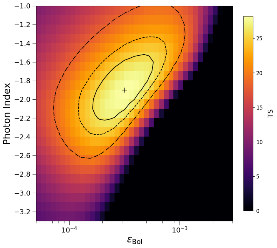
To further verify the relations found above for the stacking in bins, we perform the stacking analysis using both bolometric efficiency () and kinetic power efficiency (). This is done by evaluating for each source the TS of a given (or ) and using that efficiency value, the bolometric luminosity (or kinetic power), and the distance of the source to transform to -ray flux (for a given photon index). Results for these fits are shown in Figure 5. The left panel shows the bolometric efficiency, with a best-fit value of , corresponding to a best-fit index of , and a maximum TS of 28.2 (5 ). The right panel of Figure 5 shows the kinetic power efficiency, with a best-fit value of , corresponding to a best-fit index of , and a maximum TS of 23.0 (4.4 ). We note that the best-fit index from the efficiency analysis is slightly harder than the one found by the flux-index stacking, but compatible within 1 uncertainties. The small shift observed in the best-fit index value is due to how the TS profiles are weighted differently when stacking in efficiency with respect to flux.
The result for stacking in bolometric luminosity and kinetic power are summarized in Figure 6. The left panel shows the -ray luminosity versus bolometric luminosity, and the right panel shows the -ray luminosity versus UFO kinetic power. The black data points are for stacking in bins, and the corresponding best-fit efficiency, along with the 1 confidence interval, is plotted with the green band. Also plotted are lines for different efficiencies under the assumption of a linear scaling. As can be seen, the results on the efficiencies are in very good agreement with the stacking in bins.
In the left panel of Figure 6 we also overlay the predicted scaling of with from Liu et al. 201866 6 Our derivation is made converting the peak 1 GeV luminosities (reported in their Figure 5) to the 1-800 GeV energy range using the best-fit spectral index of .. As can be seen, Liu et al. 2018 predict a nearly linear scaling between the logarithms of the two luminosities (over their range) with an efficiency of , which is in reasonably good agreement with the one measured here.
IV.4 Representative Luminosity of the Sample
Because the 11 UFO galaxies are detected at fairly different distances, we adopt a weighting scheme to compute the representative luminosity of the sample. In this framework , where and are the luminosity and the TS for the galaxy at the global best-fit position (1-800 GeV flux of 2.5 ph cm-2 s-1 and photon index of 2.1) and . The representative luminosity is found to be erg s-1 and would correspond to an effective redshift of (adopting the above best-fit parameters). This luminosity is in very good agreement with the one obtained scaling the average bolometric luminosity erg s-1 by the best-fit efficiency (). The effective redshift is also very close to the median redshift of the sample ( vs. ) making the TS-weighted luminosity compatible with the median -ray luminosity of the sample.
IV.5 Simulations
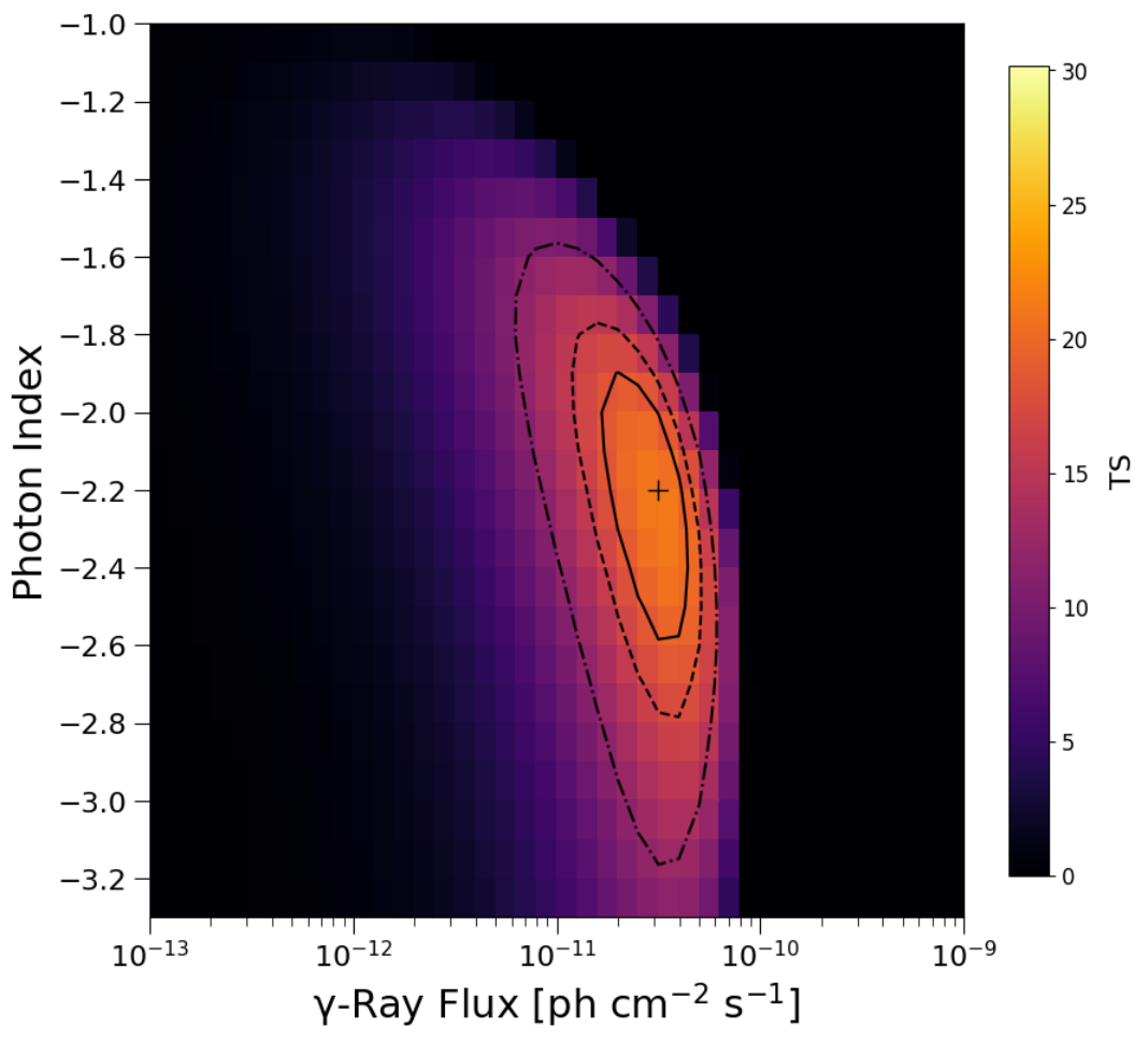
The results presented here are validated using Monte Carlo simulations. We simulate the fields of the 11 UFOs considering the Galactic and isotropic emission (modeled as gll_iem_v07 and iso_P8R3_SOURCE_V2_v1, respectively), background sources from the 4FGL catalog, and our test source at the position of the UFO in each ROI. The UFO spectral parameters are set to be the same as the best-fit values from the data, i.e. index and flux . For simplicity we use the standard event type (evtype), i.e. we do not use the four different PSF event types. The data is simulated using the simulate_roi function from Fermipy. The simulation is created by generating an array of Poisson random numbers, where the expectation values are drawn from the model cube77 7 More information on generating the simulations is available at https://fermipy.readthedocs.io/en/latest/fermipy.html.. Finally, we run our stacking pipeline on the simulated data. We recover the input values, with a best-fit index of , a best-fit flux of , and a maximum TS of 21.2 (). The stacked profile is shown in Figure 7. Overall the results from the simulation are consistent with the real data.
V Additional Tests
V.1 Control Sample
We repeat the analysis with a sample of 20 low redshift () radio-quiet AGN that do not have UFOs. The sources were selected from the samples of Tombesi et al. 2010a and Igo et al. 2020 for which no UFO was found. The sample of Tombesi et al. 2010a is based on absorption features, while the sample of Igo et al. 2020 uses the excess variance method. Of the 20 sources in our control sample, there are 10 sources in common between the two studies, 4 additional sources from Tombesi et al. 2010a, and 6 additional sources from Igo et al. 2020. For reference, the list of sources in the control sample is given in Table 3. Figure 8 shows that the benchmark and control samples are well matched in X-ray luminosity and redshift.
Results for the stacked profile are shown in Figure 9. No signal is detected, with a maximum TS of 1.1. Using the profile likelihood method and a photon index of 2.0, the upper limit on the flux (1800 GeV) at the 95% confidence level is . This supports the interpretation of the -ray emission being due to the outflow rather than other processes in AGN.
| Name | RA | DEC | Redshift | IR Lumin. | 1.4 GHz flux |
|---|---|---|---|---|---|
| log (L⊙) | [mJy] | ||||
| ESO 198-G024 | 39.58 | -52.19 | 0.046 | ||
| Fairall 9 | 20.94 | -58.81 | 0.047 | ||
| H 0557-385 | 89.51 | -38.33 | 0.034 | ||
| MCG+8-11-11 | 88.72 | 46.44 | 0.020 | 11.1 | 286 |
| Mrk 590 | 33.64 | -0.77 | 0.026 | ||
| Mrk 704 | 139.61 | 16.31 | 0.029 | ||
| NGC 526A | 20.98 | -35.07 | 0.019 | 10.5 | 13.9 |
| NGC 5548 | 214.50 | 25.14 | 0.017 | ||
| NGC 7172 | 330.51 | -31.87 | 0.0090 | 10.4 | 37.6 |
| NGC 7469 | 345.82 | 8.874 | 0.016 | 11.6 | 181 |
| ESO 113-G010 | 16.32 | -58.44 | 0.027 | ||
| ESO 362-G18 | 79.90 | -32.66 | 0.012 | ||
| IRAS 17020+4544 | 255.88 | 45.68 | 0.060 | 11.6 | 129 |
| MS22549-3712 | 344.41 | -36.94 | 0.039 | ||
| NGC 1365 | 53.40 | -36.14 | 0.0055 | 10.9 | 534 |
| NGC 4748 | 193.05 | -13.41 | 0.015 | 10.4 | 14.3 |
| Mrk 110 | 141.30 | 52.29 | 0.035 | ||
| IRAS 05078+1626 | 77.69 | 16.50 | 0.018 | 10.8 | 6.3 |
| ESO 511-G30 | 214.84 | -26.64 | 0.022 | ||
| NGC 2110 | 88.05 | -7.46 | 0.0078 | 10.3 | 300 |
Note. — See Tombesi et al. 2010a and Igo et al. 2020 for further details of the sources. The IR luminosity is reported in the 8-1000 m range and derived from IRAS (Kleinmann et al. 1986; Moshir & et al. 1990). The radio fluxes are derived from NVSS (Condon et al. 1998).
.

V.2 Alternative UFO Samples
The fractional excess variance method was recently used in Igo et al. 2020 to search for UFOs in the samples of Tombesi et al. 2010a and Kara et al. 2016. Overall, the results are in agreement with the past literature, finding that UFOs are a relatively widely observed phenomena in nearby AGN. However, there are differences with respect to previous studies in regards to which sources are classified as UFOs, and the corresponding UFO parameters.
As the authors mention in Igo et al. 2020, their method relies on the variability of the strength of the emission (or absorption) features and is less sensitive in detecting cases where these features may vary in energy. The excess variance method is well suited for detecting UFOs in objects that show small changes in the energy of the UFO, but large changes of the equivalent width for the same energy. This is one reason why the excess variance method can potentially miss objects that were detected in spectral-timing analyses that model individual spectra in single epochs.
As an additional a-posteriori test we perform our stacking analysis with the UFO sample determined in Igo et al. 2020, relying on sources classified as either likely outflows or possible outflows therein. Additionally, we use the same selection criterion as for our benchmark sample, i.e. and . This gives a sample of 18 sources. The maximum TS is 13.0 (3.2), corresponding to a best-fit flux of and a best-fit index of . These results, although less significant, are in good agreement with those from our benchmark sample and show that there is -ray emission associated to UFOs independently of how these sources were selected.
V.3 Emission from Star-formation activity
Star-forming galaxies are known ray emitters because of their CR population, which is accelerated at the shock fronts of supernova remnants and pulsar wind nebulae (Ajello et al. 2020a). The ensuing -ray emission is known to correlate well with the total infrared (IR) luminosity (8-1000 m), which is a tracer of star formation.
We find that the average total IR luminosity is (see Table 2). According to the correlation reported in Ajello et al. 2020a this implies an average -ray luminosity (1 GeV) of 2.2 erg s-1. This is about 40 times smaller than the observed luminosity and implies that the contamination due to star-formation activity to the signal observed in the UFO sample is negligible.
As an additional test we searched for IR fluxes for the galaxies in the control sample (see Table 3). We could find data for nine galaxies with an average total IR luminosity of (compared to 10.4 for the benchmark sample). The stacking of this subset of galaxies in the control sample yields no detection (TS=0.04 and 95% flux UL=) confirming that the contamination of the signal due to star formation is negligible.
V.4 Emission from Potential Jets in Radio-quiet AGN
The vast majority of the -ray sources detected by the LAT are powered by relativistic jets closely aligned to the line of sight (Ajello et al. 2020c). Some of the sources in our sample, particularly NGC 4151, may have a jet. However, there are several reasons why the -ray emission that we observe is unlikely to be produced by the jets, which may be present in these radio-quiet AGN. The best-studied system88 8 Other sources like NGC 5506 and NGC 7582 do not have resolved radio jets down to 0.1′′, while MCG-5-23-16 has a resolved morphology suggesting the presence of a jet (Orienti & Prieto 2010). is NGC 4151, for which an elongated series of knots, possibly associated with a jet, have been detected in radio (Johnston et al. 1982; Wilson & Ulvestad 1982). This jet has an angle of with respect to the line of sight and a speed 0.04 (Williams et al. 2017). This is among the lowest speeds measured for a jet and indicates non-relativistic motion, likely due to thermal plasma (Ulvestad et al. 2005). NGC 4151’s jet lies on the opposite end of the spectrum of jets detected by the LAT, which are aligned often within 1 (Pushkarev et al. 2017), highly relativistic (Lister et al. 2016), dominated by non-thermal emission, and found only in radio-loud AGN (Ajello et al. 2020c).
Moreover, the emission from jets is not expected to correlate with the bolometric luminosity of radio-quiet AGN or the outflow kinetic power. It should also be noted that the sources in our sample follow the trend indicating a contribution to the radio luminosity from the hot AGN corona (Smith et al. 2020). Finally, the analysis of winds and jets in a sample of radio-loud AGN provides evidence for a wind-jet bimodality, where winds are the strongest when jets are the weakest (Mehdipour & Costantini 2019, as measured by the radio-loudness parameter).
More importantly, the same 9 galaxies in the control sample for which we could find IR data also have 1.4 GHz fluxes (see Table 3). This sample is well matched in terms of radio fluxes and redshift to our benchmark sample and as reported above yields no -ray detection.
VI SED Modeling
We assume as in Wang & Loeb 2016a and Lamastra et al. 2017, that the -ray emission is dominated by hadronic processes resulting from diffusive shock acceleration (DSA). In order to model these processes in detail, we first calculate proton distributions using the Cosmic Ray Analytical Fast Tool (CRAFT), a code that uses a semi-analytical formalism for DSA described in (Blasi 2002; Amato & Blasi 2006; Caprioli et al. 2010) and references therein. CRAFT self-consistently solves the diffusion-convection equation (e.g., Skilling 1975) for the transport of non-thermal particles in a quasi-parallel, non-relativistic shock, including the dynamical effects of both accelerated particles and the magnetic turbulence they generate Caprioli 2011; Caprioli 2012. CRAFT also uses microphysical information (particle injection, diffusion, magnetic field amplification) tuned on self-consistent kinetic plasma simulations of non-relativistic shocks (Caprioli & Spitkovsky 2014a; Caprioli & Spitkovsky 2014b; Caprioli & Spitkovsky 2014c; Caprioli et al. 2015; Haggerty & Caprioli 2019). Thus, given basic information about UFO shock hydrodynamics (age, velocity, and ambient density), CRAFT self-consistently predicts an instantaneous proton distribution.
To model the cumulative photon distribution of a UFO, we use the hydrodynamic model for the forward shock evolution calculated in Liu et al. 2018 and shown in Figure 10. More specifically, Liu et al. 2018 calculate the forward shock evolution (as in Lamastra et al. 2017; Wang & Loeb 2016a; Wang & Loeb 2016b, and elsewhere in the literature) using the thin-shell approximation, in which a spherically symmetric shell of negligible thickness expands due the pressure of a hot bubble inside it. Liu et al. 2018 adopts a broken power law density profile for the ambient gas, inside the disk radius and outside the disk. However, Liu et al. 2018 also includes a flat core in the inner 100 pc of the galaxy to prevent high central densities that are inconsistent with observations, as well as a constant density beyond the virial radius of the galaxy to account for the presence of the intergalactic medium. This profile reproduces well the stellar velocity dispersion in the bulge of the galaxies in our sample (see Figure 1). Both the forward shock evolution and density profile apply to the case of an AGN with a bolometric luminosity of erg s-1 (consistent with our measurement) and are both shown in Figure 10. Of course, the use of a 1D model has limitations; it cannot account for a more complex ambient medium meaning that inferred values such as the forward shock age and radius are only approximate. However, given that the model in Liu et al. 2018 yields -ray spectra in good agreement with observations, this calculation demonstrates that the -ray emission reported in this work can be explained by a population of UFOs with reasonable parameters.
After using CRAFT to calculate the proton distribution produced at each time step of the shock evolution (see Figure 10), the resulting instantaneous distributions are weighted and shifted in energy to account for adiabatic losses as in Diesing & Caprioli 2019. Energy losses due to proton-proton collisions–which are eventually responsible for the UFO’s -ray emission–are also taken into account by calculating the collision rate for each distribution at each time step, assuming a target proton density given by the adiabatically expanded post-shock density of a given shell. We further assume that a proton loses half its energy in a single collision (i.e., we assume an inelasticity , as in Liu et al. 2018). In other words, the accelerated proton population is treated as a series of adiabatically expanding shells, with the outermost shell located at the forward shock. Each of these shells experience proton-proton collisions–and by extension, produce -rays at every time step. Thus, to calculate a UFO’s -ray spectrum at a given time, we simply take these weighted proton distributions and convert them to photon spectra using the radiative processes code naima (Zabalza 2015). We then add these photon spectra together to produce a cumulative SED. Note that Coulomb losses are neglected in this calculation, as they are subdominant for protons with energies GeV (Mannheim & Schlickeiser 1994).
The result is an estimate of a UFO’s SED at every stage of its evolution, as shown in the left panel of Figure 11. We obtain -ray luminosities consistent with those calculated in Liu et al. 2018 and find that the observed -ray emission can be explained by a forward shock that has traveled a distance between kpc from the SMBH (age of yr). The modeled CR and -ray light curves of the UFO are also shown in the right panel of Figure 11. It is worth noting that the total energy in CRs–and thus the UFO’s -ray luminosity –naturally cuts off after roughly ten million years due to the fact that the ambient density in the reference galaxy decreases substantially with radius, thereby reducing the available energy flux across the shock.
We also estimate instantaneous electron distributions from our instantaneous proton distributions by using the formalism in Zirakashvili & Aharonian 2007 and accounting for the effects of both adiabatic and synchrotron losses in our weighting (Diesing & Caprioli 2019, see). To confirm that the UFO’s synchrotron emission remains below the average radio upper limit from Table 2, the relative normalization of these electron distributions is taken to be a factor of a few larger than that needed to fit observations of Tycho’s supernova remnant (Morlino & Caprioli 2012). Again using naima, we then calculate the leptonic emission of a typical UFO from the weighted electron distributions, adding together the contribution of each shell to produce a cumulative SED at a given time step. As shown in Figure 11, the resulting synchrotron emission always falls below the measured average radio emission of the galaxies and the inverse-Compton and bremsstrahlung emissions are a factor fainter than the emission. Note that the inverse-Compton emission is estimated by assuming that electrons scatter off the cosmic microwave background and starlight approximated by a blackbody with temperature T = 3000 K. This emission remains a factor below the one even with an artificially enhanced stellar radiation field of energy density 100 eV cm-3. We also model the inverse-Compton emission assuming electrons scatter off the AGN photon field described in Sazonov et al. 2004, normalized to the bolometric luminosity of the AGN sample, and find that this emission remains a factor below that produced by -decay (and with a much softer spectrum above 30 GeV).
Proton-proton interactions produce rays with energy (Kelner et al. 2006), and thus the observed -ray SED indicates a firm detection of CR protons with energies reaching at least as high as eV. Within our hadronic emission model we derive that the maximum energy of protons accelerated at the forward shock is 1017 eV. This makes AGN winds a potential source of CRs with energies beyond the ‘knee’ of the CR spectrum (i.e., eV) and also likely contributors to the IceCube neutrino flux (Aartsen et al. 2013).
VII Discussion
This work has provided evidence for the existence of a new population of -ray emitters produced by AGN-driven outflows, which in the interaction with the ISM can create strong shocks able to energize charged particles potentially up to the transition region between Galactic and extragalactic CRs. These charged particles produce the observed rays in the interaction with the ISM. According to our and other available models (Liu et al. 2018), the observed emission can be explained by a forward shock that has traveled 20 pc from the central SMBH. As such, the -ray emission from UFOs may signal the onset of the wind-host interaction. We caution the reader, however, that our model relies on a one dimensional description of a galaxy and that it does not include the complex environment in the immediate vicinity of the SMBH. Nevertheless, our results are found to be in reasonably good agreement with previous predictions (Lamastra et al. 2016; Liu et al. 2018).
Most of the outflow energy is deposited in the bubble of hot gas rather than CRs. More precisely, this energy is a factor of 10 larger than what is transferred to accelerated CRs, which is reported in the right panel of Figure 11. For an AGN with (erg s-1)=44.4 the timescale to transfer 1056 erg of energy to the bubble is about 3 million years. This timescale would grow slightly for less powerful AGN. Sgr A*, the SMBH in the center of the Milky Way, has an estimated mass of 4 million M⊙ (Abuter et al. 2019), and was very likely in an active state up to a few hundred years ago (Sunyaev et al. 1993; Koyama et al. 1996). Adopting a bolometric luminosity of (erg s-1)=42.7 (about 1 % of its Eddington luminosity), we find that the timescale to deposit an energy of 1056 erg to the thermal gas is 10 million years. At that point in time, its -ray luminosity would be (erg s-1)38 and would decline modestly in a few hundred years after the end of the AGN activity (Liu et al. 2018, see also). This is in reasonable agreement with the luminosity of the bubbles discovered by Fermi in our galaxy ( = 37.6 erg s-1 (Su et al. 2010)) and the energetics of the thermal gas contained in the larger bubbles (1056 erg) recently discovered by eROSITA (Predehl et al. 2020). Thus, the Fermi and eROSITA bubbles may be the remnant of past UFO-like activity from the SMBH in the center of our galaxy.
It is important to note that the physical implications that can be inferred from the -ray detection are limited by the incompleteness of the current sample of UFOs, as well as the inherent uncertainty relating to the time variability of the UFOs. Indeed, detection of UFOs is limited to 50 AGN (Tombesi et al. 2010b; Kara et al. 2016; Igo et al. 2020), which is by far not a complete sample. Moreover, UFOs have been found in these AGN to vary with time and energy and this has been interpreted as a series of expanding shells (King & Pounds 2015, see e.g.) rather than a continuous outflow like we have assumed here. Although we consider it unlikely, the variability may also impact the selection of a control sample as those AGN may not show a UFO precisely at the time when they were observed, but have otherwise an active UFO. A solution to these issues will be provided with the more sensitive observations that the X-ray Imaging and Spectroscopy Mission (XRISM Science Team 2020, XRISM,) and the Advanced Telescope for High-Energy Astrophysics (Athena99 9 https://www.the-athena-x-ray-observatory.eu) will provide.
VIII Summary and Conclusion
To search for the collective UFO emission, a stacking technique which has been used with success in the past (Abdollahi et al. 2018; Paliya et al. 2019; Ajello et al. 2020b) is adopted. Our sample consists of all radio-quiet UFOs with and , which gives 11 sources in total. We model the UFO (-ray) spectrum with a power law, and we assume that the population can be characterized by an average flux and photon index. A fit to all the regions then optimizes these parameters. We find a TS of 30.1, which corresponds to a detection significance for the UFO emission of 5.1 (2 d.o.f.). The best-fit parameters are measured to be and flux (1-800 GeV) = .
We performed several tests to confirm that the -ray emission is truly related to the presence of UFOs in this sample of galaxies. We employed a control sample of AGN with similar properties to those of the 11 galaxies used above, but lacking UFOs. This sample yields no detectable -ray emission with a (1-800 GeV) flux upper limit of 8.8 ph cm-2 s-1. We also use a sample of UFOs selected in a different way (Igo et al. 2020) than our benchmark sample. These galaxies show a -ray signal whose parameters are in good agreement with those reported above. Moreover, adopting a control sample matched in X-ray flux, IR luminosity, radio flux and redshifts we can exclude that the observed -ray emission arises from star-formation activity or the presence of a weak jet. These tests allow us to conclude that the observed emission is associated to the presence of UFOs in these galaxies.
Observations of AGN winds have shown that AGN transfer a small fraction (15 %) of their bolometric luminosity to the winds. As our analysis indicates, a portion of this transferred luminosity in turn accelerates CRs and produces rays. We find that AGN convert of their bolometric luminosity into rays. We also find that of the wind mechanical power is transferred to rays. For comparison, in the Milky Way galaxy, supernova explosions transfer of their mechanical energy to rays. This shows that AGN winds, if sustained for a few million years, can energize a large fraction of the CR population within a galaxy.
The physical model for the UFO SED is calculated by assuming that the -ray emission is dominated by hadronic processes resulting from diffusive shock acceleration. For typical UFO shock velocities and densities, a leptonic origin of the -ray emission is disfavored, in that inverse-Compton scattering and bremsstrahlung of relativistic electrons would produce steeper -ray spectra with a lower normalization. The observed -ray SED indicates a firm detection of CR protons with energies reaching at least as high as eV.
Within our hadronic emission model we derive that on average the forward shock has traveled pc ( light years) away from the SMBH and that the maximum energy of protons accelerated at the forward shock is 1017 eV. This makes AGN winds a potential source of CRs with energies beyond the ‘knee’ of the CR spectrum (i.e., eV) and also likely contributors to the IceCube neutrino flux (Aartsen et al. 2013; Padovani et al. 2018). Lastly, our results support the hypothesis that the Fermi and eROSITA bubbles may be the remnant of past UFO-like activity from the SMBH in the center of our galaxy.
Acknowledgments
M. Ajello and C. Karwin acknowledge support from NSF and NASA through grants AST-1715256 and 80NSSC18K1718. R. Diesing and D. Caprioli acknowledge the Eugene & Niesje Parker Fellowship Fund, NASA (grants NNX17AG30G, 80NSSC18K1218, and 80NSSC18K1726) and the NSF (grants AST-1714658, AST-1909778). G. Chartas acknowledges financial support from NASA grants 80NSSC20K0438 and 80NSSC19K095.
The Fermi LAT Collaboration acknowledges generous ongoing support from a number of agencies and institutes that have supported both the development and the operation of the LAT as well as scientific data analysis. These include the National Aeronautics and Space Administration and the Department of Energy in the United States, the Commissariat à l’Energie Atomique and the Centre National de la Recherche Scientifique / Institut National de Physique Nucléaire et de Physique des Particules in France, the Agenzia Spaziale Italiana and the Istituto Nazionale di Fisica Nucleare in Italy, the Ministry of Education, Culture, Sports, Science and Technology (MEXT), High Energy Accelerator Research Organization (KEK) and Japan Aerospace Exploration Agency (JAXA) in Japan, and the K. A. Wallenberg Foundation, the Swedish Research Council and the Swedish National Space Board in Sweden. Additional support for science analysis during the operations phase is gratefully acknowledged from the Istituto Nazionale di Astrofisica in Italy and the Centre National d’Études Spatiales in France. This work performed in part under DOE Contract DE-AC02-76SF00515. Work at NRL is supported by NASA.
References
- Aartsen et al. (2013) Aartsen, M. G., et al. 2013, Sci, 342, 1242856, doi: 10.1126/science.1242856
- Abdollahi et al. (2018) Abdollahi, S., et al. 2018, Sci, 362, 1031, doi: 10.1126/science.aat8123
- Abdollahi et al. (2020) Abdollahi, S., Acero, F., Ackermann, M., et al. 2020, ApJS, 247, 33, doi: 10.3847/1538-4365/ab6bcb
- Abuter et al. (2019) Abuter, R., Amorim, A., Bauböck, M., et al. 2019, A&A, 625, L10, doi: 10.1051/0004-6361/201935656
- Acero et al. (2016) Acero, F., et al. 2016, ApJS, 224, 8, doi: 10.3847/0067-0049/224/1/8
- Ackermann et al. (2011) Ackermann, M., Ajello, M., Albert, A., et al. 2011, PhRvL, 107, 241302, doi: 10.1103/PhysRevLett.107.241302
- Ajello et al. (2020a) Ajello, M., Di Mauro, M., Paliya, V. S., & Garrappa, S. 2020a, arXiv e-prints, arXiv:2003.05493. https://arxiv.org/abs/2003.05493
- Ajello et al. (2020b) Ajello, M., Mauro, M. D., Paliya, V. S., & Garrappa, S. 2020b, ApJ, 894, 88, doi: 10.3847/1538-4357/ab86a6
- Ajello et al. (2015) Ajello, M., et al. 2015, ApJ, 800, L27, doi: 10.1088/2041-8205/800/2/L27
- Ajello et al. (2020c) Ajello, M., Angioni, R., Axelsson, M., et al. 2020c, ApJ, 892, 105, doi: 10.3847/1538-4357/ab791e
- Alonso-Herrero et al. (2011) Alonso-Herrero, A., Almeida, C. R., Mason, R., et al. 2011, ApJ, 736, 82
- Amato & Blasi (2006) Amato, E., & Blasi, P. 2006, MNRAS, 371, 1251, doi: 10.1111/j.1365-2966.2006.10739.x
- Atwood et al. (2009) Atwood, W. B., Abdo, A. A., Ackermann, M., et al. 2009, ApJ, 697, 1071, doi: 10.1088/0004-637X/697/2/1071
- Atwood et al. (2009) Atwood, W. B., et al. 2009, ApJ, 697, 1071, doi: 10.1088/0004-637X/697/2/1071
- Atwood et al. (2013) Atwood, W. B., Atwood, W. B., Baldini, L., et al. 2013, ApJ, 774, 76
- Beifiori et al. (2012) Beifiori, A., Courteau, S., Corsini, E., & Zhu, Y. 2012, MNRAS, 419, 2497
- Bennert et al. (2015) Bennert, V. N., Treu, T., Auger, M. W., et al. 2015, ApJ, 809, 20, doi: 10.1088/0004-637X/809/1/20
- Bian & Gu (2007) Bian, W., & Gu, Q. 2007, ApJ, 657, 159
- Blasi (2002) Blasi, P. 2002, APh, 16, 429
- Caprioli (2011) Caprioli, D. 2011, JCAP, 05, 026, doi: 10.1088/1475-7516/2011/05/026
- Caprioli (2012) Caprioli, D. 2012, JCAP, 7, 38, doi: 10.1088/1475-7516/2012/07/038
- Caprioli et al. (2010) Caprioli, D., Amato, E., & Blasi, P. 2010, APh, 33, 307, doi: 10.1016/j.astropartphys.2010.03.001
- Caprioli et al. (2015) Caprioli, D., Pop, A., & Spitkovsky, A. 2015, ApJ, 798, 28. https://arxiv.org/abs/1409.8291
- Caprioli & Spitkovsky (2014a) Caprioli, D., & Spitkovsky, A. 2014a, ApJ, 783, 91, doi: 10.1088/0004-637X/783/2/91
- Caprioli & Spitkovsky (2014b) —. 2014b, ApJ, 794, 46, doi: 10.1088/0004-637X/794/1/46
- Caprioli & Spitkovsky (2014c) —. 2014c, ApJ, 794, 47, doi: 10.1088/0004-637X/794/1/47
- Chartas et al. (2002) Chartas, G., Brandt, W. N., Gallagher, S. C., & Garmire, G. P. 2002, ApJ, 579, 169, doi: 10.1086/342744
- Chartas et al. (2016) Chartas, G., Cappi, M., Hamann, F., et al. 2016, ApJ, 824, 53, doi: 10.3847/0004-637X/824/1/53
- Cicone et al. (2014) Cicone, C., Maiolino, R., Sturm, E., et al. 2014, A&A, 562, A21, doi: 10.1051/0004-6361/201322464
- Condon et al. (1998) Condon, J. J., Cotton, W. D., Greisen, E. W., et al. 1998, AJ, 115, 1693, doi: 10.1086/300337
- Crenshaw & Kraemer (2012) Crenshaw, D. M., & Kraemer, S. B. 2012, ApJ, 753, 75
- Diesing & Caprioli (2019) Diesing, R., & Caprioli, D. 2019, arXiv e-prints, arXiv:1905.07414. https://arxiv.org/abs/1905.07414
- Fabian (2012) Fabian, A. C. 2012, ARA&A, 50, 455, doi: 10.1146/annurev-astro-081811-125521
- Ferrarese & Ford (2005) Ferrarese, L., & Ford, H. 2005, SSRv, 116, 523, doi: 10.1007/s11214-005-3947-6
- Feruglio et al. (2015) Feruglio, C., Fiore, F., Carniani, S., et al. 2015, A&A, 583, A99, doi: 10.1051/0004-6361/201526020
- Gallo & Fabian (2011) Gallo, L. C., & Fabian, A. C. 2011, MNRAS, 418, L59, doi: 10.1111/j.1745-3933.2011.01143.x
- Gebhardt et al. (2000) Gebhardt, K., Bender, R., Bower, G., et al. 2000, ApJ, 539, L13, doi: 10.1086/312840
- Gofford et al. (2015) Gofford, J., Reeves, J., McLaughlin, D., et al. 2015, MNRAS, 451, 4169
- Gofford et al. (2013) Gofford, J., Reeves, J. N., Tombesi, F., et al. 2013, MNRAS, 430, 60
- Grier et al. (2013) Grier, C., Martini, P., Watson, L., et al. 2013, ApJ, 773, 90, doi: 10.1088/0004-637X/773/2/90
- Gültekin et al. (2009) Gültekin, K., Richstone, D. O., Gebhardt, K., et al. 2009, ApJ, 698, 198, doi: 10.1088/0004-637X/698/1/198
- Haggerty & Caprioli (2019) Haggerty, C. C., & Caprioli, D. 2019, ApJ, 887, 165, doi: 10.3847/1538-4357/ab58c8
- Hopkins & Elvis (2010) Hopkins, P. F., & Elvis, M. 2010, MNRAS, 401, 7, doi: 10.1111/j.1365-2966.2009.15643.x
- Igo et al. (2020) Igo, Z., Parker, M. L., Matzeu, G. A., et al. 2020, MNRAS, 493, 1088, doi: 10.1093/mnras/staa265
- James & Roos (1975) James, F., & Roos, M. 1975, Comput. Phys. Commun., 10, 343
- Johnston et al. (1982) Johnston, K. J., Elvis, M., Kjer, D., & Shen, B. S. P. 1982, ApJ, 262, 61, doi: 10.1086/160396
- Kara et al. (2016) Kara, E., Alston, W. N., Fabian, A. C., et al. 2016, MNRAS, 462, 511, doi: 10.1093/mnras/stw1695
- Kaspi et al. (2005) Kaspi, S., Maoz, D., Netzer, H., et al. 2005, ApJ, 629, 61, doi: 10.1086/431275
- Kelner et al. (2006) Kelner, S. R., Aharonian, F. A., & Bugayov, V. V. 2006, PRD, 74, 034018, doi: 10.1103/PhysRevD.74.034018
- King & Pounds (2015) King, A., & Pounds, K. 2015, ARA&A, 53, 115, doi: 10.1146/annurev-astro-082214-122316
- King (2010) King, A. R. 2010, MNRAS, 402, 1516, doi: 10.1111/j.1365-2966.2009.16013.x
- King & Pounds (2003) King, A. R., & Pounds, K. A. 2003, MNRAS, 345, 657, doi: 10.1046/j.1365-8711.2003.06980.x
- Kleinmann et al. (1986) Kleinmann, S. G., Cutri, R. M., Young, E. T., Low, F. J., & Gillett, F. C. 1986, Tucson, 0
- Kormendy & Ho (2013) Kormendy, J., & Ho, L. C. 2013, ARA&A, 51, 511, doi: 10.1146/annurev-astro-082708-101811
- Koyama et al. (1996) Koyama, K., Maeda, Y., Sonobe, T., et al. 1996, PASJ, 48, 249, doi: 10.1093/pasj/48.2.249
- Lamastra et al. (2017) Lamastra, A., Menci, N., Fiore, F., et al. 2017, A&A, 607, A18
- Lamastra et al. (2016) Lamastra, A., Fiore, F., Guetta, D., et al. 2016, A&A, 596, A68
- Lister et al. (2016) Lister, M. L., Aller, M. F., Aller, H. D., et al. 2016, AJ, 152, 12, doi: 10.3847/0004-6256/152/1/12
- Liu et al. (2018) Liu, R.-Y., Murase, K., Inoue, S., Ge, C., & Wang, X.-Y. 2018, ApJ, 858, 9, doi: 10.3847/1538-4357/aaba74
- Longinotti et al. (2018) Longinotti, A., Vega, O., Krongold, Y., et al. 2018, ApJ, 867, L11
- Mannheim & Schlickeiser (1994) Mannheim, K., & Schlickeiser, R. 1994, A&A, 286, 983. https://arxiv.org/abs/astro-ph/9402042
- Marinucci et al. (2012) Marinucci, A., Bianchi, S., Nicastro, F., Matt, G., & Goulding, A. D. 2012, ApJ, 748, 130, doi: 10.1088/0004-637X/748/2/130
- Mattox et al. (1996) Mattox, J. R., Bertsch, D. L., Chiang, J., et al. 1996, ApJ, 461, doi: 10.1086/177068
- Mattox et al. (1996) Mattox, J. R., et al. 1996, ApJ, 461, 396, doi: 10.1086/177068
- Matzeu et al. (2017) Matzeu, G. A., Reeves, J. N., Braito, V., et al. 2017, MNRAS, 472, L15, doi: 10.1093/mnrasl/slx129
- McCarthy et al. (2010) McCarthy, I. G., Schaye, J., Ponman, T. J., et al. 2010, MNRAS, 406, 822, doi: 10.1111/j.1365-2966.2010.16750.x
- McNamara & Nulsen (2007) McNamara, B. R., & Nulsen, P. E. J. 2007, ARA&A, 45, 117, doi: 10.1146/annurev.astro.45.051806.110625
- Mehdipour & Costantini (2019) Mehdipour, M., & Costantini, E. 2019, A&A, 625, A25, doi: 10.1051/0004-6361/201935205
- Morlino & Caprioli (2012) Morlino, G., & Caprioli, D. 2012, A&A, 538, A81, doi: 10.1051/0004-6361/201117855
- Moshir & et al. (1990) Moshir, M., & et al. 1990, IRAS Faint Source Catalogue, 0
- Nardini et al. (2015) Nardini, E., Reeves, J. N., Gofford, J., et al. 2015, Sci, 347, 860, doi: 10.1126/science.1259202
- Nicastro et al. (2003) Nicastro, F., Martocchia, A., & Matt, G. 2003, ApJ, 589, L13
- Onken et al. (2014) Onken, C. A., Valluri, M., Brown, J. S., et al. 2014, ApJ, 791, 37, doi: 10.1088/0004-637X/791/1/37
- Orienti & Prieto (2010) Orienti, M., & Prieto, M. A. 2010, MNRAS, 401, 2599, doi: 10.1111/j.1365-2966.2009.15837.x
- Padovani et al. (2018) Padovani, P., Turcati, A., & Resconi, E. 2018, MNRAS, 477, 3469, doi: 10.1093/mnras/sty877
- Paliya et al. (2019) Paliya, V. S., Dominguez, A., Ajello, M., Franckowiak, A., & Hartmann, D. 2019, ApJ, 882, L3
- Panessa et al. (2019) Panessa, F., Baldi, R. D., Laor, A., et al. 2019, NatAs, 3, 387, doi: 10.1038/s41550-019-0765-4
- Peterson et al. (2004) Peterson, B. M., et al. 2004, ApJ, 613, 682, doi: 10.1086/423269
- Pounds et al. (2003) Pounds, K. A., Reeves, J. N., King, A. R., et al. 2003, MNRAS, 345, 705, doi: 10.1046/j.1365-8711.2003.07006.x
- Predehl et al. (2020) Predehl, P., Sunyaev, R. A., Becker, W., et al. 2020, Natur, 588, 227, doi: 10.1038/s41586-020-2979-0
- Pushkarev et al. (2017) Pushkarev, A. B., Kovalev, Y. Y., Lister, M. L., & Savolainen, T. 2017, MNRAS, 468, 4992, doi: 10.1093/mnras/stx854
- Reeves et al. (2003) Reeves, J., O’Brien, P. T., & Ward, M. 2003, ApJ, 593, L65
- Saez & Chartas (2011) Saez, C., & Chartas, G. 2011, ApJ, 737, 91, doi: 10.1088/0004-637X/737/2/91
- Sazonov et al. (2004) Sazonov, S. Y., Ostriker, J. P., & Sunyaev, R. A. 2004, MNRAS, 347, 144, doi: 10.1111/j.1365-2966.2004.07184.x
- Silk & Rees (1998) Silk, J., & Rees, M. J. 1998, A&A, 331, L1. https://arxiv.org/abs/astro-ph/9801013
- Skilling (1975) Skilling, J. 1975, MNRAS, 172, 557. http://adsabs.harvard.edu/abs/1975MNRAS.172..557S
- Smith et al. (2020) Smith, K. L., Mushotzky, R. F., Koss, M., et al. 2020, MNRAS, 492, 4216, doi: 10.1093/mnras/stz3608
- Somerville et al. (2008) Somerville, R. S., Hopkins, P. F., Cox, T. J., Robertson, B. E., & Hernquist, L. 2008, MNRAS, 391, 481, doi: 10.1111/j.1365-2966.2008.13805.x
- Su et al. (2010) Su, M., Slatyer, T. R., & Finkbeiner, D. P. 2010, ApJ, 724, 1044, doi: 10.1088/0004-637X/724/2/1044
- Sunyaev et al. (1993) Sunyaev, R. A., Markevitch, M., & Pavlinsky, M. 1993, ApJ, 407, 606, doi: 10.1086/172542
- Tombesi et al. (2012) Tombesi, F., Cappi, M., Reeves, J., & Braito, V. 2012, MNRAS, 422, L1
- Tombesi et al. (2010a) Tombesi, F., Cappi, M., Reeves, J., et al. 2010a, A&A, 521, A57
- Tombesi et al. (2010b) Tombesi, F., Sambruna, R., Reeves, J., et al. 2010b, ApJ, 719, 700
- Ulvestad et al. (2005) Ulvestad, J. S., Wong, D. S., Taylor, G. B., Gallimore, J. F., & Mundell, C. G. 2005, AJ, 130, 936, doi: 10.1086/432034
- Vasudevan et al. (2010) Vasudevan, R., Fabian, A., Gandhi, P., Winter, L., & Mushotzky, R. 2010, MNRAS, 402, 1081
- Vasudevan & Fabian (2007) Vasudevan, R. V., & Fabian, A. C. 2007, MNRAS, 381, 1235, doi: 10.1111/j.1365-2966.2007.12328.x
- Vasudevan & Fabian (2009) —. 2009, MNRAS, 392, 1124, doi: 10.1111/j.1365-2966.2008.14108.x
- Wang & Loeb (2016a) Wang, X., & Loeb, A. 2016a, NatPh, 12, 1116
- Wang & Loeb (2016b) —. 2016b, Journal of Cosmology and Astroparticle Physics, 2016, 012, doi: 10.1088/1475-7516/2016/12/012
- Williams et al. (2017) Williams, D. R. A., McHardy, I. M., Baldi, R. D., et al. 2017, MNRAS, 472, 3842, doi: 10.1093/mnras/stx2205
- Wilson & Ulvestad (1982) Wilson, A. S., & Ulvestad, J. S. 1982, ApJ, 263, 576, doi: 10.1086/160529
- Woo et al. (2010) Woo, J.-H., Treu, T., Barth, A. J., et al. 2010, ApJ, 716, 269, doi: 10.1088/0004-637X/716/1/269
- XRISM Science Team (2020) XRISM Science Team. 2020, arXiv e-prints, arXiv:2003.04962. https://arxiv.org/abs/2003.04962
- Zabalza (2015) Zabalza, V. 2015, Proc. of International Cosmic Ray Conference 2015, 922
- Zirakashvili & Aharonian (2007) Zirakashvili, V. N., & Aharonian, F. 2007, A&A, 465, 695, doi: 10.1051/0004-6361:20066494
- Zubovas & King (2012) Zubovas, K., & King, A. R. 2012, MNRAS, 426, 2751, doi: 10.1111/j.1365-2966.2012.21845.x