$B_{s}\rightarrow D_{s}^{*}$ Form Factors for the full $q^{2}$ range from Lattice QCD

Judd Harrison Email: judd.harrison@glasgow.ac.uk Affiliation: SUPA, School of Physics and Astronomy, University of Glasgow, Glasgow, G12 8QQ, UK Christine T. H. Davies Email: christine.davies@glasgow.ac.uk Affiliation: SUPA, School of Physics and Astronomy, University of Glasgow, Glasgow, G12 8QQ, UK HPQCD Collaboration Email: http://www.physics.gla.ac.uk/HPQCD

Abstract

We compute the Standard Model semileptonic vector and axial-vector form factors for $B_{s}\rightarrow D_{s}^{*}$ decay across the full $q^{2}$ range using lattice QCD. We use the Highly Improved Staggered Quark (HISQ) action for all valence quarks, enabling us to normalise weak currents nonperturbatively. Working on second generation MILC ensembles of gluon field configurations which include $u$ , $d$ , $s$ and $c$ HISQ sea quarks and HISQ heavy quarks with masses from that of $c$ mass up to that of the $b$ on our finest lattices, allows us to map out the heavy quark mass dependence of the form factors, and to constrain the associated discretisation effects. We can then determine the physical form factors at the $b$ mass. We use these to construct the differential and total rates for $\Gamma\left(B_{s}^{0}\to D_{s}^{*-}\ell^{+}{\nu}_{\ell}\right)$ and find $\Gamma_{\ell=e}/|\eta_{\mathrm{EW}}V_{cb}|^{2}=2.07(17)_{\mathrm{latt}}(2)_{\mathrm{EM}}\times 10^{13}~\mathrm{s}^{-1}$ , $\Gamma_{\ell=\mu}/|\eta_{\mathrm{EW}}V_{cb}|^{2}=2.06(16)_{\mathrm{latt}}(2)_{\mathrm{EM}}\times 10^{13}~\mathrm{s}^{-1}$ and $\Gamma_{\ell=\tau}/|\eta_{\mathrm{EW}}V_{cb}|^{2}=5.14(37)_{\mathrm{latt}}(5)_{\mathrm{EM}}\times 10^{12}~\mathrm{s}^{-1}$ , where $\eta_{\mathrm{EW}}$ contains the short distance electroweak correction to $G_{F}$ , the first uncertainty is from our lattice calculation, and the second allows for long-distance QED effects.The ratio $R(D_{s}^{*-})\equiv\Gamma_{\ell=\tau}/\Gamma_{\ell=\mu}=0.2490(60)_{\mathrm{latt}}(35)_{\mathrm{EM}}$ . We also obtain a value for the ratio of decay rates $\Gamma_{\ell=\mu}(B_{s}\to D_{s})/\Gamma_{\ell=\mu}(B_{s}\to D_{s}^{*})=0.443(40)_{\mathrm{latt}}(4)_{\mathrm{EM}}$ , which agrees well with recent LHCb results. We can determine $V_{cb}$ by combining our lattice results across the full kinematic range of the decay with experimental results from LHCb and obtain $|V_{cb}|=42.2(1.5)_{\mathrm{latt}}(1.7)_{\mathrm{exp}}(0.4)_{\mathrm{EM}}\times 10^{-3}$ . A comparison of our lattice results for the shape of the differential decay rate to the binned, normalised differential decay rate from LHCb shows good agreement. We also test the impact of new physics couplings on angular observables and ratios which are sensitive to lepton flavor universality violation.

pacs

12.38.Gc, 13.20.Gd, 13.40.Hq, 14.40.Pq

I Introduction

The determination of the Cabibbo-Kobayashi-Maskawa (CKM) matrix elements requires precise theoretical calculations within the Standard Model (SM) and experimental measurements of quark flavor-changing decay processes. Meson semileptonic decay rates, to a meson in the final state, are parameterised by form factors that are related to matrix elements of the relevant quark flavor-changing weak current between the initial and final meson states. Lattice QCD has become the method of choice for the calculation of these matrix elements and continuing efforts are being made to systematically improve the precision with which form factors are known, in line with the projected reductions in experimental uncertainty.

Here we focus on semileptonic decays mediated by the quark level weak transition $b\rightarrow c\ell^{-}\overline{\nu}_{\ell}$ , which have seen many recent theoretical developments. The most precise determinations of the corresponding CKM matrix element, $V_{cb}$ , make use of measurements of $B\rightarrow D^{*}$ and $B\rightarrow D$ Amhis et al. 2019 semileptonic decay, emphasising the former due to favourable kinematic factors which do not suppress the differential decay rate as strongly near zero recoil. In these determinations the experimental data for $B\rightarrow D^{*}$ is extrapolated using a parameterisation scheme to zero recoil, where only a single form factor is needed, and matched to lattice calculations (e.g.Bailey et al. 2014; Harrison et al. 2018). Until recently determinations of $V_{cb}$ done in this way were in tension with the alternative inclusive determination, in which all charmed final state mesons are considered, and it has since become apparent that the systematic uncertainties associated with the underlying model dependence of extrapolating to zero recoil were being underestimated, with more general parameterisations going some way in resolving the tension Bigi et al. 2017a; Bordone et al. 2020a. It is clear then that an improved comparision between theory and experiment is needed, and that this must be done across the full physical kinematic range in order to remove any possible dependence upon the choice of parameterisation scheme. Such a comparison requires an accurate calculation of the SM form factors using lattice QCD, which is made challenging by the presence of the light spectator quark accompanying the $b$ and $c$ quarks in the $B$ and $D^{*}$ meson states respectively.

Recent work by LHCb Aaij et al. 2020a has also provided a complementary determination of $|V_{cb}|$ using the related $B_{s}\rightarrow D_{s}^{(*)}$ decay. While $B_{s}\rightarrow D_{s}^{(*)}$ decay has not been measured as precisely as $B\rightarrow D^{(*)}$ , it is expected that the experimental uncertainty entering this determination will be decreased in future measurements. LHCb has also measured the shape of the normalised differential decay rate with respect to $q^{2}$ , the squared four-momentum transfer, for $B_{s}\rightarrow D_{s}^{(*)}$ , allowing a direct comparison between theory and experiment.

Decays such as $B_{s}\rightarrow D_{s}^{(*)}$ and $B\rightarrow D^{(*)}$ involving a $b\rightarrow c\ell^{-}\overline{\nu}_{\ell}$ weak decay also allow us to probe lepton flavor universality. This may be done most straightforwardly by comparing the theoretical ratio in the SM of branching fractions for decays to a $\tau$ final state lepton to those to a $\mu$ or $e$ to the experimentally measured ratio. The corresponding ratio for $B\rightarrow D^{(*)}$ , $R(D^{(*)})$ , has been a source of tension with the SM for some time, e.g. Kim et al. 2017; Gambino et al. 2019, though recent measurements by Belle show consistency with the SM Caria et al. 2020. The sensitivity of other observables for $B\rightarrow D^{(*)}$ decay to lepton flavor universality violation (LFUV) has also recently been investigated Bečirević et al. 2019. The ratio for the related decay $B_{c}\rightarrow J/\psi\ell^{-}\bar{\nu}_{\ell}$ , $R(J/\psi)$ , has also recently been measured for the first time as part of the experimental programme at LHCb Aaij et al. 2018a. Although this result currently has a large uncertainty, it is expected that this will be reduced significantly in future runs Aaij et al. 2018b to provide a further test of lepton flavor universality in that channel.

Pseudoscalar to pseudoscalar semileptonic decays, which are described in the SM by 2 form factors, have been more extensively studied using lattice QCD than pseudoscalar to vector semileptonic decays, which are described by 4 form factors in the SM. The $B\rightarrow D$ form factors have been computed away from zero recoil Bailey et al. 2015, with work to compute $B\rightarrow D^{*}$ away from zero recoil currently underway Vaquero et al. 2019; Na et al. 2015. The related $B_{s}\rightarrow D_{s}$ semileptonic form factors have recently been computed across the full physical $q^{2}$ range McLean et al. 2020, while the relevant form factor for $B_{s}\rightarrow D_{s}^{*}$ has been computed only at zero recoil McLean et al. 2019; Harrison et al. 2018. The form factors for $B_{c}\rightarrow J/\psi$ decay are less computationally expensive to calculate using lattice QCD than the form factors for $B\rightarrow D^{*}$ or $B_{s}\rightarrow D_{s}^{*}$ , owing to the fact that all of the valence quarks are heavy. The $J/\psi$ is also very narrow and far from strong decay thresholds (unlike the $D^{*}$ ), making $B_{c}\to J/\psi$ decay an ideal starting point for lattice QCD calculations of pseudoscalar to vector form factors. The corresponding $B_{c}\rightarrow J/\psi$ form factors, computed in lattice QCD across the full $q^{2}$ range, recently became available Harrison et al. 2020a, together with a high precision theoretical value for the ratio $R(J/\psi)$ Harrison et al. 2020b, together with other relevant LFUV-sensitive observables from Bečirević et al. 2019.

A lattice QCD calculation of the $B_{s}\rightarrow D_{s}^{*}$ form factors is then well motivated: it will form an important stepping stone between the recent calculation of $B_{c}\rightarrow J/\psi$ form factors and a future lattice QCD calculation of the $B\rightarrow D^{*}$ form factors, as well as allowing for a complementary, model-independent determination of $|V_{cb}|$ when combined with LHCb results and a further channel to probe lepton flavour universality. $B_{s}\rightarrow D_{s}^{*}$ has an advantage over $B\rightarrow D^{*}$ from a lattice QCD perspective; there are no valence $u/d$ quarks and the $D_{s}^{*}$ has no Zweig-allowed strong two-body decay mode and so has a very narrow width Donald et al. 2014a that allows us to treat it as a stable meson.

Lattice QCD calculations involving a $b$ quark have historically relied upon QCD discretisations which make use of the nonrelativistic nature of the $b$ , or on the large mass of the $b$ , to avoid the trade-off between numerical expense and large discretisation effects associated with placing a relativistic $b$ quark on the lattice (e.g. Bailey et al. 2014; Harrison et al. 2018). Recently however it has become computationally viable to use lattices with sufficiently small lattice spacings to simulate relativistic heavy quarks with masses very close to the physical $b$ mass McLean et al. 2020; McLean et al. 2019; Harrison et al. 2020a¹¹ 1 This builds on the approach developed by HPQCD for heavy meson decay constants that has proved very successful McNeile et al. 2012; Bazavov et al. 2018; Hatton et al. 2021.. These calculations carry with them the advantage that the same fully relativistic action is used for both $b$ and $c$ quarks and so the current renormalisation factors may be computed non-perturbatively and with a high precision. This is not typically possible for calculations using nonrelativistic actions where the current must instead be renormalised perturbatively, with the resulting truncation of the perturbation series contributing a potentially large systematic uncertainty (e.g. Harrison et al. 2018).

In this paper we apply the method of heavy-HISQ, which has seen much recent application in studies of the decays of $b$ quarks (e.g. McLean et al. 2019; McLean et al. 2020; Harrison et al. 2020a), to the study of ${B}_{s}^{0}\rightarrow D_{s}^{*-}(\rightarrow D_{s}^{-}\gamma)\ell^{+}{\nu}_{\ell}$ decay across the full $q^{2}$ range.

Figure 1: Conventions for the angular variables entering the differential decay rate.

The subsequent sections are arranged as follows:

•

In Section II we give expressions for the differential decay rates, helicity amplitudes and form factors relevant for ${B}^{0}_{s}\rightarrow D_{s}^{*-}\ell^{+}{\nu}_{\ell}$ .
•

Section III gives the technical details of the lattice calculation.
•

In Section IV we give the results for form factors from the lattice and discuss how to determine the form factors in the physical continuum limit. We also provide several tests of the stability of the analysis.
•

In Section V we use the physical continuum form factors to make predictions for the differential decay rates for ${B}_{s}^{0}\rightarrow D_{s}^{*-}(\rightarrow D_{s}^{-}\gamma)\ell^{+}{\nu}_{\ell}$ and related quantities as well as providing a breakdown of sources of uncertainty.
•

In Section VI we compare our results to recent experimental results from LHCb for the shape of the differential rate, provide a determination of $|V_{cb}|$ using our results across the full kinematic range.
•

Finally in Section VII we investigate the effects of new physics couplings on lepton flavor universality violating ratios.

II Theoretical Background

${B}_{s}^{0}\rightarrow D_{s}^{*-}(\rightarrow D_{s}^{-}\gamma)\ell^{+}{\nu}_{\ell}$ decay has the same angular structure as the decay of $B_{c}^{-}\rightarrow J/\psi(\rightarrow\mu^{+}\mu^{-})\ell^{-}\overline{\nu}_{\ell}$ in the limit that the $\mu^{+}\mu^{-}$ pair are massless, and hence pure helicity states. The latter case was studied in Harrison et al. 2020a. We adopt the same angular definitions, given in Figure 1, as for the $B_{c}\to J/\psi$ case. The differential rate is given by:

	$\displaystyle\frac{d^{4}\Gamma({B}_{s}^{0}\rightarrow D_{s}^{-}(\rightarrow D_{s}^{-}\gamma)\ell^{+}{\nu}_{\ell})}{d\cos(\theta_{D_{s}^{}})d\cos(\theta_{W})d\chi dq^{2}}$	$\displaystyle=$
	$\displaystyle\mathcal{B}(D_{s}^{*}\rightarrow D_{s}\gamma)\mathcal{N}\sum_{i}k_{i}$	$\displaystyle(\theta_{W},\theta_{D_{s}^{*}},\chi)\mathcal{H}_{i}(q^{2})$		(1)

where

\mathcal{N}=\frac{G_{F}^{2}}{(4\pi)^{4}}(1+\delta_{\mathrm{EM}})|\eta_{\mathrm{EW}}|^{2}|V_{cb}|^{2}\frac{3(q^{2}-m_{\ell}^{2})^{2}|{\vec{p}}~^{\prime}|}{8M_{B_{s}}^{2}q^{2}}

(2)

Here $|{\vec{p}}~^{\prime}|$ is the magnitude of the $D_{s}^{*}$ spatial momentum in the $B_{s}$ rest frame and $\eta_{\mathrm{EW}}$ is a process-independent electroweak correction coming from box diagrams Sirlin 1982. We include the factor $(1+\delta_{\mathrm{EM}})$ , which we take as a $q^{2}$ -independent uncertainty, to allow for the effects of QED long-distance radiation (we expect this to be dominated by final-state interactions between the electrically charged lepton and $D_{s}^{*}$ ). Following Chakraborty et al. 2021 we include this as a $1\%$ uncertainty, which we take as the same for $e$ and $\mu$ final states, but independent for the $\tau$ final state. Note that this choice is conservative, since in practice we expect there to be some amount of correlation between these effects for $\mu$ and $\tau$ final states, which we are neglecting here. We include this uncertainty seperately in quoted results so that it may be adjusted in light of future calculations. The $k_{i}$ and $\mathcal{H}_{i}$ are given in Table 1.

Table 1: The helicity amplitude combinations and coefficients for them that appear in the differential rate, Eq. (II). Note that

k_{i}

for terms 1 and 2 have been swapped, as well as terms 4 and 5, compared to Harrison et al. 2020b since here we work with the conjugate mode

{B}_{s}^{0}\rightarrow D_{s}^{*-}(\rightarrow D_{s}^{-}\gamma)\ell^{+}{\nu}_{\ell}

$i$	$\mathcal{H}_{i}$	$k_{i}(\theta_{W},\theta_{D_{s}^{*}},\chi)$
1	$\|H_{+}(q^{2})\|^{2}$	$\frac{1}{2}(1+\cos(\theta_{W}))^{2}(1+\cos^{2}(\theta_{D_{s}^{*}}))$
2	$\|H_{-}(q^{2})\|^{2}$	$\frac{1}{2}(1-\cos(\theta_{W}))^{2}(1+\cos^{2}(\theta_{D_{s}^{*}}))$
3	$\|H_{0}\|^{2}$	$2\sin^{2}(\theta_{W})\sin^{2}(\theta_{D_{s}^{*}})$
4	$\mathrm{Re}(H_{+}H_{0}^{*})$	$-\sin(\theta_{W})\sin(2\theta_{D_{s}^{*}})\cos(\chi)(1+\cos(\theta_{W}))$
5	$\mathrm{Re}(H_{-}H_{0}^{*})$	$\sin(\theta_{W})\sin(2\theta_{D_{s}^{*}})\cos(\chi)(1-\cos(\theta_{W}))$
6	$\mathrm{Re}(H_{+}H_{-}^{*})$	$\sin^{2}(\theta_{W})\sin^{2}(\theta_{D_{s}^{*}})\cos(2\chi)$
7	$\frac{m_{\ell}^{2}}{q^{2}}\|H_{+}(q^{2})\|^{2}$	$\frac{1}{2}(1-\cos^{2}(\theta_{W}))(1+\cos^{2}(\theta_{D_{s}^{*}}))$
8	$\frac{m_{\ell}^{2}}{q^{2}}\|H_{-}(q^{2})\|^{2}$	$\frac{1}{2}(1-\cos^{2}(\theta_{W}))(1+\cos^{2}(\theta_{D_{s}^{*}}))$
9	$\frac{m_{\ell}^{2}}{q^{2}}\|H_{0}\|^{2}$	$2\cos^{2}(\theta_{W})\sin^{2}(\theta_{D_{s}^{*}})$
10	$\frac{m_{\ell}^{2}}{q^{2}}\|H_{t}(q^{2})\|^{2}$	$2\sin^{2}(\theta_{D_{s}^{*}})$
11	$\frac{m_{\ell}^{2}}{q^{2}}\mathrm{Re}(H_{+}H_{0}^{*})$	$\sin(\theta_{W})\sin(2\theta_{D_{s}^{*}})\cos(\chi)\cos(\theta_{W})$
12	$\frac{m_{\ell}^{2}}{q^{2}}\mathrm{Re}(H_{-}H_{0}^{*})$	$\sin(\theta_{W})\sin(2\theta_{D_{s}^{*}})\cos(\chi)\cos(\theta_{W})$
13	$\frac{m_{\ell}^{2}}{q^{2}}\mathrm{Re}(H_{+}H_{-}^{*})$	$-\sin^{2}(\theta_{W})\sin^{2}(\theta_{D_{s}^{*}})\cos(2\chi)$
14	$\frac{m_{\ell}^{2}}{q^{2}}\mathrm{Re}(H_{t}H_{0}^{*})$	$-4\sin^{2}(\theta_{D_{s}^{*}})\cos(\theta_{W})$
15	$\frac{m_{\ell}^{2}}{q^{2}}\mathrm{Re}(H_{+}H_{t}^{*})$	$-\sin(\theta_{W})\sin(2\theta_{D_{s}^{*}})\cos(\chi)$
16	$\frac{m_{\ell}^{2}}{q^{2}}\mathrm{Re}(H_{-}H_{t}^{*})$	$-\sin(\theta_{W})\sin(2\theta_{D_{s}^{*}})\cos(\chi)$

Integrating over angles, the differential rate in $q^{2}$ is then given by

		$\displaystyle\frac{d\Gamma}{dq^{2}}=\mathcal{N}\times\frac{64\pi}{9}\Big[\left({H_{-}}^{2}+{H_{0}}^{2}+{H_{+}}^{2}\right)$
	$\displaystyle+$	$\displaystyle\frac{{m_{\ell}^{2}}}{2q^{2}}{\left({H_{-}}^{2}+{H_{0}}^{2}+{H_{+}}^{2}+3{H_{t}}^{2}\right)}\Big],$		(3)

The helicity amplitudes are defined in terms of standard Lorentz-invariant form factors Richman and Burchat 1995 as

$\displaystyle H_{\pm}(q^{2})=$	$\displaystyle(M_{B_{s}}+M_{D_{s}^{}})A_{1}(q^{2})\mp\frac{2M_{B_{s}}\|{\vec{p}}~^{\prime}\|}{M_{B_{s}}+M_{D_{s}^{}}}V(q^{2}),$
$\displaystyle H_{0}(q^{2})=$	$\displaystyle\frac{1}{2M_{D_{s}^{}}\sqrt{q^{2}}}\Big(-4\frac{M_{B_{s}}^{2}{\|{\vec{p}}~^{\prime}\|}^{2}}{M_{B_{s}}+M_{D_{s}^{}}}A_{2}(q^{2})$
	$\displaystyle+(M_{B_{s}}+M_{D_{s}^{}})(M_{B_{s}}^{2}-M_{D_{s}^{}}^{2}-q^{2})A_{1}(q^{2})\Big),$
$\displaystyle H_{t}(q^{2})=$	$\displaystyle\frac{2M_{B_{s}}\|{\vec{p}}~^{\prime}\|}{\sqrt{q^{2}}}A_{0}(q^{2})$	(4)

and correspond to the nonzero values of $\overline{\epsilon}^{*}_{\mu}(q,\lambda^{\prime})\langle D_{s}^{*}(p^{\prime},\lambda)|\bar{c}\gamma^{\mu}(1-\gamma^{5})b|{B}_{s}^{0}(p)\rangle$ for the different combinations of the $D_{s}^{*}$ and $W^{-}$ polarisations $\lambda$ and $\lambda^{\prime}$ respectively. The form factors in Eq. (4) are the standard Lorentz invariant ones; their relations to the matrix elements are given by Richman and Burchat 1995

		$\displaystyle\langle D_{s}^{*}(p^{\prime},\lambda)\|\bar{c}\gamma^{\mu}b\|{B}_{s}^{0}(p)\rangle=$
		$\displaystyle\frac{2iV(q^{2})}{M_{B_{s}}+M_{D_{s}^{}}}\varepsilon^{\mu\nu\rho\sigma}\epsilon^{}_{\nu}(p^{\prime},\lambda)p^{\prime}_{\rho}p_{\sigma}$
		$\displaystyle\langle D_{s}^{*}(p^{\prime},\lambda)\|\bar{c}\gamma^{\mu}\gamma^{5}b\|{B}_{s}^{0}(p)\rangle=$
		$\displaystyle 2M_{D_{s}^{}}A_{0}(q^{2})\frac{\epsilon^{}(p^{\prime},\lambda)\cdot q}{q^{2}}q^{\mu}$
		$\displaystyle+(M_{B_{s}}+M_{D_{s}^{}})A_{1}(q^{2})\Big[\epsilon^{\mu}(p^{\prime},\lambda)-\frac{\epsilon^{*}(p^{\prime},\lambda)\cdot q}{q^{2}}q^{\mu}\Big]$
		$\displaystyle-A_{2}(q^{2})\frac{\epsilon^{}(p^{\prime},\lambda)\cdot q}{M_{B_{s}}+M_{D_{s}^{}}}\Big[p^{\mu}+p^{\prime\mu}-\frac{M_{B_{s}}^{2}-M_{D_{s}^{*}}^{2}}{q^{2}}q^{\mu}\Big].$		(5)

We also have

\langle 0|\bar{s}\gamma^{\nu}c|D_{s}^{*}(p^{\prime},\lambda)\rangle=N_{D_{s}^{*}}\epsilon^{\nu}(p^{\prime},\lambda),

(6)

\langle{B}_{s}^{0}(p)|\bar{b}\gamma^{5}c|0)\rangle=N_{B_{s}},

(7)

and

\sum_{\lambda}\epsilon_{\nu}(p^{\prime},\lambda)\epsilon_{\mu}^{*}(p^{\prime},\lambda)=-g_{\nu\mu}+\frac{p^{\prime}_{\nu}p^{\prime}_{\mu}}{M^{2}}

(8)

where $N_{D_{s}^{*}}$ and $N_{B_{s}}$ are amplitudes proportional to the decay constant of the corresponding meson and $\epsilon$ is the $D_{s}^{*}$ polarisation vector. We use these when we come to extract the form factors in Eq. (5) from our lattice correlation functions.

III Lattice Calculation

As with previous heavy-HISQ calculations of semileptonic form factors involving $b\rightarrow c$ transitions, e.g. Harrison et al. 2020a; McLean et al. 2020, we work with the heavy meson at rest and give momentum to the charm quark. We use a range of heavy quark masses $m_{h}$ between the charm and physical bottom quark mass, on ensembles with a range of lattice spacings between $0.09~\mathrm{fm}$ and $0.045~\mathrm{fm}$ . We use the the second generation $N_{f}=2+1+1$ MILC ensembles which include light, strange and charm HISQ sea quarks Bazavov et al. 2013; Bazavov et al. 2010. The details of these ensembles, together with the number of configurations we use, are given in Table 2.

Table 2: Details of the gauge field configurations used in our calculation Bazavov et al. 2013; Bazavov et al. 2010. We use the Wilson flow parameter Borsanyi et al. 2012,

w_{0}

, to fix the lattice spacing given in column 2. The physical value of

w_{0}

was determined in Dowdall et al. 2013a to be 0.1715(9)fm and the values of

w_{0}/a

, which are used together with

w_{0}

to compute

a

, were taken from Chakraborty et al. 2017; Chakraborty et al. 2015; McLean et al. 2020. Set 1 with

w_{0}/a=1.9006(20)

is referred to as ‘fine’, set 2 with

w_{0}/a=2.896(6)

as ‘superfine’, set 3 with

w_{0}/a=3.892(12)

as ‘ultrafine’ and set 4 with

w_{0}/a=1.9518(7)

as ‘physical fine’.

n_{\mathrm{cfg}}

and

n_{\mathrm{t}}

give the number of configurations and the number of time sources respectively.

am_{l0}

am_{s0}

and

am_{c0}

are the masses of the sea up/down, strange and charm quarks in lattice units. We also include the approximate mass of the Goldstone pion, computed in Bazavov et al. 2018.

Set	$a$	$N_{x}\times N_{t}$	$am_{l0}$	$am_{s0}$	$am_{c0}$	$M_{\pi}$	$n_{\mathrm{cfg}}\times n_{\mathrm{t}}$
	$(\mathrm{fm})$					$(\mathrm{MeV})$
1	$0.0884$	$32\times 96$	$0.0074$	$0.037$	$0.440$	$316$	$980\times 16$
2	$0.0592$	$48\times 144$	$0.0048$	$0.024$	$0.286$	$329$	$489\times 4$
3	$0.0441$	$64\times 192$	$0.00316$	$0.0158$	$0.188$	$315$	$374\times 4$
4	$0.08787$	$64\times 96$	$0.0012$	$0.0363$	$0.432$	$129$	$300\times 8$

On the finest lattices with $a\approx 0.045\mathrm{fm}$ we are able to reach very near to the physical $b$ mass. The heavy quark masses we use, together with the charm and strange quark valence masses, are given in Table 3.

Table 3: Details of the strange, charm and heavy valence masses.

Set	$am_{h}^{\mathrm{val}}$	$am_{c}^{\mathrm{val}}$	$am_{s}^{\mathrm{val}}$
1	$0.65,0.725,0.8$	$0.449$	$0.0376$
2	$0.427,0.525,0.65,0.8$	$0.274$	$0.0234$
3	$0.5,0.65,0.8$	$0.194$	$0.0165$
4	$0.5,0.65,0.8$	$0.433$	$0.036$

Note that in this section, for notational simplicity, we consider the matrix elements in terms of continuum current operators. The nonperturbative renormalisation of our lattice current operators is discussed in Section III.3, where we use the values computed in McLean et al. 2020 and McLean et al. 2019. We calculate, for general choices of current operator $J=\bar{c}\Gamma h$ and $D_{s}^{*}$ interpolating operator $\bar{c}\gamma^{\nu}s$ , the correlation functions

$\displaystyle C_{\mathrm{2pt}}^{D_{s}^{*}}(t,0)=$	$\displaystyle\langle 0\|\bar{s}\gamma^{\nu}c(t)\left(\bar{s}\gamma^{\nu}c(0)\right)^{\dagger}\|0\rangle,$
$\displaystyle C_{\mathrm{2pt}}^{H_{s}}(t,0)=$	$\displaystyle\langle 0\|\left(\bar{h}\gamma^{5}s(t)\right)^{\dagger}\bar{h}\gamma^{5}s(0)\|0\rangle,$
$\displaystyle C_{\mathrm{3pt}}(T,t,0)=$	$\displaystyle\langle 0\|\bar{s}\gamma^{\nu}c(T)~\bar{c}\Gamma h(t)~\bar{h}\gamma^{5}s(0)\|0\rangle.$	(9)

In order to improve statistics we work with a random wall source placed at multiple origin times $T_{0}$ . From each of these sources we compute charm propagators with momenta inserted using twisted boundary conditions Sachrajda and Villadoro 2005; Guadagnoli et al. 2006, as well as zero momentum strange propagators and zero momentum heavy quark propagators. Correlation functions with different $T_{0}$ on a single configuration are binned. We tie the strange and charm propagators together (with the appropriate operators and conjugation) at time $T_{0}+t$ to construct $C_{\mathrm{2pt}}^{D_{s}^{*}}(t,0)$ , and tie the strange and heavy propagators together at time $T_{0}+t$ to construct $C_{\mathrm{2pt}}^{H_{s}}(t,0)$ . To construct the three-point correlation functions we use the strange propagator at time $T_{0}-T$ as a source for the heavy quark propagator which we tie together with the charm quark at time $T_{0}+t-T$ . The arrangement of propagators in $C_{\mathrm{3pt}}$ is shown in figure 2, shifted so that the $H_{s}$ operator is at time $0$ .

Figure 2: Arrangement of propagators in the three point function; we refer to

c

as the ‘active’ charm quark,

h

as the ‘extended’ heavy quark and

s

as the ‘spectator’ strange quark.

J

represents the insertion of either a vector or axial-vector current and

H_{s}

and

D_{s}^{*}

represent the insertion of the corresponding meson interpolating operators.

We use twisted boundary conditions in the $(1,1,0)$ direction with the twist chosen such that for the largest value of $am_{h}$ on a given lattice the points span the physical $q^{2}$ range evenly, where we estimate the maximum value of $q^{2}$ using the measured values of $M_{H_{s}}$ from McLean et al. 2020. The twists we use are given in Table 4, in units of $\pi/L_{x}$ , together with the values of $T$ used in the three point functions in eq. (9).

Table 4: Values of twists,

\theta

, in units of

\pi/L_{x}

together with values of

T

used in the three point functions in eq. (9).

Set	$\theta$	$T$
1	0,0.3656,0.7312,1.097,1.462,1.828	14,17,20
2	0,0.8019,1.604,2.406,3.208,4.009	22,25,28
3	0,1.193,2.387,3.580,4.773,5.967	31,36,41
4	0,0.7268,1.454,2.180,2.907,3.634	14,17,20

The correlation functions in Eq. (9) are fit to the forms derived by considering the insertion of complete sets of states:

	$\displaystyle{C}_{\mathrm{2pt}}^{D_{s}^{*}}(t,0)=$	$\displaystyle\sum_{n}\Big((A^{n})^{2}{e^{-tE^{n}}}+(-1)^{t}(A^{n}_{o})^{2}{e^{-tE^{n}_{o}}}\Big),$
	$\displaystyle{C}_{\mathrm{2pt}}^{H_{s}}(t,0)=$	$\displaystyle\sum_{n}\Big((B^{n})^{2}{e^{-tM^{n}}}+(-1)^{t}(B^{n}_{o})^{2}{e^{-tM^{n}_{o}}}\Big)$		(10)

and

$\displaystyle{C}_{\mathrm{3pt}}(T,t,0)$	$\displaystyle=\sum_{n,m}\Big({A^{n}B^{m}J^{nm}e^{-(T-t)E^{n}-tM^{m}}}$
$\displaystyle+$	$\displaystyle{(-1)^{T+t}}A^{n}_{o}B^{m}J^{nm}_{oe}e^{-(T-t)E^{n}_{o}-tM^{m}}$
$\displaystyle+$	$\displaystyle{(-1)^{t}}A^{n}B^{m}_{o}J^{nm}_{eo}e^{-(T-t)E^{n}-tM^{m}_{o}}$
$\displaystyle+$	$\displaystyle{(-1)^{T}}A^{n}_{o}B^{m}_{o}J^{nm}_{oo}e^{-(T-t)E^{n}_{o}-tM^{m}_{o}}\Big).$	(11)

Here $n$ and $m$ are integers corresponding to on shell particle states of increasing energies, $A^{n}$ and $B^{m}$ are the amplitudes (together with relativistic normalisation factors) of the $D_{s}^{*}$ and $H_{s}$ operators respectively and $E_{n}$ and $M_{n}$ are their energies and masses. The time oscillating terms are a consequence of the use of staggered quarks, and the amplitudes and energies with an $o$ subscript denote those quantities corresponding to time-doubled states. Note that for the matrix elements of $J$ involving time-doubled states, we include an additional subscript $e$ to make clear which of the $D_{s}^{*}$ or $H_{s}$ states is time-doubled. $J^{nm}$ is then related to the matrix element of the current $\bar{c}\Gamma h(t)$ in Eq. (9) between the states labelled $n$ and $m$ . $J^{nm}_{eo}$ then corresponds to the matrix element between the $A^{n}$ state and the time-doubled $B^{m}_{o}$ state, $J^{nm}_{oe}$ to the matrix element between the time-doubled $A^{n}_{o}$ state and $B^{m}$ state and $J^{nm}_{oo}$ to the matrix element between the time-doubled $A^{n}_{o}$ state and the time-doubled $B^{m}_{o}$ state. The ground state parameters are related to matrix elements as:

	$\displaystyle A^{0}=$	$\displaystyle\frac{N_{D_{s}^{}}}{\sqrt{2E_{D_{s}^{}}}}\left(1+\frac{{\vec{p}}_{\nu}^{~\prime 2}}{M_{D_{s}^{*}}^{2}}\right)^{1/2},$
	$\displaystyle B^{0}=$	$\displaystyle\frac{N_{H_{s}}}{\sqrt{2M_{H_{s}}}}$		(12)

and

J^{00}_{(\nu,\Gamma)}=\sum_{\lambda}\frac{\epsilon^{\nu}(p^{\prime},\lambda)\langle D_{s}^{*}(p^{\prime},\lambda)|\bar{c}\Gamma b|H_{s}\rangle}{\sqrt{2E_{D_{s}^{*}}2M_{H_{s}}\left(1+{\vec{p}}_{\nu}^{~\prime 2}/M_{D_{s}^{*}}^{2}\right)}}

(13)

where ${\vec{p}}~^{\prime}_{\nu}$ is the $\nu$ component of the $D_{s}^{*}$ spatial momentum, with $\nu$ corresponding to the choice of polarisation in Eq. (9), with current $\overline{c}\Gamma h$ . We also compute $\gamma_{5}\otimes\gamma_{5}$ pseudoscalar $\eta_{h}$ and $\eta_{c}$ correlation functions, which we will use to parameterise the physical $m_{h}$ dependence of our form factors as well as to determine the valence and sea charm quark mass mistunings. Note that for the $\eta$ correlation functions we neglect disconnected contributions.

III.1 Extraction of Form Factors

The combinations of spin-taste operators we use here to access the form factors, and the methods used to extract the form factors from the matrix elements, are the same as in Harrison et al. 2020a. We repeat these methods below for reference. The combinations of spin taste operator are given in Table 5.

We give the $D_{s}^{*}$ spatial momentum $\vec{p^{\prime}}=(k,k,0)$ . In order to isolate all the form factors we need one component of $\vec{p^{\prime}}$ to be zero. Keeping both of the others non-zero minmises the discretisation errors for a given magnitude of $p^{\prime}$ .

III.1.1 Extracting $V(q^{2})$

Here we choose $\mu=3$ and $\nu=1$ and find

\displaystyle V(q^{2})=

\displaystyle\Phi(k)\frac{M_{H_{s}}+M_{D_{s}^{*}}}{2ikM_{H_{s}}}J^{00}_{(1,\gamma^{3})}

(14)

where we have defined the relativistic normalisation

\Phi(k)=\sqrt{2E_{D_{s}^{*}}2M_{H_{s}}\left(1+k^{2}/M_{D_{s}^{*}}^{2}\right)}

(15)

with $k$ the $\nu$ component of $p^{\prime}$ .

III.1.2 Extracting $A_{0}(q^{2})$

In order to isolate $A_{0}(q^{2})$ , following Donald et al. 2014b, we make use of the partially conserved axial-vector current (PCAC) relation $\langle\partial A\rangle=(m_{c}+m_{h})\langle P\rangle$ where $A=\overline{c}\gamma^{5}\gamma^{\nu}h$ and $P=\overline{c}\gamma^{5}h$ . From Eq. (5) we have

$\displaystyle\sum_{\lambda}\epsilon^{\nu}(p^{\prime},\lambda)$	$\displaystyle q_{\mu}\langle D_{s}^{*}(p^{\prime},\lambda)\|\bar{c}\gamma^{\mu}\gamma^{5}h\|H_{s}\rangle$
$\displaystyle=$	$\displaystyle\sum_{\lambda}\epsilon^{\nu}(p^{\prime},\lambda)2M_{D_{s}^{}}A_{0}(q^{2}){\epsilon^{}(p^{\prime},\lambda)\cdot q}$
$\displaystyle=$	$\displaystyle\frac{2kE_{D_{s}^{}}M_{H_{s}}}{M_{D_{s}^{}}}A_{0}(q^{2}).$	(16)

Taking $\Gamma=\gamma^{5}$ and $\nu=1$ in Eq. (13) and multiplying by $m_{c}+m_{b}$ we then have

A_{0}(q^{2})=\Phi(k)\frac{(m_{c}+m_{b})M_{D_{s}^{*}}}{2kE_{D_{s}^{*}}M_{H_{s}}}J^{00}_{(1,{\gamma^{5}})}

(17)

III.1.3 Extracting $A_{1}(q^{2})$

In order to isolate $A_{1}$ we use the axial-vector current $\Gamma=\bar{c}\gamma^{\mu}\gamma^{5}h$ and $D_{s}^{*}$ operator $\bar{s}\gamma^{\nu}c$ and choose $\mu=\nu=3$ along the spatial direction with zero $D_{s}^{*}$ momentum. Using Eq. (5) this gives

	$\displaystyle\sum_{\lambda}\epsilon^{3}(p^{\prime},\lambda)\langle D_{s}^{*}(p^{\prime},\lambda)\|$	$\displaystyle\bar{c}\gamma^{3}\gamma^{5}h\|H_{s}\rangle=$
		$\displaystyle(M_{D_{s}^{*}}+M_{H_{s}})A_{1}(q^{2})$		(18)

which gives, in terms of $J^{00}$

A_{1}(q^{2})=\Phi(0)\frac{J^{00}_{(3,{\gamma^{3}\gamma^{5}})}}{M_{D_{s}^{*}}+M_{H_{s}}}.

(19)

III.1.4 Extracting $A_{2}(q^{2})$

The extraction of $A_{2}$ is more complicated than the extraction of the other form factors since no trivial choice of directions in axial-vector and $D_{s}^{*}$ operators isolates the contribution of $A_{2}$ relative to $A_{1}$ or $A_{0}$ . We use axial-vector current operator $J=\bar{c}\gamma^{1}\gamma^{5}h$ and $D_{s}^{*}$ operator $\bar{s}\gamma^{1}c$ . This yields contributions from each form factor,

		$\displaystyle\Phi(k)J^{00}_{(1,\gamma^{1}\gamma^{5})}=\sum_{\lambda}\epsilon^{1}(p^{\prime},\lambda)\langle D_{s}^{*}(p^{\prime},\lambda)\|\bar{c}\gamma^{1}\gamma^{5}b\|H_{s}\rangle=$
		$\displaystyle-\frac{2k^{2}E_{D_{s}^{}}M_{H_{s}}}{q^{2}M_{D_{s}^{}}}A_{0}(q^{2})$
		$\displaystyle+(M_{H_{s}}+M_{D_{s}^{}})\left(1+\frac{k^{2}}{M_{D_{s}^{}}^{2}}+\frac{E_{D_{s}^{}}M_{H_{s}}k^{2}}{M_{D_{s}^{}}^{2}q^{2}}\right)A_{1}(q^{2})$
		$\displaystyle-A_{2}(q^{2})\frac{k^{2}E_{D_{s}^{}}M_{H_{s}}}{M_{D_{s}^{}}^{2}(M_{H_{s}}+M_{D_{s}^{}})}\left(1+\frac{M_{H_{s}}^{2}-M_{D_{s}^{}}^{2}}{q^{2}}\right).$		(20)

We must then subtract the $A_{0}$ and $A_{1}$ contributions to obtain $A_{2}$ .

Table 5: Spin-taste operators used to isolate form factors. The first column is the operator used for the

H_{s}

, the second for the

D_{s}^{*}

and the third column is the operator used at the current.

	$\mathcal{O}_{H_{s}}$	$\mathcal{O}_{D_{s}^{*}}$	$\mathcal{O}_{J}$
$V$	$\gamma_{0}\gamma_{5}\otimes\gamma_{0}\gamma_{5}$	$\gamma_{1}\otimes\gamma_{1}\gamma_{2}$	$\gamma_{3}\otimes\gamma_{3}$
$A_{0}$	$\gamma_{5}\otimes\gamma_{5}$	$\gamma_{1}\otimes 1$	$\gamma_{5}\otimes\gamma_{5}$
$A_{1}$	$\gamma_{5}\otimes\gamma_{5}$	$\gamma_{3}\otimes\gamma_{3}$	$\gamma_{3}\gamma_{5}\otimes\gamma_{3}\gamma_{5}$
$A_{2}$	$\gamma_{5}\otimes\gamma_{5}$	$\gamma_{1}\otimes\gamma_{1}$	$\gamma_{1}\gamma_{5}\otimes\gamma_{1}\gamma_{5}$

III.2 Fit Parameters

The correlator fits to Eq. (III) and Eq. (III) were done using the corrfitter python package Lepage tter. These were done simultaneously for all correlation functions on each ensemble, taking all correlations into account. For ground state priors we take $E^{D_{s}^{*}}_{0}=2.1(0.6)\mathrm{GeV}$ and $M^{H_{s}}_{0}=M^{H_{s}}_{\mathrm{max}}(am_{h}/0.8)^{1/2}\times 1(0.3)\mathrm{GeV}$ where $M^{H_{s}}_{\mathrm{max}}$ is the value of $M_{H_{s}}$ from McLean et al. 2020 corresponding to the largest value of $am_{h}$ . The $m_{h}$ dependence of the prior for $M^{H_{s}}_{0}$ was chosen heuristically to give prior values approximately following the observed $H_{s}$ masses on each set while remaining suitably loose so as not to constrain the fit results. Our priors for the $\eta_{c}$ , $\eta_{h}$ and lowest oscillating state energies, as well as amplitudes, are given in table 6, while for the matrix elements of $J$ we take priors $0(1)$ .

Table 6: Correlator fit priors. We take

\Delta E^{(o)}_{i}=\Lambda_{\mathrm{QCD}}\times 1.0(0.75)

where

\Delta E^{(o)}_{i}=E^{(o)}_{i+1}-E^{(o)}_{i},~i\geq 0

and here for our correlator fits we take

\Lambda_{\mathrm{QCD}}=0.75\mathrm{GeV}

\Omega_{D_{s}^{*}}=(2.1^{2}+p^{\prime 2})^{\frac{1}{2}}

and

\Omega_{H_{s}}=M^{\mathrm{max}}_{H_{s}}\left(\frac{am_{h}}{0.8}\right)^{\frac{1}{2}}

where

M^{\mathrm{max}}_{H_{s}}

is the value of

M_{H_{s}}

corresponding to the largest

am_{h}

, taken from McLean et al. 2019. While

\Omega_{D_{s}^{*}}

was chosen to follow the relativistic dispersion relation,

\Omega_{H_{s}}

was chosen heuristically to give prior values approximately following the observed

H_{s}

masses on each set while remaining suitably loose so as not to constrain the fit results.

Prior	$\eta_{h}$	$\eta_{c}$	$D_{s}^{*}(p^{\prime})$	$H_{s}$
$E_{0}/\mathrm{GeV}$	$m_{h}\times 2.5(0.5)$	$3.0(0.9)$	$\Omega_{D_{s}^{*}}1.0(0.3)$	$\Omega_{H_{s}}1.0(0.3)$
$E^{o}_{0}/\mathrm{GeV}$	$-$	$-$	$\Omega_{D_{s}^{*}}1.2(0.5)$	$\Omega_{H_{s}}1.2(0.5)$
$A(B)_{(o)}^{n}$	$0.1(5.0)$	$0.1(5.0)$	$0.1(5.0)$	$0.1(5.0)$

In order to reduce excited state contamination and to improve the stability and convergence of the fits we exclude data for $t<t_{\mathrm{min}}$ and for $t>t_{\mathrm{max}}$ . We also specify an SVD cut using the tools available in Lepage tter. We use several different choices of $t_{\mathrm{min}}$ , $t_{\mathrm{max}}$ and SVD cut and investigate the stability of our subsequent analysis with respect to taking different combinations of fit parameters. These fit parameters are given in Table 7, and the stability of our analysis will be discussed later in Section IV.

Table 7: Details of fit parameters, together with variations used in section IV.3 to check stability.

\Delta T

indicates the number of data points at the extremities of correlation functions not included in the fit. Bold values are those used to produce our final results.

\chi^{2}/\mathrm{dof}

is estimated by introducing svd and prior noise as in Lepage tter. We do not compute

\chi^{2}

values including prior and svd noise for those fits with

n_{\mathrm{exp}}=4

Set	$n_{\mathrm{exp}}$	$\Delta T_{\mathrm{3pt}}$	$\Delta T_{\mathrm{2pt}}^{D_{s}^{*}}$	$\Delta T^{H_{s}}_{\mathrm{2pt}}$	SVD cut	$\chi^{2}/\mathrm{dof}$	$\delta$
1	3	2	4	4	0.005	1.06	0
	3	2	4	4	0.01	1.09	1
	3	3	6	6	0.005	0.96	2
	4	2	4	4	0.005	$-$	3
2	3	2	4	4	0.025	1.04	0
	3	2	4	4	0.05	1.00	1
	3	3	7	7	0.025	0.98	2
	4	2	4	4	0.025	$-$	3
3	3	3	6	6	0.005	1.02	0
	3	3	6	6	0.01	1.01	1
	3	4	8	8	0.005	0.99	2
	4	3	6	6	0.005	$-$	3
4	3	2	5	5	0.01	1.03	0
	3	2	5	5	0.025	1.04	1
	3	3	7	7	0.01	1.05	2
	4	2	5	5	0.01	$-$	3

III.3 Non-Perturbative Current Renormalisation

The renormalisation factors relating the HISQ lattice currents in Table 5 to the continuum currents considered in Section II are the same as those used in Harrison et al. 2020a. These were computed previously in McLean et al. 2020 for the local vector current and in McLean et al. 2019 for the axial current using the partially conserved vector curent (PCVC) and axial-vector current (PCAC) relations respectively. As in the previous $B_{c}\to J/\psi$ form factor calculation we include some values of the heavy quark masses for which the $Z$ factors were not computed. We interpolate between the values computed in McLean et al. 2020 and McLean et al. 2019 on sets 1 and 4 for masses $am_{h}=0.725$ and $am_{h}=0.65$ respectively, setting the uncertainties of the interpolated factors equal to the largest uncertainty of the other values. We tabulate these renormalisation factors in Table 8, where we include the $am$ -dependent discretisation correction terms, $Z^{\mathrm{disc}}$ , for the HISQ-quark tree level wavefunction renormalisation computed in Monahan et al. 2013. These receive contributions beginning at $\mathcal{O}((am_{h})^{4})$ for HISQ and as such are close to $1$ . The total renormalisation factor for an (axial-)vector current is then given by $Z^{V(A)}Z^{\mathrm{disc}}$ . Note however that no renormalisation factor is required for $A_{0}$ since we determine it using the absolutely normalised $\gamma_{5}\otimes\gamma_{5}$ pseudoscalar current together with the PCAC relation.

We neglect correlations between the renormalisation factors $Z$ and our lattice data, since the $Z$ factors have uncertainties which are typically at least an order of magnitude smaller than the corresponding form factors.

Table 8:

Z

factors from McLean et al. 2019 and McLean et al. 2020 for the axial-vector and vector operators used in this work, together with the discretisation corrections.

Z^{A}

and

Z^{V}

values for

am_{h}=0.725

on set 1 and

am_{h}=0.65

on set 4 were obtained by interpolation from the other values for those sets. The uncertainties of the interpolated factors are set equal to the largest uncertainty of the other values.

Set	$am_{h}$	$Z^{A}$	$Z^{V}$	$Z^{\mathrm{disc}}$
1	0.65	1.03740(58)	1.0254(35)	0.99635
	0.725	1.04030(58)	1.0309(35)	0.99491
	0.8	1.04367(56)	1.0372(32)	0.99306
2	0.427	1.0141(12)	1.0025(31)	0.99931
	0.525	1.0172(12)	1.0059(33)	0.99859
	0.65	1.0214(12)	1.0116(37)	0.99697
	0.8	1.0275(12)	1.0204(46)	0.99367
3	0.5	1.00896(44)	1.0029(38)	0.99889
	0.65	1.01363(49)	1.0081(43)	0.99704
	0.8	1.01968(55)	1.0150(49)	0.99375
4	0.5	1.03184(47)	1.0134(24)	0.99829
	0.65	1.03717(47)	1.0229(29)	0.99645
	0.8	1.04390(39)	1.0348(29)	0.99315

IV Results

Here we give the lattice results for the form factors, which were extracted from the matrix elements in Eq. (13) resulting from the fits discussed in Section III. For $V$ , $A_{1}$ and $A_{2}$ these include the renormalisation factors given in Table 8. The values of the form factors are tabulated in Appendix A in Tables 18, 19, 20, and 21 together with the value of the momentum component in lattice units, $ak$ , of the $D_{s}^{*}$ in the $x$ and $y$ directions.

Our results for the $D_{s}^{*}$ and $\eta_{c}$ masses on each set are given in lattice units in Table 9 together with the corresponding spin-taste operators. Our results for the $H_{s}$ and $\eta_{h}$ masses are given in lattice units in Table 10 together with the corresponding spin-taste operators.

We fit the heavy mass and lattice spacing dependence of our lattice form factor results in order to determine the physical continuum form factors, following the method in Harrison et al. 2020a. We repeat the details of this fit here, as well as performing similar tests of stability.

Table 9: Results for the

D_{s}^{*}

masses for the local spin-taste operator

\gamma_{1}\otimes\gamma_{1}

and

1-

link operators

\gamma_{1}\otimes 1

and

\gamma_{1}\otimes\gamma_{1}\gamma_{2}

used in our calculation, see table 5. Here we also include values for the local

\gamma_{5}\otimes\gamma_{5}

\eta_{c}

mass.

	$aM_{D_{s}^{*}}$			$aM_{\eta_{c}}$
Set	$\gamma_{1}\otimes\gamma_{1}$	$\gamma_{1}\otimes 1$	$\gamma_{1}\otimes\gamma_{1}\gamma_{2}$	$\gamma_{5}\otimes\gamma_{5}$
1	0.96451(48)	0.96493(56)	0.96422(67)	1.364940(48)
2	0.63482(80)	0.6350(12)	0.6347(12)	0.896802(67)
3	0.47327(58)	0.47284(99)	0.4727(11)	0.66721(12)
4	0.93975(48)	0.93957(63)	0.93928(68)	1.329310(45)

Table 10: Results for the

\eta_{h}

masses and

H_{s}

masses for the local spin-taste operators

\gamma_{5}\otimes\gamma_{5}

and

\gamma_{0}\gamma_{5}\otimes\gamma_{0}\gamma_{5}

that we use in our calculation, see table 5.

Set	$am_{h}$	$aM_{H_{s}}(\gamma_{5}\otimes\gamma_{5})$	$aM_{H_{s}}(\gamma_{0}\gamma_{5}\otimes\gamma_{0}\gamma_{5})$	$aM_{\eta_{h}}$
1	0.65	1.12498(16)	1.12550(27)	1.775201(42)
	0.725	1.20419(17)	1.20467(30)	1.921510(40)
	0.8	1.28122(19)	1.28166(33)	2.064184(39)
2	0.427	0.77431(28)	0.77456(59)	1.233625(58)
	0.525	0.88460(35)	0.88496(73)	1.439573(54)
	0.65	1.01969(45)	1.02019(92)	1.693959(49)
	0.8	1.17464(56)	1.1752(12)	1.987607(46)
3	0.5	0.80339(34)	0.8020(12)	1.343315(81)
	0.65	0.96484(40)	0.9634(14)	1.650857(69)
	0.8	1.11894(45)	1.1174(15)	1.946422(60)
4	0.5	0.95452(14)	0.95487(26)	1.470108(45)
	0.65	1.11976(19)	1.11987(34)	1.773763(42)
	0.8	1.27577(25)	1.27571(44)	2.062919(42)

IV.1 Extrapolation to the Physical Point

Figure 3: The points show our lattice QCD results for each form factor as given in Tables 18, 19, 20 and 21 as a function of squared four-momentum transfer,

q^{2}

. The legend gives the mapping between symbol colour and shape and the set of gluon field configurations used, as given by the lattice spacing, and the heavy quark mass in lattice units (see Tables 2 and 3). The blue curve with error band is the result of our fit in the continuum limit and with the physical

b

quark mass.

Figure 4: The points show our lattice QCD results for each form factor as given in Tables 18, 19, 20 and 21 multiplied by the pole function of Eq. (24) and plotted in

z

-space. The legend gives the mapping between symbol colour and shape and the set of gluon field configurations used, as given by the lattice spacing, and the heavy quark in lattice units (see Tables 2 and 3). The blue curve with error band is the result of our polynomial fit in

z

with lattice spacing and heavy quark mass dependence (Eq. (25)), evaluating the result in the continuum limit and for the

b

quark mass, to give the physical form factor for

B_{s}\to D_{s}^{*}

We parameterise the $q^{2}$ dependence using the $z$ -expansion Boyd et al. 1997; Caprini et al. 1998; Hill 2006. We first change variables from $q^{2}$ to $z(q^{2},t_{0})$ , with

z(q^{2},t_{0})=\frac{\sqrt{t_{+}-q^{2}}-\sqrt{t_{+}-t_{0}}}{\sqrt{t_{+}-q^{2}}+\sqrt{t_{+}-t_{0}}}.

(21)

We take $t_{0}$ equal to the maximum physical value of $q^{2}$ ,

t_{0}=(M_{H_{s}}-M_{D_{s}^{*}})^{2},

(22)

and

t_{+}=(M_{H}+M_{D^{*}})^{2}.

(23)

Since we do not have direct access to $M_{H}$ , the mass of the $h\bar{u}$ pseudoscalar meson, we instead use $M_{H}^{\mathrm{latt}}=M_{H_{s}}-(M_{B_{s}}^{\mathrm{phys}}-M_{B}^{\mathrm{phys}})$ . We use the physical value of $M_{D^{*}}$ from experiment, since our valence charm masses are tuned to the physical value, and the light quark mass mistuning is accounted for elsewhere in the fit function. The numerical values of the physical $B$ , ${B_{s}}$ and ${D^{*}}$ masses are given in Table 11. The form factors include poles resulting from $b\bar{c}$ states, with masses below the pair production threshold $t_{+}$ , with the same quantum numbers as the corresponding current. We include these poles, which are the same for $B_{s}\to D_{s}^{*}$ as for $B_{c}\to J/\psi$ and $B\to D^{*}$ , using the same form as in Harrison et al. 2020a, which was taken from Boyd et al. 1997; Hill 2006:

P(q^{2})=\prod_{M_{\mathrm{pole}}}z(q^{2},M_{\mathrm{pole}}^{2}).

(24)

We approximate the heavy mass dependence of the pole masses using $M_{\mathrm{pole}}=M_{H_{s}}+M_{\mathrm{pole}}^{\mathrm{phys}}-M_{B_{s}}^{\mathrm{phys}}$ , which ensures that in the physical continuum limit the correct physical pole masses are recovered. The physical pole masses used here are listed in Table 12.

Our fit function then takes the form

F(q^{2})=\frac{1}{P(q^{2})}\sum_{n=0}^{3}a_{n}z^{n}\mathcal{N}_{n},

(25)

where $P(q^{2})$ is the appropriate pole form for that form factor (constructed using $1^{-}$ states for $V(q^{2})$ , $1^{+}$ states for $A_{1}(q^{2})$ and $A_{2}(q^{2})$ or $0^{-}$ states for $A_{0}(q^{2})$ ) as in Eq. (24). The remainder of the fit function is a polynomial in $z$ with separate coefficients, $a_{n}$ , for each form factor that take the form

a_{n}=\sum_{j,k,l=0}^{3}b_{n}^{jkl}\Delta_{h}^{(j)}\left(\frac{am_{c}^{\mathrm{val}}}{\pi}\right)^{2k}\left(\frac{am_{h}^{\mathrm{val}}}{\pi}\right)^{2l}.

(26)

The $\Delta_{h}^{(j)}$ allow for the dependence on the heavy quark mass using the $\eta_{h}$ mass as a physical proxy for this. We have $\Delta_{h}^{(0)}=1$ and

\Delta_{h}^{(j\neq 0)}=\left(\frac{2\Lambda}{M_{\eta_{h}}}\right)^{j}-\left(\frac{2\Lambda}{M_{\eta_{b}}^{\mathrm{phys}}}\right)^{j}.

(27)

The physical value of the $\eta_{b}$ mass is given in Table 11 and we take $\Lambda$ = 0.5 GeV. The remainder of Eq. (25), $\mathcal{N}_{n}$ , takes into account the effect of mistuning the valence and sea quark masses for each form factor, where

\mathcal{N}_{n}=1+A_{n}\delta_{m_{c}}^{\mathrm{val}}+B_{n}\delta_{m_{c}}^{\mathrm{sea}}+C_{n}\delta_{m_{s}}^{\mathrm{val}}+D_{n}\delta_{m_{s}}^{\mathrm{sea}}+E_{n}\delta_{m_{l}}^{\mathrm{sea}}

(28)

with

	$\displaystyle\delta_{m_{c}}^{\mathrm{val}}=(am_{c}^{\mathrm{val}}-am_{c}^{\mathrm{tuned}})/am_{c}^{\mathrm{tuned}},$
	$\displaystyle\delta_{m_{c}}^{\mathrm{sea}}=(am_{c}^{\mathrm{sea}}-am_{c}^{\mathrm{tuned}})/am_{c}^{\mathrm{tuned}},$
	$\displaystyle\delta_{m_{s}}^{\mathrm{val}}=(am_{s}^{\mathrm{val}}-am_{s}^{\mathrm{tuned}})/(10am_{s}^{\mathrm{tuned}}),$
	$\displaystyle\delta_{m_{s(l)}}^{\mathrm{sea}}=(am_{s(l)}^{\mathrm{sea}}-am_{s(l)}^{\mathrm{tuned}})/(10am_{s}^{\mathrm{tuned}}).$		(29)

Using a ratio of lattice quark masses to $10am_{s}^{\mathrm{tuned}}$ is a convenient proxy for the usual chiral expansion parameter which is a ratio of squared meson masses to $\Lambda_{\chi}^{2}$ where $\Lambda_{\chi}=4\pi f_{\pi}$ . The tuned values of the quark masses are given by

am_{c}^{\mathrm{tuned}}=am_{c}^{\mathrm{val}}\frac{M_{\eta_{c}}^{\mathrm{phys}}}{M_{\eta_{c}}},

(30)

and

am_{s}^{\mathrm{tuned}}=am_{s}^{\mathrm{val}}\left(\frac{M_{\eta_{s}}^{\mathrm{phys}}}{M_{\eta_{s}}}\right)^{2}

(31)

$M_{\eta_{c}}$ on each set is given in lattice units in Table 9 and we use the values of $M_{\eta_{s}}$ given in McLean et al. 2019 which used the same values of $am_{s}^{\mathrm{val}}$ . To determine the mistuning of the $u/d=l$ quark mass in the sea we take

am_{l}^{\mathrm{tuned}}=am_{s}^{\mathrm{tuned}}/{[m_{s}/m_{l}]^{\mathrm{phys}}},

(32)

with ${[m_{s}/m_{l}]^{\mathrm{phys}}}=27.18(10)$ from Bazavov et al. 2018. We take priors of $0(1)$ for each $b_{n}$ , multiplying terms of order $\mathcal{O}(a^{2})$ by $0.5$ in line with the tree level $a^{2}$ improvement of the HISQ action Follana et al. 2007. We also use priors of $0.0(0.1)$ for $B_{n}$ , motivated by the results of the analysis of $m_{c}^{\mathrm{sea}}$ effects on $w_{0}$ in Chakraborty et al. 2015. We take priors of $0.0(0.5)$ for $D_{n}$ and $E_{n}$ for each form factor, since sea quark mistuning effects enter at 1-loop. All of the remaining priors are taken as $0(1)$ , motivated by the analysis done in Harrison et al. 2020a using the empirical Bayes criterion which showed that for the $B_{c}\to J/\psi$ form factors this choice was conservative, which we expect to be the case here also. The physical masses used for the $\eta_{c}$ and $\eta_{s}$ are given in Table 11.

We impose the kinematical constraint

2M_{D_{s}^{*}}A_{0}(0)=(M_{D_{s}^{*}}+M_{H_{s}})A_{1}(0)+(M_{D_{s}^{*}}-M_{H_{s}})A_{2}(0).

(33)

We do this, using our lattice meson masses at each value of $am_{h}$ and allowing for discretisation and quark mass mistuning effects, by requiring

	$\displaystyle A_{0}(0)-(aM_{D_{s}^{}}+aM_{H_{s}})/(2aM_{D_{s}^{}})A_{1}(0)$	$\displaystyle+$			(34)
	$\displaystyle(aM_{D_{s}^{}}-aM_{H_{s}})/(2aM_{D_{s}^{}})A_{2}(0)$	$\displaystyle=$	$\displaystyle\Delta_{\mathrm{kin}}.$

$\Delta_{\mathrm{kin}}$ here is a nuisance term made up of leading order discretisation and mistuning effects to account for the use of lattice masses rather than values in the physical continuum limit. We take

	$\displaystyle\Delta_{\mathrm{kin}}$	$\displaystyle=$	$\displaystyle\sum_{i=1}^{3}\alpha_{c,i}(am^{\mathrm{val}}_{c}/\pi)^{2i}+\alpha_{h,i}(am_{h}/\pi)^{2i}$
	$\displaystyle+\beta_{c}\delta_{m_{c}}^{\mathrm{val}}$	$\displaystyle+$	$\displaystyle\beta^{\prime}_{c}\delta_{m_{c}}^{\mathrm{sea}}+\beta^{\prime}_{s}\delta_{m_{s}}^{\mathrm{val}}+\beta_{s}\delta_{m_{s}}^{\mathrm{sea}}+\beta_{l}\delta_{m_{l}}^{\mathrm{sea}}$		(35)

where $\alpha$ and $\beta$ are priors taken as $0(1)$ . We find that the fit returns values for $\alpha$ and $\beta$ well within their prior widths.

Table 11: Values used in our fits for the physical masses of relevant mesons, in GeV. These are from the Particle Data Group Tanabashi et al. 2018 except for the unphysical

\eta_{s}

which we take from lattice calculations of the mass of the pion and kaon Dowdall et al. 2013b. The

\eta_{s}

and

\eta_{c}

masses are used to set mass mistuning terms in our fit and so include an uncertainty. The other masses are used as kinematic parameters in setting up our fit in

z

-space and used without uncertainties. In light of the results of Hatton et al. 2020 we have checked that using a value of

M_{\eta_{c}}^{\mathrm{phys}}

10~\mathrm{MeV}

lower than that given here, allowing for the effects of QED and

c\bar{c}

annihilation, has only a very small effect on our results at the level of

0.05\sigma

meson	$M^{\mathrm{phys}}$ [GeV]
${\eta_{b}}$	9.3889
${B_{s}}$	5.3669
${B}$	5.27964
$\eta_{c}$	2.9863(27)
${D_{s}^{*}}$	2.112
${D^{*}}$	2.010
${\eta_{s}}$	0.6885(22)

Table 12: Expected

B_{c}

pseudoscalar, vector and axial vector masses below

BD^{*}

threshold that we use in our pole factor, Eq. (24). Pseudoscalar values for the ground-state and first radial excitation are taken from experiment Aaij et al. 2017; Sirunyan et al. 2019; Aaij et al. 2019; Tanabashi et al. 2018; the other values are taken from Harrison et al. 2018 and are derived from lattice QCD calculations Dowdall et al. 2012 and model estimates Eichten and Quigg 1994; Godfrey 2004; Devlani et al. 2014.

$0^{-}/$ GeV	${1^{-}}/$ GeV	${1^{+}}/$ GeV
6.275	6.335	6.745
6.872	6.926	6.75
7.25	7.02	7.15
	7.28	7.15

The physical continuum form factors are given by setting $a_{n}=b_{n}^{000}$ and $\mathcal{N}_{n}=1$ in Eq. (25), to give

F^{\mathrm{phys}}(q^{2})=\frac{1}{P(q^{2})}\sum_{n=0}^{3}a_{n}z^{n},

(36)

where $P(q^{2})$ is computed using the physical masses given in Table 12. These $F^{\mathrm{phys}}$ are plotted in Figure 3 together with our lattice data. The continuum values of the $z$ -expansion coefficients $a_{n}=b_{n}^{000}$ are given in Table 13. The correlation matrices between these parameters are given in Appendix B.

Table 13: Physical

z

-expansion coefficients for the pseudoscalar, axial-vector and vector form factors for

B_{s}\rightarrow D_{s}^{*}

decay. The full correlation matrices for these coefficients are given in Appendix B.

	$a_{0}$	$a_{1}$	$a_{2}$	$a_{3}$
${A0}$	0.1047(57)	-0.43(13)	-0.10(96)	-0.03(1.00)
${A1}$	0.0552(21)	-0.010(54)	-0.03(77)	0.06(99)
${A2}$	0.059(11)	-0.11(22)	-0.25(79)	-0.05(1.00)
${V}$	0.100(11)	-0.18(27)	-0.006(0.998)	0.0(1.0)

In Figure 4 we plot the form factor data, together with the extrapolated physical continuum form factors, multiplied by the pole function Eq. (24) against $z(q^{2},t_{0})$ . There we see that the fit to the polynomial part of Eq. (25) is straightforward, with only very simple dependence on $z(q^{2},t_{0})$ and only mild heavy quark mass dependence. Note that here the $A_{1}$ form factor data and extrapolated curve are flatter than was found for $B_{c}\to J/\psi$ in Harrison et al. 2020a.

IV.2 Heavy Mass Dependence

Figure 5: The points show our lattice QCD results for each form factor as given in Tables 18, 19, 20 and 21 as a function of the

\eta_{h}

mass

M_{\eta_{h}}

, with data points corresponding to the same

D_{s}^{*}

spatial momentum (given in Tables 18, 19, 20 and 21) connected. We also use Eq. (40) to plot our continuum result (solid coloured curves) at multiple, evenly spaced, fixed values of

D_{s}^{*}

momentum within the semileptonic region

0\leq q^{2}\leq q^{2}_{\mathrm{max}}

. The legend gives the mapping between symbol colour and shape and the set of gluon field configurations used, as given by the lattice spacing, and the heavy quark in lattice units (see Tables 2 and 3). Note that for the form factor

A_{2}

we exclude from the plot the inaccurate lattice data for

am_{h}=0.5

on set 4, as well as

ak=0.059

and

ak=0.052

on sets 2 and 3 respectively.

Our fit results allow us to examine the physical dependence of the form factors on the heavy quark mass. This allows us to check that the dependence is relatively benign and that our fit form Eq. (25) effectively captures this dependence.

Our fit function includes heavy mass dependence in several places. There are $\Lambda_{\mathrm{QCD}}/M_{\eta_{h}}$ terms in the $z$ -expansion coefficients; and the $H_{s}$ mass enters through our choice of $t_{0}=q^{2}_{\mathrm{max}}=(M_{H_{s}}-M_{D_{s}^{*}})^{2}$ in the $q^{2}$ to $z$ mapping and the pole masses entering $P(q^{2})$ depend on $M_{H_{s}}$ . We therefore need to know how $M_{H_{s}}$ varies as a function of $M_{\eta_{h}}$ . We fit our lattice data for the $\gamma_{5}\otimes\gamma_{5}$ $H_{s}$ against a simple function of the $\eta_{h}$ mass. We use the function

	$\displaystyle M_{H_{s}}=$	$\displaystyle(M_{\eta_{h}}-M_{\eta_{c}}^{\mathrm{phys}})/2+M_{D_{s}}^{\mathrm{phys}}+\sum_{i=1}^{4}X_{i}\left(\frac{am_{h}}{\pi}\right)^{2i}$
		$\displaystyle+\sum_{i=1}^{4}Y_{i}\left(\frac{am_{c}}{\pi}\right)^{2i}+\sum_{i=1}^{4}Z_{i}\Delta^{(i)}_{hc}+\mathcal{N^{\prime}}$		(37)

where

\Delta^{(i)}_{hc}=\left(\frac{2\Lambda_{\mathrm{QCD}}}{M^{\mathrm{phys}}_{\eta_{c}}}\right)^{i}-\left(\frac{2\Lambda_{\mathrm{QCD}}}{M_{\eta_{h}}}\right)^{i}

(38)

and

\mathcal{N}^{\prime}_{n}=1+A^{\prime}_{n}\delta_{m_{c}}^{\mathrm{val}}+B^{\prime}_{n}\delta_{m_{c}}^{\mathrm{sea}}+C^{\prime}_{n}\delta_{m_{s}}^{\mathrm{val}}+D^{\prime}_{n}\delta_{m_{s}}^{\mathrm{sea}}+E^{\prime}_{n}\delta_{m_{l}}^{\mathrm{sea}}

(39)

This form ensures the correct value of $M_{H_{s}}$ as $m_{h}\rightarrow m_{c}$ . We take $M^{\mathrm{phys}}_{\eta_{c}}=2.9839\mathrm{GeV}$ from Zyla et al. 2020, neglecting its very small uncertainty, and we also include the physical values of $M_{\eta_{b}}$ and $M_{B_{s}}$ from Zyla et al. 2020 in the fit as data points. We take prior widths of $0(1)$ for $A^{\prime}$ , $B^{\prime}$ , $C^{\prime}$ , $D^{\prime}$ , $E^{\prime}$ , $X_{i}$ , $Y_{i}$ and $Z_{i}$ . This gives a sensible fit with $\chi^{2}/\mathrm{dof}=1.3$ and $Q=0.2$ . We then use our fitted parameters $Z_{i}$ to estimate the continuum value of $M_{H_{s}}$ at a given $M_{\eta_{h}}$ . Setting $\mathcal{N}^{\prime}$ , $X_{i}$ , and $Y_{i}$ to zero in Eq. (IV.2) gives

M_{H_{s}}=(M_{\eta_{h}}-M^{\mathrm{phys}}_{\eta_{c}})/2+M_{D_{s}}^{\mathrm{phys}}+\sum_{i=1}^{4}Z_{i}\Delta^{(i)}_{hc}.

(40)

Note that this parameterisation of the $H_{s}$ mass is only used to demonstrate the heavy mass dependence of the form factors and will not have any impact on the physical $B_{s}\to D_{s}^{*}$ form factors.

In Figure 5 we plot the form factors at fixed values of the $D_{s}^{*}$ momentum against $M_{\eta_{h}}$ . We choose values of the $D_{s}^{*}$ momentum which evenly span the semileptonic range at the physical $b$ quark mass and only plot the mass region for which the resulting value of $q^{2}$ is between 0 and $q^{2}_{\mathrm{max}}$ . We include in these plots our lattice data, connecting points on a given set which are at the same $D_{s}^{*}$ spatial momentum. As for $B_{c}\to J/\psi$ Harrison et al. 2020a, we see that the continuum form factors have only mild heavy mass dependence across the range of masses we use here, and that our extrapolation to the $b$ mass using these points is reliable. This is consistent with what is seen for other $b\to c$ form factors, e.g. McLean et al. 2019; McLean et al. 2020; Cooper et al. 2020; Harrison et al. 2020a.

IV.3 Tests of the Stability of the Analysis

Figure 6: Plot showing the stability of the total rate for

{B}_{s}^{0}\rightarrow D_{s}^{*-}\mu^{+}{\nu}_{\mu}

under variations of the correlator fits. The

x

axis value corresponds to

N=\delta_{3}+4\delta_{2}+16\delta_{1}+64\delta_{4}

where

\delta_{n}

is the value of

\delta

corresponding to the fit given in Table 7 for set

n

. The black horizontal line and red error band correspond to our final result and the blue points and blue error band correspond to the combination of fit variations associated to

N

. Our result for the total rate does not change significantly for these variations in the fits. Note that here we do not include the contribution of

\delta_{\mathrm{EM}}

to the uncertainty.

Figure 7: As for Figure 6 showing the stability of the coefficients of the

z

-expansion for the form factors under variations of the correlator fits. We include a subset of coefficients here; other plots look very similar.

Figure 8: As for Figure 6 showing the stability of the form factor

A_{1}

evaluated at

q^{2}=1~\mathrm{GeV}^{2},5~\mathrm{GeV}^{2},10~\mathrm{GeV}^{2}

Figure 9: As for Figure 6 showing the stability of the form factor

V

evaluated at

q^{2}=1~\mathrm{GeV}^{2},5~\mathrm{GeV}^{2},10~\mathrm{GeV}^{2}

Here we demonstrate the stability of our analysis to the different choices of correlator fit inputs given in Table 7. We show that under these variations the total rate of ${B}_{s}^{0}\rightarrow D_{s}^{*-}\ell^{+}{\nu}_{\ell}$ decay, i.e. $\Gamma\left({B}_{s}^{0}\rightarrow D_{s}^{*-}\ell^{+}{\nu}_{\ell}\right)/|\eta_{\mathrm{EW}}V_{cb}|^{2}(1+\delta_{\mathrm{EM}})$ , is stable. This quantity is obtained by first determining the helicity amplitudes from our form factors and then integrating in $q^{2}$ over the differential rate they give (see Eqs (4) and (II)). The results for the differential rates and total rate will be discussed in more detail in Section V; here we focus on the stability of the final result under variations of fit choice.

We first look at the choices of the correlator fit parameters: $\Delta T_{\mathrm{3pt}}$ , $\Delta T_{\mathrm{2pt}}^{D_{s}^{*}}$ , $\Delta T^{H_{s}}_{\mathrm{2pt}}$ , the value of SVD cut and the number of exponentials used in the fit. In order to verify that our results are independent of such choices we repeat the full analysis using all combinations of the variations listed in Table 7. The total rate computed using each of these fit variations is plotted in Figure 6, where we see that our final result is not sensitive to such variations.

We also look at the dependence of the physical continuum $z$ -expansion coefficients, $a_{n}=b_{n}^{000}$ , on these variations (see Eq. (25)). In Figure 7 we show the variation of the fitted $a_{0}$ coefficient for the form factors $V$ and $A_{1}$ , as well as the $a_{1}$ term for $A_{1}$ . In these plots we see that these coefficients are very stable to variations of correlator fit inputs.

We also show that the form factors themselves are stable under these variations. In Figure 8 and Figure 9 we show the variation of the form factors $V$ and $A_{1}$ , evaluated at $q^{2}=1~\mathrm{GeV}^{2},5~\mathrm{GeV}^{2},10~\mathrm{GeV}^{2}$ , where we see that $A_{1}$ and $V$ are very stable to variations of correlator fit inputs. Similar plots for $A_{0}$ and $A_{2}$ are given in Appendix D.1.

We also convert our results to the Boyd, Grinstein and Lebed (BGL) scheme Boyd et al. 1997 and check the unitarity constraints. This analysis is given in Appendix C.1 where we see that these constraints are far from saturation. In Harrison et al. 2020a we also studied the effect of including fewer resonances in the pole term, Eq. (24). Here, in addition to this analysis, we also investigate using alternative parameterisations when performing the heavy-HISQ fit. We show the results of these fits in appendix D, where we see no significant variation in the physical form factors or differential decay rate.

V Discussion of Lattice Results

V.1 Differential and Total Rates for Each Lepton Flavor

Figure 10: Helicity amplitudes for

B_{s}\to D_{s}^{*}

plotted as a function of

q^{2}

Figure 11: The differential rate

d\Gamma/dq^{2}

for

B_{s}^{0}\to D_{s}^{*-}\ell^{+}{\nu}_{\ell}

for

\ell=\mu

and

\ell=\tau

as a function of

q^{2}

, normalised by the total decay rate for the

\ell=\mu

case. Note that here, for the

\ell=\tau

curve, the error bands do not include the contribution from

\delta_{\mathrm{EM}}

Figure 12: Angular asymmetry variables for

\bar{B}_{s}^{0}\to D_{s}^{*+}\ell^{-}\bar{\nu}_{\ell}

decay defined in Eq. (V.2) for the cases

\ell=\mu

and

\ell=\tau

In this section we first use our form factors to construct the helicity amplitudes defined in Eq. (4). These are plotted in Figure 10 where we see that $H_{0}(q^{2}_{\mathrm{max}})=H_{\pm}(q^{2}_{\mathrm{max}})$ and that $H_{0}$ and $H_{t}$ are singular at $q^{2}=0$ as we would expect from the factors of $1/\sqrt{q^{2}}$ appearing in their definitions. This singular behaviour is cancelled in the physical differential decay rate by the factor of $(q^{2}-m_{\ell}^{2})^{2}$ appearing in Eq. (2).

From these helicity amplitudes we compute the differential rate with respect to $q^{2}$ , given by Eq. (II). This is plotted in Figure 11 for the $\ell=\mu$ and $\ell=\tau$ cases, where in the plot we normalise both curves by the total rate $\Gamma$ for the $\ell=\mu$ case. We integrate these, as well as the rate for $\ell=e$ , to find the total rate to each lepton flavor. When integrating our results we use a simple (but accurate) trapezoidal approximation in order to ensure we carry through correlations correctly. We find

	$\displaystyle\frac{\Gamma(B_{s}^{0}\to D_{s}^{*-}e^{+}{\nu}_{e})}{\|\eta_{\mathrm{EW}}V_{cb}\|^{2}}=$	$\displaystyle~2.07(17)_{\mathrm{latt}}(2)_{\mathrm{EM}}\times 10^{13}~\mathrm{s}^{-1}$
	$\displaystyle=$	$\displaystyle~13.6(1.1)_{\mathrm{latt}}(0.1)_{\mathrm{EM}}\times 10^{-12}~\mathrm{GeV}$		(41)

and

	$\displaystyle\frac{\Gamma(B_{s}^{0}\to D_{s}^{*-}\mu^{+}{\nu}_{\mu})}{\|\eta_{\mathrm{EW}}V_{cb}\|^{2}}=$	$\displaystyle~2.06(16)_{\mathrm{latt}}(2)_{\mathrm{EM}}\times 10^{13}~\mathrm{s}^{-1}$
	$\displaystyle=$	$\displaystyle~13.6(1.1)_{\mathrm{latt}}(0.1)_{\mathrm{EM}}\times 10^{-12}~\mathrm{GeV}$		(42)

with the ratio $\Gamma_{\ell=e}/\Gamma_{\ell=\mu}=1.00443(16)$ , amounting to an effect of 0.4% in the total rate from the muon mass. Note that we are ignoring differences in $\delta_{\mathrm{EM}}$ between the two cases in this ratio. For the $\ell=\tau$ case the effect of including the mass is much more substantial, we find

	$\displaystyle\frac{\Gamma(B_{s}^{0}\to D_{s}^{*-}\tau^{+}{\nu}_{\tau})}{\|\eta_{\mathrm{EW}}V_{cb}\|^{2}}=$	$\displaystyle~5.14(37)_{\mathrm{latt}}(5)_{\mathrm{EM}}\times 10^{12}~\mathrm{s}^{-1}$
	$\displaystyle=$	$\displaystyle~3.38(24)_{\mathrm{latt}}(3)_{\mathrm{EM}}\times 10^{-12}~\mathrm{GeV}.$		(43)

We can also readily construct $R(D_{s}^{*})$ , the ratio of the total rates for the $\ell=\tau$ and $\ell=\mu$ cases, where many uncertainties which are correlated between the two cancel. We find

R(D_{s}^{*})=\Gamma_{\ell=\tau}/\Gamma_{\ell=\mu}=0.2490(60)_{\mathrm{latt}}(35)_{\mathrm{EM}}.

(44)

This value is $\approx 1.6\sigma$ below both the value of $R(J/\psi)$ computed in Harrison et al. 2020b as well as the HFLAV average SM value of $R(D^{*})$ Amhis et al. 2019. Note that our value is consistent with the value computed in Bordone et al. 2020b using the Heavy-Quark expansion of $R(D_{s}^{*})=0.2472(77)$ . Note also that unlike the total rate $\Gamma$ , for which the contribution of $\delta_{\mathrm{EM}}$ to the uncertainty is relatively small, the lattice uncertainty in $R(D_{s}^{*})$ is the same order of magnitude as the uncertaintly resulting from long-range QED effects, at least for charged final-state mesons. These QED effects are often ignored but must be addressed in future calculations in order to produce reliable SM results with sub-percent level uncertainties.

We also construct the improved ratio Isidori and Sumensari 2020

R^{\mathrm{imp}}(D_{s}^{*})=\frac{\int_{m_{\tau}^{2}}^{q^{2}_{\mathrm{max}}}dq^{2}\frac{d\Gamma}{dq^{2}}({B}_{s}^{0}\rightarrow D_{s}^{*-}\tau^{+}{\nu}_{\tau})}{\int_{m_{\tau}^{2}}^{q^{2}_{\mathrm{max}}}dq^{2}\frac{d\Gamma}{dq^{2}}({B}_{s}^{0}\rightarrow D_{s}^{*-}\mu^{+}{\nu}_{\mu})}.

(45)

We find

R^{\mathrm{imp}}(D_{s}^{*})=0.3324(31)_{\mathrm{latt}}(47)_{\mathrm{EM}}

(46)

where now the uncertainty resulting from electromagnetic effects is dominant due to the improved cancellation of correlated lattice uncertainties.

We may use our value of $\Gamma/|\eta_{\mathrm{EW}}V_{cb}|^{2}$ in Eq. (V.1), together with values of $V_{cb}$ and $\eta_{\mathrm{EW}}$ , to derive a result for the total width of the decay. We take $\eta_{\mathrm{EW}}=1.0066$ following Aaij et al. 2020b and $|V_{cb}|=41.0(1.4)\times 10^{-3}$ using an average of inclusive and exclusive determinations with the error scaled by 2.4 to allow for their inconsistency Zyla et al. 2020. Note that here we neglect the small uncertainty in $\eta_{\mathrm{EW}}$ . This gives

\Gamma(B_{s}^{0}\to D_{s}^{*-}\mu^{+}{\nu}_{\mu})=3.53(27)_{\mathrm{latt}}(24)_{\mathrm{V_{cb}}}(4)_{\mathrm{EM}}\times 10^{10}s^{-1}

(47)

where the first uncertainty is from our lattice QCD calculation, the second is from the uncertainty in $|V_{cb}|$ and the final error is from $\delta_{\mathrm{EM}}$ . We may combine this with the experimental average of the $B_{s}^{0}$ mean life time Zyla et al. 2020; Amhis et al. 2019 $\tau(B_{s}^{0})=1.515(4)\times 10^{-12}s$ to find the branching fraction

\mathrm{Br}({B}_{s}^{0}\rightarrow D_{s}^{*-}\mu^{+}{\nu}_{\mu})=0.0534(42)_{\mathrm{latt}}(36)_{V_{cb}}(1)_{\tau}(5)_{\mathrm{EM}}

(48)

where the uncertainties are from our lattice calculation, from the uncertainty in $V_{cb}$ , from the uncertainty in the $B_{s}^{0}$ lifetime and from $\delta_{\mathrm{EM}}$ respectively. This is in good agreement with, but much more accurate than, the value of the more inclusive branching fraction measured by Belle, $\mathrm{Br}({B}_{s}^{0}\rightarrow D_{s}^{*-}X\ell^{+}{\nu})=0.054(11)$ Oswald et al. 2015.

V.2 Angular and Polarisation Asymmetries and Ratios

We can also construct the lepton polarisation asymmetry, as well as the longitudinal polarisation fraction and the forward-backward asymmetry. Note that as for $B\to D^{*}$ Bečirević et al. 2019 and $B_{c}\to J/\psi$ Harrison et al. 2020b these are conventionally defined for the charge conjugate mode, which here is $\bar{B}_{s}^{0}\to D_{s}^{*+}\ell^{-}\bar{\nu}_{\ell}$ . They are given by

$\displaystyle\mathcal{A}_{\lambda_{\ell}}(q^{2})=$	$\displaystyle\frac{d\Gamma^{\lambda_{\ell}=-1/2}/dq^{2}-d\Gamma^{\lambda_{\ell}=+1/2}/dq^{2}}{d\Gamma/dq^{2}},$
$\displaystyle F_{L}^{D_{s}^{*}}(q^{2})=$	$\displaystyle\frac{d\Gamma^{\lambda_{D_{s}^{*}}=0}/dq^{2}}{d\Gamma/dq^{2}},$
$\displaystyle\mathcal{A}_{FB}(q^{2})=$	$\displaystyle\frac{1}{d\Gamma/dq^{2}}\frac{2}{\pi}\int_{0}^{\pi}\frac{d\Gamma}{dq^{2}d\cos(\theta_{W})}\cos(\pi-\theta_{W})d\theta_{W}$	(49)

respectively, where we have chosen the forward direction for the purpose of $\mathcal{A}_{FB}$ as being in the direction of the $D_{s}^{*}$ momentum in the $B_{s}$ rest frame. We plot these for the $\ell=\mu$ and $\ell=\tau$ cases in Figure 12. Following the notation used in Harrison et al. 2020b and Bečirević et al. 2019 for the integrated observables and lepton flavor universality violating ratios we find for the $\ell=\tau$ case

$\displaystyle\langle\mathcal{A}_{\lambda_{\tau}}\rangle$	$\displaystyle=0.520(12),$
$\displaystyle\langle F_{L}^{D_{s}^{*}}\rangle$	$\displaystyle=0.440(16),$
$\displaystyle\langle\mathcal{A}_{FB}\rangle$	$\displaystyle=-0.092(24).$	(50)

Note that these are consistent with the values given in Bordone et al. 2020b of $\langle F_{L}^{D_{s}^{*}}\rangle=0.471(16)$ and $\langle\mathcal{A}_{\lambda_{\tau}}\rangle=0.486(23)$ . For the ratios of $\ell=\tau$ to $\ell=\mu$ cases we find

$\displaystyle R(\mathcal{A}_{\lambda_{\tau}})$	$\displaystyle=0.524(12),$
$\displaystyle R(F_{L}^{D_{s}^{*}})$	$\displaystyle=0.880(18),$
$\displaystyle R(\mathcal{A}_{FB})$	$\displaystyle=0.345(56).$	(51)

V.3 Ratio of $B_{s}\to D_{s}$ and $B_{s}\to D_{s}^{*}$ Rates

We may also use our results in combination with the results of McLean et al. 2020 to compute the ratio $\Gamma(B^{0}_{s}\to D_{s}^{-}\mu^{+}\nu_{\mu})/\Gamma(B_{s}^{0}\to D_{s}^{*-}\mu^{+}\nu_{\mu})$ . In doing so, we neglect correlations between the two calculations. Note that here, as for $R(D_{s}^{*})$ , the $|\eta_{EW}V_{cb}|^{2}$ factors cancel in the ratio. The uncertainty in $\Gamma(B_{s}\to D_{s})$ computed using the results in McLean et al. 2020, $\Gamma(B_{s}\to D_{s})/|\eta_{EW}V_{cb}|^{2}=6.02(24)\times 10^{-12}\mathrm{GeV}$ , is a factor of $\approx 2$ smaller than the uncertainty in $\Gamma(B_{s}\to D_{s}^{*})$ , and the correlations between the two results are expected to be relatively small. Neglecting these correlations is therefore not expected to significantly affect the uncertainty in the ratio. We find

\frac{\Gamma(B^{0}_{s}\to D_{s}^{-}\mu^{+}\nu_{\mu})}{\Gamma(B_{s}^{0}\to D_{s}^{*-}\mu^{+}\nu_{\mu})}=0.443(40)_{\mathrm{latt}}(4)_{\mathrm{EM}}.

(52)

This is in good agreement with the experimental value of $\Gamma(B^{0}_{s}\to D_{s}^{-}\mu^{+}\nu_{\mu})/\Gamma(B_{s}^{0}\to D_{s}^{*-}\mu^{+}\nu_{\mu})=0.464(45)$ recently measured by LHCb Aaij et al. 2020a and has a comparable uncertainty.

V.4 Error Budget

We use the lsqfit Lepage qfit inbuilt error budget function, which computes the partial variance of our result with respect to priors and data, to estimate the contributions of systematic uncertainties (see e.g. Bouchard et al. 2014 Appendix A). The error budget for the total rate $\Gamma$ , for both the $\ell=\mu$ and $\ell=\tau$ cases, excluding the contribution from $\delta_{\mathrm{EM}}$ , is given in Table 14 together with the budget for $R(D_{s}^{*})$ . We see here, as we would expect from Harrison et al. 2020b, that the largest uncertainties originate from the statistics on Set 3, from taking $am_{h}\to 0$ and from taking $M_{\eta_{h}}\to M_{\eta_{b}}$ .

Note that these uncertainties may also be straightforwardly and systematically improved, as discussed in Harrison et al. 2020b. The key improvements would be to include more gluon field configurations to reduce the statistical errors on the current finest Set 3. Adding in results from ‘exafine’ lattices with $a\approx 0.03~\mathrm{fm}$ is also feasible. These would allow for calculations directly at the physical $b$ quark mass with $am_{h}\approx 0.6$ Hatton et al. 2021, reducing the uncertainties associated with taking $am_{h}\to 0$ and $M_{\eta_{h}}\to M_{\eta_{b}}$ significantly.

Table 14: Error budget for the total rate

\Gamma

for the cases

\ell=\mu

and

\ell=\tau

, given in Eq. (V.1) and Eq. (V.1) respectively, as well as for

R(D_{s}^{*})

given in Eq. (44), excluding the contribution from

\delta_{\mathrm{EM}}

. Errors are given as a percentage of the final answer. The top half gives the contributions of systematic uncertainties originating from the dependence of the form factors on

M_{\eta_{h}}

, from discretisation effects going as

am_{h}

and

am_{c}

, from sea and valence quark mass mistunings and from uncertainties in the determination of the lattice spacing. The second half of the table gives the contributions of the statistical uncertainty in our lattice correlator data, broken down by set. Finally, ‘Other Priors’ includes all of the remaining sources of uncertainty, such as

\Delta_{\mathrm{kin}}

and the current renormalisation factors. ‘Other Priors’ also includes the uncertainty of mixed terms in the fit which cannot be attributed uniquely to any of the categories in the first half of the table (e.g. from the prior uncertainty of

b_{n}^{011}

, the coefficient in Eq. (25) which mixes

am_{h}

and

am_{c}

dependence).

	$\Gamma/\|\eta_{\mathrm{EW}}V_{cb}\|^{2}(1+\delta_{\mathrm{EM}})$
Source	${\ell=\mu}$	${\ell=\tau}$	$R(D_{s}^{*})$
$M_{\eta_{h}}\rightarrow M_{\eta_{b}}$	2.62	2.26	1.12
$am_{c}\rightarrow 0$	2.0	1.8	0.3
$am_{h}\rightarrow 0$	3.7	3.6	0.52
$\delta_{m_{c}}^{\mathrm{val}}$	0.20	0.18	0.058
$\delta_{m_{c}}^{\mathrm{sea}}$	2.2	2.3	0.087
$\delta_{m_{s}}^{\mathrm{val}}$	0.02	0.02	0.01
$\delta_{m_{s}}^{\mathrm{sea}}$	1.1	1.1	0.03
$\delta_{m_{l}}^{\mathrm{sea}}$	0.75	0.71	0.10
$w_{0}/a$ , $w_{0}$	0.46	0.54	0.17
Statistics
Set 1	1.3	1.0	0.51
Set 2	2.5	2.2	0.76
Set 3	4.3	3.6	1.6
Set 4	0.69	0.51	0.26
Other Priors	2.3	2.1	0.88
Total	8.0	7.2	2.4

VI Comparison to LHCb Results for the Differential Decay Rate

VI.1 The Shape of the differential Decay rate

Figure 13: The differential rate

d\Gamma/dw

for

B_{s}^{0}\to D_{s}^{*-}\mu^{+}{\nu}_{\mu}

as a function of the recoil

w=v_{B_{s}}\cdot v_{D_{s}^{*}}

and normalised by the total decay rate calculated from our form factors is given by the purple band. We also show our rate integrated across bins and measurements by LHCb Aaij et al. 2020b.

The predicted shape of the differential rate $d\Gamma/dq^{2}$ from our form factors, plotted in Figure 11, may be compared directly to recent experimental measurements by LHCb. The results of these measurements are given in Aaij et al. 2020b, where unfolded normalised data is binned according to the recoil parameter, $w=v_{B_{s}}\cdot v_{D_{s}^{*}}$ , and includes correlations. Here $v_{D_{s}^{*}}$ and $v_{B_{s}}$ are the four-velocities of the $D_{s}^{*}$ and $B_{s}$ respectively. In the $B_{s}$ rest frame this gives the simple form $w=E_{D_{s}^{*}}(p^{\prime})/M_{D_{s}^{*}}=(M_{B_{s}}^{2}+M_{D_{s}^{*}}^{2}-q^{2})/(2M_{B_{s}}M_{D_{s}^{*}})$ . Here we integrate our computed differential rate normalised by the total rate over the bins used in Aaij et al. 2020b. The $w$ limits of these bins, together with our integrated normalised rates for each bin, are given in Table 15 together with the measured values from LHCb.

Our results and those of LHCb are plotted together in Figure 13. We see that our results largely agree with the LHCb measurement. We compute the value of $\chi^{2}/\mathrm{dof}$ for these measured values compared to our predicted values in the usual way using $\chi^{2}=\delta g\sigma^{-1}\delta g$ where the vector $\delta g$ is made up of the differences between our values and the measured values and $\sigma^{-1}$ is the inverse of the covariance matrix for $\delta g$ including correlations from this calculation and those from experiment. We find $\chi^{2}/\mathrm{dof}=1.8$ with a $Q$ -value of 0.1. In Figure 13 we see that the third bin with $1.1688<w<1.2212$ seems to be furthest from our predicted rate. Excluding this bin from the computation of $\chi^{2}/\mathrm{dof}$ results in a $\chi^{2}/\mathrm{dof}$ of 0.62, with a $Q$ -value of 0.78.

Table 15:

w

bins together with normalised integrated rates for

B_{s}^{0}\to D_{s}^{*-}\mu^{+}{\nu}_{\mu}

for each bin. The row labelled this work are those values computed using our form factors, discussed in the text, and the LHCb values are those given in Aaij et al. 2020b. These are in reasonable agreement, with

\chi^{2}/\mathrm{dof}=1.8

and a

Q

-value of 0.1. Note that the majority of the tension with our results originates from the LHCb value for the bin

1.1688<w<1.2212

$w$ bin		1.0-1.1087	1.1087-1.1688	1.1688-1.2212	1.2212-1.2717	1.2717-1.3226	1.3226-1.3814	1.3814-1.4667
$\Gamma_{\mathrm{bin}}/\Gamma_{\mathrm{tot}}$	This work	0.1946(82)	0.1537(45)	0.1381(29)	0.1291(18)	0.1213(19)	0.1243(40)	0.139(11)
	LHCb Aaij et al. 2020b	0.183(12)	0.1440(84)	0.1480(76)	0.1280(77)	0.1170(69)	0.1220(62)	0.1580(93)

For comparison to others it is useful to give our results in the Caprini, Lellouch and Neubert (CLN) form factor parameterisation Caprini et al. 1998. In this scheme the form factors are rewritten in terms of a single leading form factor $h_{A_{1}}$ together with three ratios. These are related to our form factors by

$\displaystyle h_{A_{1}}(w)=$	$\displaystyle A_{1}(w)\frac{2}{w+1}\frac{1}{R_{D_{s}^{*}}}$
$\displaystyle R_{0}(w)=$	$\displaystyle A_{0}(w)\frac{R_{D_{s}^{*}}}{h_{A_{1}}(w)}$
$\displaystyle R_{1}(w)=$	$\displaystyle V(w)\frac{R_{D_{s}^{*}}}{h_{A_{1}}(w)}$
$\displaystyle R_{2}(w)=$	$\displaystyle A_{2}(w)\frac{R_{D_{s}^{*}}}{h_{A_{1}}(w)}$	(53)

where $R_{D_{s}^{*}}=2\sqrt{r}/(1+r)$ , with $r=M_{D_{s}^{*}}/M_{B_{s}}$ . These are then parameterised as

$\displaystyle h_{A_{1}}(w)=$	$\displaystyle h_{A_{1}}(1)[1-8\rho^{2}z(w)+(53\rho^{2}-15)z^{2}(w)$
	$\displaystyle-(231\rho^{2}-91)z^{3}(w)]$
$\displaystyle R_{0}(w)=$	$\displaystyle R_{0}(1)-0.11(w-1)+0.01(w-1)^{2}$
$\displaystyle R_{1}(w)=$	$\displaystyle R_{1}(1)-0.12(w-1)+0.05(w-1)^{2}$
$\displaystyle R_{2}(w)=$	$\displaystyle R_{2}(1)+0.11(w-1)-0.06(w-1)^{2}$	(54)

Where the expressions for $h_{A_{1}}(w)$ , $R_{1}(w)$ and $R_{2}(w)$ may be found in Caprini et al. 1998 and the expression for $R_{0}(w)$ is derived from the results of Caprini et al. 1998 in Fajfer et al. 2012. In this case

z(w)=\frac{\sqrt{w+1}-\sqrt{2}}{\sqrt{w+1}+\sqrt{2}}

(55)

and $h_{A_{1}}(1)$ , $R_{0}(1)$ , $R_{1}(1)$ , $R_{2}(1)$ and $\rho^{2}$ are the free parameters. Converting our continuum form factor results to this scheme and then fitting the CLN parameters gives

$\displaystyle h_{A_{1}}(1)=$	$\displaystyle 0.902(36)$
$\displaystyle R_{0}(1)=$	$\displaystyle 1.057(58)$
$\displaystyle R_{1}(1)=$	$\displaystyle 1.52(16)$
$\displaystyle R_{2}(1)=$	$\displaystyle 0.93(11)$
$\displaystyle\rho^{2}=$	$\displaystyle 1.23(12).$	(56)

The value of $\rho^{2}$ may be compared to the LHCb experimental result given in Aaij et al. 2020b, $\rho^{2}_{\mathrm{exp}}=1.16(9)$ , and we see that our result is in good agreement. In Aaij et al. 2020b the term $h_{A_{1}}(1)$ is absorbed into the normalisation, and values for $R_{1}(1)$ and $R_{2}(1)$ are taken from the HFLAV average of the corresponding parameters determined from experimental measurements of $B\to D^{*}$ decay Amhis et al. 2019. These are given by

	$\displaystyle R_{1}^{B\to D^{*}}(1)=$	$\displaystyle 1.270(26),$
	$\displaystyle R_{2}^{B\to D^{*}}(1)=$	$\displaystyle 0.852(18).$		(57)

Amhis et al. 2019 also gives $\rho^{2}_{B\to D^{*}}=1.122(24)$ . Our results agree with these values within uncertainties and so we see no significant $SU(3)_{\mathrm{flavor}}$ symmetry breaking between the measured shape of $B\to D^{*}$ decay and our results for $B_{s}\to D_{s}^{*}$ using the CLN parameterisation scheme. We may also compare our values to those measured by LHCb in Aaij et al. 2020a: $\rho^{2,\mathrm{LHCb}}=1.23(17)$ , $R_{1}^{\mathrm{LHCb}}(1)=1.34(25)$ and $R^{\mathrm{LHCb}}_{2}(1)=0.83(16)$ , where again we see good agreement.

We may also compare our result for $R_{0}(1)$ to the value for $B\to D^{*}$ decays, which is suppressed by a factor of $m_{\ell}^{2}/q^{2}$ in experimentally measured rates and so is instead determined from HQET Bernlochner et al. 2017. We find this value, $R_{0}^{B\to D^{*},\mathrm{HQET}}(1)=1.17(2)$ , is in slight tension with our result, with the central value higher by $\approx 1.5\sigma$ . These comparisons to experiment and HQET results are summarised in Figure 14.

Figure 14: Plot comparing our results for the CLN shape parameters

\rho^{2}

R_{1}(1)

R_{2}(1)

and

R_{0}(1)

to those determined by LHCb in Aaij et al. 2020b; Aaij et al. 2020a. We also include in this figure the HFLAV values for the

B\to D^{*}

shape parameters Amhis et al. 2019 as well as the HQET result for

R_{0}(1)

for

B\to D^{*}

Bernlochner et al. 2017. We see good agreement, except for our value of

R_{0}(1)

, which is in slight tension with the HQET result.

VI.2 Determination of $|V_{cb}|$

Figure 15: Comparison of results for

|V_{cb}|

. The values obtained using our lattice results across the full physical

q^{2}

range and LHCb results parameterised using the BGL and CLN schemes given in Aaij et al. 2020a, are shown in dark blue. We plot the values determined by LHCb Aaij et al. 2020a, using BGL and CLN parameterisations and lattice input only at zero recoil, in light blue. We also show the average value determined using

B\to D^{(*)}

decay, again with lattice results at zero recoil only, in green and the value determined from inclusive

b\rightarrow c

measurements in red. Both of these latter values are taken from Amhis et al. 2019. The pink shaded band indicates which results use lattice input only at zero recoil.

In this section we use the results of Aaij et al. 2020a to reconstruct LHCb’s measured differential decay rate, using the CLN parameterisation scheme, and then compare this to our results here in order to extract a value of $|V_{cb}|$ . We use the values of $\rho^{2}$ , $R_{1}(1)$ , $R_{2}(1)$ , $\eta_{\mathrm{EW}}$ , $h_{A_{1}}(1)$ and $|V_{cb}|$ given in Aaij et al. 2020a, including their correlations, to reconstruct the measured differential rate, $d\Gamma^{\mathrm{exp}}/dq^{2}$ , parameterised in the CLN scheme. We then fit this using our computed $({1}/{|V_{cb}\eta_{\mathrm{EW}}|^{2}})d\Gamma/dq^{2}$ in order to extract a value of $|V_{cb}|$ . We find

|V_{cb}|^{\mathrm{CLN}}=41.6(1.5)_{\mathrm{latt}}(1.6)_{\mathrm{exp}}(0.4)_{\mathrm{EM}}\times 10^{-3},

(58)

where the first uncertainty is from our form factor calculation, the second is from the uncertainty in $d\Gamma^{\mathrm{exp}}/dq^{2}$ and the final uncertainty is from $\delta_{\mathrm{EM}}$ .

Repeating this analysis using the BGL parameters given in Aaij et al. 2020a to reconstruct $d\Gamma^{\mathrm{exp}}/dq^{2}$ yields a value of

|V_{cb}|^{\mathrm{BGL}}=42.7(1.5)_{\mathrm{latt}}(1.7)_{\mathrm{exp}}(0.4)_{\mathrm{EM}}\times 10^{-3},

(59)

where again the first uncertainty is from our form factors and the second is from the uncertainty in $d\Gamma^{\mathrm{exp}}/dq^{2}$ . Note that the difference between $|V_{cb}|^{\mathrm{BGL}}$ and $|V_{cb}|^{\mathrm{CLN}}$ is compatible with the difference between $|V_{cb}|$ determined using the two schemes observed in Aaij et al. 2020a, using just the zero recoil lattice result, $h_{A_{1}}(1)$ , from Harrison et al. 2018; McLean et al. 2019.

Since the fits to both CLN and BGL schemes in Aaij et al. 2020a have similar $\chi^{2}/\mathrm{dof}$ we take the average central value of $|V_{cb}|^{\mathrm{BGL}}$ and $|V_{cb}|^{\mathrm{CLN}}$ , together with the larger of the two uncertainties from Eq. (59), to give

|V_{cb}|=42.2(1.5)_{\mathrm{latt}}(1.7)_{\mathrm{exp}}(0.4)_{\mathrm{EM}}\times 10^{-3}.

(60)

The uncertainty is split approximately equally between lattice QCD and experiment.

We show a comparison of our results to those of Aaij et al. 2020a, together with the average values computed using $B\to D^{(*)}$ decay and from $b\rightarrow c$ inclusive measurements, both taken from Amhis et al. 2019, in Figure 15. Our result from this first calculation is not sufficiently accurate to resolve the long-standing tension between the inclusive and exclusive $V_{cb}$ results.

We see from Figure 15 that a model-independent determination of $|V_{cb}|$ using $B_{s}\to D_{s}^{*}$ will require a reduction in uncertainty by a factor of $\approx 3$ to reach the same precision as that quoted for the exclusive determination using $B\to D^{*}$ at zero-recoil. This reduction is feasible with a direct comparison of improved lattice and experimental results that would enable a joint fit. Here we have used experimental results indirectly, through the fitted BGL and CLN parameters provided by LHCb in Aaij et al. 2020a. Fitting our results directly to binned experimental data for $d\Gamma/dq^{2}$ would reduce or remove dependence on the parameterisation scheme used by the experiment and would certainly be preferable if this data was available. A similar comparison of future lattice results for the $B\to D^{*}$ differential rate against binned experimental values will be important for determining $V_{cb}$ with reduced dependence on the parameterisation scheme used.

VI.3 Determining $d\mathcal{F}(w)/dw|_{w=1}$

Refer to caption — Figure 16: Plot showing $\mathcal{F}(w)-\mathcal{F}(1)$ , defined in Eq. (VI.3), against $w$ for our $B_{s}\to D_{s}^{*}$ form factors computed here, together with the corresponding values from fits to experimental results for $B\to D^{*}$ including light cone sum rule constraints from Bigi et al. 2017b. Here we see that our results for the slope of $\mathcal{F}(w)$ in the $B_{s}\to D_{s}^{*}$ case, which we expect to be close to the slope for $B\to D^{*}$ , are consistent with the CLN fit but in tension with the BGL fit at the level of $\approx 2.5\sigma$ .

After integrating over the angular variables, the differential rate with respect to the recoil $w$ for $B_{(s)}\to D_{(s)}^{*}$ may be written Caprini et al. 1998:

		$\displaystyle\frac{d\Gamma(B_{(s)}\to D_{(s)}^{*}\ell\bar{\nu}_{\ell})}{dw}=$
		$\displaystyle\frac{G_{F}^{2}\|\eta_{\mathrm{EW}}V_{cb}\|^{2}}{48\pi^{3}}(M_{B_{(s)}}-M_{D_{(s)}^{}})^{2}M_{D_{(s)}^{}}^{3}\sqrt{w^{2}-1}(w+1)^{2}$
		$\displaystyle\times\left[1+\frac{4w}{w+1}\frac{M_{B_{(s)}}^{2}-2wM_{B_{(s)}}M_{D_{(s)}^{}}+M_{D_{(s)}^{}}^{2}}{(M_{B_{(s)}}-M_{D_{(s)}^{*}})^{2}}\right]$
		$\displaystyle\times\|\mathcal{F}^{B_{(s)}\to D_{(s)}^{*}}(w)\|^{2}.$		(61)

In Bigi et al. 2017b it was emphasised that, for determining $V_{cb}$ from $B\to D^{*}\ell\bar{\nu}_{\ell}$ decay, information about the slope of $\mathcal{F^{B\to D^{*}}}(w)$ at zero recoil, $d\mathcal{F}^{B\to D^{*}}(w)/dw|_{w=1}$ , could significantly reduce the uncertainty in $|V_{cb}|$ . They consider a hypothetical lattice determination of $d\mathcal{F}^{B\to D^{*}}(w)/dw|_{w=1}=-1.44\pm 0.07$ , which results in a $\approx 25\%$ reduction in the uncertainty of $V_{cb}$ determined using the BGL parameterisation and also moves the values of $V_{cb}$ determined using both CLN and BGL schemes to within $\approx 0.2\sigma$ of one another.

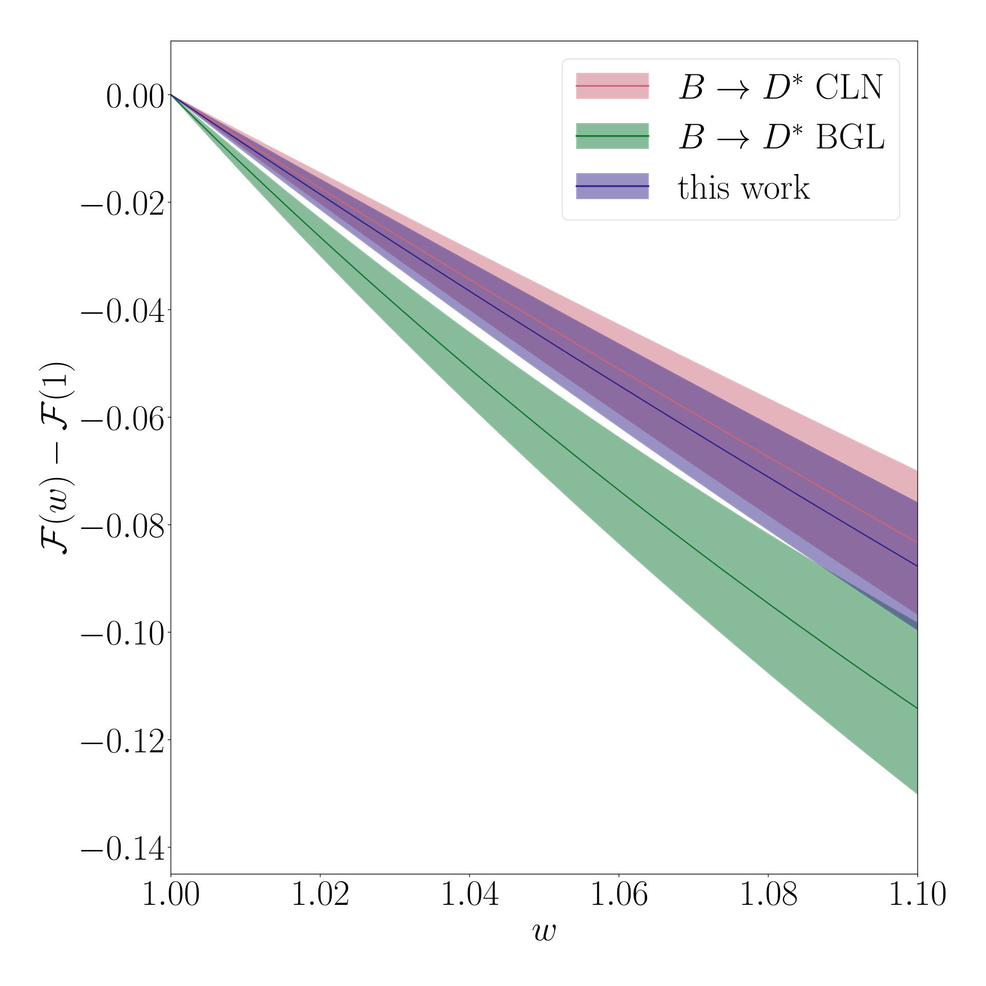
Here we find a value for the slope of

\frac{d\mathcal{F}^{B_{s}\to D_{s}^{*}}(w)}{dw}\Big|_{w=1}=-0.94\pm 0.15,

(62)

which we determine using a simple finite difference method. This is consistent with the slope for ${B\to D^{*}}$ determined from the CLN parameters extracted from experimental data including light cone sum rule constraints in Bigi et al. 2017b of $d\mathcal{F}^{B\to D^{*}}_{\mathrm{CLN}}(w)/dw|_{w=1}=-0.84(16)$ , where we have estimated the uncertainty from the uncertainties of the CLN parameters in Bigi et al. 2017b excluding correlations.

In Figure 16 we have plotted $\mathcal{F}(w)-\mathcal{F}(1)$ against $w$ where we see the difference between our results for the slope of $\mathcal{F}(w)$ near zero recoil for $B_{s}\to D_{s}^{*}$ compared to the slope computed from CLN and BGL fits to $B\to D^{*}$ experimental data in Bigi et al. 2017b. Note that our result for the slope is $\approx 2.5\sigma$ from the slope computed from the BGL fit, which we would expect to be similar for both $B\to D^{*}$ and $B_{s}\to D_{s}^{*}$ based on the small expected size of $SU(3)_{\mathrm{flavor}}$ breaking effects Bordone et al. 2020b.

VII LFUV Observables and Impact of New Physics Couplings

Figure 17:

d\Gamma/dq^{2}

\mathcal{A}_{FB}

and

\mathcal{A}_{\lambda_{\tau}}

for

\bar{B}_{s}^{0}\rightarrow D_{s}^{*+}\tau^{-}\bar{\nu}_{\tau}

in the SM and for the values of

g_{V_{R}}

and

g_{V_{L}}

given in Eq. (VII) from Bečirević et al. 2019.

d\Gamma/dq^{2}

is normalised to the total rate in the

\ell=\mu

case,

\Gamma_{\mu}

, and the

g_{V_{L}}

and

g_{V_{R}}

curves overlap. For

A_{F,B}

the SM and

g_{V_{L}}

curves overlap and for

A_{\lambda_{\tau}}

all three curves overlap. Note that here we do not include the contribution of

\delta_{\mathrm{EM}}

to the uncertainty.

In this section we study the impact of new physics (NP) couplings on observables in $B_{s}\to D_{s}^{*}$ decay. We do this by extending the analysis performed in Harrison et al. 2020b, where the NP couplings extracted from fits to $R(D)$ and $R(D^{*})$ in Bečirević et al. 2019 were used to predict the variations of the relevant observables defined in Bečirević et al. 2019 away from their Standard Model (SM) values for the case of $B_{c}\to J/\psi\ell\bar{\nu}_{\ell}$ . For $B_{s}\to D_{s}^{*}$ the relevant observables are the same, specifically those defined in Eq. (V.2) as well as their integrated values and ratios given in Eq. (V.2) and Eq. (V.2) respectively for the SM couplings. We also compute here the value of the tauonic/muonic ratio, $R(D_{s}^{*})$ , for different values of new physics couplings. Following Harrison et al. 2020b, we consider nonzero values for $g_{V_{R}}$ and $g_{V_{L}}$ , the complex-valued NP couplings multiplying left and right handed NP vector currents additional to those present in the SM. Here, as in Bečirević et al. 2019 and Harrison et al. 2020b, we only take these couplings to modify the tauonic decay.

In the left hand plot of Figure 17 we plot the tauonic differential rate, normalised by the muonic rate, where we see that both the left and right handed NP vector currents increase the tauonic differential rate markedly. The corresponding values of $R^{g_{i}}(D_{s}^{*})$ for each NP coupling, together with the numerical values of $g_{V_{R}}$ and $g_{V_{L}}$ , are;

$\displaystyle g_{V_{R}}=$	$\displaystyle-0.01-i\,0.39;\,$
	$\displaystyle R^{g_{V_{R}}}(D_{s}^{*})=0.2912(71)_{\mathrm{latt}}(40)_{\mathrm{EM}},$
$\displaystyle g_{V_{L}}=$	$\displaystyle\,0.07-i\,0.16;\,$
	$\displaystyle R^{g_{V_{L}}}(D_{s}^{*})=0.2915(71)_{\mathrm{latt}}(40)_{\mathrm{EM}}.$	(63)

These values are both larger than our SM value given in Eq. (44) and are both consistent with the HFLAV average experimental value for $R(D^{*})=0.295(14)$ Amhis et al. 2019.

The middle and right hand plots in Figure 17 show $\mathcal{A}_{FB}$ and $\mathcal{A}_{\lambda_{\tau}}$ respectively. Here we see that only $\mathcal{A}_{FB}$ , the forward-backward asymmetry of the final state tau lepton, is sensitive to changes in $g_{V_{R}}$ , only. As expected modifications to the left handed current do not result in a change away from the SM. For $\mathcal{A}_{\lambda_{\tau}}$ neither $g_{V_{R}}$ or $g_{V_{L}}$ produce any change. The integrated observables and ratios for these quantities are given in Table 16 and Table 17 respectively, where we repeat the SM results given in Table V.2 and Table V.2 for reference. Note that these are all within $1\sigma$ of the equivalent quantities computed for $B_{c}\to J/\psi\ell\bar{\nu}_{\ell}$ in Harrison et al. 2020b.

Table 16: Integrated angular variables defined in Bečirević et al. 2019 for the NP couplings given in Eq. (VII).

	SM	$g_{V_{R}}$	$g_{V_{L}}$
$\langle\mathcal{A}_{\lambda_{\tau}}\rangle$	0.520(12)	0.520(12)	0.520(12)
$\langle F^{D_{s}^{*}}_{L}$	0.440(16)	0.441(16)	0.440(16)
$\langle\mathcal{A}_{FB}\rangle$	-0.092(24)	-0.033(18)	-0.092(24)

Table 17: LFUV ratios defined in Bečirević et al. 2019 for the NP couplings given in Eq. (VII). Note that as expected from the form of the SM current, a modification to the left handed vector current does not change any of these ratios away from their SM values.

	SM	$g_{V_{R}}$	$g_{V_{L}}$
$R(\mathcal{A}_{\lambda_{\tau}})$	0.524(12)	0.524(12)	0.524(12)
$R(F_{L}^{J/\psi})$	0.878(18)	0.880(18)	0.878(18)
$R(\mathcal{A}_{FB})$	0.345(56)	0.126(57)	0.345(56)

VIII Conclusions

We have extended the heavy-HISQ methods of Harrison et al. 2020a to compute the four form factors, $A_{0}(q^{2})$ , $A_{1}(q^{2})$ , $A_{2}(q^{2})$ and $V(q^{2})$ , for $B_{s}\to D_{s}^{*}\ell\bar{\nu}_{\ell}$ across the full kinematic range of the decay for the first time using lattice QCD. As in Harrison et al. 2020a our calculation uses the HISQ action for all quarks, allowing us to normalise the lattice weak current operators that couple the $b$ and $c$ quarks fully nonperturbatively. We have included with this work the complete set of parameters and their correlations needed to reconstruct our form factors, which are expected to be useful in upcoming improved analyses by the LHCb experiment.

Using these form factors we have presented the first computation in lattice QCD of the total decay rate to each of the three different final state leptons, as well as the tauonic/muonic ratio. We find (repeating Sections V.1, V.1, V.1 and 44)

$\displaystyle\frac{\Gamma(B_{s}^{0}\to D_{s}^{*-}e^{+}{\nu}_{e})}{\|\eta_{\mathrm{EW}}V_{cb}\|^{2}}=$	$\displaystyle 2.07(17)_{\mathrm{latt}}(2)_{\mathrm{EM}}\times 10^{13}~\mathrm{s}^{-1}$
$\displaystyle\frac{\Gamma(B_{s}^{0}\to D_{s}^{*-}\mu^{+}{\nu}_{\mu})}{\|\eta_{\mathrm{EW}}V_{cb}\|^{2}}=$	$\displaystyle 2.06(16)_{\mathrm{latt}}(2)_{\mathrm{EM}}\times 10^{13}~\mathrm{s}^{-1}$
$\displaystyle\frac{\Gamma(B_{s}^{0}\to D_{s}^{*-}\tau^{+}{\nu}_{\tau})}{\|\eta_{\mathrm{EW}}V_{cb}\|^{2}}=$	$\displaystyle 5.14(37)_{\mathrm{latt}}(5)_{\mathrm{EM}}\times 10^{12}~\mathrm{s}^{-1}$
$\displaystyle R(D_{s}^{*})=$	$\displaystyle 0.2490(60)_{\mathrm{latt}}(35)_{\mathrm{EM}}.$	(64)

where the full error budget for these quantities is given in Table 14. Note that we have included an uncertainty in $R(D_{s}^{*})$ to allow for long-distance QED corrections that could differ between the $\tau$ and $\mu$ cases. These QED effects must be addressed in future calculations in order to produce results with reliable percent-level uncertainties.

Since the current experimental average for $R(D^{*})$ is causing some tension with the SM, we have considered the impact of NP scenarios using our form factors (Section VII), and illustrated how a modified left or right handed vector current consistent with measurements of $B\to D^{(*)}$ might show up in $B_{s}\to D_{s}^{*}$ decay. We have shown that these NP currents result in a modified value of $R(D_{s}^{*})$ which is larger than in the SM and is within $\approx 0.6\sigma$ of the current experimental average value of $R(D^{*})$ .

We have also computed the ratio of total SM rates for $B_{s}\to D_{s}$ and $B_{s}\to D_{s}^{*}$ . We find (repeating Eq. 52)

\frac{\Gamma(B^{0}_{s}\to D_{s}^{-}\mu^{+}\nu_{\mu})}{\Gamma(B_{s}^{0}\to D_{s}^{*-}\mu^{+}\nu_{\mu})}=0.443(40)_{\mathrm{latt}}(4)_{\mathrm{EM}}

(65)

which is in good agreement with the experimental value from LHCb Aaij et al. 2020a. We give the forward-backward asymmetry of the final state lepton, the lepton polarisation asymmetry and the longitudinal polarisation fraction in Eq. (V.2).

We have compared the normalised differential decay rate, $(1/\Gamma)d\Gamma/dq^{2}$ , computed using our form factors to the recent measurement of the shape of the decay by LHCb. We find that the measurement is broadly consistent with our computed shape, showing only very mild tension which can be seen to originate from a single $w$ bin. We have also used our results to determine the SM CLN parameters $\rho^{2}$ , $R_{0}(1)$ , $R_{1}(1)$ , $R_{2}(1)$ and $h_{A_{1}}(1)$ for $B_{s}\to D_{s}^{*}$ . The value of the slope of $h_{A_{1}}(w)$ , $\rho^{2}$ , measured by LHCb for $B_{s}\to D_{s}^{*}$ is found to be in good agreement with our computed value, while our values for the other parameters are seen to be consistent with values for the corresponding parameters for $B\to D^{*}$ .

Finally, we have used our result together with the reconstructed experimentally measured differential decay rate, parameterised using both the CLN and BGL schemes, to compute a value of $|V_{cb}|$ . We find the value computed in this way using lattice results across the full kinematic range is consistent with that computed using lattice input for only $h_{A_{1}}(1)$ . Our values for $|V_{cb}|$ computed using experimental results parameterised in the CLN and BGL schemes respectively are given in Eqs. 58 and 58. For $|V_{cb}|$ we take the average of their central values, with the larger of the two errors, to find (repeating Eq. (60))

|V_{cb}|=42.2(1.5)_{\mathrm{latt}}(1.7)_{\mathrm{exp}}(0.4)_{\mathrm{EM}}\times 10^{-3}.

(66)

This value is not yet accurate enough to resolve the tension between inclusive and exclusive (using $B\rightarrow D^{*}$ at zero recoil) values for $V_{cb}$ . Note that here, if binned experimental data for the differential rate was available, $|V_{cb}|$ could be determined by comparing our lattice results directly to experiment in a joint fit, without the need to use a parameterisation scheme.

Such a model-independent determination of $|V_{cb}|$ using $B_{s}\to D_{s}^{*}$ would require a reduction in uncertainty by a factor of $\approx 3$ in order to be competitive. Such a reduction in the uncertainty of our form factor results is feasible and may be achieved by working on ‘exafine’ lattices with lattice spacings $\approx 0.03\mathrm{fm}$ , allowing us to work directly at the physical $b$ quark mass, as well as by including additonal configurations to reduce statistical uncertainties at other values of the lattice spacing, as discussed in Section V.4.

Our work paves the way for the calculation of form factors for $B\rightarrow D^{*}$ decay across the full range of $q^{2}$ . This would also allow a direct determination of $|V_{cb}|$ from unfolded experimental results binned in $q^{2}$ , reducing the reliance on extrapolation to the zero recoil point.

Acknowledgements

We are grateful to the MILC collaboration for the use of their configurations and code. We thank C. Bouchard, B. Colquhoun, J. Koponen, P. Lepage, E. McLean and C. McNeile for useful discussions. Computing was done on the Cambridge service for Data Driven Discovery (CSD3), part of which is operated by the University of Cambridge Research Computing on behalf of the DIRAC HPC Facility of the Science and Technology Facilities Council (STFC). The DIRAC component of CSD3 was funded by BEIS capital funding via STFC capital grants ST/P002307/1 and ST/R002452/1 and STFC operations grant ST/R00689X/1. DiRAC is part of the national e-infrastructure. We are grateful to the CSD3 support staff for assistance. Funding for this work came from the UK Science and Technology Facilities Council grants ST/L000466/1 and ST/P000746/1.

Appendix A Lattice Results

Here, in Tables 18, 19, 20 and 21, we give the lattice results for the form factors, including renormalisation factors, which were extracted from the matrix elements in Eq. (13) resulting from the fits discussed in Section III.

Table 18: Lattice form factor results for set 1.

ak

here is the value of the

x

and

y

components of the lattice momentum for the

D_{s}^{*}

ak

is calculated from the corresponding twist in Table 4.

$am_{h}$	$ak$	$A_{0}$	$A_{1}$	$A_{2}$	$V$
0.65	0.0	$-$	0.9261(53)	$-$	$-$
	0.0358913	0.90(13)	0.9251(54)	1.1(2.0)	1.09(48)
	0.0717826	0.898(68)	0.9226(57)	1.21(83)	1.21(22)
	0.107674	0.893(48)	0.9183(61)	1.22(58)	1.23(15)
	0.143565	0.882(38)	0.9120(67)	1.24(50)	1.23(12)
	0.179456	0.867(33)	0.9037(76)	1.26(48)	1.22(10)
0.725	0.0	$-$	0.9277(54)	$-$	$-$
	0.0358913	0.92(14)	0.9267(55)	0.8(2.3)	1.10(49)
	0.0717826	0.913(71)	0.9242(58)	1.01(71)	1.22(22)
	0.107674	0.907(50)	0.9199(62)	1.04(42)	1.24(15)
	0.143565	0.897(40)	0.9136(68)	1.06(33)	1.24(12)
	0.179456	0.882(35)	0.9052(78)	1.07(30)	1.23(10)
0.8	0.0	$-$	0.9299(56)	$-$	$-$
	0.0358913	0.93(14)	0.9289(57)	0.7(2.7)	1.12(49)
	0.0717826	0.930(75)	0.9264(59)	0.91(76)	1.24(22)
	0.107674	0.924(53)	0.9220(63)	0.95(40)	1.26(16)
	0.143565	0.913(43)	0.9157(70)	0.97(28)	1.25(12)
	0.179456	0.898(37)	0.9073(80)	0.98(23)	1.24(11)

Table 19: Lattice form factor results for set 2.

ak

here is the value of the

x

and

y

components of the lattice momentum for the

D_{s}^{*}

ak

is calculated from the corresponding twist in Table 4.

$am_{h}$	$ak$	$A_{0}$	$A_{1}$	$A_{2}$	$V$
0.427	0.0	$-$	0.908(12)	$-$	$-$
	0.0524832	0.89(18)	0.906(13)	1.6(1.7)	1.26(56)
	0.104966	0.87(10)	0.896(15)	1.07(96)	1.23(31)
	0.15745	0.824(79)	0.879(18)	0.97(94)	1.19(25)
	0.209933	0.768(75)	0.857(23)	1.0(1.3)	1.13(24)
	0.262416	0.705(78)	0.831(32)	1.2(2.8)	1.06(24)
0.525	0.0	$-$	0.904(13)	$-$	$-$
	0.0524832	0.92(20)	0.903(13)	1.9(1.7)	1.26(58)
	0.104966	0.89(11)	0.893(15)	1.13(60)	1.24(33)
	0.15745	0.851(87)	0.875(18)	0.97(46)	1.20(27)
	0.209933	0.792(83)	0.852(24)	0.91(51)	1.14(25)
	0.262416	0.727(86)	0.825(33)	0.90(69)	1.07(26)
0.65	0.0	$-$	0.900(13)	$-$	$-$
	0.0524832	0.96(22)	0.898(14)	2.3(2.2)	1.28(61)
	0.104966	0.94(12)	0.888(15)	1.24(63)	1.27(35)
	0.15745	0.891(98)	0.870(19)	1.03(37)	1.22(28)
	0.209933	0.829(93)	0.847(25)	0.94(33)	1.17(27)
	0.262416	0.760(97)	0.821(35)	0.89(37)	1.09(28)
0.8	0.0	$-$	0.896(14)	$-$	$-$
	0.0524832	1.02(25)	0.895(14)	2.6(2.8)	1.32(64)
	0.104966	0.99(14)	0.884(16)	1.36(78)	1.31(37)
	0.15745	0.94(11)	0.866(20)	1.10(42)	1.26(30)
	0.209933	0.88(11)	0.843(26)	0.99(31)	1.20(29)
	0.262416	0.80(11)	0.817(36)	0.93(30)	1.13(30)

Table 20: Lattice form factor results for set 3.

ak

here is the value of the

x

and

y

components of the lattice momentum for the

D_{s}^{*}

ak

is calculated from the corresponding twist in Table 4.

$am_{h}$	$ak$	$A_{0}$	$A_{1}$	$A_{2}$	$V$
0.5	0.0	$-$	0.8810(73)	$-$	$-$
	0.0585768	0.963(62)	0.8705(79)	1.00(54)	1.42(19)
	0.117154	0.907(40)	0.839(11)	0.83(18)	1.31(13)
	0.17573	0.818(43)	0.792(18)	0.75(14)	1.20(14)
	0.234307	0.714(59)	0.740(32)	0.66(21)	1.08(18)
	0.292884	0.620(87)	0.676(68)	0.45(45)	0.97(30)
0.65	0.0	$-$	0.8684(75)	$-$	$-$
	0.0585768	1.034(73)	0.8584(82)	1.00(74)	1.47(20)
	0.117154	0.976(48)	0.828(11)	0.86(24)	1.36(14)
	0.17573	0.881(51)	0.782(18)	0.79(16)	1.24(14)
	0.234307	0.767(69)	0.731(33)	0.72(17)	1.11(20)
	0.292884	0.66(10)	0.668(70)	0.59(27)	1.00(33)
0.8	0.0	$-$	0.8580(77)	$-$	$-$
	0.0585768	1.109(84)	0.8485(84)	0.96(92)	1.54(21)
	0.117154	1.048(55)	0.819(11)	0.88(30)	1.41(14)
	0.17573	0.948(59)	0.774(19)	0.83(20)	1.28(15)
	0.234307	0.823(81)	0.723(33)	0.78(19)	1.15(22)
	0.292884	0.70(12)	0.660(72)	0.67(26)	1.04(36)

Table 21: Lattice form factor results for set 4.

ak

here is the value of the

x

and

y

components of the lattice momentum for the

D_{s}^{*}

ak

is calculated from the corresponding twist in Table 4.

$am_{h}$	$ak$	$A_{0}$	$A_{1}$	$A_{2}$	$V$
0.5	0.0	$-$	0.9244(90)	$-$	$-$
	0.0356761	0.87(25)	0.9240(92)	8(35)	1.37(93)
	0.0713522	0.88(12)	0.9213(98)	6(25)	1.27(44)
	0.107028	0.874(90)	0.917(11)	20(65)	1.27(33)
	0.142704	0.859(76)	0.911(12)	-7(22)	1.25(27)
	0.178381	0.840(69)	0.904(13)	-1.9(7.4)	1.22(24)
0.65	0.0	$-$	0.9272(98)	$-$	$-$
	0.0356761	0.90(29)	0.927(10)	1.7(4.0)	1.4(1.0)
	0.0713522	0.91(14)	0.924(11)	1.2(1.5)	1.28(47)
	0.107028	0.90(10)	0.920(12)	1.2(1.1)	1.28(35)
	0.142704	0.884(88)	0.914(13)	1.14(97)	1.26(29)
	0.178381	0.865(80)	0.906(15)	1.13(97)	1.23(26)
0.8	0.0	$-$	0.931(10)	$-$	$-$
	0.0356761	0.93(33)	0.931(11)	1.7(5.6)	1.5(1.1)
	0.0713522	0.95(16)	0.928(12)	1.2(1.6)	1.31(50)
	0.107028	0.94(12)	0.923(13)	1.12(84)	1.31(37)
	0.142704	0.92(10)	0.917(14)	1.07(61)	1.28(30)
	0.178381	0.900(92)	0.909(16)	1.03(53)	1.25(27)

Appendix B Reconstructing the Fit

Our parameterisation of the form factors for $B_{s}\to D_{s}^{*}$ in the continuum limit is given by Eq. (36). It consists of a pole factor with no uncertainty and a polynomial in $z$ for which the coefficients with their uncertainties are given in Table 13. In this section we give the correlations between the $z$ -expansion coefficients which are necessary for reconstructing our results explicitly, as well as instructions for using the included ancillary files to load the $z$ -expansion parameters together with their correlations automatically into python Van Rossum and Drake 2009.

The correlation between two coefficients is defined in the usual way as

\mathrm{Corr}(X,Y)=\frac{\langle(\bar{X}-X)(\bar{Y}-Y)\rangle}{\sqrt{\sigma^{2}(X)\sigma^{2}(Y)}}

(67)

where $\sigma^{2}(X)$ is the variance of $X$ and $\bar{X}$ is the mean of $X$ . The values are tabulated in Tables 22, 23, 24, 25, 26, 27, 28, 29, 30 and 31.

In this calculation and in the ancillary files we use the gvar python package to track and propagate correlations. Included in the ancillary files are two text files; CORRELATIONS.txt contains a dictionary including the means and variances of the $z$ -expansion parameters on the first line and a dictionary detailing the correlations between these parameters on the second line, CHECKS.txt contains arrays of $q^{2}$ values and form factor mean and standard deviation values at the corresponding values of $q^{2}$ . This file is used by the python script load_fit.py as a simple check that the fit has been loaded correctly. Running python load_fit.py will load the parameters from CORRELATIONS.txt and compare values computed at hard coded intervals in $q^{2}$ to those in CHECKS.txt which were computed as part of this work. Running python load_fit.py will also produce some simple plots of the form factors across the full $q^{2}$ range. We have tested load_fit.py using Python 3.7.5 Van Rossum and Drake 2009, gvar 9.2.1 Lepage gvar, numpy 1.18.2 van der Walt et al. 2011 and matplotlib 3.1.2 Hunter 2007.

Table 22: Correlation matrix for

z

-expansion coefficients of

A0

$\sigma^{2}$	$a_{0}^{A0}$	$a_{1}^{A0}$	$a_{2}^{A0}$	$a_{3}^{A0}$
$a_{0}^{A0}$	1.0	-0.3781	-0.007023	-0.004275
$a_{1}^{A0}$	-0.3781	1.0	-0.1681	0.00345
$a_{2}^{A0}$	-0.007023	-0.1681	1.0	-0.002318
$a_{3}^{A0}$	-0.004275	0.00345	-0.002318	1.0

Table 23: Correlation matrix for

z

-expansion coefficients of

A0

and

A1

$\sigma^{2}$	$a_{0}^{A1}$	$a_{1}^{A1}$	$a_{2}^{A1}$	$a_{3}^{A1}$
$a_{0}^{A0}$	0.2776	-0.02225	0.1044	0.01322
$a_{1}^{A0}$	0.04791	0.0006896	-0.2142	-0.02751
$a_{2}^{A0}$	-0.01723	0.03742	0.0506	-0.003768
$a_{3}^{A0}$	0.003371	-0.008893	0.0279	0.006599

Table 24: Correlation matrix for

z

-expansion coefficients of

A0

and

A2

$\sigma^{2}$	$a_{0}^{A2}$	$a_{1}^{A2}$	$a_{2}^{A2}$	$a_{3}^{A2}$
$a_{0}^{A0}$	-0.3816	0.2939	-0.09207	-0.006694
$a_{1}^{A0}$	0.03317	-0.4783	0.1869	0.01545
$a_{2}^{A0}$	0.1246	-0.2087	-0.01677	0.004254
$a_{3}^{A0}$	0.005469	-0.001225	-0.03466	-0.004052

Table 25: Correlation matrix for

z

-expansion coefficients of

A0

and

V

$\sigma^{2}$	$a_{0}^{V}$	$a_{1}^{V}$	$a_{2}^{V}$	$a_{3}^{V}$
$a_{0}^{A0}$	-0.002394	-0.01266	-0.000435	-2.199e-05
$a_{1}^{A0}$	0.003344	0.01268	0.000509	2.598e-05
$a_{2}^{A0}$	-0.001888	0.003397	0.0003099	1.767e-05
$a_{3}^{A0}$	0.0001465	0.0001454	2.376e-05	1.374e-06

Table 26: Correlation matrix for

z

-expansion coefficients of

A1

$\sigma^{2}$	$a_{0}^{A1}$	$a_{1}^{A1}$	$a_{2}^{A1}$	$a_{3}^{A1}$
$a_{0}^{A1}$	1.0	-0.03043	-0.01583	-0.01588
$a_{1}^{A1}$	-0.03043	1.0	-0.3144	0.02958
$a_{2}^{A1}$	-0.01583	-0.3144	1.0	-0.09184
$a_{3}^{A1}$	-0.01588	0.02958	-0.09184	1.0

Table 27: Correlation matrix for

z

-expansion coefficients of

A1

and

A2

$\sigma^{2}$	$a_{0}^{A2}$	$a_{1}^{A2}$	$a_{2}^{A2}$	$a_{3}^{A2}$
$a_{0}^{A1}$	0.3327	-0.09657	0.066	0.01124
$a_{1}^{A1}$	0.4326	0.04303	-0.1541	-0.02324
$a_{2}^{A1}$	-0.3016	0.5087	0.485	0.05027
$a_{3}^{A1}$	-0.005564	-0.007639	0.1149	0.01492

Table 28: Correlation matrix for

z

-expansion coefficients of

A1

and

V

$\sigma^{2}$	$a_{0}^{V}$	$a_{1}^{V}$	$a_{2}^{V}$	$a_{3}^{V}$
$a_{0}^{A1}$	0.008341	0.009546	0.0007997	4.367e-05
$a_{1}^{A1}$	0.01089	0.02048	0.0008922	4.38e-05
$a_{2}^{A1}$	-0.000702	0.01654	0.0008034	4.176e-05
$a_{3}^{A1}$	-0.001079	0.0005229	1.918e-06	-2.31e-08

Table 29: Correlation matrix for

z

-expansion coefficients of

A2

$\sigma^{2}$	$a_{0}^{A2}$	$a_{1}^{A2}$	$a_{2}^{A2}$	$a_{3}^{A2}$
$a_{0}^{A2}$	1.0	-0.6033	0.1237	-0.001915
$a_{1}^{A2}$	-0.6033	1.0	-0.2094	0.01039
$a_{2}^{A2}$	0.1237	-0.2094	1.0	-0.07082
$a_{3}^{A2}$	-0.001915	0.01039	-0.07082	1.0

Table 30: Correlation matrix for

z

-expansion coefficients of

A2

and

V

$\sigma^{2}$	$a_{0}^{V}$	$a_{1}^{V}$	$a_{2}^{V}$	$a_{3}^{V}$
$a_{0}^{A2}$	0.01155	-0.025	-0.000755	-3.602e-05
$a_{1}^{A2}$	-0.002784	0.04492	0.001724	8.523e-05
$a_{2}^{A2}$	0.003861	-0.002808	0.0001025	7.013e-06
$a_{3}^{A2}$	0.0008794	4.2e-05	2.166e-05	1.227e-06

Table 31: Correlation matrix for

z

-expansion coefficients of

V

$\sigma^{2}$	$a_{0}^{V}$	$a_{1}^{V}$	$a_{2}^{V}$	$a_{3}^{V}$
$a_{0}^{V}$	1.0	-0.4502	0.0155	0.0007512
$a_{1}^{V}$	-0.4502	1.0	-0.1043	-0.003208
$a_{2}^{V}$	0.0155	-0.1043	1.0	-0.0001705
$a_{3}^{V}$	0.0007512	-0.003208	-0.0001705	1.0

Appendix C BGL Parameters and Unitarity Check

C.1 Conversion to BGL Scheme

We may also use our results to determine the parameters entering the BGL parameterisation. This allows us to check the unitarity constraints $\sum(a^{\mathrm{BGL}}_{n})^{2}\leq 1$ To do this we convert our form factors to the helicity basis, given by Cohen et al. 2018:

$\displaystyle g=$	$\displaystyle\frac{2}{M_{B_{s}}+M_{D_{s}^{*}}}V$
$\displaystyle f=$	$\displaystyle(M_{B_{s}}+M_{D_{s}^{*}})A_{1}$
$\displaystyle F_{1}=$	$\displaystyle\frac{M_{B_{s}}+M_{D_{s}^{}}}{M_{D_{s}^{}}}\Big[-\frac{2M_{B_{s}}^{2}\|{\vec{p}}^{\prime}\|^{2}}{(M_{B_{s}}+M_{D_{s}^{*}})^{2}}A_{2}$
	$\displaystyle-\frac{1}{2}(t-M_{B_{s}}^{2}+M_{D_{s}^{*}}^{2})A_{1}\Big]$
$\displaystyle F_{2}=$	$\displaystyle 2A_{0}$	(68)

where ${\vec{p}}^{\prime}$ is the $D_{s}^{*}$ spatial momentum in the $B_{s}$ rest frame. The BGL scheme then parameterises these form factors using the expansion in $z$ space,

F(t)=\frac{1}{P(t)\phi(t,t_{0})}\sum_{n=0}^{\infty}a^{\mathrm{BGL}}_{n}z(t,t_{0})^{n}

(69)

where the pole function $P_{i}$ is the same as we have defined in Eq. (24) and the outer functions, $\phi$ , are defined in Cohen et al. 2018. We use the resonance masses given in Cohen et al. 2018 in the pole functions $P_{i}$ . In order to compute the outer functions we use the values of $\chi_{L(T)}(\pm u)$ computed in Harrison et al. 2020a. We use our results to output form factor values in the helicity basis at a large number of $q^{2}$ values, which we subsequently fit using Eq. (69) truncated at $n=3$ . Our results, expressed in terms of the BGL parameterisation, are given in Table 32, together with the unitarity bounds which we find to be far from saturation.

Table 32: BGL parameters computed by converting the physical continuum results computed using Eq. (25) to the BGL scheme, Eq. (69).

	$a^{\mathrm{BGL}}_{0}$	$a^{\mathrm{BGL}}_{1}$	$a^{\mathrm{BGL}}_{2}$	$a^{\mathrm{BGL}}_{3}$	$\sum(a^{\mathrm{BGL}}_{n})^{2}$
$F_{1}$	0.002402(90)	-0.0018(44)	-0.041(97)	0.04(82)	0.003(74)
$F_{2}$	0.0384(21)	-0.077(45)	-0.25(42)	0.0(1.0)	0.07(21)
$f$	0.01420(53)	-0.019(14)	-0.0(0.2)	0.0(1.0)	0.00055(84)
$g$	0.0300(33)	0.0(0.08)	-0.04(54)	0.0(1.0)	0.002(41)

C.2 Comparison to $B\to D^{*}$ BGL Coefficients

As well as checking that the unitarity constraints are satisfied by the BGL parameters for $B_{s}\to D_{s}^{*}$ it is also useful and interesting to reparameterise our results using the BGL scheme for $B\to D^{*}$ . This allows us to compare our results to those for $B\to D^{*}$ , and also allows for our results to be more readily incorporated into analyses which assume $SU(3)_{\mathrm{flav}}$ symmetry.

The BGL coefficients are sensitive to the meson masses through the outer functions and through the definition of $z(q^{2},t_{0},t_{+})$ . In order to reparameterise our results using the BGL scheme for $B\to D^{*}$ we first convert our results to the helicity basis, using the $B_{s}$ and $D_{s}^{*}$ masses (as in Eq. (C.1)), and then fit these to the BGL parameterisation for $B\to D^{*}$ , in which $z(q^{2},t_{0},t_{+})$ and the outer functions are computed using the $B$ and $D^{*}$ masses. In order to compare to the BGL coefficients for $B\to D^{*}$ determined in Bigi et al. 2017c; Bigi et al. 2017b we use the masses and values of $\chi_{L(T)}(\pm u)$ given in Tables IV and III of Bigi et al. 2017c. Bigi et al. 2017c and Bigi et al. 2017b both use the same definitions for the outer functions, given in Boyd et al. 1997, which we also use here, as well as choosing $t_{0}=t_{-}$ . Note that these definitions differ from those used in Appendix C.1, from Cohen et al. 2018, where the $t_{+}$ is given by the true pair production threshold in each channel (e.g. the threshold for $BD$ production for the vector channel and the threshold for $B^{*}D$ production for the axial-vector and pseudoscalar channels), whereas in Boyd et al. 1997 and Bigi et al. 2017c; Bigi et al. 2017b it is taken to be $(M_{D^{*}}+M_{B})^{2}$ for all channels. Note also that since our results for $B_{s}\to D_{s}^{*}$ satisfy the kinematical constraint Eq. (33), involving the $B_{s}$ and $D_{s}^{*}$ masses, the equivalent constraint for $B\to D^{*}$ will not be satisfied and so must be imposed. We must also impose the constraint $F_{1}(q^{2}_{\mathrm{max}})=(M_{B}-M_{D^{*}})f(q^{2}_{\mathrm{max}})$ which will not otherwise be satisfied. We impose these constraints explicitly by using them to fix the zeroth-order coefficients of $F_{2}$ and $F_{1}$ .

We use a BGL parameterisation including up to $z^{2}$ terms for $f,~F_{1}$ and $g$ , and up to $z$ for $F_{2}$ . The coefficients are given in Table 33, where we see that our results are consistent with the BGL parameters for $B\to D^{*}$ . The correlation matrix for our results in this parameterisation scheme is given in Table 34. We conclude that there is no significant effect on the form factors evident in our results with a strange spectator quark compared to those with an up/down one.

Table 33: BGL parameters for our results determined using the BGL parameterisation for

B\to D^{*}

, compared to the BGL parameters extracted from experimental data, lattice results and light cone sum rules for

B\to D^{*}

in Bigi et al. 2017b.

BGL Fit:	This work, $B_{s}\to D_{s}^{*}$	$B\to D^{*}$ Bigi et al. 2017b
$a_{0}^{f}$	0.01258(47)	0.01224(18)
$a_{1}^{f}$	-0.008(15)	-0.052(+27,-15)
$a_{2}^{f}$	-0.03(22)	1.0(+0,-5)
$a_{1}^{F_{1}}$	0.00009(402)	-0.0070(+54,-52)
$a_{2}^{F_{1}}$	-0.066(61)	0.089(+96,-100)
$a_{0}^{g}$	0.0339(37)	0.0289(+57,-37)
$a_{1}^{g}$	0.005(100)	0.08(+8,-22)
$a_{2}^{g}$	-0.005(315)	-1.0(+2.0,-0)
$a_{1}^{F_{2}}$	0.0108(50)	$-$

Table 34: Correlation matrix for our BGL parameters determined using the BGL parameterisation for

B\to D^{*}

, given in Table 33.

	$a_{0}^{f}$	$a_{1}^{f}$	$a_{2}^{f}$	$a_{1}^{F_{1}}$	$a_{2}^{F_{1}}$	$a_{0}^{g}$	$a_{1}^{g}$	$a_{2}^{g}$	$a_{1}^{F_{2}}$
$a_{0}^{f}$	1.0	-0.097	0.057	-0.192	0.031	0.008	0.011	0.006	0.127
$a_{1}^{f}$		1.0	-0.546	0.191	-0.204	0.014	0.011	-0.043	-0.033
$a_{2}^{f}$			1.0	-0.051	0.007	-0.009	0.024	0.081	-0.059
$a_{1}^{F_{1}}$				1.0	-0.737	-0.002	0.036	-0.016	0.177
$a_{2}^{F_{1}}$					1.0	-0.001	-0.043	0.019	0.414
$a_{0}^{g}$						1.0	-0.382	0.006	0.002
$a_{1}^{g}$							1.0	-0.087	0.014
$a_{2}^{g}$								1.0	0.007
$a_{1}^{F_{2}}$									1.0

Appendix D Stability of our Form Factors Under Variations of the Fit

D.1 Variations of Correlator Fits

In Figure 18 and Figure 19 we show the variation of the form factors $A_{0}$ and $A_{2}$ , evaluated at $q^{2}=1~\mathrm{GeV}^{2},5~\mathrm{GeV}^{2},10~\mathrm{GeV}^{2}$ , as in Figure 6. In these plots we see that these form factors do not change significantly as a result of varying the correlator fit inputs.

Figure 18: As for Figure 6 showing the stability of the form factor

A_{0}

evaluated at

q^{2}=1~\mathrm{GeV}^{2},5~\mathrm{GeV}^{2},10~\mathrm{GeV}^{2}

Figure 19: As for Figure 6 showing the stability of the form factor

A_{2}

evaluated at

q^{2}=1~\mathrm{GeV}^{2},5~\mathrm{GeV}^{2},10~\mathrm{GeV}^{2}

D.2 Order of Expansion

We also investigate the effects of including fewer $z$ terms in Eq. (25) as well as fewer $am_{c}$ , $am_{h}$ and $2\Lambda_{QCD}/M_{\eta_{h}}$ terms in Eq. (26). Figure 20 gives the total width, as well as values of the form factors at several values of $q^{2}$ , obtained using these variations, where we see that our results are insensitive to the removal of the highest order terms. We also investigate the effect of increasing or decreasing the prior widths of the parameters $b_{n}^{ijk}$ in Eq. (26) by a factor of 2. These results are also shown in Figure 20 where, as in Harrison et al. 2020a, we see only a very small effect on the central values of our results. .

Figure 20: Plot showing the stability of the total rate for

B_{s}^{0}\to D_{s}^{*-}\mu^{+}{\nu}_{\mu}

considering lower order truncations of

z

-expansion, discretisation and heavy mass dependent terms in Eq. (25) and Eq. (26).

\mathcal{O}({n_{1}},{n_{2}},{n_{3}},{n_{4}})

corresponds to the result including terms of highest order

\mathcal{O}((2\Lambda/M_{\eta_{h}})^{n_{1}},(am_{c})^{2n_{2}},(am_{h})^{2n_{3}},z^{n_{4}})

. The vertical black line is our final result, corresponding to

\mathcal{O}({3},{3},{3},{3})

, and the grey band is its uncertainty. We also include variations in which we multiply our prior widths either by a factor of 2 or 0.5, labelled as

0(\sigma)\rightarrow 0(\sigma\times 2)

and

0(\sigma)\rightarrow 0(\sigma/2)

respectively. Our result for the total rate is very stable to these variations. Note that here we do not include the contribution of

\delta_{\mathrm{EM}}

to the uncertainty. We also include similar plots for the form factors, evaluated at

q^{2}=1~\mathrm{GeV}^{2},5~\mathrm{GeV}^{2},10~\mathrm{GeV}^{2}

plotted in green, red and blue respectively.

D.3 Variation of Pole Term

Figure 21: Magnitude of the

\mathcal{O}(z)

coefficient,

a_{1}

, for each form factor plotted against the number of poles included in Eq. (24). The prior widths on the

b_{n}^{ijk}

are scaled according to the number of poles, see text. Note that the maximum number of poles included for

A_{0}

is 3. The black crosses and error bars give the total width for the

\ell=\mu

case,

\Gamma/|\eta_{\mathrm{EW}}V_{cb}|^{2}

, determined from that fit, using the right-hand

y

axis. The grey band corresponds to our final result for the total width using

N_{\mathrm{poles}}=4

, and prior values for

b_{n}^{ijk}

0(1)

. This shows how the different coefficients as a function of

N_{\mathrm{poles}}

give a very stable result for the total width. Note that here we do not include the contribution of

\delta_{\mathrm{EM}}

to the uncertainty in

\Gamma/|\eta V_{cb}|^{2}

The pole function Eq. (24) includes the effects of subthreshold $b\bar{c}$ resonances in $q^{2}$ . These begin at the square of the $B_{c}$ mass, $(6.275\mathrm{GeV})^{2}$ , significantly above the maximum physical value of $q^{2}_{\mathrm{max}}\approx(3.25\mathrm{GeV})^{2}$ . As such we do not expect the exact positions or number of poles to have a large effect on the fits, although the choice of the number of poles to include will act as a normalisation, changing the magnitude of the coefficients $a_{n}$ appearing in Eq. (25). Here we investigate the effect of including fewer poles in Eq. (24) by repeating our analysis including only the first $N_{\mathrm{poles}}$ resonances listed in Table 12.

We take a prior width on the $z$ -expansion coefficients of $5.0-N_{\mathrm{poles}}$ . We are able to obtain a good fit, with $\chi^{2}/\mathrm{dof}\approx 0.1$ in all cases. Since there are only 3 poles for $A_{0}$ expected below $t_{+}$ , we include only 3 poles for that form factor even in the $N_{\mathrm{poles}}$ case.

Figure 21 shows these results, plotting against the left-hand $y$ -axis the magnitude of the coefficient corresponding to the order $z$ term, $a_{1}$ , coming from the fits as a function of the number of poles included. Results are given for each form factor. We see that as we include fewer poles, increasingly large $z$ -expansion coefficients are needed partly in order to account for the removal of physical $q^{2}$ dependence from missing poles but also because of the normalisation change.

D.4 Inclusion of Outer Functions

Table 35: BGL parameters computed using the full BGL scheme including outer functions for the physical continuum extrapolation using Eq. (70). Note that these values are in good agreement with those computed by converting the physical continuum results computed using Eq. (25) to the BGL scheme, given in Table 32

	$a^{\mathrm{BGL^{\prime}}}_{0}$	$a^{\mathrm{BGL^{\prime}}}_{1}$	$a^{\mathrm{BGL^{\prime}}}_{2}$	$a^{\mathrm{BGL^{\prime}}}_{3}$	$\sum(a^{\mathrm{BGL^{\prime}}}_{n})^{2}$
$F_{1}$	0.00235(10)	-0.0058(63)	-0.04(13)	-0.31(91)	0.10(56)
$F_{2}$	0.0357(33)	-0.122(79)	-0.20(87)	0.0(1.0)	0.06(34)
$f$	0.01388(62)	-0.017(26)	-0.10(54)	0.0(1.0)	0.01(11)
$g$	0.0329(57)	-0.03(11)	0.01(99)	0.0(1.0)	0.002(21)

In order to investigate the effect of excluding the outer functions from Eq. (25) we consider using the BGL parameterisation described in Appendix C.1 for the extrapolation to the physical point of Section IV.1. In order to do this, we first convert our lattice data for the form factors to the helicity basis given in Eq. (C.1). To evaluate the outer functions $\phi$ , defined in Cohen et al. 2018, as we vary the heavy mass we must evaluate the function $\chi_{L(T)}(\pm u_{h})$ , defined in Boyd et al. 1997, at different values of $u_{h}$ . As in Harrison et al. 2020a we take $u_{b}=0.33$ , $m_{b}^{\mathrm{pole}}=4.78$ and $\alpha_{s}=0.22$ . We use $u_{h}=u_{b}\times M_{\eta_{b}}/M_{\eta_{h}}$ to approximate the heavy mass dependence of $u_{h}$ , as well as using $m_{h}^{\mathrm{pole}}=m_{b}^{\mathrm{pole}}\times M_{\eta_{h}}/M_{\eta_{b}^{\mathrm{phys}}}$ . Our BGL fit function then has the form

F(t)=\frac{1}{P(t)\phi(t,t_{0})}\sum_{n=0}^{\infty}a^{\mathrm{BGL^{\prime}}}_{n}z(t,t_{0})^{n}

(70)

with

a^{\mathrm{BGL^{\prime}}}_{n}=\sum_{j,k,l=0}^{3}b_{n}^{{}^{\prime}jkl}\Delta_{h}^{(j)}\left(\frac{am_{c}^{\mathrm{val}}}{\pi}\right)^{2k}\left(\frac{am_{h}^{\mathrm{val}}}{\pi}\right)^{2l}\mathcal{N}_{n}.

(71)

where $\mathcal{N}$ and $\Delta_{h}^{(j)}$ have the same definitions as in the main analysis discussed in Section IV.1. We take $t_{0}=t_{-}=q^{2}_{\mathrm{max}}$ , and use the same approximate form as in Section IV.1 for the variation of the pole masses with the heavy quark mass. We take the same priors as in Section IV.1 for the coefficients $b_{n}^{{}^{\prime}jkl}$ and for those entering $\mathcal{N}_{n}$ . In this fit we also impose the kinematical constraint at $q^{2}=0$ , which here takes the form $2F_{1}(0)-F_{2}(0)(M_{B_{s}}^{2}-M_{D_{s}^{*}}^{2})=0$ . Note that this is equivalent to the constraint $2M_{D_{s}^{*}}A_{0}(0)=(M_{D_{s}^{*}}+M_{H_{s}})A_{1}(0)+(M_{D_{s}^{*}}-M_{H_{s}})A_{2}(0)$ from the definitions of the helicity basis form factors given in Eq. (C.1). We also have, from the definitions Eq. (C.1), the additional condition that $F_{1}(q^{2}_{\mathrm{max}})=(M_{B_{s}}-M_{D_{s}^{*}})f(q^{2}_{\mathrm{max}})$ . We impose these conditions both at the physical point and on each lattice including a nuisance term as in Section IV.1. Note that here we neglect the running of $\alpha_{s}$ with heavy mass, allowing for this to be taken up elsewhere in the fit. The results of fitting our lattice data to Eq. (70) are given in Table 35, where we see that the BGL parameters from this fit are very close to those given in Table 32 which were computed from the continuum form factors extrapolated to the physical continuum using Eq. (25) without including outer functions. In both cases the unitarity bounds are far from saturation without the need to impose this constraint in our fits. This shows that the approach adopted here and in Harrison et al. 2020a, of excluding the outer functions from the physical continuum extrapolation, is consistent with including them.

The physical continuum form factors computed using Eq. (70) (converted to the $A_{0},A_{1},A_{2},V$ basis) are given in Figure 22, together with those computed using Eq. (25). The total rate computed using the outer functions is, for the $\ell=\mu$ case, $\Gamma^{\mathrm{BGL^{\prime}}}=1.88(20)_{\mathrm{latt}}(2)_{\mathrm{EM}}\times 10^{13}~\mathrm{s}^{-1}$ , compared to $\Gamma=2.06(16)_{\mathrm{latt}}(2)_{\mathrm{EM}}\times 10^{13}~\mathrm{s}^{-1}$ computed in Section V, again demonstrating that the exclusion of the outer functions during the extrapolation to the physical continuum point does not have any significant effect on our results.

In Figure 22 we also plot form factors resulting from performing the extrapolation in the HQET basis. The form factors in this basis are related to the form factors in the helicity basis by

$\displaystyle g=$	$\displaystyle\frac{h_{V}}{M_{B_{s}}\sqrt{r}}$
$\displaystyle f=$	$\displaystyle\sqrt{r}(1+w)h_{A_{1}}$
$\displaystyle F_{1}=$	$\displaystyle M_{B_{s}}^{2}\sqrt{r}(1+w)\left((w-r)h_{A_{1}}-(w-1)(rh_{A_{2}}+h_{A_{3}})\right)$
$\displaystyle F_{2}=$	$\displaystyle\frac{1}{\sqrt{r}}\left((1+w)h_{A_{1}}+(rw-1)h_{A_{2}}+(r-w)h_{A_{3}}\right),$	(72)

and for this extrapolation we use a simple form in powers of $w-1$ , which does not include any information about the pole terms:

F(t)=\sum_{n=0}^{\infty}a^{\mathrm{HQET}}_{n}(w-1)^{n}.

(73)

Here

a^{\mathrm{HQET}}_{n}=\sum_{j,k,l=0}^{3}b_{n}^{{}^{\prime\prime}jkl}\Delta_{h}^{(j)}\left(\frac{am_{c}^{\mathrm{val}}}{\pi}\right)^{2k}\left(\frac{am_{h}^{\mathrm{val}}}{\pi}\right)^{2l}\mathcal{N}_{n}.

(74)

We see in Figure 22 that our final results for the continuum form factors, extracted by fitting lattice data to Eq. (25), are broadly consistent with the two alternative fits discussed in this section: the HQET-like fit to simple powers of $w-1$ , Eq. (73), and the full BGL expression, Eq. (70). We also show in Figure 23 that the shape of the differential decay rate resulting from each of these fits is consistent. The total rate for the semimuonic mode resulting from the $w-1$ fit is $1.95(19)\times 10^{1}3s^{-1}$ , which is consistent with our final result, $\Gamma=2.06(16)_{\mathrm{latt}}(2)_{\mathrm{EM}}\times 10^{13}~\mathrm{s}^{-1}$ , computed using Eq. (25) to perform the extrapolation.

Figure 22: The form factors as a function of the recoil

w

. The red curves, denoted ‘A,V’ in the legend, are the result of this work, computed using Eq. (25) to fit the lattice form factor data without the use of outer functions. The green curves use the full BGL parameterisation Eq. (70), including the outer functions

\phi(t,t_{0})

and their heavy mass dependence, to fit the lattice form factor data. The blue curves were computed using Eq. (73), fitting the

q^{2}

dependence using powers of

w-1

without including any pole terms or outer functions. Here we see that the three methods produce consistent results for the form factors.

Figure 23: The normalised differential rate

\frac{1}{\Gamma}\frac{d\Gamma}{dq^{2}}

resulting from fit variations. The red curve, denoted ‘A,V’ in the legend, is the result of this work, computed using Eq. (25) to fit the lattice form factor data without the use of outer functions. The green curve uses the full BGL parameterisation Eq. (70), including the outer functions

\phi(t,t_{0})

and their heavy mass dependence, to fit the lattice form factor data. The blue curve was computed using Eq. (73), fitting the

q^{2}

dependence using powers of

w-1

without including any pole terms or outer functions. Here we see that the three methods produce consistent results for the differential rate.

References

Amhis et al. (2019) Y. S. Amhis et al. (HFLAV), (2019), arXiv:1909.12524 [hep-ex] .
Bailey et al. (2014) J. A. Bailey et al. (Fermilab Lattice, MILC), Phys. Rev. D 89, 114504 (2014), arXiv:1403.0635 [hep-lat] .
Harrison et al. (2018) J. Harrison, C. Davies, and M. Wingate (HPQCD), Phys. Rev. D97, 054502 (2018), arXiv:1711.11013 [hep-lat] .
Bigi et al. (2017a) D. Bigi, P. Gambino, and S. Schacht, Phys. Lett. B769, 441 (2017a), arXiv:1703.06124 [hep-ph] .
Bordone et al. (2020a) M. Bordone, M. Jung, and D. van Dyk, Eur. Phys. J. C 80, 74 (2020a), arXiv:1908.09398 [hep-ph] .
Aaij et al. (2020a) R. Aaij et al. (LHCb), Phys. Rev. D 101, 072004 (2020a), arXiv:2001.03225 [hep-ex] .
Kim et al. (2017) C. Kim, G. Lopez-Castro, S. Tostado, and A. Vicente, Phys. Rev. D 95, 013003 (2017), arXiv:1610.04190 [hep-ph] .
Gambino et al. (2019) P. Gambino, M. Jung, and S. Schacht, Phys. Lett. B795, 386 (2019), arXiv:1905.08209 [hep-ph] .
Caria et al. (2020) G. Caria et al. (Belle), Phys. Rev. Lett. 124, 161803 (2020), arXiv:1910.05864 [hep-ex] .
Bečirević et al. (2019) D. Bečirević, M. Fedele, I. Nišandžić, and A. Tayduganov, (2019), arXiv:1907.02257 [hep-ph] .
Aaij et al. (2018a) R. Aaij et al. (LHCb), Phys. Rev. Lett. 120, 121801 (2018a), arXiv:1711.05623 [hep-ex] .
Aaij et al. (2018b) R. Aaij et al. (LHCb), (2018b), arXiv:1808.08865 [hep-ex] .
Bailey et al. (2015) J. A. Bailey et al. (MILC), Phys. Rev. D 92, 034506 (2015), arXiv:1503.07237 [hep-lat] .
Vaquero et al. (2019) A. Vaquero, C. DeTar, A. El-Khadra, A. Kronfeld, J. Laiho, and R. Van de Water, in 17th Conference on Flavor Physics and CP Violation (2019) arXiv:1906.01019 [hep-lat] .
Na et al. (2015) H. Na, C. M. Bouchard, G. P. Lepage, C. Monahan, and J. Shigemitsu (HPQCD), Phys. Rev. D 92, 054510 (2015), [Erratum: Phys.Rev.D 93, 119906 (2016)], arXiv:1505.03925 [hep-lat] .
McLean et al. (2020) E. McLean, C. Davies, J. Koponen, and A. Lytle, Phys. Rev. D 101, 074513 (2020), arXiv:1906.00701 [hep-lat] .
McLean et al. (2019) E. McLean, C. T. H. Davies, A. T. Lytle, and J. Koponen, Phys. Rev. D99, 114512 (2019), arXiv:1904.02046 [hep-lat] .
Harrison et al. (2020a) J. Harrison, C. T. H. Davies, and A. Lytle (HPQCD), Phys. Rev. D 102, 094518 (2020a), arXiv:2007.06957 [hep-lat] .
Harrison et al. (2020b) J. Harrison, C. T. H. Davies, and A. Lytle (LATTICE-HPQCD), Phys. Rev. Lett. 125, 222003 (2020b), arXiv:2007.06956 [hep-lat] .
Donald et al. (2014a) G. C. Donald, C. T. H. Davies, J. Koponen, and G. P. Lepage, Phys. Rev. Lett. 112, 212002 (2014a), arXiv:1312.5264 [hep-lat] .
McNeile et al. (2012) C. McNeile, C. T. H. Davies, E. Follana, K. Hornbostel, and G. P. Lepage (HPQCD), Phys. Rev. D85, 031503 (2012), arXiv:1110.4510 [hep-lat] .
Bazavov et al. (2018) A. Bazavov et al., Phys. Rev. D98, 074512 (2018), arXiv:1712.09262 [hep-lat] .
Hatton et al. (2021) D. Hatton, C. T. H. Davies, J. Koponen, G. P. Lepage, and A. T. Lytle, Phys. Rev. D 103, 054512 (2021), arXiv:2101.08103 [hep-lat] .
Sirlin (1982) A. Sirlin, Nucl. Phys. B 196, 83 (1982).
Chakraborty et al. (2021) B. Chakraborty, W. G. Parrott, C. Bouchard, C. T. H. Davies, J. Koponen, and G. P. Lepage, (2021), arXiv:2104.09883 [hep-lat] .
Richman and Burchat (1995) J. D. Richman and P. R. Burchat, Rev. Mod. Phys. 67, 893 (1995), arXiv:hep-ph/9508250 [hep-ph] .
Bazavov et al. (2013) A. Bazavov et al. (MILC), Phys. Rev. D87, 054505 (2013), arXiv:1212.4768 [hep-lat] .
Bazavov et al. (2010) A. Bazavov et al. (MILC), Phys. Rev. D82, 074501 (2010), arXiv:1004.0342 [hep-lat] .
Borsanyi et al. (2012) S. Borsanyi et al., JHEP 09, 010 (2012), arXiv:1203.4469 [hep-lat] .
Dowdall et al. (2013a) R. J. Dowdall, C. T. H. Davies, G. P. Lepage, and C. McNeile, Phys. Rev. D88, 074504 (2013a), arXiv:1303.1670 [hep-lat] .
Chakraborty et al. (2017) B. Chakraborty, C. T. H. Davies, P. G. de Oliviera, J. Koponen, G. P. Lepage, and R. S. Van de Water, Phys. Rev. D96, 034516 (2017), arXiv:1601.03071 [hep-lat] .
Chakraborty et al. (2015) B. Chakraborty, C. T. H. Davies, B. Galloway, P. Knecht, J. Koponen, G. C. Donald, R. J. Dowdall, G. P. Lepage, and C. McNeile, Phys. Rev. D91, 054508 (2015), arXiv:1408.4169 [hep-lat] .
Sachrajda and Villadoro (2005) C. T. Sachrajda and G. Villadoro, Phys. Lett. B609, 73 (2005), arXiv:hep-lat/0411033 [hep-lat] .
Guadagnoli et al. (2006) D. Guadagnoli, F. Mescia, and S. Simula, Phys. Rev. D 73, 114504 (2006), arXiv:hep-lat/0512020 .
Donald et al. (2014b) G. C. Donald, C. T. H. Davies, J. Koponen, and G. P. Lepage (HPQCD), Phys. Rev. D90, 074506 (2014b), arXiv:1311.6669 [hep-lat] .
Lepage (tter) G. P. Lepage, corrfitter Version 8.0.2 (github.com/gplepage/corrfitter).
Monahan et al. (2013) C. Monahan, J. Shigemitsu, and R. Horgan, Phys. Rev. D87, 034017 (2013), arXiv:1211.6966 [hep-lat] .
Boyd et al. (1997) C. Boyd, B. Grinstein, and R. F. Lebed, Phys. Rev. D 56, 6895 (1997), arXiv:hep-ph/9705252 .
Caprini et al. (1998) I. Caprini, L. Lellouch, and M. Neubert, Nucl. Phys. B 530, 153 (1998), arXiv:hep-ph/9712417 .
Hill (2006) R. J. Hill, Proceedings, 4th Conference on Flavor Physics and CP Violation (FPCP 2006): Vancouver, British Columbia, Canada, April 9-12, 2006, eConf C060409, 027 (2006), arXiv:hep-ph/0606023 [hep-ph] .
Follana et al. (2007) E. Follana, Q. Mason, C. Davies, K. Hornbostel, G. P. Lepage, J. Shigemitsu, H. Trottier, and K. Wong (HPQCD, UKQCD), Phys. Rev. D75, 054502 (2007), arXiv:hep-lat/0610092 [hep-lat] .
Tanabashi et al. (2018) M. Tanabashi et al. (Particle Data Group), Phys. Rev. D98, 030001 (2018).
Dowdall et al. (2013b) R. J. Dowdall, C. T. H. Davies, G. P. Lepage, and C. McNeile, Phys. Rev. D88, 074504 (2013b), arXiv:1303.1670 [hep-lat] .
Hatton et al. (2020) D. Hatton, C. T. H. Davies, B. Galloway, J. Koponen, G. P. Lepage, and A. T. Lytle (HPQCD), Phys. Rev. D 102, 054511 (2020), arXiv:2005.01845 [hep-lat] .
Aaij et al. (2017) R. Aaij et al. (LHCb), Phys. Rev. D 95, 032005 (2017), arXiv:1612.07421 [hep-ex] .
Sirunyan et al. (2019) A. M. Sirunyan et al. (CMS), Phys. Rev. Lett. 122, 132001 (2019), arXiv:1902.00571 [hep-ex] .
Aaij et al. (2019) R. Aaij et al. (LHCb), Phys. Rev. Lett. 122, 232001 (2019), arXiv:1904.00081 [hep-ex] .
Dowdall et al. (2012) R. J. Dowdall, C. T. H. Davies, T. C. Hammant, and R. R. Horgan, Phys. Rev. D86, 094510 (2012), arXiv:1207.5149 [hep-lat] .
Eichten and Quigg (1994) E. J. Eichten and C. Quigg, Phys. Rev. D 49, 5845 (1994), arXiv:hep-ph/9402210 .
Godfrey (2004) S. Godfrey, Phys. Rev. D 70, 054017 (2004), arXiv:hep-ph/0406228 .
Devlani et al. (2014) N. Devlani, V. Kher, and A. Rai, Eur. Phys. J. A 50, 154 (2014).
Zyla et al. (2020) P. Zyla et al. (Particle Data Group), Prog. Theor. Exp. Phys. , 083C01 (2020).
Cooper et al. (2020) L. J. Cooper, C. T. Davies, J. Harrison, J. Komijani, and M. Wingate (HPQCD), Phys. Rev. D 102, 014513 (2020), arXiv:2003.00914 [hep-lat] .
Bordone et al. (2020b) M. Bordone, N. Gubernari, D. van Dyk, and M. Jung, Eur. Phys. J. C 80, 347 (2020b), arXiv:1912.09335 [hep-ph] .
Isidori and Sumensari (2020) G. Isidori and O. Sumensari, Eur. Phys. J. C 80, 1078 (2020), arXiv:2007.08481 [hep-ph] .
Aaij et al. (2020b) R. Aaij et al. (LHCb), JHEP 12, 144 (2020b), arXiv:2003.08453 [hep-ex] .
Oswald et al. (2015) C. Oswald et al. (Belle), Phys. Rev. D 92, 072013 (2015), arXiv:1504.02004 [hep-ex] .
Lepage (qfit) G. P. Lepage, lsqfit Version 11.4 (github.com/gplepage/lsqfit).
Bouchard et al. (2014) C. Bouchard, G. P. Lepage, C. Monahan, H. Na, and J. Shigemitsu, Phys. Rev. D 90, 054506 (2014), arXiv:1406.2279 [hep-lat] .
Fajfer et al. (2012) S. Fajfer, J. F. Kamenik, and I. Nisandzic, Phys. Rev. D 85, 094025 (2012), arXiv:1203.2654 [hep-ph] .
Bernlochner et al. (2017) F. U. Bernlochner, Z. Ligeti, M. Papucci, and D. J. Robinson, Phys. Rev. D 95, 115008 (2017), [Erratum: Phys.Rev.D 97, 059902 (2018)], arXiv:1703.05330 [hep-ph] .
Bigi et al. (2017b) D. Bigi, P. Gambino, and S. Schacht, Phys. Lett. B 769, 441 (2017b), arXiv:1703.06124 [hep-ph] .
Van Rossum and Drake (2009) G. Van Rossum and F. L. Drake, Python 3 Reference Manual (CreateSpace, Scotts Valley, CA, 2009).
Lepage (gvar) G. P. Lepage, gvar Version 9.2.1 (github.com/gplepage/gvar).
van der Walt et al. (2011) S. van der Walt, S. C. Colbert, and G. Varoquaux, Computing in Science Engineering 13, 22 (2011).
Hunter (2007) J. D. Hunter, Computing in Science & Engineering 9, 90 (2007).
Cohen et al. (2018) T. D. Cohen, H. Lamm, and R. F. Lebed, JHEP 09, 168 (2018), arXiv:1807.02730 [hep-ph] .
Bigi et al. (2017c) D. Bigi, P. Gambino, and S. Schacht, JHEP 11, 061 (2017c), arXiv:1707.09509 [hep-ph] .

		$\displaystyle\langle D_{s}^{*}(p^{\prime},\lambda)\|\bar{c}\gamma^{\mu}b\|{B}_{s}^{0}(p)\rangle=$
		$\displaystyle\frac{2iV(q^{2})}{M_{B_{s}}+M_{D_{s}^{}}}\varepsilon^{\mu\nu\rho\sigma}\epsilon^{}_{\nu}(p^{\prime},\lambda)p^{\prime}_{\rho}p_{\sigma}$
		$\displaystyle\langle D_{s}^{*}(p^{\prime},\lambda)\|\bar{c}\gamma^{\mu}\gamma^{5}b\|{B}_{s}^{0}(p)\rangle=$
		$\displaystyle 2M_{D_{s}^{}}A_{0}(q^{2})\frac{\epsilon^{}(p^{\prime},\lambda)\cdot q}{q^{2}}q^{\mu}$
		$\displaystyle+(M_{B_{s}}+M_{D_{s}^{}})A_{1}(q^{2})\Big[\epsilon^{\mu}(p^{\prime},\lambda)-\frac{\epsilon^{*}(p^{\prime},\lambda)\cdot q}{q^{2}}q^{\mu}\Big]$
		$\displaystyle-A_{2}(q^{2})\frac{\epsilon^{}(p^{\prime},\lambda)\cdot q}{M_{B_{s}}+M_{D_{s}^{}}}\Big[p^{\mu}+p^{\prime\mu}-\frac{M_{B_{s}}^{2}-M_{D_{s}^{*}}^{2}}{q^{2}}q^{\mu}\Big].$		(5)

		$\displaystyle\Phi(k)J^{00}_{(1,\gamma^{1}\gamma^{5})}=\sum_{\lambda}\epsilon^{1}(p^{\prime},\lambda)\langle D_{s}^{*}(p^{\prime},\lambda)\|\bar{c}\gamma^{1}\gamma^{5}b\|H_{s}\rangle=$
		$\displaystyle-\frac{2k^{2}E_{D_{s}^{}}M_{H_{s}}}{q^{2}M_{D_{s}^{}}}A_{0}(q^{2})$
		$\displaystyle+(M_{H_{s}}+M_{D_{s}^{}})\left(1+\frac{k^{2}}{M_{D_{s}^{}}^{2}}+\frac{E_{D_{s}^{}}M_{H_{s}}k^{2}}{M_{D_{s}^{}}^{2}q^{2}}\right)A_{1}(q^{2})$
		$\displaystyle-A_{2}(q^{2})\frac{k^{2}E_{D_{s}^{}}M_{H_{s}}}{M_{D_{s}^{}}^{2}(M_{H_{s}}+M_{D_{s}^{}})}\left(1+\frac{M_{H_{s}}^{2}-M_{D_{s}^{}}^{2}}{q^{2}}\right).$		(20)

		$\displaystyle\frac{d\Gamma(B_{(s)}\to D_{(s)}^{*}\ell\bar{\nu}_{\ell})}{dw}=$
		$\displaystyle\frac{G_{F}^{2}\|\eta_{\mathrm{EW}}V_{cb}\|^{2}}{48\pi^{3}}(M_{B_{(s)}}-M_{D_{(s)}^{}})^{2}M_{D_{(s)}^{}}^{3}\sqrt{w^{2}-1}(w+1)^{2}$
		$\displaystyle\times\left[1+\frac{4w}{w+1}\frac{M_{B_{(s)}}^{2}-2wM_{B_{(s)}}M_{D_{(s)}^{}}+M_{D_{(s)}^{}}^{2}}{(M_{B_{(s)}}-M_{D_{(s)}^{*}})^{2}}\right]$
		$\displaystyle\times\|\mathcal{F}^{B_{(s)}\to D_{(s)}^{*}}(w)\|^{2}.$		(61)

Bs→Ds∗B_{s}\rightarrow D_{s}^{*} Form Factors for the full q2q^{2} range from Lattice QCD

Abstract

pacs

I Introduction

II Theoretical Background

III Lattice Calculation

III.1 Extraction of Form Factors

III.1.1 Extracting V⁡(q2)V(q^{2})

III.1.2 Extracting A0​(q2)A_{0}(q^{2})

III.1.3 Extracting A1​(q2)A_{1}(q^{2})

III.1.4 Extracting A2​(q2)A_{2}(q^{2})

III.2 Fit Parameters

III.3 Non-Perturbative Current Renormalisation

IV Results

IV.1 Extrapolation to the Physical Point

IV.2 Heavy Mass Dependence

IV.3 Tests of the Stability of the Analysis

V Discussion of Lattice Results

V.1 Differential and Total Rates for Each Lepton Flavor

V.2 Angular and Polarisation Asymmetries and Ratios

V.3 Ratio of Bs→DsB_{s}\to D_{s} and Bs→Ds∗B_{s}\to D_{s}^{*} Rates

V.4 Error Budget

VI Comparison to LHCb Results for the Differential Decay Rate

VI.1 The Shape of the differential Decay rate

VI.2 Determination of |Vc​b||V_{cb}|

VI.3 Determining d​ℱ​(w)/d​w|w=1d\mathcal{F}(w)/dw|_{w=1}

VII LFUV Observables and Impact of New Physics Couplings

VIII Conclusions

Acknowledgements

Appendix A Lattice Results

Appendix B Reconstructing the Fit

Appendix C BGL Parameters and Unitarity Check

C.1 Conversion to BGL Scheme

C.2 Comparison to B→D∗B\to D^{*} BGL Coefficients

Appendix D Stability of our Form Factors Under Variations of the Fit

D.1 Variations of Correlator Fits

D.2 Order of Expansion

D.3 Variation of Pole Term

D.4 Inclusion of Outer Functions

References

$B_{s}\rightarrow D_{s}^{*}$ Form Factors for the full $q^{2}$ range from Lattice QCD

III.1.1 Extracting $V(q^{2})$

III.1.2 Extracting $A_{0}(q^{2})$

III.1.3 Extracting $A_{1}(q^{2})$

III.1.4 Extracting $A_{2}(q^{2})$

V.3 Ratio of $B_{s}\to D_{s}$ and $B_{s}\to D_{s}^{*}$ Rates

VI.2 Determination of $|V_{cb}|$

VI.3 Determining $d\mathcal{F}(w)/dw|_{w=1}$

C.2 Comparison to $B\to D^{*}$ BGL Coefficients