Many-electron dynamics of atomic processes studied by photon-induced fluorescence spectroscopyJournal: Physics Reports
Abstract
The progress and the chronology in understanding the influence of electron correlations on the electronic structure of atoms and the dynamics of atomic processes is reviewed focusing on benchmark rare-gas atoms. The contributions and the chronological development of Photon-Induced Fluorescence Spectroscopy (PIFS), measuring dispersed-fluorescence emission cross sections upon excitation by single photons provided by monochromatized synchrotron radiation is described. Selected experimental results obtained by complementary techniques are also discussed for comparison. The basic suites of computer programs used for the investigation of the many-electron effects in atoms and the obtained results are analyzed. Special attention is paid to the Configuration Interaction Pauli-Fock approximation with Core Polarization (CIPFCP) method used to interpret the PIFS data.
Keywords:
Photon-induced fluorescence spectroscopy (PIFS), Satellite production, Photoionization of atoms, Alignment and orientation of ions, Configuration interaction Pauli-Fock approximation with core polarization (CIPFCP), Interference, Many-electron correlations, Intershell interaction, Interchannel interaction1 Introduction
In many-electron atoms, several electrons are often essentially involved in the atomic processes which, therefore, are too complex to be described in the single-electron picture. These many-electron correlations were recognized to influence strongly the atomic processes about 50 years ago. Taking into account the correlations in the calculations changes sometimes the results by up to two orders of magnitude and leads to a qualitatively new understanding of processes in many-electron atoms.
This review focuses on the development in the understanding of the consequences of many-electron correlations for the electronic structure of atoms and for complex atomic processes achieved by parallel developments of advanced experimental techniques and theoretical modeling. We concentrate on the dynamics of the processes, i.e. their dependence on the energy of the exciting photon, since their kinematics was considered already in several reviews by, e.g., Greene and Zare 1982, Schmidt 1992, Kabachnik et al. 2007, and is elaborated in great detail in the book of Balashov et al. 2000.
We present and discuss the major theoretical approximations and packages of computer codes mostly used to describe atomic processes taking into account many-electron correlations. In some detail, we describe the Configuration Interaction Pauli-Fock approximation with Core Polarization (CIPFCP) which was developed by authors of the present review.
The development of Photon-Induced Fluorescence Spectroscopy (PIFS) as one of the most important experimental methods for the investigation of electron correlative processes will be described. The PIFS results will be documented and discussed in comparison with complementary electron spectroscopic data. PIFS began to develop in the 60ies and was strongly advanced by the use of synchrotron radiation. PIFS, using photons for excitation, introduces a relatively small perturbation only into the atomic system, and the recorded fluorescence photons are not so sensitive to the surrounding experimental conditions as, e.g., electrons in other methods.
The ability to state-selectively measure photoionization cross sections at low photoelectron energies makes PIFS an unprecedented method for the study of near-threshold phenomena. This becomes especially interesting at the present time, when the creation and investigation of sub-micron objects requires the development of methods accurately recording cross sections of processes in the threshold region. Whereas PIFS has certain advantages at energies close to thresholds, a variety of corrections are necessary at exciting-photon energies exceeding threshold energies substantially, e.g., for radiative cascades. Thus, the methods of photoelectron spectroscopy and PIFS provide complementary information. We also review cases where additional information about the dynamics of atomic processes was obtained by other methods, such as the dual-laser plasma technique (see section 6.3.3) and the two-colour method (see section 7.2).
In the present review, we limited the discussion to rare-gas atoms as benchmark systems. This decision also bypasses the influence of multiplet effects on the investigated processes as much as possible. At present, the Density Functional Theory (DFT) in the local density modification is often used to interpret the processes occurring in molecules and solids under the influence of electromagnetic radiation. In this case, ready-made suites of programs are used sometimes without taking into account many-electron effects. However, it is strongly encouraged to consider the many-electron effects found in atomic processes also in molecules or in solids. In this regard, a review of how our understanding of the dynamics of the atomic processes has evolved appears especially worthwhile and relevant today.
2 Photon-Induced Fluorescence Spectroscopy (PIFS)
The main characteristics of PIFS should be mentioned at the beginning: (i) using photons for excitation, PIFS causes a little perturbation only of the investigated system, (ii) PIFS records dispersed-fluorescence intensities as functions of the energy of the exciting photons, thereby determining precisely the excited state and its decay processes. Below we review chronologically the development of the PIFS method with a description of its basic details.
2.1 From electron and proton impact to synchrotron radiation excitation
Fluorescence spectroscopy of atoms using a variety of excitation modes is known to allow the observation of a wealth of spectral lines beyond those observed in photoabsorption, enabling state-selective investigations of processes and energies of levels which may not necessarily be connected to the ground state by an electric dipole transition. The energies of these levels can be compared with calculated ones and used for a first test of the accuracy of quantum mechanical calculations. A more stringent test of the approximations applied in these calculations is based on the comparison of the measured optical transition probabilities with the corresponding theoretical quantities which are essentially determined by the electric dipole matrix element with both the eigenfunctions of the initial and the final states. The spontaneous emission probability (Einstein coefficient) measured on absolute scale is required for a quantitative test. However, even if the intensities of the emission lines are measured absolutely, the coefficients cannot be extracted because of the lack of quantitative information on the population density of the excited level where the emission starts. In classical emission spectroscopy where various designs of gas discharges are used for excitation, the excitation conditions are not well defined since electrons of a large range of energy are involved in the impact excitation.
More than half a century ago when dedicated synchrotron radiation sources ( generation sources), which provide spectrally continuous radiation of known intensity distribution, were not available yet, other experimental methods were devised to tackle the problem of quantitatively defining the excitation conditions.

The impact of monoenergetic fast electrons or fast protons can provide defined excitation conditions similar to a light source with a flat continuous frequency distribution as Fermi 1924 recognized by Fourier transformation of the electric field of the moving charge at the location of the atom. The atoms absorb the proper frequencies out of this continuum so that the electron bombardment results in populating predominantly those excited atomic levels that are coupled to the ground state by optically allowed transitions. The population density of the initial levels of the emission is then determined by the optical absorption probabilities (Einstein coefficients). A full quantum mechanical treatment of the inelastic electron scattering from atoms by Bethe 1930 (for a modern formulation see also (Inokuti 1971; Inokuti et al. 1978)) within the Born approximation reveals the close connection between the doubly differential (i.e. with respect to scattering angle and momentum transfer) electron scattering cross section, proportional to the so-called generalized oscillator strength, and the optical oscillator strength for small momentum transfer. Bethe’s approximation is very good for keV-electrons (e.g. for energies of 15 keV or higher) and very small scattering angles where the scattering is peaked. The concept of keV-electron excited fluorescence spectroscopy (sometimes called “poor man’s synchrotron” excitation, see Fig. 1) was first applied by one of us (Reich and Schmoranzer 1964; Reich and Schmoranzer 1965; Schmoranzer and Geiger 1973; Schmoranzer 1975) to the hydrogen molecule and later to rare gas excimers (Schmoranzer 1980; Barzen et al. 1987).

For electron and proton impact excitation of atomic hydrogen (Fig. 2), it was demonstrated that 1 MeV protons produce, e.g., the same linear polarization of the Balmer line as electrons of the same velocity (Werner and Schartner 1996). In this comparative study the electron beam replaced the ion beam, keeping all other parameters unchanged. This technique was also applied in the synchrotron radiation photon impact studies for calibration purposes.

Selective excitation in the vacuum ultraviolet (VUV) spectral region became feasible when the brilliance of synchrotron radiation sources had been sufficiently increased to use a monochromator to reduce the bandwidth of the exciting radiation. First attempts were made at bending magnets of the electron storage ring DORIS at HASYLAB, Hamburg, mainly to obtain excitation spectra for undispersed fluorescence, ionization, or radiating dissociation products of small molecules (Sroka and Zietz 1973a; Sroka and Zietz 1973b). Selectively photon-excited fluorescence spectroscopy (see Fig. 3) was started by using a specially designed and home-built high-luminosity secondary monochromator (asymmetric Pouey mount (Pouey 1978)) to scan the fluorescence spectrum of molecular hydrogen at a resolution of 1.5 nm across a slit in front of a VUV photomultiplier (Schmoranzer and Zietz 1978). The count rates in this two-monochromator experiment were very low but the extremely low noise of the VUV detector allowed for a reasonable signal-to-noise ratio. The efficiency of the VUV fluorescence spectrometry was greatly increased when the wavelength-sequential detection was replaced by parallel photon counting within a spectral range of typically 20 nm (Schmoranzer et al. 1986). Here the VUV fluorescence spectrum was imaged onto a photocathode in front of a stack of microchannel plates and the multiplied photoelectrons were recorded by a one-dimensionally position-sensitive charge partitioning anode of a backgammon-like pattern with analog processing electronics. When undulators became available as radiation sources with much enhanced brilliance, the exciting-photon energy step size could be decreased to a fraction of the bandwidth of the primary monochromators (using toroidal or spherical gratings). By combining series of measured fluorescence spectra recorded at stepwise varied exciting-photon energy, the intensities of dispersed fluorescence are obtained as functions of the exciting-photon energy (dispersed fluorescence excitation functions). From these results, one obtains by a section at constant exciting-photon energy the fluorescence spectrum excited at this fixed photon energy whereas a section at constant fluorescence wavelength represents the excitation function of the fluorescence for this wavelength. Note that the fluorescence intensity, as recorded by single-photon counting, is a digital quantity which can be plotted in grey or colour scale or three-dimensionally as a surface on top of a narrow mesh of pairs of the exciting-photon energies and fluorescence wavelengths (see, e.g., (Ukai et al. 1995; Liebel et al. 2000; Schmoranzer et al. 2001b)).
2.2 Measurement of absolute cross sections


Photon-induced fluorescence spectroscopy (PIFS), as applied here to rare gases, is based on a quantitative analysis of the emission probability and wavelength of the fluorescence photon emitted by an excited ion created by photoionization through photons . In contrast to photoelectron spectroscopy, the photoelectron is not observed (Fig. 5). Double photoionization studies thus need no coincidence methods like PhotoElectron-PhotoElectron COincidence (PEPECO) spectroscopy, which is an advantage of PIFS. Fig. 5 displays the fluorescence spectrum of Ar resulting from single and double photoionization after excitation by photons of 100 eV (Möbus et al. 1994). The doublet at 91.9 nm and 93.2 nm following the electron photoionization is clearly resolved. A second advantage is the fact that the spectral resolution of the exciting photons and the spectral resolution of the fluorescence spectrometer are independent of each other. In this way, PIFS is superior for investigations of ionization threshold phenomena to photoelectron spectrometries where photoelectrons of strongly varying low energy with strongly varying detection efficiencies have to be analyzed and interpreted.
When PIFS is used for the investigation of atomic photoionization processes, emission cross sections of dispersed fluorescence from an excited level of an ion are measured. For comparison with a theory describing processes to populate a particular ionic level, however, these emission cross sections have to be converted into population cross sections or population probabilities. These population cross sections contain information on all possible population paths of the excited ionic level and sum up the electron emission processes into all possible space directions. They are therefore sensitive to quantum mechanical interference processes and to electron correlative phenomena. For a quantitative comparison with a theory, we therefore need – in the best case – experimentally determined absolute emission cross sections and a conversion of emission cross sections into population cross sections caused by the process of interest, both highly non-trivial aspects of the method.
Here we will describe first different setups recording ionic fluorescence after photoionization processes initialized by monochromatized synchrotron radiation, then state-of-the-art methods to determine absolute emission cross sections, and finally aspects of the conversion of emission cross sections into population cross sections for a particular population process or a combination of several ones. In this sense, it is necessary to convert the recorded fluorescence emission cross section to population cross sections for the investigated process.
In order to determine emission cross sections of dispersed fluorescence for state-selective photoionization studies, the fluorescence resolution must be as high as possible, allowing additionally for a decent photon flux as beam time allocations at synchrotron radiation or free-electron laser sources are limited. A good compromise between resolution and flux was achieved by using a 1m-normal-incidence spectrometer (1m-NIM, McPherson 225), with a resolving power of more than 1000.

This type of spectrometer, originally developed for spectrometry in the VUV spectral range, allows also spectroscopy in the visible range. The installation of a second 1m-NIM, perpendicularly mounted to the first one, enabled the simultaneous observation of fluorescence in two different spectral regions or to alternatively investigate the angular dependence of dispersed fluorescence emission. Gratings with different blaze wavelengths and coatings were used for signal optimization. Accordingly, two-dimensionally position-sensitive detectors, equipped with photocathodes optimized for the spectral region of interest, with resistive, wedge-and-strip (Kraus et al. 1989), and recently also delay line anodes for dispersed time resolved measurements combined with digital processing were used. Position-sensitive recording in combination with a dispersive element using a setup with a target cell crossed by the exciting synchrotron radiation beam images the complete source volume as seen in the light of the different wavelengths. Integration along the lines of the two-dimensionally recorded spectrum delivers the conventional spectrum. Fig. 6 shows the final setup.
Due to the multiple observation angles, the target chamber is correspondingly complex. It contains two slits with separately adjustable slit bars, small tubes as differential pumping elements for the in- and outgoing exciting-photon beam, the gas inlet and a semiconductor photodiode (alternatively an Al Faraday cup) to record the intensity of the transmitted exciting-photon beam. As the monochromatized radiation of standard synchrotron radiation or undulator beam lines is not only composed of photons of the nominal photon energy, but also of photons of multiples of this energy (so-called higher orders), a component suppressing these unwanted higher-energy photons can be mounted in front of the target chamber (Schmoranzer et al. 2001b). It consists of an absorber cell containing a rare gas at comparatively high pressure separated from the target chamber and from the undulator beam line by tubes of 2 mm diameter for efficient differential pumping. All three parts of the absorber stage are separately pumped by turbo pumps. For 24 eV photon energy, a reduction of the third-order radiation by a factor of 175 was achieved using He at 30 mbar as absorber gas.
The absorption of electromagnetic radiation by a gas is described by the well-known Lambert-Beer law
| (1) |
where is the intensity of the transmitted radiation as a function of path length x through the gas, is the intensity of the impinging radiation, is the number volume density of atoms in the gas with being the actual pressure and temperature of the gas in the cell during measurements. The total cross section describes all processes leading to a weakening of the impinging radiation in its forward direction. This includes the cross sections for elastic and inelastic scattering and , i.e. . In the exciting-photon energy range of interest for this review, scattering processes can be neglected as compared to absorptive processes. Absorptive processes can be categorized into resonant excitations with re-emissions of photons, and photoionization processes into non-radiating and radiating ionic states, i.e. . As the energies of the exciting photons used in the described investigations are usually higher than the photoionization thresholds of the investigated atoms, we disregard resonant absorption and re-emission within the neutral atom. Fluorescence spectrometry is sensitive to the radiation emitted by excited ionic fragments, therefore we also disregard photoionization processes leading to non-radiating final ionic states. When dispersed fluorescence is recorded, the method is immediately sensitive to the final ionic states populated by the investigated process as such states do emit fluorescence of well-defined wavelengths. Therefore the cross section for photoionization processes populating excited ionic states sums up the population contributions of all accessible excited ionic states .
| (2) |
The population cross sections of ionic states include all possible pathways of population at the exciting-photon energy and integration over all photoelectron emission directions. For a determination of population cross sections via measured fluorescence emission cross sections, the branching into different de-excitation channels has to be considered such that
| (3) |
where different fluorescent de-excitation channels are characterized by different emission wavelengths . In each case, also possible non-radiative de-excitation processes competing with the radiative processes have to be discussed. With photon-induced fluorescence spectrometry, it is possible to determine from measured fluorescence intensities individual dispersed-fluorescence emission cross sections as functions of the exciting-photon energy.
The measured fluorescence intensity on the used position-sensitive detection systems is connected with the dispersed-fluorescence emission cross section by
| (4) |
depends on the quantum efficiency of the spectrometer-detector combination at wavelength recorded at position () of the position-sensitive detector, on the incoming photon intensity , on the length of the source volume and the solid angle of the source volume, expressed by the geometrical factor
| (5) |
and a factor considering a possible angular dependence of the emitted fluorescence intensity when observing at angles and a possible quantum efficiency change for different fluorescence polarizations . For each measurement, a possible position dependence of the quantum efficiency to record fluorescence of wavelength has to be tested with the spectrometer-detector combination. The dependence of quantum efficiencies on the spectral feature’s position () on the detector surface can easily be determined by moving the feature across the detector surface at otherwise constant experimental conditions. Therefore, this position dependence is regarded as known in the following, expressed by . Usually the dependence of the efficiency of fluorescence detection on observation angles and fluorescence polarization is also small (provided the solid angle of observation remains unchanged) so that we will for the moment not discuss the factor of equation (4). The most important remaining tasks for absolute dispersed-fluorescence emission cross sections determination are: (i) to determine the relative quantum efficiency of the spectrometer-detector combination used in the experiments as a function of wavelength for the fluorescence wavelength interval of interest, (ii) to determine the geometrical factor and the target gas volume density , (iii) to determine the incoming photon flux, and (iv) to determine at least for one spectral feature at least at one exciting-photon energy the absolute cross section. When (i) to (iii) have been achieved, (iv) allows for the determination of absolute dispersed-fluorescence emission cross sections for all observed lines excited by photons of all exciting-photon energies as long as the cross section for one feature at one exciting-photon energy can be determined.
- (i)
-
The determination of the relative quantum efficiency of a spectrometer-detector combination is a severe experimental task, especially for the spectral range of the VUV. In contrast to the visible spectral range with the tungsten ribbon lamp as solution, there exists no similar calibration light source in the VUV. Therefore, a transferable secondary intensity standard (Schartner et al. 1987) was developed and applied here. Fluorescence is induced by impact of 2 keV and 3 keV electrons from a transportable electron source. For these electron energies, absolute fluorescence emission cross sections for 20 wavelengths between 46 nm and 120 nm have been determined in cooperation with the radiometry lab of the Physikalisch-Technische Bundesanstalt (PTB) using the synchrotron radiation of BESSY as a primary calibration light source (Jans et al. 1995; Jans et al. 1997). The accuracy of the absolute cross sections ranging between 4.6% and 8.7% is superior to the results of earlier similar efforts (Risley and Westerveld 1989; van der Burgt et al. 1989). For a determination of the relative quantum efficiencies of the spectrometer-detector combination, an electron source has been integrated in the setup of Fig. 6. Solving equation (4) for and replacing photon-excited cross sections by electron impact excited ones, relative quantum efficiencies with respect to an efficiency at an arbitrarily chosen reference wavelength can be determined by the ratio of equation (6), using the known electron impact excited fluorescence emission cross sections and the measured intensities at the corresponding wavelengths:
(6) By building this ratio, it is neither necessary to determine the absolute intensity of the exciting electron beam neither the geometrical factor of equation (4) nor the absolute pressure in the target cell, as long as they remain constant for the intensity measurements of fluorescence at the different wavelengths.
- (ii)
-
The quantities and are not trivial to determine and are usually a large source of experimental uncertainty. To avoid the absolute determination of these quantities, the apparatus of Fig. 6 has been equipped by an electron source which may replace the synchrotron beam under the same geometrical conditions of source volume observation by the position-sensitive detector. It is then possible to compare synchrotron radiation excited fluorescence spectra with the spectra after electron impact excitation as long as the intensities of the photon and the electron beams are known.
- (iii)
-
The flux of the exciting photons has been determined by calibrated flux monitors, either by a GaAsP photodiode or by an Al Faraday cup. The quantum efficiencies of both monitors are different in two respects and have been chosen according to the needs of the measurement task: (a) the quantum efficiency of the photodiode is higher by one to two orders of magnitude as compared to that of the Faraday cup material and (b) the quantum efficiency of the photodiode is increasing with increasing photon energy, whereas the quantum efficiency of the Faraday cup is strongly decreasing with increasing photon energy. The quantum efficiency dependence on the exciting-photon energy is explained by the way how charges are created by the photons, in the photodiode due to the inner photo-effect creating electron-hole pairs, in the Faraday cup due to the external photo-effect, where at increasing photon energies the photon penetration depth increases but the short escape length of the emitted electrons essentially stays constant. Due to these differences the photodiode seems to be the best choice for the exciting-photon flux measurement. Here another particular aspect of fluorescence spectrometry after excitation by synchrotron or free electron laser radiation has to be considered: as the measured fluorescence signal does not tell the experimentalist whether it is excited by photons of nominal energy or by higher-order photons, it is important to consider corresponding effects in the fluorescence as well as in the exciting-photon flux signal. Therefore the higher quantum efficiency at higher exciting-photon energy possesses a severe drawback as it amplifies the influence of higher-order photons in the signal of the exciting-photon flux monitor, whereas the decreasing quantum efficiency of the Faraday cup amplifies the signal of the photons of nominal energy. Therefore the photodiode is the best choice when the exciting-photon flux is small and when higher-order radiation is not present or is efficiently suppressed by other means, whereas the Faraday cup is advantageous at higher exciting-photon intensities and present higher-order radiation.
- (iv)
-
With (i) to (iii), it is possible to determine the exciting-photon flux and the relative quantum efficiencies of the spectrometer-detector combination. If it is now possible to determine for one spectral line at one exciting-photon energy the absolute dispersed fluorescence emission cross section, emission cross sections for all other fluorescence lines in the spectral range of the spectrometer-detector combination can be determined. One trivial way to do this is to use existing literature data of known cross sections. In this case, cross checks of different literature sources are possible as well as consistency tests of the calibration procedure. The second way is to compare the known electron impact induced dispersed-fluorescence emission cross sections with the photon induced cross sections by replacing the exciting-photon beam by the exciting electron beam keeping the geometrical conditions for fluorescence detection unchanged. For this procedure it is important that the widths and depths of the source volumes during electron and photon excitation are the same, therefore it is important to take care of the divergences of the exciting beams.
The preparational step for a comparison between theoretical models and fluorescence data is to convert the determined absolute dispersed-fluorescence emission cross sections to population cross sections for a particular process or a combination of processes. For this it is necessary to quantify the probability of the excited state to decay into different energetically lower-lying states (branching ratios), to quantify a possible angular distribution of the emitted fluorescence, and to discuss the probability of the excitation of high-lying levels, which by themselves will decay into the emitting levels (cascades).
2.3 Measurement of alignment and orientation


The PIFS technique was also applied to investigate the angular distribution of the emitted radiation after excitation by linearly or circularly polarized undulator radiation. It results from the non-statistical population of the magnetic sublevels and allows via the alignment parameter and the orientation parameter access to a partial wave analysis (PWA) of the emitted photoelectron. We used different methods to investigate the angular distribution of the fluorescence. By using one or the other of two crossed undulators the electric field vector of the linearly polarized synchrotron radiation can be chosen either parallel or perpendicular to the direction of the detected fluorescence radiation. This technique is also suited for fluorescence in the spectral range of the VUV (see Fig. 8).
If only one polarization direction of the exciting photons is available, the insertion of a Wollaston prism opens the access to a polarization analysis, as indicated in Fig. 6. This method needs photons in the visible spectral range. The two spectra with the electric field vector either parallel or perpendicular to the electric field vector of the undulator radiation are simultaneously recorded (see Fig. 6). In case the undulator radiation is circularly polarized, both the alignment parameter and the orientation parameter can be determined. The fluorescence radiation is observed here under 54∘ with respect to the direction of the incoming beam by an optical system containing a quarter-wave plate, an interference filter, and a rotating polarizer foil (Schartner et al. 2005). In this way, a partial wave analysis of the emitted photoelectron becomes possible. We applied this technique in studies of resonant Raman Auger transitions of Kr. Fig. 8 shows an example of the fluorescence intensity recorded by the photomultiplier of the optical system for two transitions in Kr+ with and as function of the polarizer angle, induced by circularly polarized photons of different helicity. Circular and linear polarization fractions for the state are derived from the signals at 45∘ and 135∘ and at 0∘ and 90∘, respectively.
3 Theoretical methods for interpretation of experimental results
3.1 Calculation of atomic orbitals
In order to take into account many-electron correlations in the interpretation of the observed experimental features different theoretical techniques have been applied. Most of them are based on the use of the atomic orbitals (AOs) of the central field approximation, having as basic assumption that the movement of each electron takes place in the spherical field of the nucleus and the average field of the other electrons (Bethe and Salpeter 1957; Slater 1960; Cowan 1981). This assumption could lead to either Hartree-Fock (HF) or Dirac-Fock (DF) equations. Although the HF (Fock 1930) and DF (Swirles 1935) equations have been derived shortly after the creation of quantum mechanics, their intensive application started after the availability of fast computers. We present here some of the numerous papers containing detailed descriptions of the physical and numerical methods used in computing atomic processes.
In order to accelerate the computing, many authors used the simplified versions of the HF approach, treating the relativistic effects in the Breit approximation or “localizing” non-local Coulomb interaction using the idea of Slater 1951 resulting in the Hartree-Slater (HS) approach. Atomic orbitals and potentials computed in the HS approximation by Herman and Skillman 1963 for atoms with have been widely used in numerous applications.
Numerical procedures used for solving HF equations with non-local electron potentials have been described by Froese 1963. These numerical methods have been applied in numerous investigations using the HF and DF methods, including the widely applied multi-configuration HF approach (MCHF) created by Froese-Fischer (Fischer 1970; Fischer 1972).
Cowan 1967 introduced statistical approximations for exchange and correlation, including in addition relativistic effects in the manner described by Herman and Skillman 1963. Subsequently, Cowan and Griffin 1976 developed an approximation where the non-local part of the electron-electron interaction was taken into account in the HF approach without the statistical approximation, the most valuable relativistic correction being included directly in the HF equation within the Pauli approximation (Bethe and Salpeter 1957).
Grant 1970 has reviewed the state of relativistic calculations of atomic structures at the end of the sixties. A little later, Desclaux et al. 1971 published the description of two independent computer codes implementing the relativistic DF method. This numerical procedure has been applied later to create the relativistic DF multiconfiguration code (Desclaux 1975) which may be considered as the relativistic equivalent of the HF code of Fischer 1970. The numerical techniques utilized by Desclaux 1975 have later been applied by Grant et al. 1980 to create an atomic multiconfigurational DF package. Further development of the computer code (Grant et al. 1980) resulted in several suites of programs for the relativistic atomic calculations on the basis of the DF AOs, e.g., GRASP92 of Parpia et al. 1996, allowing to compute various atomic properties.
3.2 Suites of computer programs for the calculation of atomic structures
Having a set of AOs at hand, one needs to apply any kind of many-electron theories created since the earlier fifties (see, e.g., the work (Löwdin 1955a; Löwdin 1955b; Löwdin 1955c) where the density and transition matrices techniques are introduced).
Kelly 1966b; Kelly 1966a used the original HF code and created a many-body theory of atomic properties generalized for open-shell atoms on the basis of the Feynman diagram technique.
Amusia et al. 1969; Amusia et al. 1970; Amusia et al. 1971; Amusia et al. 1972a; Amusia et al. 1972b have created a suite of programs computing many spectral features on the basis of the original HF program and the random-phase approximation (RPA) (Altick and Glassgold 1964). Their approximation, called random-phase approximation with exchange (RPAE), and the application of the RPAE are reviewed in (Amusia et al. 1974; Amusia and Cherepkov 1975) and summarized in a book by Amusia 1990.
Burke et al. 1971 have presented a theory of electron scattering by complex atoms based on using the R-matrix and described the interconnection of this technique with the K-matrix and S-matrix methods. Allison et al. 1972 and Burke and Taylor 1975 applied the R-matrix theory to investigate atomic polarizabilities and photoionization, respectively.
A many-body theory of atomic transitions based on the transition matrices technique of Löwdin 1955a has been created by Chang and Fano 1976a; Chang and Fano 1976b. In these papers, detailed interconnections between the created theory and RPA, time dependent HF (TDHF), and many-body perturbation theory (MBPT) have been established.
Lundqvist and Wendin 1974 and Wendin and Ohno 1976 have presented computing techniques of photoelectron spectra using the whole spectral weight function built by applying the diagram technique and Green functions. Later on, this technique has been widely applied to interpret a variety of X-ray photoelectron spectra (XPES) (Ohno 1980a; Ohno 1980b; Yarzhemsky et al. 1992; Ohno 2000a; Ohno 2000b; Ohno 2001).
The suite of computer programs including calculations of AOs in the DF approximation and relativistic random-phase approximation (RRPA) has been described by Johnson and Lin 1979 and Johnson et al. 1980. This program package is the relativistic generalization of the RPA method using the DF AOs. The time-dependent local-density version of this suite (RTDLDA) has been presented by Parpia and Johnson 1984; Parpia et al. 1984.
Dyall and Larkins 1982a; Dyall and Larkins 1982b have described the realization of the configuration-interaction (CI) HF approach accounting for the relaxation of AOs within the theory of non-orthogonal orbitals where AOs of the initial and final states are computed in different cores (likewise, e.g., in the work of Sachenko and Demekhin 1965; Åberg 1967; Sukhorukov et al. 1979). The AOs used in computing atomic spectra have been obtained by applying the HF program of Mayers and O’Brien 1968.
In the last quarter of the 20th century, several suites for the calculation of polarization phenomena as, e.g., angular distribution of fluorescence or photoelectrons, alignment, orientation etc., have been created. Among these suites we mention three. (i) Tulkki et al. 1992a used the multichannel multiconfiguration Dirac-Fock method (MMCDF) in a combination of configuration-interaction and K-matrix (Starace 1982) techniques for the calculation of continuum wave functions. Wave functions of the ion core were computed using the MCDF method of Grant et al. 1980.
(ii) In order to compute alignment and orientation of ions under irradiation by polarized synchrotron radiation, van der Hart and Greene 1998; van der Hart and Greene 1999; van der Hart and Greene 2002 combined the MCHF program of Fischer 1972 with the R-matrix technique described in the review of Aymar et al. 1996.
(iii) During the last decades, Fritzsche 2001; Fritzsche 2012 created a suite of programs for relativistic calculations of many atomic properties, RATIP. This package allows users to calculate about twenty different atomic quantities (such as: parameters of the Auger decay, Einstein and coefficients, photoionization cross sections, parameters of angular distribution and spin polarization of photoelectrons, alignment and orientation of photoions, energy levels, etc.) using AOs generated by the GRASP92 program (Parpia et al. 1996).
3.3 Configuration-Interaction Pauli–Fock approximation with Core Polarization (CIPFCP)
The Configuration Interaction Pauli-Fock approximation with Core Polarization (CIPFCP) is based on using Pauli-Fock AOs like in (Cowan and Griffin 1976). Configuration interaction theory to build wave functions of the ionic core and of doubly excited states and K-matrix theory to describe interchannel and intrachannel interactions were implemented to account for many-electron correlations. By parts the CIPFCP is described in (Schmoranzer et al. 1993; Sukhorukov et al. 1994b; Lagutin et al. 1996; Kau et al. 1997; Petrov et al. 1999; Petrov et al. 2003; Demekhin et al. 2005; Sukhorukov et al. 2010; Ehresmann et al. 2010; Sukhorukov et al. 2012). Below we show the main points of this approach.
3.3.1 Atomic orbitals
In central field approximation (CFA), atomic orbitals (AOs) are presented in hydrogen-like form , but with a nonhydrogenic radial part which is the solution of the equation
| (7) |
Here and below, atomic units are used except for the energies, for which we adopt Rydberg units (); is the orbital angular momentum quantum number; is a variational parameter corresponding to the single-electron energy. The HF central field potential consists of several parts:
| (8) |
The potential is represented by the Coulomb potential of the nucleus and the local part of the electron–electron interaction; the term describes the exchange part of the electron–electron interaction.
Relativistic corrections were included in equation (7) using the Breit–Pauli operator (Bethe and Salpeter 1957). The major relativistic terms which influence the distribution of the core electron density are one-electron mass–velocity and Darwin corrections. The expressions for these corrections are obtained by excluding the ‘small’ component from the system of Dirac–Fock equations. The action of the and on the is the following (Cowan 1981):
| (9) |
| (10) |
In these equations, is the fine-structure constant. The terms and have spherical symmetry and therefore do not change the usual nonrelativistic configuration. The spin–orbit operator , where is the total angular momentum quantum number of the electron (), reads:
| (11) |
Inserting (9,10,11) into (7) results in the ‘Pauli–Fock’ radial functions . A detailed derivation of equations (9,10,11) can be found in (Selvaraj and Gopinathan 1984; Lagutin et al. 1998).
The PF equations (7) are solved by numerical methods described in (Amusia et al. 1974; Amusia and Cherepkov 1975). Rewritten for continuum AOs , equation (7) is solved in the frozen core approximation with the following normalization condition:
| (12) |
Here is the wave number of the continuum electron in a.u.; is the asymptotic charge of the ion; represents the sum:
| (13) |
where is the short-range phase shift.
The phase shift is computed via a nonrelativistic procedure with relativistically corrected wave vector and effective charge as (Åberg and Howat 1982):
| (14) |
In computing the AOs for atoms with , the influence of terms (9) and (10) is found to be considerable (Kau et al. 1997; Petrov et al. 1999). It is also important to take into account the finite size of the nucleus which is considered as a homogeneously charged sphere with radius , where is the atomic nucleon number (Desclaux 1975).
The influence of many-electron correlations on is considered by including the core polarization potential in equation (7). This potential has been derived in (Petrov et al. 1999) by applying the variational principle for the total energy of the atom obtained using the second-order correlational corrections as described in, e.g., (Sukhorukov et al. 1994b; Lagutin et al. 1996). The ab initio core polarization potential derived in Petrov et al. 1999 has the asymptotic form connected with the dipole polarizability of the ionic core as like in, e.g., (Weisheit 1972; Norcross 1973; Aymar 1978; Laughlin 1978; Aymar et al. 1984), but a constant value of about 1 Ry in the inner core region, in contrast to the above references where the cut-off radius is used at small distances. We note that in some calculations of atomic structures the complete set of AOs was computed without the core polarization potential. In this case the CP is omitted and the approximation is called CIPF.
3.3.2 Wave functions of the ionic core.
In this section, we outline some major points of the wave function calculations following Lagutin et al. 1996. As an example illustrating the inclusion of many-electron correlations in the calculations, we use the photoionization of Ar described in the lowest order of perturbation theory by the transition:
| (15) |
The wave function of the final state is known to be strongly influenced by the interaction between the and configurations (Minnhagen 1963).
The multi-configuration wave functions corresponding to states are represented by:
| (16) |
where the set of single-configuration wave functions ( denotes all internal quantum numbers including electron configuration) consists of the main level and the satellites (only these states are accessible from the Ar ground state according to the dipole selection rule). The coefficients are the solution of the ordinary secular equation:
| (17) |
with matrix elements computed using AOs as described in section (3.3.1).
In order to take into account the residual part of the Coulomb interaction, the matrix elements entering equation (17) are refined by including the influence of high-lying excited configurations. Usually all single- and double-excitations of the ionic core are taken into account using the second order of perturbation theory (PT).
The correction for the center of gravity of the electron configuration has the meaning of a correlational energy:
| (18) |
where is the set of internal quantum numbers including the electron configuration , is the statistical weight of the configuration , and the sum over includes summation over discrete and integration over continuum states and their quantum numbers. Summation over belonging to the fixed configuration can be performed in closed form if one assumes and uses the “transition array” technique (Bauche-Arnoult et al. 1979; Bauche-Arnoult et al. 1982; Bauche-Arnoult et al. 1985; Karazija 1991).
Nondiagonal matrix elements of the Coulomb operator can be corrected by solving the K-matrix equation :
| (19) |
Lagutin et al. 1998 used a simplification of this equation introducing the factor which scales the directly computed matrix element to its effective value and assumed that , which enters equation (19), depends on the quantum numbers only. With this assumption, equation (19) becomes:
| (20) |
This equation has a simple solution for :
| (21) |
where the correction is computed in 2nd order of PT:
| (22) |
The reduction factor can be computed directly or using the effective operator methods (Judd 1967; Lindgren and Morrison 1986). This technique allows one to represent the main part of the correction to the matrix element as corrections and to the Slater integrals and determining this matrix element. Fairly good agreement between direct and simplified calculations of the reduction factors has been found for the case investigated by Petrov et al. 2003.
3.3.3 Photoionization cross sections.
The consideration of many-electron correlations complicates the scheme (15) of the Ar photoionization:
| (23) |
where the horizontal dashed arrow denotes the electric-dipole interaction and the double arrows denote the Coulomb interaction; means a complete set of intermediate AOs, over which summation and integration are carried out. Electric-dipole interaction between the states in the lower part of the diagram marked by single brace is neglected. The total and intermediate momenta of all states are omitted in scheme (23) to simplify the notation. Usually, correlations including a continuum are taken into account by the K-matrix technique. If the correlation entering scheme (23) contains divergent continuum-continuum integrals, the technique of correlational functions has been used along the lines of Sukhorukov et al. 1994b, following the procedure described in (Chang 1975; Laughlin 1978; Aymar 1978).
Scheme (23) describes the influence of the most significant correlations on the transition. For instance, the pathway describes the intrashell correlation influencing the (intermediate) photoionization; the pathway describes the intershell correlation qualitatively changing the near-threshold photoionization having also an abundant resonance structure due to the pathway, etc.
The photoionization cross section for the state (16) is:
| (24) |
| (25) |
where the signs () and () correspond to the length and velocity forms of the transition dipole operator , respectively; determined by stands for the exciting-photon energy in atomic units, is the fine-structure constant, and the square of the Bohr radius Mb converts the atomic units to cross sections in m2.
A line over the final state wave function entering equation (25) denotes that the wave function is modified by interaction with both all resonances via the pathway in scheme (23) and other continua. This wave function is computed applying the K-matrix technique (Starace 1982) and the theory of interacting resonances in the complex calculus form (Sorensen et al. 1994) as:
| (26) |
where the summation over all resonances and continua ; is performed. The total energy entering equation (26) is connected with the photoelectron energy and the threshold energy via the usual relation: .
After building the basis set of doubly excited states () , the functions of the resonances modified via the interaction between continua and between resonances through continua were computed in the form:
| (27) |
Complex energies of resonances and complex coefficients were obtained as the solution of the secular equation with a complex symmetric (and therefore non-Hermitian) matrix:
| (28) |
The complex energy of each resonance contains its position and width (FWHM) as
| (29) |
The function (27) enables to compute the complex transition amplitude and Fano parameters (Fano 1961; Fano and Cooper 1965) for the resonance as:
| (30) |
where the so-called background cross section is computed via equation (24) using the ‘non-resonant’ continuum wave functions . The parameters , , and enter the well known formula (Fano 1961; Shore 1968) and can be used for the parameterization of computed line shapes as:
| (31) |
where is the reduced energy connected with energy and width of the resonance and , respectively, by .
4 Photoionization Cross Sections (PICSs) of the outer shells and their interpretation
In this chapter we present a short review of the state of the experimental and theoretical investigations preceding the development of the photon-induced fluorescence spectroscopy (PIFS) emphasizing the areas where this technique contributes substantially.
4.1 Earlier measurements of the absolute PICSs of rare-gas atoms
Since the first measurement of the absolute photoabsorption cross sections of some alkali atoms by Mohler and Boeckner 1929, hundreds of papers on this subject have been published, among which exist very detailed reviews (see, e.g., (Samson 1966; Marr and West 1976; Samson 1976; Schmidt 1992; Henke et al. 1993; Samson and Stolte 2002)). In the present section, we concentrate on the papers mainly devoted to some ideas improving our understanding of the photoeffect in the outer shells of rare gases, particularly Ne, Ar, Kr, and Xe.


The total PICSs of Ar, Kr, and Xe have been measured in the near-threshold region by both Samson 1963; Samson 1964 who used a high-voltage spark discharge in Ar and in the soft X-ray region and by Lukirskii and Zimkina 1963. The most important data for rare gases (Rg) and some other gases and metal vapors were collected in the review of Samson 1966. For Ar, the PICS are depicted in Fig. 10. In this figure one can recognize the structure connected with the resonances at about 27 eV and the Cooper minimum connected with the sign-reversal behaviour of the transition amplitude (Cooper 1962) at about 50 eV. Later these experimental features became a subject of investigation in numerous papers. The Rg PICS measurements have been revisited several times (see, e.g., the reviews (Marr and West 1976; Samson and Yin 1989)). At present, the state-of-the-art PICS are published by Samson and Stolte 2002 for all Rg with a quoted accuracy of 1-3%. In Fig. 10 the Ar PICS of Samson and Stolte 2002 are compared with the PICS of Chan et al. 1992 obtained in an (e, 2e) experiment. One can see good overall agreement between cross sections measured by photon and electron impact. However, in the region of the Cooper minimum these methods yield substantially different results.


A rich resonance structure has been observed in He (Madden and Codling 1963), Ne (Codling et al. 1967), Ar (Madden et al. 1969), and Kr and Xe (Codling and Madden 1971; Codling and Madden 1972) PICS utilizing synchrotron radiation, which later became the routine excitation source. As an example of earlier observations, we show the Ar PICS in the vicinity of the resonances (Fig. 12) and a densitometer trace just above the Ar threshold (Fig. 12) from (Madden et al. 1969). Many of the resonances observed in Fig. 12 have been attributed to the doubly excited states of which the energy positions are known from optical spectra of Minnhagen 1963.

Samson and Cairns 1968 have applied photoelectron spectroscopy, a relatively new method at that time, invented by Vilesov et al. 1961 and Turner (Al-Joboury and Turner 1963) to measure the partial photoionization cross sections (PICS). In the right lower corner of Fig. 13, adapted from Samson and Cairns 1968, one can recognize one point which was associated with the partial PICS . In this paper, the authors pointed out that the threshold value of is of the order of 1 Mb. However, they attributed the large value to the experimental inaccuracy because the calculation of Manson and Cooper 1968 existing at this time predicted close to zero. Only four years later the strong influence of many-electron correlations on was discovered theoretically by Amusia et al. 1972b predicting an energy dependence of the cross section that differs qualitatively from the calculation of Manson and Cooper 1968.
4.2 Earlier calculations of the PICSs of rare-gas atoms
Among the initiators of the ab initio calculations of photoionization were Bates and Massey 1941, who have computed the photoionization of Ca and Ca+ in HF approximation, and Cooper 1962, who used the core AOs known from literature and the originally computed model continuum AOs to calculate photoionization cross sections of He, Ne, Ar, and Kr, and some other systems. In the latter work, the atomic subshells were classified using different spectral distributions of oscillator strengths and it was stressed that changing the sign in some transition amplitudes results in cross sections with a pronounced minimum later called Cooper minimum. Altick and Glassgold 1964 were the first who clearly showed the importance of taking into account many-electron correlations in the calculation of the photoionization cross sections applying the RPA approximation for the description of the photoeffect in the outer shells of Be, Mg, Ca, and Sr. Manson and Cooper 1968 have performed a large-scale calculation of partial photoionization cross sections utilizing the one-electron local density model with a Herman-Skillman (HS) (Herman and Skillman 1963) central potential. The most important papers existing at that time have been reviewed by Fano and Cooper 1968.


The disadvantage of using the HS calculation for the description of photoionization was revealed by Amusia et al. 1969 who illustrated that the nucleus in the HS potential is ‘too opened’ which results in too sharp and large PICS of the valence shells in . In Ar, the PICS is shifted towards the photoionization threshold and has Mb at its maximum instead of Mb observed in experiment (see Fig. 15). Such a difference between HS theory ( Mb) and experiment ( Mb) is even more impressive in Xe (Starace 1970).
The spectral shape of the computed in the HF approach is much closer to the observed . However, it is different for the length and velocity gauges. Starace 1970 used HS AOs as a basis set, the Hamiltonian
| (32) |
as a perturbation, and applied the K-matrix technique to calculate and . Using perturbation (32) includes the single-electron excitations of the Brillouin type (, e.g. ) and results in cross sections and which are very close to and , respectively (see Fig. 15). Although the HS AOs yield similar results as calculations with the HF AOs, using the HF AOs is advantageous because it reduces the calculatory work of the cumbersome K-matrix technique. Therefore, starting from the seventies, theoreticians working in atomic physics prefer to use the HF (or DF) AOs as a basis set or even as a final step. The large-scale calculation of Kennedy and Manson 1972 performed in the HF approach has become the next ‘benchmark’ in the calculations of atomic cross sections replacing the previous ones of Manson and Cooper 1968. The paper of Kennedy and Manson 1972 contains also the calculation of the parameters of angular distribution of photoelectrons.
Intensive calculations of the influence of many-electron correlations on the atomic photoionization have been started after the seminal work of Amusia et al. 1970 who took into account intrashell correlations when computing of Ar (the largest contribution in the Ar case stems from the interference between the and channels, see also scheme (23)). Amusia et al. 1970 have extended the RPA approach of Altick and Glassgold 1964 by using the HF AOs computed with exchange which is called the RPAE approach. In the paper of Amusia et al. 1970, it has been shown that intrashell correlations result in practical coincidence between and of Ar and in good agreement between theory and experiment (see Fig. 15). Later on, the RPAE approach has been applied to the description of the valence shell photoionization of Kr and Xe (Amusia et al. 1971). The next step in understanding the valence shell photoionization has been made by Kelly and Simons 1973 who included in the calculation of of Ar, in addition to intrashell correlations, the resonances explaining their ‘window’ type observed in experiment (Samson 1963; Samson 1966; Madden et al. 1969).


In a pioneering work, Amusia et al. 1972b found that the large admixture of the intershell transition to the main photoionization channel totally changes the HF cross sections in Ar (see Fig. 17). The theoretical prediction of Amusia et al. 1972b has stimulated numerous experimental efforts. At first, Lynch et al. 1973 measured of Ar and confirmed the prediction, also recalling the earlier measurement of Samson and Cairns 1968 which got an explanation after four years (!) (see solid triangle in Fig. 17). Secondly, Samson and Gardner 1974 have measured photoionization cross sections of the subvalence shells of Ar, Kr and Xe using the photoelectron spectrometry and revealing a similar behaviour of for all heavy Rg (for Ar, typical experimental results are shown in Fig. 17).
The minimum in looks similar to that in (see Figs. 10, 10) and, therefore, is usually called ‘Cooper minimum’ in literature. However, we emphasize that the nature of these two minima is different: the minimum in essentially stems from the ‘sign-reversal’ behaviour of the transition amplitude , whereas the minimum in stems from the interference between the real parts of the direct (PF Re) and correlational (Corr Re) amplitudes. Both these amplitudes are not ‘sign-reversal’ as well as the result of their interference (CIPF Re). One can recognize this from the insert of Fig. 17 where the partial terms of the transition amplitude from (Lagutin et al. 1999) are depicted. An additional rise of the photoionization cross section in the threshold region stems from the imaginary part of the transition amplitude also shown in the insert of Fig. 17. We note that in the case of Kr, similar complex interference results in ‘sign-reversal’ behaviour of the real part of the amplitude. In Ne, however, the photoionization cross section does not exhibit a minimum (Amusia et al. 1972b; Amusia et al. 1974).
Since the revealing of the complex behaviour of , theoretical and experimental investigations of the Rg photoionization have been split in three directions: (i) total and partial photoionization cross sections; (ii) angular distribution of photoelectrons; and (iii) main line and satellites resonance structure.
4.3 Total and partial PICSs


The strong impact of intershell correlations on the photoionization of ‘weak’ shells revealed by Amusia et al. 1972b has been summarized in (Amusia et al. 1974; Amusia and Cherepkov 1975). Since then, numerous theoretical and experimental papers devoted both to the creation of new computational methods and to measuring the absolute cross sections of the ‘weak shells’ have appeared. Lin 1974 applied the K-matrix technique to this problem and developed the Simplified RPAE technique (SRPAE) which is similar to (Amusia et al. 1972b); Burke and Taylor 1975 created the R-matrix technique; Chang and Fano 1976a; Chang and Fano 1976b applied the transition matrices technique. A relativistic version of the random phase approach (RRPA) created by Johnson and Lin 1979 allowed them to get adequate results not only for Ne and Ar but also for the heavier Rg Kr and Xe. Their calculation performed for the Xe confirmed results of Amusia et al. 1974 and Amusia and Cherepkov 1975 concerning strong intershell correlations between and transitions, which explained the maximum in the Xe at eV connected with the giant resonance in the channel. Measurements performed by West et al. 1976 confirmed the prediction of Amusia et al. 1974 qualitatively, resulting, however, in absolute cross sections almost twice less than the computed ones (see Fig. 17). In Fig. 19, we compare cross sections computed by different authors for Ar because in this case relativistic effects are assumed to be small. One can see that all calculations lead to qualitatively similar results. However, sometimes substantial quantitative differences remain, especially for R-matrix and K-matrix results.
Existing measurements of the Rg subvalence photoionization cross sections (Samson and Cairns 1968; Lynch et al. 1973; Houlgate et al. 1974; Samson and Gardner 1974) have been extended by Houlgate et al. 1976; Tan and Brion 1978; Adam et al. 1979 for Ar and by Gustafsson 1977 for Xe. Some years later Aksela et al. 1987 remeasured the for Kr. Extended measurements have been concentrated on the Cooper minimum range. The results showed smooth curves above the Cooper minimum and exhibited a substantial spread below it (Fig. 19). The XPS data of Houlgate et al. 1976 and (e, 2e) data of Tan and Brion 1978 are consistent with each other within the error bars, however being about twice larger than the XPS cross sections of Adam et al. 1979.

The calculations of Amusia et al. 1972b; Lin 1974; Amusia and Cherepkov 1975; Burke and Taylor 1975; Chang 1978; Johnson and Cheng 1979 qualitatively agreed with the existing measurements but did not explain (i) the observed spread of the experimental data near threshold and (ii) why the computed cross sections above the Cooper minimum were larger than the measured ones.
The reason of the latter disagreement has been investigated by Sukhorukov et al. 1985 who used the configuration-interaction HF approximation (CIHF) and computed the photoionization cross section for Xe. They took into account that the main level of Xe has a complex structure due to the large influence of correlation described by the excitations, sometimes called dipole polarization of electron shells (DPES, see section 5 for details). As a result, the wave function of the main level becomes
| (33) |
Intershell correlation (34) in the Xe case is described by the interference between the main (34a) and the intershell (34b) photoionization channels
| (34) |
As a result, the direct channel (34a) is reduced by the spectroscopic factor of because the electric dipole transition is forbidden. The intershell channel (34b) remains practically unchanged because both Coulomb transitions and are allowed. The ‘’ channel (34c) also contributes to the transition amplitude near the threshold appreciably due to the large admixture of the configuration to the wave function (33). Therefore, the near-threshold cross section determined mainly by the intershell channel is changed only a little, whereas the far-threshold cross section is reduced by about a factor of two. Thus, simultaneously taking into account the complex structure of the main level due to DPES and intershell correlations provided a good overall agreement between computed and measured photoionization cross section in a wide spectral range (see Fig. 20). Including DPES in the calculation substantially increased the value of at the Cooper minimum, slightly changing also its position. We remind that the origin of the maximum near eV is connected with the trace of the giant resonance due to intershell correlation as obtained by Amusia et al. 1974; Amusia and Cherepkov 1975.
4.4 Angular distribution of the photoelectrons
The investigation of the angular distribution of photoelectrons near the Cooper minima in the subvalence photoionization of Rg, especially in the photoionization of Xe, received much interest. The reason is that the nonrelativistic value of the angular distribution parameter should equal 2, whereas in relativistic approximation a deviation from 2 can be expected (Walker and Waber 1974). Therefore the details of the photoelectron angular distribution close to the Cooper minima are a measure of the relativistic effects in the photoelectron emission. The expression for the can be transformed to
| (35) |
| (36) |
where in nonrelativistic approximation and (see, e.g., (Johnson and Cheng 1978; Lagutin et al. 1996)). When the spin-orbit interaction of the electron is taken into account, the and AOs slightly differ from each other (Seaton 1951) and the numerator in equation (35) does not equal zero. Thus, may substantially deviate from 2 in the vicinity of the Cooper minimum. Walker and Waber 1974 had computed the Xe using the Dirac-Slater (DS) approximation without taking into account many-electron correlations.


Dehmer and Dill 1976 have measured at one point supporting the prediction of Walker and Waber 1974. However, the calculation by Cherepkov 1978 with taking into account the spin-orbit interaction of the electron and intershell correlations showed that at the energy of the Cooper minimum should also display a minimum with negative derivative at threshold. This result has been confirmed by RRPA calculations of Johnson and Cheng 1978 and by measurements of White et al. 1979 just above the threshold (see Fig. 22, 22).
In Fig. 22, computed by Huang and Starace 1980 in K-matrix technique with a HF basis including spin-orbit interaction as a perturbation is shown. This calculation resulted in a shallower minimum in than that predicted by Johnson and Cheng 1978. Huang and Starace 1980 attributed this difference to the neglection of the Coulomb interaction between and channels. This detail illustrates nicely that the investigation of the angular distribution of the electrons turned out to be a sensitive test of theories.


Johnson and Cheng 1979 presented an extended investigation of a sequential inclusion of interchannel interactions on the for all . In Fig. 22, one can see that in Xe the additional channel (calculation ) substantially shifts the minimum in towards the threshold in comparison with the () calculation including the interchannel interaction between and only. However, both calculations of Johnson and Cheng 1978; Johnson and Cheng 1979 and Cherepkov 1978 agreed with existing experimental points of Dehmer and Dill 1976 and White et al. 1979, so that a decisive experiment was required.
Measurements of Fahlman et al. 1983b and Derenbach and Schmidt 1983 revealed that the minimum in the is shallower, indeed (see Fig. 22). Calculations of Parpia et al. 1984 performed within the relativistic time-dependent local density approximation RTDLDA and depicted in Fig. 22 illustrated that the choice of the ‘exchange-correlational’ potential results in substantial changes of the curve. Their outcome raises the question about the predictive ability of the LDA approximation if it is used as a final instance.
A detailed investigation of different approximations in computing the photoionization cross section and angular distribution of the photoelectrons has been performed by Tulkki 1989. In this paper, Tulkki 1989 used the relativistic multichannel multiconfiguration Dirac-Fock (MMCDF) method and took into account intershell , , and correlation, relaxation of electron shells, dipole polarization of the main level (DPES) and interchannel interaction, sequentially. All together bring experiment and theoretical description close to each other, where particularly the DPES turns out to be important. In Fig. 24, we show the influence of the DPES correlation on (cf. Fig. 20) and on of Xe as illustrated by Tulkki 1989.


Lagutin et al. 1998 have investigated the Xe and the Kr including different interactions step by step (Fig. 24). The Hartree-Fock approach with intrashell and intershell correlations, denoted for brevity as HF, results in in the whole energy region although the cross section exhibits two Cooper minima (at and 141 eV). Taking into account DPES and spin-orbit interaction of the continuum AO results in the appearance of two minima in corresponding to the minima in the (CIHF in Fig. 24) being, however, too shallow. Those minima are deepened by including the spin-orbit interaction of the electron (CIHF+) and even more deepened if all AOs are considered in the relativistic configuration-interaction with PF AOs (CIPF) approach (see section 3.3.1). In comparison with the calculation of Tulkki 1989, the CIPF approach of Lagutin et al. 1998 takes into account high-order PT corrections by computing the screening of the Coulomb interaction (see section 6.2). This work demonstrated that the PF approximation adequately describes relativistic effects for atoms with .
In Fig. 26, some selected calculations and experiments for and in Xe are compared. Good overall agreement between measured and computed quantities can be stated. Therefore, the major mechanisms of the subvalence-shell photoionization can be identified: (i) intrashell and intershell correlations; (ii) dipole polarization of electron shells (DPES); (iii) dependence of the and AOs on the spin-orbit interaction. The latter effect appeared to be more pronounced in the than in the .
The photoionization of Kr has been studied less than the one of Xe. The angular distribution of the photoelectrons has been predicted by Johnson and Cheng 1979 in RRPA approach with the same disadvantage as for Xe: the neglection of the interchannel interaction between and channels and the neglection of DPES. In the RTDLDA calculation of Parpia et al. 1984, the DPES was not taken into account, too. Consequently, the calculation of Johnson and Cheng 1979 predicted too small cross sections for energies close to the Cooper minimum resulting in too deep a minimum in the (see Fig. 26), according to equation (35) containing in the denominator. The Kr measured by Fahlman et al. 1983b and Derenbach and Schmidt 1984 lie above the prediction of Johnson and Cheng 1979. The MMCDF calculation of Tulkki et al. 1992b in the case of is in fairly good overall agreement with the measurements of Fahlman et al. 1983b and Derenbach and Schmidt 1984. In the near-threshold region, the of Tulkki et al. 1992b is substantially lower than the cross sections measured by Samson and Gardner 1974 and by Aksela et al. 1987, although in the region above the Cooper minimum one can see fairly good agreement between the data of Tulkki et al. 1992b and Aksela et al. 1987. The calculation performed by (Schmoranzer et al. 1993) in CIHF approximation agrees with the experimental data of Samson and Gardner 1974 better than that of Tulkki et al. 1992b, but is a little too low. At high energies, too, this calculation resulted in data which are lower than the experimental data of Aksela et al. 1987.
The substantial spreading of the experimental and theoretical cross sections asked for new precise experiments. Such an experiment has been performed applying the PIFS technique by Ehresmann et al. 1994 with small energy steps. The results of this measurement are depicted in the lower panel of Fig. 26. This measurement has stimulated new calculations (Lagutin et al. 1998) where all correlations discussed above for Xe were taken into account using relativistic PF AOs. Fig. 26 demonstrates good overall agreement between the new theory (Lagutin et al. 1998) and experiments for both (Ehresmann et al. 1994) and for (Fahlman et al. 1983b; Derenbach and Schmidt 1984). of Kr in comparison with of Xe exhibits a more shallow minimum (cf. Fig. 26 and Fig. 26) as could be expected in view of its relativistic nature.
5 Correlation satellites
Studying the fluorescence of Ar II in a broad wavelength interval (12500–2000 Å), Minnhagen 1963 revealed a strong mixing between the and configurations. This mixing became later the subject of thorough investigations in numerous papers because it has a strong impact on the structure of the X-ray and photoelectron spectra connected with the transitions of the subvalence electrons, on the photoionization cross sections of the shells, the angular distribution of the photoelectrons, the lifetimes of the vacancies etc. The effects connected with this configuration mixing look so impressive that they received different ‘names’ from different authors. As examples, we list the following names: ‘semi-Auger transitions’ (Cooper and LaVilla 1970); ‘dipolar fluctuations’ and ‘strong dynamical effects’ (Wendin and Ohno 1976); ‘dipole relaxation process’ (Verkhovtseva and Pogrebnjak 1980); ‘conjugate shake-up’ (Dyall and Larkins 1982a; Dyall and Larkins 1982b); ‘symmetric-exchange-of-symmetry (SEOS) correlations’ (Beck and Nicolaides 1982); ‘super-Coster-Kronig fluctuations’ (Chen et al. 1985); ‘dynamic dipolar relaxation’ (Yarzhemsky et al. 1992); ‘dynamic dipole polarization of electron shells (DPES)’ (Sukhorukov et al. 1991); ‘particle-hole interaction’ effect (Ohno 2000a; Ohno 2000b; Ohno 2001). In the present paper, we use the term DPES because it reflects the change of the shell orbital angular momentum (its polarization) by the inner vacancy and the fact that the main contribution to the matrix element of the configuration interaction stems from the dipole part of the Coulomb operator.
5.1 fluorescence
Studying the correlation satellites in X-ray processes of the rare-gas atoms has been started by X-ray fluorescence spectroscopy. Cooper and LaVilla 1970 measured the X-ray spectrum of Ar ( transition) and interpreted the observed satellites by the excitations following the paper of Minnhagen 1963 where broad-range (12500–2000 Å) fluorescence had been documented. Cooper and LaVilla 1970 estimated a shake-off probability of 10% and conjectured, on this basis, that shake satellites weakly contribute to the fluorescence of Ar.

However, Chen and Crasemann 1974 found that the radiationless lifetimes for the Ar III terms are by two orders of magnitude larger than for the terms. As a result the fluorescence yield in terms is anomalously increased and the shake satellites are reinforced by an order of magnitude, making their intensity comparable to the intensity of the main transitions. The spectrum of Ar measured at higher resolution by Werme et al. 1972 exhibited additional spectral lines and even more spectral lines have been observed by Verkhovtseva et al. 1976. In particular, the ‘’ component appeared to be more intense than the ‘’ component. This fact was explained when the shake satellites where taken into account by Karazija and Kučas 1979 and by Sukhorukov et al. 1985 (see Fig. 27). One can see that the intensity of the ‘satellite’ transitions representing 77% of the ‘main’ transition contributes strongly to the position of the ‘’ component making it ‘more intense’ than the ‘’ component. In case the exciting-photon energy will be small enough to excite an additional electron, one can expect drastic changes of the fluorescence. To our knowledge, such an experiment has not been performed so far.
5.2 Photoelectron spectra (PES) of the rare-gas subvalence shells

The influence of the dipole electron fluctuation on the X-ray photoelectron spectra (XPES) of the core atomic levels has not been considered as a strong mechanism in the early seventies. Probably, this was the reason why Carlson 1967 and Carlson et al. 1971 who measured the 2s and 3s XPES of Ne and Ar, respectively, interpreted the observed correlation satellites as the monopole shake satellites (see, e.g., Sachenko and Demekhin 1965; Åberg 1967). In particular, the satellites observed at 38.4 eV and 40.6 eV in the XPES of Ar (see Fig.28a) have been interpreted as states only, whereas further investigations of these satellites revealed their complex nature including also the dipole excitations. The complex structure of the correlation satellites is illustrated in Fig.28b where a state-of-the-art XPES of Ar measured by Kikas et al. 1996 is shown.
During the last quarter of the 20th century, measurements of the XPES of Rg have been revisited several times. Gelius 1974 used monochromatized Al radiation to measure the XPES of Xe. For the XPES, a resolution of 0.51 eV has been achieved. This spectrum has been interpreted by Wendin 1977 who took into account both monopole excitations and DPES via the theory described in (Wendin and Ohno 1976). The subvalence PES of Ne, Ar, Kr, and Xe have been measured by Kikas et al. 1996 by using synchrotron radiation of from 60 to 170 eV and a resolution of about 150 meV for overview spectra and about 70 meV for detailed spectra in the region of correlation satellites (the overview of the XPES of Ar adapted from this paper is depicted in Fig.28b). Later on, Alitalo et al. 2001 measured the PES of Kr and the PES of Xe at even higher resolution of about 15 meV. A still higher resolution of about 2 meV has been achieved for Kr and Xe studied by high-resolution threshold photoelectron spectroscopy (Yoshii et al. 2005).
Investigations performed by Kikas et al. 1996; Alitalo et al. 2001; Yoshii et al. 2007 revealed hundreds of new correlation satellites. These satellites have been interpreted using numerous data bases (e.g., Minnhagen 1963; Moore 1971) for the energy levels. The first ab initio calculations of correlation satellites (see, e.g., Demekhin et al. 1975; Wendin and Ohno 1976; Wendin 1977; Dyall and Larkins 1979; Dyall and Larkins 1982a; Dyall and Larkins 1982b) lacked sufficient accuracy to interpret the high-resolution experiments because lots of discrete states (Smid and Hansen 1981) or even continuum states (Smid and Hansen 1983) should be included in the calculation. Against other work, the paper of Hansen and Persson 1987 stands out: solving the secular equation these authors optimized the Slater and Trees (Racah 1952; Trees 1952; Rajnak and Wybourne 1963) parameters and obtained not only the eigenenergies but also the eigenfunctions needed for the interpretation of the Xe II correlation satellites.
5.3 PES near the Cooper minimum


Spears et al. 1974 presented the XPES for Ar, Kr and Xe excited by Al (1486.6 eV), Mg (1253.6 eV) and Zr (151.7 eV) radiation at a resolution of about 1.3 eV, revealing the dependence of correlation satellite intensities on the exciting-photon energies. Several years later, utilizing synchrotron radiation for excitation of PES, Adam et al. 1978 confirmed that the dependence of the relative intensities of both main and satellite lines on the exciting-photon energy can be very strong. Measuring the PES of Ar, they found that decreasing from 77 eV to 43 eV decreased the ratio by a factor of 17.5 and simultaneously increased the ratio by a factor of 7.5. Thus, the ratio changed by more than two orders of magnitude (!).
The exciting-photon energy dependence of correlation satellites has been revisited by Adam et al. 1985 for the PES of Ar and by Fahlman et al. 1984 for the PES of Xe. The observed spectra for selected energies are shown in Fig. 29. Later on, an investigation by Becker et al. 1988 performed at higher energy resolution showed that the satellites shown in Fig. 29a have a more complex structure. Fig. 30 shows the energy dependence of the main line intensity in comparison with the integrated intensity of satellites. One can see that in the vicinity of the minimum, the ratio is substantially larger then unity. The depicted in the same figure also exhibit minima. These minima are of Cooper type, i.e. of single-electron nature, whereas the minimum in is connected with intershell correlations.
Theories existed at that time (Wendin 1977; Martin et al. 1978; Dyall and Larkins 1982b; Smid and Hansen 1983) considering the intensity of correlation satellites as originating from the main transition only (cf. pathway (a) in scheme (34)) and, therefore, could not explain the observed intensity behaviour in the threshold region. However, intershell and ISCI correlations described by pathways (34b,c) are very strong in the threshold region (Sukhorukov et al. 1985). Moreover, the and channels result in photoionization of the non-spherical terms in addition to the terms, substantially increasing the intensity of correlation satellites in the threshold region and explaining the discussed energy dependence.

The PES of Ar computed with taking into account the intershell and ISCI correlations by Sukhorukov et al. 1992 are shown in Fig. 31. In this figure, the satellites connected with the spherical terms are shaded. One can see that the intensity of correlation satellites at small exciting-photon energies mainly stems from the non-spherical terms. The dependence of the PES of Ar and PES of Kr on the exciting-photon energies has been computed and tabulated by Sukhorukov et al. 1994a and turned out to be in good agreement with experiment.
The possibility to obtain experimentally information about the symmetry of satellite states has been illustrated by Krause et al. 1992 who measured the PES of all Rg at different angles, determining the parameter of angular distribution of photoelectrons. The PES of Ar and Xe from (Krause et al. 1992) are depicted in Fig. 32. This figure illustrates that the satellite structure of the Ar and Xe PESs, looking qualitatively similar, has different parameters and, hence, the respective ionic levels have different symmetry.

5.4 Correlation satellites in (e, 2e) spectra of rare gases
Discussing the correlation satellites we should mention their observation by (e, 2e) spectroscopy (see the basis of this method in (Bethe 1930) and reviews of Inokuti 1971; Inokuti et al. 1978; McCarthy and Weigold 1976). The correlation satellites of Ar accompanying excitation of the shell have been observed and interpreted as the excitations by Weigold et al. 1975 who used for the interpretation optical data and the calculation of Luyken 1972; Luyken et al. 1972. The energy resolution of the () spectra is much lower than the resolution of the () spectra, which is illustrated in Fig. 28 where the state-of-the-art () and () spectra of Ar are compared. However, in case the energy resolution is not very decisive in the experiment, the () spectroscopy is widely used for the measurement of the energy dependence of the partial photoionization cross sections. For instance, the photoionization cross section of Ar has been measured by Tan and Brion 1978; the dependence of the integrated intensity of correlation satellites on the exciting energy has been measured for the spectrum of Kr and for the spectrum of Ar by Fuss et al. 1981 and by Avaldi et al. 1989, respectively.
McCarthy et al. 1978 drew attention to the fact that () and () spectra result in different spectroscopic factors for the spectrum of Ar. In the following decade, there were several papers where this phenomenon has been investigated experimentally and theoretically (Mitroy et al. 1984; Brion et al. 1986; Svensson et al. 1987; Avaldi et al. 1989). Finally, Amusia and Kheifets 1985 showed that taking into account many-electron correlations could explain the observed difference. However, a detailed calculation of the () spectra that takes into account many-electron correlations of type (34) has not been performed so far.
6 Resonance structure in the main line and satellite production cross sections
6.1 Experimental investigations
In the mid eighties, it became clear that photoionization of the subvalence shell of the Rg is a complex many-electron process accompanied by excitation of correlation satellites being sometimes more intense than the main line (see section 5.3). Experimental measurements resulted in “smooth” PICS of the main line (see section 4.3) being rather scarce for the satellites PICS .
Calculations of the PICS for satellites were practically absent. Silfvast et al. 1986 computed the PICS for the Ar odd satellites production considering the transition of the ‘shake’ type. The influence of resonances on the computed PICS had not been included. Wijesundera and Kelly 1987 presented theoretical results for the PICS of the Ar even satellites including Rydberg series converging to the respective thresholds. They obtained that the and resonances result in prominent Fano profiles in the satellite cross section. Later on, calculations of such type have been extended to the main line and satellites (Wijesundera and Kelly 1989). In all cases, taking into account doubly-excited states resulted in pronounced structure in the main line and satellite production cross sections.
The energy resolution of conventional photoelectron spectroscopy at this time was not sufficient to observe the PICS of individual satellite levels. Therefore, Hall et al. 1989 applied for this purpose the photoelectron spectrometer described by King et al. 1987 which collects electrons with energies between 0 eV and 1 eV. This spectrometer operated in both the threshold mode ( eV) providing a resolution of about meV and in the synchronous mode providing the partial ionization cross section of the specific ionic state. The spectrometer has been applied to measure the relative PICS of Ne (Hall et al. 1991), Ar (Hall et al. 1989), Kr and Xe (Hall et al. 1990) with an energy resolution of about meV and exciting-photon energies of about 1 eV above the threshold of each investigated individual Rg II level.


Wills et al. 1989 designed a photoelectron spectrometer which recorded PES varying the exciting-photon energies in a broad energy interval (up to 20 eV above the respective threshold) by steps of about 30 meV and achieved an energy resolution of meV. The authors obtained relative PICS for individual ionic levels (the authors call them ‘constant ionic state spectra’) for Ne (Wills et al. 1990b), Ar (Wills et al. 1989), and Xe (Wills et al. 1990a). The PICS were obtained for more then 10 satellite levels for each Rg II ion and for the main and levels. In the case of Xe, has also been specified by the total angular momentum of the electron (Wills et al. 1990a).
In order to observe resonance structures in the cross sections of individual ionic levels the photon-induced fluorescence spectroscopy, PIFS (see section 2), appeared to be the most suitable and effective tool. Schartner et al. 1988a; Schartner et al. 1988b applied PIFS to measure the relative PICS of the main line and satellite for Ar II in the exciting-photon energy interval from the threshold ( eV) up to eV at a resolution of meV. The relative and PICS have been measured by Schartner et al. 1989 from the threshold ( eV) up to eV at a resolution of meV (near the threshold region, the resolution was set to meV). The Ar PICS has been put on absolute scale by Schartner et al. 1990a and later by Möbus et al. 1993. The absolute and for Ne II have been measured by Schartner et al. 1990b in the energy interval between and eV. For Kr, relative PICS for the main level and for some groups of the satellites have been measured by Schmoranzer et al. 1990 from the threshold ( eV) up to eV.
Some representative experimental cross sections illustrating the ability of the PIFS technique are depicted in Figs. 34, 34. The satellite cross sections for Ar are from (Schartner et al. 1990a)and the cross section for the main line shown in the upper panel of Fig. 34 is from (Sukhorukov et al. 1992). In the same panel, cross sections of Houlgate et al. 1976 are depicted. Within the error bars, the cross sections of Houlgate et al. 1976 and of Sukhorukov et al. 1992 coincide. However, the data obtained by PIFS clearly show a rich resonance structure, whereas the data of Houlgate et al. 1976 may suggest a smooth dependence.
Cross sections for the main line of Xe (Schartner et al. 1989) have been measured at three different resolutions (see Fig. 34). We note that the typical resolution in cross section measurements by threshold spectroscopy (Hall et al. 1989) or by photoelectron spectroscopy (Wills et al. 1989) was only about . Moreover, the absence of cross sections measured directly at the ionic thresholds indicates that those spectroscopic methods are difficult to be applied at threshold due to the necessity of detecting very slow electrons. Further improvements of the PIFS measurement technique allowed Schmoranzer et al. 1997b to achieve a resolution below and to observe a very impressive resonance structure directly at the threshold of Xe (see the lowest panel of Fig. 34). This structure stems from the resonances which become visible due to their interaction with the , , and resonances. Note that this threshold structure has been observed later neither by photoelectron (Alitalo et al. 2001) nor by threshold (Yoshii et al. 2007) spectroscopy although the resolution in the latter work has been quoted as .
6.2 Screening of the Coulomb interaction
Photoionization of the subvalence shells is a prototypical object to study the Coulomb interaction in many-electron systems. Indeed, many-electron correlations determine not only energy levels due to DPES (see section 5) but also photoionization cross sections due to intershell correlations (see sections 4.2, 4.3). Furthermore, those correlations are also influenced (usually reduced) by higher-order correlations. In this section, we review some physical phenomena where the reduction of the Coulomb interaction (Coulomb screening) plays a substantial role and can be confirmed by PIFS measurements.
6.2.1 Energy level calculations
Reduced values of the pertinent Coulomb integrals have been determined in earlier work by least-squares technique fitting between calculated and measured energy levels. In this way Coulomb integrals for Ne (Luyken 1971), Ar (Luyken 1972), and Xe (Hansen and Persson 1987) have been determined.
The ab initio technique described in section 3.3.2 has been widely used in calculations of energy levels of the II ions near the subvalence threshold. Energy levels stemming from and configurations have been investigated for Ar () in (Sukhorukov et al. 1992; Lagutin et al. 1999; Kammer et al. 2006), for Kr () in (Schmoranzer et al. 1993; Sukhorukov et al. 1994b; Lagutin et al. 1994; Demekhin et al. 2005; Sukhorukov et al. 2007), and for Xe () in (Lagutin et al. 1996; Schmoranzer et al. 1997b; Ehresmann et al. 2010). All these papers contain also original measurements performed by PIFS.
The same technique has been applied to calculate energy levels of the excited I states including the doubly-excited states and before--threshold states in Ar (Lagutin et al. 1994; Lagutin et al. 1999; Kammer et al. 2006), Kr (Demekhin et al. 2005; Sukhorukov et al. 2007), and Xe (Ehresmann et al. 2010; Sukhorukov et al. 2010).
| Configuration | ||||
|---|---|---|---|---|
| (equation (37)) | (equation (38)) | (equation (39)) | ||
| 26.28 | –0.06 | 26.22 | 26.30 | |
| 32.54 | 2.13 | 34.67 | ||
| 23.84 | 1.29 | 25.13 | 25.15 | |
| 28.19 | 1.82 | 30.01 | 29.89 | |
| 29.91 | 2.02 | 31.93 | 31.71 | |
| 25.98 | 1.52 | 27.50 | 27.50 | |
| 29.01 | 1.94 | 30.95 | ||
| 30.31 | 2.07 | 32.38 | ||
| 24.90 | 1.08 | 25.98 | 25.99 | |
| 28.65 | 1.66 | 30.31 | 30.33 | |
| 30.13 | 1.92 | 32.05 | 31.98 | |
| 30.91 | 2.04 | 32.95 | ||
| 31.35 | 2.09 | 33.44 |
a) Fitted ionization potentials from the calculation of Hansen and Persson 1987
The technique to calculate the energy levels with respect to the ground state comprises the computing of average PF energies, diagonal corrections to the energy levels and their multiplet splitting, and computing corrections to the Slater integrals determining the multiplet splitting and configuration interaction. The PF energy of the excited configuration relative to the ground state, having the meaning of an ionization potential, is computed as the difference between the respective PF total energies as
| (37) |
Correlational corrections to the PF energies were computed according to equation (18), resulting in correlational corrections to the energy level:
| (38) |
and determining the energy level as:
| (39) |
The PF energies entering equation (37) have the order of several thousands of Ry, whereas the correlation energies amount to several dozens of eV. Typical corrections and diagonal matrix elements are presented for some Xe configurations in Table 1. Corrections computed by (Lagutin et al. 1996) agree with the fitted results of Hansen and Persson 1987 fairly well (see last column of Table 1).
| Kr b) | Xe c) | ||
| Intermediate | Correction | Intermediate | Correction |
| configuration | configuration | ||
| 9.8 | 14.8 | ||
| 11.5 | 15.7 | ||
| 1.1 | 1.2 | ||
| 1.1 | 1.6 | ||
| 0.4 | 0.7 | ||
| 5.1 | 14.3 | ||
| 0.4 | 1.2 | ||
| 1.5 | 4.0 | ||
| other | 5.1 | other | 5.9 |
| Sum | 36.0 | Sum | 59.4 |
a) Summation and integration over the channel
AOs in brackets was performed.
b) Data derived from
(Schmoranzer et al. 1993).
c) Data derived from (Lagutin et al. 1996).
Corrections to the Slater integrals were computed introducing scaling factors (21). The for the Slater integrals computed for Kr II () and Xe II () applying the technique of Judd 1967; Lindgren and Morrison 1986 are listed in Table 2. The Xe II correction is noticeably larger than the Kr II correction due to the increased influence of correlations including high orbital angular momenta. The screening factors computed via equation (21) are 1.59 and 1.36 for Xe II and Kr II, respectively (for Ar II this constant equals 1.24). We note that computed screening factors agree fairly well with results obtained by the least-squares technique. For instance, in Xe II, as computed by Lagutin et al. 1996, the coefficient reducing the integral is 1.59, whereas the fitted value of Hansen and Persson 1987 is 1.57.
Taking into account the reduction of the Coulomb interaction resulted in an average accuracy of the energy level calculation of meV as it was estimated by Sukhorukov et al. 1994b. This accuracy and a refined analysis of the wave functions allowed Sukhorukov et al. 1994b to change the assignments of 18 ionic levels relative to (Moore 1971). The accuracy of meV is worse than that obtained for Ar II by Luyken 1972 ( meV) and for Xe II by Hansen and Persson 1987 ( meV) by the least-squares fit. This difference can be connected with the inclusion in (Luyken 1972; Hansen and Persson 1987) of nonlinear Trees’s corrections to the energy levels (Racah 1952; Trees 1952; Rajnak and Wybourne 1963) containing, e.g., terms as .
6.2.2 Lifetimes of the subvalence vacancies
The interaction between the and configurations results in complex wave functions of with the subvalence vacancy (see section 5). Moreover, this configuration mixing strongly changes the results obtained using a simple central-field calculation. Lawrence 1969, who measured lifetimes of some Ar, Cl, and S ions by using a pulsed-electron technique, has found that the measurements result in values by more than one order of magnitude larger than obtained by the central-field calculation. This discrepancy can be seen in Table 3 (cf. measurement of Lawrence 1969 in 1st line and calculation of Lauer et al. 1999 within the PF approach in the 4th line) and had been attributed to DPES, revealed by Minnhagen 1963.
| Ar | Kr | Xe | |
|---|---|---|---|
| Experiment | 4.80.1 a) | 0.330.04 b) | 34.40.6 c) |
| MCHF d) | 4.98 | 6.58 | 9.5 |
| Pulsed SR e) | 4.6840.019 | 30.780.17 | 35.930.20 |
| PF f) | 0.18 | 0.15 | 0.19 |
| PF+DPES f) | 2.54 | 3.01 | 10.77 |
| CIPF f) | 3.08 | 5.5 | 36.89 |
data measured by pulsed electrons
(Lawrence 1969), beam foil (Irwin et al. 1976), and pulsed synchrotron
(Rosenberg et al. 1978) techniques, respectively.
d) Calculation of
Hansen 1977.
e) Measurement of Lauer et al. 1999
f)
Calculation of Lauer et al. 1999.
Luyken 1972 computed the lifetime of the Ar vacancy by using fitted wave functions and found strong cancellation between the transition amplitudes describing the and pathways. Taking into account this interference resulted in a deviation of the computed value by only 25% from the measured one by Lawrence 1969, ns.
Irwin et al. 1976 applied the beam-foil technique to measure the lifetime of the Kr vacancy. The obtained value of ns was unexpectedly small in comparison with data obtained by Lawrence 1969 for Ar and several years later by Rosenberg et al. 1978 for Xe who used pulsed synchrotron radiation (SR) and obtained ns. Rosenberg et al. 1978 noted that their result for was about three times larger than that predicted by multiconfiguration Hartree-Fock (MCHF) calculation of Hansen 1977 ns. After the measurement of Rosenberg et al. 1978, Hansen and Persson 1979 revisited the calculation of the Xe using wave functions fitted via experimental energy levels of Xe II (Hansen and Persson 1978). They used several approximations resulting in ns in the best case. This value agrees well with ns measured by Rosenberg et al. 1978. In case of Kr, computed by Hansen and Persson 1979 was 20 times larger than that measured by Irwin et al. 1976.
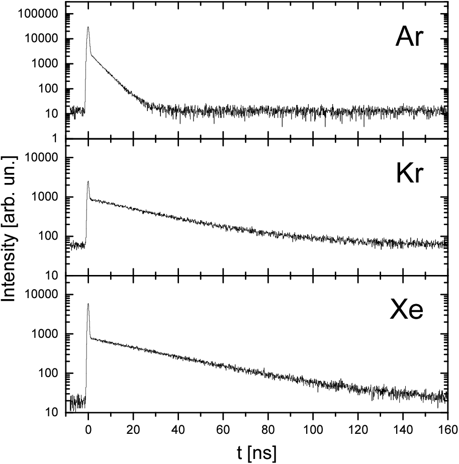

A refined experiment has been performed by Lauer et al. 1999 who used pulsed monochromatized SR and PIFS to measure lifetimes of the subvalence vacancies for Ar, Kr, and Xe. They analyzed the time dependence of the fluorescence intensity after the exciting SR pulse of 0.7 ns FWHM using the single-photon start-stop technique (Schmoranzer and Imschweiler 1984; Lauer et al. 1998b). Typical fluorescence decay curves are depicted in Fig. 36 where the trace of the exciting pulse is observed at . The energy of exciting photons was chosen between the respective threshold and the first satellite with FWHM meV. The measured decay curves were used to derive the lifetimes at each gas pressure and corrected for the collisional de-excitation using Stern-Volmer plots (Schmoranzer and Imschweiler 1984). Results of measurements are listed in the 3rd line of Table 3. One can see excellent agreement between the lifetimes of Lauer et al. 1999 and previous experimental data for Ar and Xe, whereas for Kr a difference by about two orders of magnitude exists.
Lauer et al. 1999 also computed in different approximations according to the schemes (40,41):
| (40) |
where the designations correspond to scheme (23). A calculation taking into account the pathway main (40) only results in too short lifetimes (see line PF in Table 3). Destructive interference between pathways main (40) and sat (41) strongly decreases the transition moment, increasing the lifetimes (see line PF+DPES in Table 3). Both results are in accord with findings of Luyken 1972; Hansen and Persson 1979.
| (41) |
In addition to interactions and effects considered by those authors, Lauer et al. 1999 considered the screening of the Coulomb interaction. Correlations contributing strongly to the main and satellite transitions are shown in schemes (40) and (41). The values near each correlation are the contributions in per cent to the transition amplitude main and sat in schemes (40) and (41), respectively. Corresponding lifetimes computed with taking into account all pathways are listed in Table 3 in line CIPF. One can see that the Coulomb screening significantly improved the agreement between theory and experiment for Xe.
A long-scale calculation of lifetimes for the Ar II main and manyfold satellite levels has been made by Hibbert and Hansen 1987; Hibbert and Hansen 1994 who applied an ab initio CI approximation to this problem. For Xe II, lifetimes of some satellite levels have been computed by Ehresmann et al. 2010.
In conclusion, lifetimes of the subvalence vacancies provide a very sensitive test of many-electron theories because of frequently occurring strong destructive interference. Albeit the physics behind the radiationless decay of the subvalence vacancies seems clear, up to now there are no calculations providing a good agreement between theory and experiment for of all rare gases.
6.2.3 Cross section calculations
When it became clear that the threshold photoionization of the subvalence shells is strongly influenced by intershell correlations, numerous theoretical and experimental investigations of this process appeared (see Section 4.3 and Figs. 19,19) which sometimes gave different results. A precise measurement of the Ar (Sukhorukov et al. 1992; Möbus et al. 1993) revealed a rich resonance structure of near the threshold. The cross sections agreed well with previous data of Houlgate et al. 1976 which fortuitously were located in the peaks of resonances but in average were lower than the computed (see upper left panel of Fig. 34).


A similar situation has been found by Ehresmann et al. 1994 in the case of the Kr (see Fig. 38). One can see that the values of Samson and Gardner 1974 lie on the peaks of resonances revealed in (Ehresmann et al. 1994) and in average are lower than those computed by Schmoranzer et al. 1993. In the high exciting-photon energy region, of Ehresmann et al. 1994 turned out lower than the measurement of Aksela et al. 1987 and the calculation of Tulkki et al. 1992b due to unknown reasons (see Fig. 38).
| Intermediate | Correction | Intermediate | Correction |
| configuration | configuration | ||
| 7.5 | 5.9 | ||
| 6.3 | 5.8 | ||
| 1.0 | 2.5 | ||
| 0.0 | 1.7 | ||
| 0.4 | 0.6 | ||
| 2.7 | 5.5 | ||
| 3.6 | 2.7 | ||
| 0.3 | 0.4 | ||
| 0.4 | 0.5 | ||
| 2.1 | 1.7 | ||
| 0.3 | 0.4 | ||
| other | 2.4 | other | 3.1 |
| Sum | 30.6 | Sum | 27.0 |
a) The values of and are equal to 0.01 Ry and 1.0 Ry, respectively.
b) Summation and integration over the channel AOs in braces were performed.
Sukhorukov et al. 1994b computed the screening of the Coulomb interaction determining the intershell correlations. A typical result of this calculation is listed in Table 4 for Kr (second column). In this column, the partial decreasing coefficients for the matrix element with energies of the continuum electrons Ry and Ry are listed. For other energies, the partial decreasing coefficients are slightly different but the resulting coefficient changes only slightly (Sukhorukov et al. 1994b).
The Coulomb screening for the intershell correlation in Xe had been computed by Lagutin et al. 1996. This result is listed in the fourth column of Table 4. One can see that partial channels connected with electrons having high orbital angular momentum are larger in the case of Xe than in Kr. However, the resulting decreasing coefficient changes only slightly, in contrast to the case shown in Table 2 for the DPES.
Fig. 38 shows that the photoionization cross section of Kr computed with the ‘screened’ intershell interaction (or correlational decrease) fits very well the ‘averaged’ near-threshold cross section. The far region of exhibits also good agreement between the theory of Sukhorukov et al. 1994b and the experiment of Ehresmann et al. 1994 (see Fig. 38). In the region close to the Cooper minimum, the cross section computed within the non-relativistic CIHF approach is too large in comparison with experiment. Good agreement between measured and computed in the whole energy interval has been achieved by Lagutin et al. 1998 after taking into account relativistic effects within the configuration-interaction PF (CIPF) approach (see also Fig. 26 and comments there). The CIPF approach provides also good overall agreement between theoretical and experimental of Xe (see Fig. 26).
6.3 Extended investigations of the resonance structure in PICSs
The doubly excited states have been included in the calculation of the cross sections for excitation of the main and satellite levels of Kr by Lagutin et al. 1994. This calculation allowed to describe qualitatively the rich resonance structure in PICSs of the main line and in some satellite levels of Kr II observed by Schmoranzer et al. 1993 at a resolution (bandwidth of the exiting radiation) of meV. However, the integrated cross sections for the satellite production computed by Lagutin et al. 1994 exceeded the measured ones by a factor of 4.
In order to clarify the mechanisms determining main line and satellite production, a series of combined experimental and theoretical investigations have been performed. Experimentally, the PIFS method at high resolution was used with an extension allowing the simultaneous measurement of both the partial photoionization (PICS) and the photoabsorption (PACS) cross sections. The calculation was carried out applying the CIPF technique.


Lauer et al. 1998a measured and the PACS of Ar at a resolution of meV for exciting-photon energies eV exceeding the threshold eV. Using the same setup, the near-threshold cross sections for the main lines simultaneously with the PACS have been measured by Schmoranzer et al. 2001a at resolutions of meV for Kr and meV for Xe. The results of these measurements are depicted in Fig. 40. One can see that the high resolution allowed to clearly observe the Fano profiles both in the PACS and in the PICS which had not been seen in earlier measurements (cf. PICS of Kr in the middle panel of Fig. 40).
Experimental cross sections of the main line and some of the lowest satellite levels have been measured at a resolution of meV by Ehresmann et al. 2004a in the region of eV. The achieved resolution enabled clearly to observe Rydberg series which were analyzed using the well known formula:
| (42) |
connecting the energy of resonance, , with its principal quantum number , the quantum defect of the -series and the respective threshold energy . Results for two Rydberg series converging to the and thresholds are depicted in Fig. 40 together with positions of resonances computed with equation (42). Extended measurements in a broader exciting-photon energy range ( eV) were presented in (Sukhorukov et al. 2007) together with a refined analysis of the observed Rydberg series, performed on the basis of the CIPFCP calculation. This analysis for the and Rydberg series resulted in quantum defects and , respectively, which is in good agreement with the value of calculated within the CIPFCP approximation for the electron configuration .
Cross sections for the main line of Ar ( eV) and for the three lowest satellite levels , ( eV) have been measured at a resolution of meV by Kammer et al. 2006. The Rydberg series converging to the and thresholds were used by Kammer et al. 2006 for calibration of the exciting-photon energy scale with an estimated accuracy of a few meV.
Measurements of the fluorescence cross sections for the main line and eight satellite lines of Xe have been performed by Ehresmann et al. 2010 and consisted of two experiments. One experiment aimed to get the overview fluorescence cross section in a broad interval ( eV) of the exciting-photon energies at a comparatively low resolution of meV. Another experiment was focused on detailed features in a narrow energy interval ( eV) with extremely high resolution of meV. The cross sections computed by Ehresmann et al. 2010 within the CIPF approach exhibited good agreement with the experimental results, especially in integrated form.
6.3.1 Interaction between resonances through autoionizing continua
The reason for the large difference between computed and measured integrated cross sections for satellite production has been clarified by Demekhin et al. 2005 and Petrov et al. 2005. These authors applied the following scheme to reveal the physical mechanisms determining the main line and satellite production in the photoionization of Kr:
| (43) |
where the designations are the same as in (23): the dashed and double-side arrows denote electric-dipole and Coulomb interaction, respectively; ISCI and FISCI denote the initial and final state configuration interaction, respectively; summation and integration are performed over the channels shown in braces, etc. Besides the correlations indicated in (43), all Coulomb interactions were screened as described in section 6.2. Interaction between the FISCI continuum channels entering the scheme (43) was included via the K-matrix technique.
Scheme (43) describes the following many-electron correlations:
- (i)
-
intrashell correlations are described by pathway and change the transition amplitude describing the photoionization of the shell via accounting for the correlative motion of electrons inside the same shell.
- (ii)
-
intershell correlations change strongly the transition amplitude via the pathway , i.e. photoionization of the shell, via the transition through the shell (so-called ‘borrow-intensity’ mechanism).
- (iii)
-
dipole polarization of electron shells. This correlation is described by the interaction between the configuration and the channel . The influence of such kind of interaction was already discussed for Xe (see scheme (34))
Cross sections for the satellite production borrow intensity mainly from the photoionization via the , and pathways. The influence of the doubly-excited states on the direct main and satellite photoionization is described by the and interactions, respectively, and manifests itself in a strong modulation of the photoionization cross sections.
The calculation performed by Petrov et al. 2005 clarified the many-electron correlations providing the correct strength of the ‘borrow-intensity’ mechanism. It turned out that the integrated intensity of satellites is strongly dependent on two factors: (i) relaxation of the and atomic orbitals and (ii) interaction between resonances through the autoionizing continua. Including these effects substantially decreases the computed fluorescence cross sections. For instance, the relaxation decreases the computed cross sections integrated within the exciting-photon energy region (27.48–28.68 eV) by factors of 1.33, 2.44, and 2.27 for the , , and levels, respectively. Taking into account the interaction between continua results in an additional decrease of the integrated intensity by factors of 3.00, 2.27, and 3.30, respectively. The resulting decreasing factors (4.0, 5.5, and 7.5) provide agreement between computed and measured cross sections within 10 %. Similar results have been obtained by Demekhin et al. 2005 in the energy interval (27.90–29.93 eV).

In detail, the interaction between different resonances including several Rydberg series has been investigated by Sukhorukov et al. 2007 applying (43). In their calculations, the authors removed all resonances from the exciting-photon energy region and included them in the following step-by-step. The results of the calculations in each step are depicted in Fig. 41. In order to monitor the changes in the oscillator strengths, the cross sections f integrated over the interval and having the dimension of are listed in each panel of this figure.
The following approximations in the calculation of the cross sections were used:
- (a)
-
The resonance only was included in the region eV. Fig. 41(a) shows that this broad resonance promotes the intensity from the photoabsorption via the transition providing practically all the intensity in the investigated region and is, therefore, called a promoter. The small intensity at 28.67 eV originates from the resonances which are outside the investigated region before solving the secular equation.
- (b)
-
In addition to the approach (a), the resonances were included. These resonances do not contribute much to the oscillator strength: it is increased by 38%. The resonances shift the promoter and redistribute intensity within the investigated region.
- (c)
-
In addition to the approach (b), the Rydberg series was included. The interaction between the Rydberg series and the promoter results in quite a regular structure. The integrated cross section remains practically unchanged. On an enlarged scale (not shown in the figure), one can see the well known ‘sign-reversal’ behaviour of the parameter (Connerade and Lane 1988) around the resonance with an energy of 28.532 eV. This resonance which can be considered as an intruder resonance or as a ‘remaining promoter’ increases the amount of resonances connected with the Rydberg states by one.
- (d)
-
In addition to the approach (b), the Rydberg series was included. The ‘sign-reversal’ behaviour of the parameter can be seen around the intruder resonance with the energy of 28.542 eV (between the Rydberg resonances and ) which can be interpreted as the ‘remaining promoter’.
- (e)
-
In order to illustrate the ‘own’ intensity of the and Rydberg series, they were included in the calculation excluding the promoter. Fig. 41(e) illustrates that (i) the ‘own’ intensity is 7 times smaller than the promoted intensity; (ii) the major part of the ‘own’ intensity stems from the Rydberg series, whereas the Rydberg series is not seen within the ordinate scale of Fig. 41(e).
- (f)
-
In addition to (b), the ‘low-number’ Rydberg series were included. This approach shows the role of the ‘low-number’ () Rydberg states stemming from the and levels in the formation of the investigated structure. These states increase the oscillator strength by 8% and yield some features around 28.44 eV, 28.50 eV, 28.59 eV, and 28.65 eV. In the experimental spectrum depicted in panel (j), these features are clearly seen as a bell-shaped ‘background’ below the resolved resonances, e.g., at 28.61 eV and 28.65 eV.
- (g)
-
In addition to (f), the Rydberg series were included. Including the series results in two small resonances at 28.452 eV and 28.615 eV and the pronounced profiles of the resonances stemming from the doubly-excited states. In order to see whether it is possible to observe these features experimentally, the calculation (h) was performed.
- (h)
-
In this approach, the Rydberg series were excluded from the most precise approach (i). The features connected with the and doubly-excited states are difficult to identify in the experimental spectrum (j), whereas the pronounced profile stemming from the doubly-excited states can be seen there.
In conclusion, the combined experimental and theoretical investigations shed light on the main mechanisms determining the photoionization of the rare gas atoms in the vicinity of the subvalence threshold. A correct interpretation of the observed photoionization cross section requires to take into account intershell and intrashell correlations, dipole polarization of the shell by the vacancy, Coulomb screening, relaxation of electron shells upon the vacancy, and interchannel interaction. In addition, near-threshold photoionization of the main and satellite levels requires to take into account numerous doubly excited states. The inclusion all of these interactions in the calculation allows to describe many of the observed spectral features, including integrated cross sections and line shapes in many cases.
6.3.2 Photoionization of rare-gas atoms between the and thresholds
The amount of pronounced resonances observed in the cross sections of between the valence and subvalence thresholds is much smaller than that observed in the main and satellite photoionization cross sections described in the previous section. Autoionizing resonances lying between the and thresholds in represent a very important phenomenon allowing to precisely study different types of many-electron correlations. The interaction between and continua results in well known interference profiles described by Fano 1961 (see equation (31)). The parameters of those autoionizing resonances are very sensitive to the approximations used in calculations and allow to draw conclusions about the adequacy of the approach.
Autoionizing resonances in the total photoionization cross sections of He, Ne, and Ar have ‘Beutler-Fano’ shape, as it has been observed by Madden and Codling 1963 who used synchrotron radiation as excitation source and presented a densitometer trace for the He photoionization. Later on, the observation of the resonances has been revisited several times. Samson 1963 presented photoionization cross sections measured for Ar and Kr using a high-voltage repetitive spark discharge in Ar as excitation source.
Refined measurements of the resonances have been performed by Codling et al. 1967 for Ne, by Madden et al. 1969 for Ar (see Fig. 12), and by Ederer 1971; Codling and Madden 1972 for Kr and Xe. The measurements of Codling and Madden contain the above--threshold region, too (see Fig. 12). The ‘window’ type of the main autoionizing resonances observed in Ar, Kr, and Xe indicate that the imaginary part prevails in the transition amplitude.
The first calculation of the resonances line shapes has been performed by Kelly and Simons 1973 for Ar within the many-body perturbation theory. In this calculation, they took into account the intrashell correlations and neglected the DPES. Nevertheless, they obtained a fairly good agreement between the calculated and the measured total PICS of Madden et al. 1969. It can be assumed that the used approximation would result in a poor description of the PICS above the Cooper minimum (see Fig. 17) and of the correlation satellites. Thus, the calculation of Kelly and Simons 1973 can serve as an example that an approximate calculation can give a good description of a part of the experiment only.
Burke and Taylor 1975 applied the R-matrix theory to describe the autoionizing resonances and their parameters , , and entering equation (31). They found that taking into account many-electron correlations substantially changes the resonance parameters, even changing the sign of the quality parameter . Good agreement between measured and computed values of resonance parameters has been obtained. A large number of many-electron correlations included in the calculation took into account to a large extent the DPES and the Coulomb screening. However, a detailed analysis of the influence of each correlation on the computed quantities is absent in this paper. Also Burke and Taylor 1975 did not discuss the shift of the computed cross section in comparison with the measured one (see Fig. 19). It can possibly be connected with the use of a semiempirical core polarization potential in the AO calculation of these authors or with the used approximation accounting for DPES.
Wijesundera and Kelly 1989 applied many-body perturbation theory to compute the influence of single-electron excitations () and of doubly excited states on the photoionization of the and shells and of the satellites. They were the first who showed the importance of including doubly excited states in the calculation of the near--threshold photoionization of Ar. However, the computed line shapes of the resonances in the photoionization did not reproduce the experimental data well. Supposedly, this is due to the fact that the authors did not fully take into account Coulomb screening (at least, the configuration , which largely determines the Coulomb screening (see, e.g., Table 2), is absent in the list of electron configurations included in the calculation).
Photoelectron spectroscopy provided a new possibility to measure the shape of the autoionizing resonances in the partial PICS specified by the total angular momenta of the core vacancy. Samson and Cairns 1968 were the first who presented experimental partial PICS for Ar, Kr, and Xe. The resolution of the photoelectron spectrometer in this first experiment was rather low but, nevertheless, allowed the authors to observe that some resonances have a ‘peak’ shape in the cross section and a ‘window’ shape in the one (or vice versa). Thus, these resonances, being strong in and , cancel each other and result in only a weak resonance in the total photoionization cross section. Later on, autoionizing resonances of such kind have been called ‘mirroring’ resonances.
The angular distributions of photoelectrons in the region of the resonance in Ar and of the resonance in Xe have been measured by Codling et al. 1980. Ederer et al. 1982 measured the shape of the resonances in Kr and Xe and determined partial cross sections at a resolution of meV. The angular distribution parameter of the photoelectrons , specified by the total angular momentum of the vacancy, has also been measured in this work. Analyzing the experimental data, Ederer et al. 1982 pointed out the necessity to take into account doubly excited resonances stemming from the correlation satellite levels.
Wills et al. 1989 used photoelectron spectroscopy to measure the autoionizing resonances in an extended exciting-photon energy range at a resolution of meV. They presented results for Ar (Wills et al. 1989), Xe Wills et al. 1990a, and Ne Wills et al. 1990b, which for Xe were specified by the total angular momentum of the vacancy.
Flemming et al. 1991 measured cross sections and photoelectron angular distribution parameters for the energy regions 20.6—21.5 eV in Xe and 24.6—25.3 eV in Kr at a high resolution of meV. They clearly observed resonances connected with the doubly excited states for both atoms. Flemming et al. 1991 analyzed the measured line shapes of the resonances in terms of the Shore 1967 parameters.
The relationship between the Fano and Cooper 1965 and Shore 1967 parameters was investigated in great detail by Sorensen et al. 1994. They also performed a calculation of the line shapes within the MMCDF approach of Tulkki et al. 1992a neglecting, however, the DPES and Coulomb screening.
An extended calculation of the autoionizing resonances has been performed for Ar by Lagutin et al. 1999, for Kr by Demekhin et al. 2005, and for Xe by Sukhorukov et al. 2010 within the CIPFCP approximation. They took into account a multitude of many-electron correlations such as: (i) intrashell and intershell correlations; (ii) DPES; (iii) Coulomb screening; (iv) interaction between resonances stemming from the main level and from the satellite levels (direct and via continua); (v) interchannel interactions. For Kr and Xe, the specific cross sections and the photoelectron angular distribution parameters were also computed.

The partial and the total photoionization cross sections computed by Demekhin et al. 2005 for Kr () and by Sukhorukov et al. 2010 for Xe () are compared with the respective measurements of Flemming et al. 1991 in Fig. 42 for the energy region around the first resonances. In both cases, the computed cross sections are in good agreement with the measured ones.
The identification of resonances is listed in Table 5. In the first two columns, the numbering of resonances corresponding to Fig. 42 and the computed resonance energies, respectively, are listed. The 3rd column shows the largest coefficient (in per cent) in the linear combination of the doubly excited states (27). The 4th column shows the largest coefficient (in per cent) in the core wave function (16) and the quantum numbers of the core. It is possible to indicate the genealogy of the main and satellite levels in the majority of cases, especially in Kr. In case of the resonances, the percentage of the dominating component in the doubly excited state hardly exceeds % due to the strong interaction between the doubly excited states stemming from the main and satellite levels. This makes the identification of the autoionizing resonances in Kr and Xe to a large extent conventional.
| Kr from (Demekhin et al. 2005) | Xe from (Sukhorukov et al. 2010) | |||||||||
|---|---|---|---|---|---|---|---|---|---|---|
| no | [eV] | % | Doubly excited state b) | no | [eV] | % | Doubly excited state b) | |||
| a) | Ion state | a) | Ion state | |||||||
| 1 | 24.732 | 29 | 67% (3P)5s 4P3/2 | 5p3/2 | 1 | 20.319 | 31 | 87% (3P)6s 4P5/2 | 6p3/2 | |
| 2 | 24.811 | 52 | 64% 4s 2S1/2 | 5p1/2 | 2 | 20.692 | 33 | 47% (3P)6s 2P3/2 | 6p1/2 | |
| 3 | 24.929 | 17 | 96% (3P)5s 4P5/2 | 5p3/2 | 3 | 20.819 | 75 | 55% (5s) 2S1/2 | 6p1/2 | |
| 4 | 24.960 | 36 | 67% (3P)5s 2P3/2 | 5p1/2 | 4 | 20.992 | 65 | 55% (5s) 2S1/2 | 6p3/2 | |
| 5 | 25.008 | 23 | 64% 4s 2S1/2 | 5p3/2 | 5 | 21.032 | 33 | 47% (3P)6s 2P3/2 | 6p3/2 | |
| 6 | 25.185 | 24 | 93% (3P)5s 4P1/2 | 5p3/2 | 6 | 21.036 | 42 | 60% (3P)5d 4D1/2 | 6p1/2 | |
| 7 | 25.400 | 11 | 93% (3P)5s 4P1/2 | 5p1/2 | 7 | 21.211 | 24 | 69% (3P)6s 4P1/2 | 6p1/2 | |
| 8 | 25.477 | 30 | 67% (3P)5s 2P3/2 | 5p3/2 | 8 | 21.277 | 28 | 80% (3P)5d 4D5/2 | 6p3/2 | |
| 9 | 21.336 | 58 | 56% (3P)6s 4P3/2 | 6p1/2 | ||||||
| 10 | 21.364 | 31 | 60% (3P)5d 4D3/2 | 6p3/2 | ||||||
| 11 | 21.439 | 52 | 60% (3P)5d 4D1/2 | 6p3/2 | ||||||
a) The percentage of the largest component in the doubly excited state.
b) Before the quantum numbers of the ion state, the percentage of its largest component is shown.
Sukhorukov et al. 2010 studied the formation of a resonant structure in the Xe photoionization. For this purpose, they performed two model calculations. In the first one, the Rydberg series was taken into account only, whereas the second one included the Rydberg series converging to the satellite thresholds only. The results of this study are depicted in Fig. 44b and Fig. 44c, respectively. Fig. 44a shows the result of the calculation where all Rydberg series are taken into account.


Fig. 44b illustrates that taking into account the Rydberg series forms the most prominent details in the total cross section, with the most intense components belonging to the series. Rydberg series originating from the satellite ionic states result in relatively small resonances (see Fig. 44c). Taking into account the interaction between the ‘main’ and ‘satellite’ Rydberg series leads to their strong mixing, which manifests itself in a change of the energies and intensities of resonances, and results in a good agreement between theory and experiment (see the right part of Fig. 42).
To verify the accuracy of the calculated wave functions Demekhin et al. 2005 and Sukhorukov et al. 2010 computed the photoelectron angular distribution parameters for Kr and for Xe, respectively. For Xe, the computed is compared with the measured one in Fig 44. The good agreement between theory and experiment demonstrates the adequacy of the CIPFCP approach for describing the atomic photoionization.
6.3.3 Isoelectronic sequences
In the previous sections, it was illustrated how changing intraatomic interactions in the calculation of photoionization cross sections clarifies the major correlative effects. An interesting series of papers has been published by van Kampen et al. 1997, Neogi et al. 2003, and Yeates et al. 2004 who found a way to change the relationship between intraatomic interactions experimentally. To achieve this goal, they investigated the K+ and Ca2+ ions, isoelectronic to Ar (van Kampen et al. 1997), and the Rb+, Sr2+ (Neogi et al. 2003), and Y3+ (Yeates et al. 2004) ions, isoelectronic to Kr. To measure the photoabsorption of these ions, the Dual Laser Plasma (DLP) technique was used.
The DLP technique uses two plasmas created by lasers. One laser operated with pulses of J in 10 ns and produced the plasma column consisting of the ions of interest (the sample) at about 15 eV ( K). The temperature of the expanding plasma decreases with time, lowering the dominant ion stage. The second laser operating in a similar regime produced the second plasma column serving as a source of the VUV exciting photons. Setting a suitable time delay between the operation of the sample source and of the source of the exciting photons, one can investigate the photoabsorption of the selected ions using the spectrometer. The energy resolution in the PACS measurements varies from meV at eV to meV at eV. Here we gave the salient details of the DLP technique only, while its full description can be found in the exhaustive reviews of Costello et al. 1991 and Kennedy et al. 1994; Kennedy et al. 2004.
The investigation of the photoabsorption of the Ar-like ions Ar–K+–Ca2+ by van Kampen et al. 1997 revealed dramatic changes in the shape of the resonances. The parameter of the first resonance in K+, , changed the sign with respect to of Ar (Sorensen et al. 1994). In Ca2+, this resonance ‘lost’ oscillator strength and became less intense than the resonances with , having a peak shape. The calculation performed by van Kampen et al. 1997 explained this behaviour of the resonance shape by the impact of the many-electron correlations, emphasizing the large role of ‘double-electron correlations’ which in the present review are called DPES correlations.
A detailed calculation of the photoabsorption of the Ar-like ions has been performed by Lagutin et al. 1999 within the CIPFCP approximation. These authors illustrated that the strong changes of the shape of the resonances are determined by the complex interrelation between the direct and intershell transition amplitudes including their real and imaginary parts.
A similar behaviour of the line shapes of the resonances in the Kr-like ions Kr–Rb+–Sr2+–Y3+ has been observed by Neogi et al. 2003 (for Rb+, Sr2+) and Yeates et al. 2004 (for Y3+). The results of their observation by the DLP technique are depicted in Fig. 45 together with the PICS of Kr (Codling and Madden 1972). One can recognize several salient features in the behaviour of the resonance line shapes: (i) the parameter varies strongly in the sequence Kr–Rb+–Sr2+–Y3+, being small in Kr () and large in Y3+ (); (ii) in Sr2+, the and resonances exhibit too small oscillator strengths in comparison with the one, and (iii) parameters strongly change along the series.

The calculations of Neogi et al. 2003 and Yeates et al. 2004 showed that the doubly excited states in the ions have larger energy than the first autoionizing resonance, in contrast to Kr discussed above where they strongly overlap with the promoter. In Rb+–Sr2+–Y3+, the doubly excited states result in the rich structure of the second and higher resonances. Therefore, in Fig. 47, we show results from (Yeates et al. 2004) for the first resonance only.


In Fig. 47, the partial and total transition amplitudes are depicted for Rb+–Sr2+–Y3+. For the discrete states, the amplitudes are presented according to (Cooper 1962) as areas proportional to the respective oscillator strengths. From this figure, one can recognize that the intershell correlations result in large real (Corr Re) and imaginary (Corr ImCIPF Im) parts of the partial transition amplitude which are comparable to the direct PF amplitude. The interrelation between all these amplitudes explains all the peculiarities in the behaviour of the autoionizing resonances described above. Indeed, (i) Y3+ has a very small imaginary part of the transition amplitude in comparison with Rb+–Sr2+ which explains the peak shape of the observed resonances (see equation (30) for ); (ii) in Sr2+, the PICS have a minimum in the vicinity of the and resonances which explains their anomalously small oscillator strength; (iii) in Sr2+, the ratio of the imaginary and real parts of the transition amplitude varies strongly along the series which explains the respective behaviour of the parameter.
Fig. 47, where the computed PICS are compared with the measured ones, illustrates how the mirroring behavior of the cross sections and at the resonance explains its absence in the total cross section in Rb+–Sr2+. In Y3+ the component of the first autoionizing resonance can clearly be seen in the total cross section.
In conclusion, the investigation of the isoelectronic sequences allows one to judge about the interrelation between the single-electron and many-electron processes in a wide range of the intraatomic interactions. This information is extremely useful for the creation and development of the ab initio methods for atomic structure calculations.
7 Alignment and orientation of ionic states
When polarized synchrotron radiation excites the atom, the magnetic sublevels are populated non-statistically. For instance, linearly polarized exciting radiation populates the sublevel , whereas the population of the sublevels equals zero (thus, the exited state is fully aligned). Circularly polarized light produces fully oriented states, e.g. right-hand polarized photons excite the sublevel only (see Fig. 48).
During the decay of the excited state, the alignment or orientation is transferred to the decay fragments and results in their anisotropic distribution and polarization. In Fig. 48, the orientation transfer computed for the process is schematically visualized. The non-statistical population of the magnetic sublevels is clearly seen. Thus, studying the angular distribution or polarization of the decay fragments allows to get information about the spectral distribution of the angular momenta of the, e.g. ionic states. This information provides an excellent test of the theoretical models for interpreting experimental data and is useful in the interpretation and disentanglement of the complex structure of the aforementioned core-excited spectra.

In the present chapter, we intend to present the basic results obtained in the polarization experiments by PIFS. Therefore, for the detailed theoretical description of the photofragmentation, alignment, and orientation, we refer the reader to the reviews of Greene and Zare 1982, Schmidt 1992, Kabachnik et al. 2007, and to the book of Balashov et al. 2000 where the details and references to numerous original investigations can be found.
Mehlhorn 1968 stressed that colliding particles will align atoms with respect to the direction of the exciting beam and, therefore, X-ray radiation and Auger electrons should have a nonisotropic angular distribution. Studying that angular distribution has been proposed in order to determine the relative partial photoionization cross sections (Flügge et al. 1972). The basic relations describing the alignment of ions in the ionization process and the following angular distribution of the decay fragments have been obtained by Eichler and Fritsch 1976 and Berezhko and Kabachnik 1977. For example, the angular distribution of the Auger electrons ejected from an atom by linearly polarized photons with energy can be represented by the differential cross section as:
| (44) |
where is the Legendre polynomial, is the angle between the polarization vector of the exciting radiation and the direction of the ejected Auger electron, and is the quantity called photoelectron angular distribution (PAD) parameter. Berezhko and Kabachnik 1977 also calculated the alignment of ions and PAD parameters for some selected cases within the HS approach. In the following, a considerable amount of investigations were focused on the alignment transfer during the resonant Auger (RA) effect after excitation of a deep core electron to the first Rydberg state, e.g. in Kr or in Xe, because these processes look comparatively simple.
7.1 Resonant Auger (RA) effect
The decay of the resonantly excited Kr∗ and Xe∗ states has been observed for the first time by Eberhardt et al. 1978 at a resolution of 0.3 eV and initiated numerous investigations. Measurements of the RA effect were used to investigate post collision interaction (Schmidt et al. 1981; Southworth et al. 1983), the alignment of the Xe+ ions and angular distribution of the Auger electrons (Southworth et al. 1983), and many-electron correlations like DPES (Aksela et al. 1986), etc. (see, e.g., the review Armen et al. 2000 and references therein).
The first measurements of the RA effect and related phenomena were performed at rather low resolution of eV. Better resolution of 150 meV was used by Carlson et al. 1988; Carlson et al. 1989 who measured the Auger electron angular distribution parameters in the resonantly excited Ar∗ (), Kr∗ (), and Xe∗ (). Earlier theoretical treatments of the RA effect were based on the stepwise (or two-step (2ST)) model which implies that the interference between the resonant and direct ionization channels as well as between different resonant channels is ignored. This model was used by Kabachnik et al. 1991 and by Hergenhahn et al. 1991 to compute the spin polarization and the angular distribution of the Auger electrons in the RA decay of Ar, Kr, and Xe. The authors used in the calculation the core AOs obtained by applying the DF package of Grant et al. 1980 and the continuum AOs computed within the relativistic local density approach.
Considerable progress in the investigation of the RA effect has been achieved by experiments in the Raman regime of the excitation of atoms. In this regime, the experimental resolution is smaller than the natural width of the intermediate resonance (Brown et al. 1980; Kivimäki et al. 1993), which makes it possible to observe the majority of the final ionic states. The influence of many-electron correlations in both the initial and final states of the RA effect on the angular distribution of the Auger electrons has been investigated by Tulkki et al. 1994 within the MMCDF approach (see section 3.2).
The Raman regime was utilized to observe many new experimental features in the ordinary RA spectra of Kr (Aksela et al. 1996a; Jauhiainen et al. 1996) and to measure in the RA spectra of Kr (Aksela et al. 1996c) and Xe (Aksela et al. 1996b). In order to interpret the experiments, these authors performed calculations using the theoretical technique of Tulkki et al. 1994.
Ehresmann et al. 1998 applied the PIFS technique to measure the alignment of the Xe II ions obtained in the following process:
| (45) |
where the designations are the same as in (23): the dashed and double-side arrows denote electric-dipole and Coulomb interaction, respectively; [0] denotes the ground state of the atom and the internal quantum numbers of atomic and ionic states are self-explanatory. All transitions in scheme (45) are initiated by the exciting photon , while the fluorescence photon is registered. The measurements for Xe were revisited at higher accuracy by Lagutin et al. 2000 and a similar experiment for Kr was performed by Zimmermann et al. 2000.
Different experimental setups have been applied by those authors: to measure the alignment of the Xe+ states, Lagutin et al. 2000 applied the technique of the ‘crossed undulators’ (see Fig. 8 and comments to it), while for the Kr+ states, Zimmermann et al. 2000 used the ‘Wollaston prism’ setup (see Fig. 6). In order to compute the alignment parameters , Lagutin et al. 2000 and Zimmermann et al. 2000 used the 2ST model and the CIPF approximation according to the following formula (see, e.g. (Schartner et al. 2007)):
| (46) |
where the kinematics coefficients can be found in (Lagutin et al. 2000; Zimmermann et al. 2000; Lagutin et al. 2003a). The reduced partial cross sections
| (47) |
were computed using the cross sections and determined by equation (24). The absolute values of the calculated alignment parameter appeared to be systematically larger than the measured ones. This was partly attributed to the disalignment of ions due to cascade transitions, which have an estimated probability of 8.5% in comparison with the main process (45) (Lagutin et al. 2000). The strongest disalignment channel contributes 75% of that total probability. Additional disalignment of the ionic states is connected with the hyperfine interactions (Meyer et al. 2001). The PAD parameters for the RA decay in Kr and Xe were computed in (Zimmermann et al. 2000; Lagutin et al. 2000) also.
7.1.1 Beyond the two-step model
All the above papers used for the interpretation of the experimental data the 2ST model, treating the RA decay as two independent steps. The first step leads to the excitation of the intermediate atomic resonances which decay during the second one. The limitation of the 2ST model has been pointed out by Camilloni et al. 1996; Kukk et al. 1997; Saito et al. 2000; De Fanis et al. 2002. In these papers, the parameters for individual RA lines in the resonance excitation of Ar (Camilloni et al. 1996), Kr (Kukk et al. 1997) and Ne (Saito et al. 2000; De Fanis et al. 2002) were found to depend on the excitation energy. The 2ST model cannot explain these observations.
Lagutin et al. 2003a; Lagutin et al. 2003b performed a combined theoretical and experimental investigation of the RA effect in Kr. These authors measured the energy dependence of the alignment of some selected ionic states being populated via the RA decay of the resonances using the crossed undulators PIFS technique (see Fig. 8). These resonances, having a natural width of 83 meV (King et al. 1977; Sairanen et al. 1996), were scanned within the Raman regime at a resolution of 10 meV by steps of 5 meV.

In order to compute the alignment parameters , Lagutin et al. 2003a; Lagutin et al. 2003b applied the CIPF approach (see section 3.3) taking into account interference between the resonant (R) and direct ionization (dir) channels and between different resonant channels (see scheme (45)). In this approximation, the transition amplitudes determining the dynamics of all processes are given by:
| (48) |
where and are the Coulomb and electric dipole operators, respectively; is the total width of the resonance. The first term entering equation (48) describes the direct photoionization and the sum over in the second term includes all resonance channels. In Kr, four resonances lie in the range of interest at the computed energies (coinciding with the measured ones within several meV) (91.200 eV), (92.424 eV), (92.454 eV), and (92.565 eV). Resonances and are practically pure and basis states, respectively, whereas resonances and are perceptible mixtures of the and basis states. The oscillator strength for the resonance is 1/80 of the resonance only, so that it was excluded from consideration.
The results of the calculation for two selected ionic states excited at energies close to the and resonances are depicted in Fig. 49 together with the experimental data. In this figure, the results of three calculations are presented: (i) the 2ST results are shown as horizontal bars; (ii) the dashed curve shows the result without taking into account direct ionization (dir) (for the level, the (dir) pathway is forbidden by a selection rule); (iii) solid lines represent the results of the complete calculation. One can recognize the following:
- (a)
-
the interference between the (R2) and (R4) pathways only results in substantial changes of computed within the 2ST model (see the results at the resonance);
- (b)
-
the interference between the (R) and (dir) pathways noticeably changes the computed ;
- (c)
-
the computed energy dependences are in good agreement with the measured ones, resulting, however, in a little larger values. This discrepancy can be attributed to the disalignment of ionic states which was not taken into account in the calculations of Lagutin et al. 2003a; Lagutin et al. 2003b.
The coherent treatment of the partial transition amplitudes resulted in better agreement between computed and measured alignment parameters for the majority of the ionic states in Kr (Lagutin et al. 2003a). The remaining differences between theory and experiment have been discussed by Lagutin et al. 2011 who included in the calculation cascade transitions and four-fold excitations in the vicinity of the resonances.
The Raman regime was also used by Sankari et al. 2007 in a combined investigation of the RA decay of the resonances of Kr∗. These authors used photoelectron spectroscopy at a resolution of 25 meV to cover the exciting-energy range from 92.12 to 92.87 eV by 10 meV steps to measure the population of the ionic states and the respective PAD parameter . In order to compute the measured quantities, the authors applied the RATIP suite (see section 3.2). The population of the ionic states has also been investigated by Sankari et al. 2008 using the PIFS technique. The calculation performed by these authors includes also cascades. In both papers, the importance of taking into account the (R) and (dir) pathways coherently has been confirmed.
7.2 Partial wave analysis
In the photoionization of the closed-shell Rg, the cross section for the population of the ionic state is determined by the three partial waves (Klar 1980; Greene and Zare 1982) (see equation (24) for details):
| (49) |
According to equation (49) one can define the dimensionless reduced partial wave cross sections
| (50) |
interconnected by the normalization condition:
| (51) |
The three reduced partial cross sections determine also the alignment and orientation parameters as (Klar 1980; Greene and Zare 1982):
| (52) |
| (53) |
with the kinematics coefficients tabulated, e.g., in (Lagutin et al. 2003a). Solving equations (51) to (53) we get
| (54) |
where the kinematics coefficients and are tabulated, e.g. in (Schartner et al. 2005), and ( is the total angular momentum of ion plus photoelectron, see Schartner et al. 2007). Thus, the two observables and provide sufficient information to derive the reduced partial wave cross sections .
Schmoranzer et al. 1997a, Mentzel et al. 1998, and Yenen et al. 1997 obtained the alignment parameters using different setups of the PIFS technique: Schmoranzer et al. 1997a and Mentzel et al. 1998 applied the ‘crossed undulator’ setup (see Fig. 8) while Yenen et al. 1997 analyzed the polarization of fluorescence. Schmoranzer et al. 1997a measured for the even states of Kr II at a resolution of meV. Yenen et al. 1997 obtained the polarization of the odd state of Ar II at a resolution of meV. Mentzel et al. 1998 reported measured for seven odd states of Ar II at a resolution of meV.

Typical results of the measurements of Mentzel et al. 1998 are shown in Fig. 50 for two selected levels. Schmoranzer et al. 1997a and Mentzel et al. 1998 used the intensities obtained for the undulators operating in vertical () and horizontal () modes, respectively, to derive the fluorescence angular distribution parameter via
| (55) |
kinematically connected with (Berezhko and Kabachnik 1977) by
| (56) |
where is the total angular momentum of the final state of the fluorescence process (numerical coefficients can be found, e.g., in (Lagutin et al. 2003a)). We note that the alignment can also be determined when the atom is ionized by circularly polarized radiation. In this case the quantization axis coincides with the direction of the exciting radiation (as, e.g., in (McLaughlin et al. 2002)) referred to as - axis and , respectively. This alignment is connected with by (Schmidt 1992).
An advanced PIFS setup using a Wollaston prism (see Fig. 6) has been applied by Zimmermann et al. 2004 to measure the alignment parameters of the odd states of Ne II in the exciting-photon energy range of at a resolution of 18 meV. In addition, these authors obtained PICS for the population of the even and states at the high resolution of 4.5 meV.
The orientation parameter for the odd state of Ar II has been measured by McLaughlin et al. 2002 using circularly polarized exciting photons obtained by application of a four-reflector quarter-wave retarder to the initial linearly polarized synchrotron radiation. Using the technique described above (Yenen et al. 1997), the authors measured also . Having and equations similar to (52), (53), McLaughlin et al. 2002 derived the reduced partial wave cross sections in the exciting-photon energy range .
Calculations of the energy dependence of the alignment and orientation parameters are rather scarce. van der Hart and Greene 1999 computed and for the state of Ar II using the R-matrix technique described earlier (van der Hart and Greene 1998). Later on, the same technique has been applied for the calculation of the orientation parameter and of for some selected even states (van der Hart and Greene 2002). The calculations of these authors qualitatively reproduced many of the experimentally observed features. However, some of the computed features deviated (sometimes up to 0.1 eV) from the measured ones. Supposedly, this disagreement can be connected with neglecting Coulomb screening (see section 6.2) in the calculations.
The absolute partial PICSs for the even states of Kr II were calculated by Schmoranzer et al. 1997a, allowing these authors to compute the respective fluorescence angular distribution parameters, too. More precise calculations of these parameters have been performed by Demekhin et al. 2005 within the CIPF approximation. In this paper, PICSs and the alignment parameters for the and states were also computed and measured. The comparison of theory and experiment led to the conclusion that core rearrangement and coherently taking into account the autoionizing resonances and the autoionization continua strongly influence the computed quantities.
Schill et al. 2003 and O’Keeffe et al. 2003; O’Keeffe et al. 2004 performed a partial wave analysis (PWA) of the RA decay of resonantly excited Kr and Xe using the ‘sitting-on-resonance’ regime. Schill et al. 2003 used the setup shown in Fig. 6 to measure alignment and orientation of the Kr II state after the decay of the resonance. Using equations (51) to (53) results in the ratios which coincide with the predicted ones by Zimmermann et al. 2000 within the error bars.


O’Keeffe et al. 2003 measured the orientation of five selected Xe II states after the decay of the resonance and used the alignment parameters from Meyer et al. 2001 to perform the PWA of this decay. A combined theoretical and experimental investigation of the RA decay of the resonance with following population of the Xe II states has been performed by O’Keeffe et al. 2004. These authors found a good overall agreement between the measured and computed PWA including also the calculation of Lagutin et al. 2000.
The Raman regime for the PWA was used by Schartner et al. 2005; Schartner et al. 2007 who populated the Kr II states via the to resonances ( meV, see section 7.1.1) at a resolution of meV. The alignment parameters and the orientation parameters were measured for the and states in (Schartner et al. 2005) and for the state in (Schartner et al. 2007). These measurements enabled the authors to determine the reduced partial wave cross sections in the exciting-photon energy range of . The and results for the state are depicted in Fig. 52. In this figure, where the results of the calculation from Schartner et al. 2007 are also shown, one can see good overall agreement between theory and experiment. The comparison between calculations performed without and with taking into account the non-resonant channel emphasizes the importance of the latter. Fig. 52, where the results of the experimental and theoretical PWA are depicted on an enlarged scale, shows the interrelation between partial waves passing through resonances.


Concluding this section we mention an experimental technique which differs from PIFS and allows to measure the partial photoionization cross sections quantified by the total angular momentum of the final state. Aloïse et al. 2005 reported the experimental ‘two-colour’ setup consisting of two radiation sources: the synchrotron radiation (SR) was used to prepare the intermediate resonant state while a tunable dye laser was used for the subsequent photoionization from this state. The authors used an experimental scheme with two collinearly counterpropagating exciting-photon beams of variable linear and circular polarization. The photoion current was measured depending on the varied mutual polarization between SR and laser radiation. Using linearly and circularly polarized light makes it possible to derive linearly independent equations connecting the photoion current measured at different polarization as input data and the partial photoionization cross sections as unknowns. Solving these equations results in partial PICS.
Aloïse et al. 2005 applied the two-colour technique to study several processes among which was the following ( coupling is used for the notation of the atomic states):
| (57) |
where the notations of arrows are the same as in (23). Two of the ion yields (for the different mutual orientations of the linearly polarized SR and laser) are depicted in the upper panel of Fig. 54 as an example. In the panels below, the partial cross sections derived from the measured ion yields are shown. The positions of the resonances are marked on top. It is clear that the resonances affect those cross sections only that have the same value of because the Coulomb interaction is a scalar. Measured partial and total cross sections are compared with the ones calculated by Petrov et al. 2006 within the CIPFCP approximation in Fig. 54. Good agreement between all computed and measured cross sections allows to state the adequacy of both the theoretical and experimental techniques.
8 Summary and perspectives
In summary, we reviewed the work on the dynamics of photon-induced atomic processes over the past half century showing that many of them are largely determined by many-electron correlations. We pursued chronologically how our understanding of the photoionization process developed, when the measurements initiated the development of the theory and then the development of the theory required to reconsider the results of the experiments and to carry out refined measurements. One of the examples is the photoionization of the subvalence shells of rare-gas atoms. In this case, based on the calculations, the presence of a minimum in the photoionization cross section was predicted which visually looks like a Cooper minimum but actually has a substantially different nature. This many-electron nature should also lead to an anomalous angular distribution of photoelectrons. Subsequently, the predictions were confirmed qualitatively by experiments, but the experiments revealed also a significant discrepancy between measured and computed cross sections. This, in turn, stimulated the development of the theory and new methods for calculating atomic structures.
We have paid special attention to cases where the PIFS results significantly improved the understanding of atomic processes. For example, PIFS made it possible to reliably register a resonant structure in the near-threshold photoionization of the rare-gas atoms, which in turn constituted a challenge for creating new precise methods for the atomic structure calculations. One of such methods was based on the Pauli-Fock (PF) approximation, which allows one to take into account relativistic effects saving the one-component structure of AOs on the one hand, and ensures high accuracy of calculation on the other hand. The PF AOs were used to take into account all electron configurations differing from the state of interest by single- and double-excitations. Strongly interacting configurations were taken into account via the solution of the secular equation while the other configurations were taken into account by computing the corrections to the matrix elements of that equation (usually reducing them and, therefore, called the Coulomb screening). Some selected excitations were included in the calculation by means of a non-empirical core polarization (CP) potential and following recalculation of the set of the PF AOs, thus generating a new complete set of the PFCP AOs. Using the CIPFCP (configuration interaction Pauli-Fock with core polarization) technique made it possible to understand the origin of most of the features observed by PIFS. In turn, the development of the CIPFCP approach initiated the investigation of new interference phenomena by the PIFS method. In particular, it has been shown that the alignment of atoms in a resonant Auger decay is significantly affected by interference between different photoionization pathways that can be observed experimentally.
The PIFS method allowed to reliably determine the lifetime of rare-gas atoms with a subvalence vacancy, which is anomalously large because of the destructive interference between the main and satellite processes. The measured lifetimes agree reasonably with the computed ones which confirms the adequacy of the considered mechanism. In photoelectron spectra, such an interference causes a strong dependence of the spectra on the exciting-photon energy in the threshold range: some well-resolved lines change their relative intensity by more than an order of magnitude.
In a further development of PIFS, methods for measuring the alignment and orientation of atoms and ions excited by polarized radiation and for performing partial wave analysis have been created. The use of partial waves in turn helps to improve the methods of the atomic structure calculations.
The ability of PIFS to study threshold processes has led to the fact that recently the method has been used to study processes induced by photons in molecules, clusters, and even in liquids (Hans et al. 2017). In particular, the processes of neutral dissociation of molecules (Liebel et al. 2002; Ehresmann et al. 2004b; Ehresmann et al. 2006; Demekhin et al. 2010c), double photoionization of molecules (Ehresmann et al. 2003), interference phenomena of the ‘lifetime-vibrational interference’ type (Ehresmann et al. 2007; Demekhin et al. 2008; Demekhin et al. 2010b), resonant interatomic Coulombic decay (Knie et al. 2014; Hans et al. 2016) were investigated, and the relations for partial wave analysis were proposed (Demekhin et al. 2010a).
In conclusion, we express the hope that PIFS will find also wide application in the study of threshold phenomena in polyatomic systems such as molecules and clusters, which in turn will lead to an improvement in the understanding of molecular processes and will lead to the development of theoretical methods for the calculation of polyatomic systems.
Acknowledgements
We gratefully appreciate useful discussions related to this review with our colleagues M. Amusia, U. Becker, N. Cherepkov, Ph. Demekhin, V. Ivanov, V. Kilin, W. Mehlhorn, V. Schmidt, B. Sonntag. The special thanks by V.L.S, B.M.L., and I.D.P are due to H. Hotop who contributed much to the creation of the CIPFCP method by providing experimental data and fruitful discussions. V.L.S, B.M.L., and I.D.P, acknowledge financial support by the Hessen State Initiative for the Development of Scientific and Economic Excellence (LOEWE) in the LOEWE-Focus project ELCH and by Deutsche Forschungsgemeinshaft (DFG) within the CRC 1319 "Extreme light for analysis and control of molecular chirality" for their stay in Germany. I.D.P., B.M.L., and V.L.S. would like to thank the Department of Physics, Technische Universität Kaiserslautern, and the Institute of Physics, University of Kassel, for the hospitality extended to them. V.L.S. appreciates the support from Southern Federal University within the inner project No. 3.6105.2017/8.9. I.D.P. and B.M.L. appreciate the support from Russian Foundation for Basic Research (RFBR (Russia) Grant No. 16-02-00666A) during the work on this review.
References
References
- Åberg (1967) Åberg, T. , 1967. Phys. Rev. 156, 35–41.
- Åberg and Howat (1982) Åberg, T., Howat, G., 1982. Corpuscles and Radiation in Matter. Vol. 31 of Enciclopedia of Physics. (Berlin: Springer), Ch. Theory of the Auger effect, pp. 469–619.
- Adam et al. (1979) Adam, M., Wuilleumier, F., Krummacher, S., Sandner, N., Schmidt, V., Mehlhorn, W. , 1979. J. Electron Spectrosc. Relat. Phenom. 15, 211 – 224.
- Adam et al. (1985) Adam, M. Y., Morin, P., Wendin, G. , 1985. Phys. Rev. A 31, 1426–1433.
- Adam et al. (1978) Adam, M. Y., Wuilleumier, F., Krummacher, S., Schmidt, V., Mehlhorn, W. , 1978. J. Phys. B: At. Mol. Phys. 11, L413–L420.
- Aksela et al. (1986) Aksela, H., Aksela, S., Pulkkinen, H., Bancroft, G. M., Tan, K. H. , 1986. Phys. Rev. A 33, 3876–3884.
- Aksela et al. (1996a) Aksela, H., Jauhiainen, J., Kukk, E., Nõmmiste, E., Aksela, S. , 1996a. Phys. Rev. A 53, 290–296.
- Aksela et al. (1996b) Aksela, H., Jauhiainen, J., Nõmmiste, E., Sairanen, O.-P., Karvonen, J., Kukk, E., Aksela, S. , 1996b. Phys. Rev. A 54, 2874–2881.
- Aksela et al. (1996c) Aksela, H., Jauhiainen, J., Nõmmiste, E., Aksela, S., Sundin, S., Ausmees, A., Svensson, S. , 1996c. Phys. Rev. A 54, 605–612.
- Aksela et al. (1987) Aksela, S., Aksela, H., Levasalmi, M., Tan, K. H., Bancroft, G. M. , 1987. Phys. Rev. A 36, 3449–3450.
- Al-Joboury and Turner (1963) Al-Joboury, M. I., Turner, D. W. , 1963. J. Chem. Soc., 5141–5147.
- Alitalo et al. (2001) Alitalo, S., Kivimäki, A., Matila, T., Vaarala, K., Aksela, H., Aksela, S. , 2001. J. Electron Spectrosc. Relat. Phenom. 114-116, 141 – 146.
- Allison et al. (1972) Allison, D. C. S., Burke, P. G., Robb, W. D. , 1972. J. Phys. B: At. Mol. Phys. 5, 55.
- Aloïse et al. (2005) Aloïse, S., O’Keeffe, P., Cubaynes, D., Meyer, M., Grum-Grzhimailo, A. N. , 2005. Phys. Rev. Lett. 94, 223002.
- Altick and Glassgold (1964) Altick, P. L., Glassgold, A. E. , 1964. Phys. Rev. 133, A632–A646.
- Amusia and Cherepkov (1975) Amusia, M., Cherepkov, N., 1975. Many-electron correlations in scattering processes. Vol. 5 of Case Studies in Atomic Physics. North-Holland, Amsterdam, pp. 49–179.
- Amusia et al. (1970) Amusia, M., Cherepkov, N., Chernysheva, L. , 1970. Phys. Lett. A 31, 553 – 554.
- Amusia et al. (1972a) Amusia, M., Cherepkov, N., Chernysheva, L. , 1972a. Phys. Lett. A 40, 15 – 16.
- Amusia et al. (1969) Amusia, M., Cherepkov, N., Chernysheva, L., Sheftel, S. , 1969. Phys. Lett. A 28, 726 – 727.
- Amusia et al. (1972b) Amusia, M., Ivanov, V., Cherepkov, N., Chernysheva, L. , 1972b. Phys. Lett. A 40, 361 – 362.
- Amusia (1990) Amusia, M. Y., 1990. Atomic Photoeffect, 1st Edition. Plenum Press, New York.
- Amusia et al. (1971)
Amusia, M. Y., Cherepkov, N. A., Chernysheva, L. V. , 1971. Zh. Eksp. Teor.
Fiz. 60, 160–174, sov. Phys. JETP 33, 90-96, (1971).
URL http://jetp.ac.ru/cgi-bin/e/index/r/60/1/p160?a=list - Amusia et al. (1974)
Amusia, M. Y., Ivanov, V., Cherepkov, N., Chernysheva, L. , 1974. Zh. Eksp.
Teor. Fiz. 66, 1537–1549, sov. Phys. JETP 39, 752-758, (1974).
URL http://jetp.ac.ru/cgi-bin/e/index/r/66/5/p1537?a=list - Amusia and Kheifets (1985) Amusia, M. Y., Kheifets, A. S. , 1985. J. Phys. B: At. Mol. Phys. 18, L679.
- Armen et al. (2000) Armen, G. B., Aksela, H., Åberg, T., Aksela, S. , 2000. J. Phys. B: At., Mol. Opt. Phys. 33, R49–R92.
- Avaldi et al. (1989) Avaldi, L., Camilloni, R., Stefani, G. , 1989. Phys. Rev. A 40, 4282–4287.
- Aymar (1978) Aymar, M. , 1978. J. Phys. B: At. Mol. Phys. 11, 1413–1423.
- Aymar et al. (1996) Aymar, M., Greene, C. H., Luc-Koenig, E. , 1996. Rev. Mod. Phys. 68, 1015–1123.
- Aymar et al. (1984) Aymar, M., Robaux, O., Wane, S. , 1984. J. Phys. B: At. Mol. Phys. 17, 993–1007.
- Balashov et al. (2000) Balashov, V. V., Grum-Grzhimailo, A. N., Kabachnik, N. M., 2000. Polarization and Correlation Phenomena in Atomic Collisions, 1st Edition. Physics of Atoms and Molecules. Wiley-Interscience, Springer US, 349 p.
- Barzen et al. (1987) Barzen, K., Wollenweber, P., Schmoranzer, H. , 1987. Chem. Phys. Lett. 142, 79 – 84.
- Bates and Massey (1941) Bates, D. R., Massey, H. S. W. , 1941. Proc. Roy. Soc. London A 177, 329–340.
- Bauche-Arnoult et al. (1979) Bauche-Arnoult, C., Bauche, J., Klapisch, M. , 1979. Phys. Rev. A 20, 2424–2439.
- Bauche-Arnoult et al. (1982) Bauche-Arnoult, C., Bauche, J., Klapisch, M. , 1982. Phys. Rev. A 25, 2641–2646.
- Bauche-Arnoult et al. (1985) Bauche-Arnoult, C., Bauche, J., Klapisch, M. , 1985. Phys. Rev. A 31, 2248–2259.
- Beck and Nicolaides (1982) Beck, D. R., Nicolaides, C. A. , 1982. Phys. Rev. A 26, 857–862.
- Becker et al. (1988) Becker, U., Langer, B., Kerkhoff, H. G., Kupsch, M., Szostak, D., Wehlitz, R., Heimann, P. A., Liu, S. H., Lindle, D. W., Ferrett, T. A., Shirley, D. A. , 1988. Phys. Rev. Lett. 60, 1490–1493.
- Becker et al. (1989) Becker, U., Szostak, D., Kerkhoff, H. G., Kupsch, M., Langer, B., Wehlitz, R., Yagishita, A., Hayaishi, T. , 1989. Phys. Rev. A 39, 3902–3911.
- Berezhko and Kabachnik (1977) Berezhko, E. G., Kabachnik, N. M. , 1977. J. Phys. B: At., Mol. Phys. 10, 2467–2477.
- Bethe (1930) Bethe, H. , 1930. Ann. Phys. 397, 325–400.
- Bethe and Salpeter (1957) Bethe, H., Salpeter, E., 1957. Quantum mechanics of one- and two-electron atoms. Springer, Berlin.
- Brion et al. (1986) Brion, C. E., Tan, K. H., Bancroft, G. M. , 1986. Phys. Rev. Lett. 56, 584–587.
- Brown et al. (1980) Brown, G. S., Chen, M. H., Crasemann, B., Ice, G. E. , 1980. Phys. Rev. Lett. 45, 1937–1940.
- Burke et al. (1971) Burke, P. G., Hibbert, A., Robb, W. D. , 1971. J. Phys. B: At. Mol. Phys. 4, 153.
- Burke and Taylor (1975) Burke, P. G., Taylor, K. T. , 1975. J. Phys. B: At. Mol. Phys. 8, 2620.
- Camilloni et al. (1996) Camilloni, R., Žitnik, M., Comicioli, C., Prince, K. C., Zacchigna, M., Crotti, C., Ottaviani, C., Quaresima, C., Perfetti, P., Stefani, G. G. , 1996. Phys. Rev. Lett. 77, 2646–2649.
- Carlson (1967) Carlson, T. A. , 1967. Phys. Rev. 156, 142–149.
- Carlson et al. (1971) Carlson, T. A., Krause, M., Moddeman, W. , 1971. J. Phys. Colloques 32, C4–76–C4–84.
- Carlson et al. (1989) Carlson, T. A., Mullins, D. R., Beall, C. E., Yates, B. W., Taylor, J. W., Lindle, D. W., Grimm, F. A. , 1989. Phys. Rev. A 39, 1170–1185.
- Carlson et al. (1988) Carlson, T. A., Mullins, D. R., Reall, C. E., Yates, B. W., Taylor, J. W., Lindle, D. W., Pullen, B. P., Grimm, F. A. , 1988. Phys. Rev. Lett. 60, 1382–1385.
- Chan et al. (1992) Chan, W. F., Cooper, G., Guo, X., Burton, G. R., Brion, C. E. , 1992. Phys. Rev. A 46, 149–171.
- Chang (1975) Chang, T. N. , 1975. J. Phys. B: At. Mol. Phys. 8, 743–750.
- Chang (1978) Chang, T. N. , 1978. Phys. Rev. A 18, 1448–1453.
- Chang and Fano (1976a) Chang, T. N., Fano, U. , 1976a. Phys. Rev. A 13, 263–281.
- Chang and Fano (1976b) Chang, T. N., Fano, U. , 1976b. Phys. Rev. A 13, 282–293.
- Chen et al. (1985) Chen, H. M., Crasemann, B., Mårtensson, N., Johansson, B. , 1985. Phys. Rev. A 31, 556–563.
- Chen and Crasemann (1974) Chen, M. H., Crasemann, B. , 1974. Phys. Rev. A 10, 2232–2239.
- Cherepkov (1978) Cherepkov, N. , 1978. Phys. Lett. A 66, 204 – 206.
- Codling and Madden (1971) Codling, K., Madden, R. P. , 1971. Phys. Rev. A 4, 2261–2263.
- Codling and Madden (1972) Codling, K., Madden, R. P. , 1972. J. Res. Natl. Bur. Stand. (Sect. A) 76A, 1–12.
- Codling et al. (1967) Codling, K., Madden, R. P., Ederer, D. L. , 1967. Phys. Rev. 155, 26–37.
- Codling et al. (1980) Codling, K., West, J. B., Parr, A. C., Dehmer, J. L., Stockbauer, R. L. , 1980. J. Phys. B: At. Mol. Phys. 13, L693.
- Connerade and Lane (1988) Connerade, J.-P., Lane, A. M. , 1988. Rep. Prog. Phys. 51, 1439–1478.
- Cooper (1962) Cooper, J. W. , 1962. Phys. Rev. 128, 681–693.
- Cooper and LaVilla (1970) Cooper, J. W., LaVilla, R. E. , 1970. Phys. Rev. Lett. 25, 1745–1748.
- Costello et al. (1991) Costello, J. T., Mosnier, J.-P., Kennedy, E. T., Carroll, P. K., O’Sullivan, G. , 1991. Phys. Scr. 1991, 77.
- Cowan (1967) Cowan, R. D. , 1967. Phys. Rev. 163, 54–61.
- Cowan (1981) Cowan, R. D., 1981. The theory of atomic structure and spectra. Los Alamos Series in Basic and Applied Sciences, Berkeley: University of California Press.
- Cowan and Griffin (1976) Cowan, R. D., Griffin, D. C. , 1976. J. Opt. Soc. Am. 66, 1010–1014.
- De Fanis et al. (2002) De Fanis, A., Saito, N., Yoshida, H., Senba, Y., Tamenori, Y., Ohashi, H., Tanaka, H., Ueda, K. , 2002. Phys. Rev. Lett. 89, 243001–4.
- Dehmer and Dill (1976) Dehmer, J. L., Dill, D. , 1976. Phys. Rev. Lett. 37, 1049–1052.
- Demekhin et al. (2010a) Demekhin, P. V., Petrov, I. D., Ehresmann, A. , 2010a. Phys. Rev. A 82, 041401.
- Demekhin et al. (2005) Demekhin, P. V., Petrov, I. D., Lagutin, B. M., Sukhorukov, V. L., Vollweiler, F., Klumpp, S., Ehresmann, A., Schartner, K.-H., Schmoranzer, H. , 2005. J. Phys. B: At., Mol. Opt. Phys. 38, 3129–3145.
- Demekhin et al. (2010b) Demekhin, P. V., Petrov, I. D., Sukhorukov, V. L., Kielich, W., Knie, A., Schmoranzer, H., Ehresmann, A. , 2010b. J. Phys. B: At., Mol. Opt. Phys. 43, 165103.
- Demekhin et al. (2008) Demekhin, P. V., Sukhorukov, V. L., Kielich, W., Werner, L., Klumpp, S., Ehresmann, A., Schartner, K.-H., Schmoranzer, H. , 2008. J. Phys. B: At., Mol. Opt. Phys. 41, 045104.
- Demekhin et al. (2010c) Demekhin, P. V., Sukhorukov, V. L., Schmoranzer, H., Ehresmann, A. , 2010c. J. Chem. Phys. 132, 204303.
- Demekhin et al. (1975)
Demekhin, V. F., Nemoshkalenko, V. V., Aleshin, V. G., Bairachnyi,
I. I., Sukhorukov, V. L. , 1975. Metallofizika 60, 27–39, [Provided by the
SAO/NASA Astrophysics Data System].
URL http://adsabs.harvard.edu/abs/1975Metlf..60...27D - Derenbach and Schmidt (1983) Derenbach, H., Schmidt, V. , 1983. J. Phys. B: At. Mol. Phys. 16, L337.
- Derenbach and Schmidt (1984) Derenbach, H., Schmidt, V. , 1984. J. Phys. B: At. Mol. Phys. 17, 83.
- Desclaux (1975) Desclaux, J. , 1975. Comput. Phys. Commun. 9, 31 – 45.
- Desclaux et al. (1971) Desclaux, J. P., Mayers, D. F., O’Brien, F. , 1971. J. Phys. B: At. Mol. Phys. 4, 631.
- Dyall and Larkins (1979) Dyall, K., Larkins, F. , 1979. J. Electron Spectrosc. Relat. Phenom. 15, 165 – 171.
- Dyall and Larkins (1982a) Dyall, K. G., Larkins, F. P. , 1982a. J. Phys. B: At. Mol. Phys. 15, 203–217.
- Dyall and Larkins (1982b) Dyall, K. G., Larkins, F. P. , 1982b. J. Phys. B: At. Mol. Phys. 15, 219–231.
- Eberhardt et al. (1978) Eberhardt, W., Kalkoffen, G., Kunz, C. , 1978. Phys. Rev. Lett. 41, 156–159.
- Ederer (1971) Ederer, D. L. , 1971. Phys. Rev. A 4, 2263–2270.
- Ederer et al. (1982) Ederer, D. L., Parr, A. C., West, J. B., Holland, D., Dehmer, J. L. , 1982. Phys. Rev. A 25, 2006–2011.
- Ehresmann et al. (2010) Ehresmann, A., Kielich, W., Klumpp, S., Demekhin, P. V., Petrov, I. D., Sukhorukov, V. L., Lagutin, B. M., Müller-Albrecht, R., Schmoranzer, H. , 2010. Eur. Phys. J. D 59, 161–169.
- Ehresmann et al. (2007) Ehresmann, A., Kielich, W., Werner, L., Demekhin, P. V., Omel’yanenko, D. V., Sukhorukov, V. L., Schartner, K.-H., Schmoranzer, H. , 2007. Eur. Phys. J. D 45, 235–246.
- Ehresmann et al. (2004a) Ehresmann, A., Klumpp, S., Werner, L., Schmoranzer, H., Kammer, S., Mickat, S., Schartner, K.-H., Petrov, I. D., Demekhin, P. V., Sukhorukov, V. L. , 2004a. J. Phys. B: At., Mol. Opt. Phys. 37, L251–L257.
- Ehresmann et al. (2003) Ehresmann, A., Liebel, H., Schmoranzer, H., Zimmermann, B., Kammer, S., Schartner, K.-H., Demekhin, P. V., Sukhorukov, V. L. , 2003. J. Phys. B: At., Mol. Opt. Phys. 36, 3669–3681.
- Ehresmann et al. (1998) Ehresmann, A., Schäffer, H., Vollweiler, F., Mentzel, G., Magel, B., Schartner, K.-H., Schmoranzer, H. , 1998. J. Phys. B: At., Mol. Opt. Phys. 31, 1487–1501.
- Ehresmann et al. (1994) Ehresmann, A., Vollweiler, F., Schmoranzer, H., Sukhorukov, V. L., Lagutin, B., Petrov, I. D., Mentzel, G., Schartner, K.-H. , 1994. J. Phys. B: At., Mol. Opt. Phys. 27, 1489–1496.
- Ehresmann et al. (2006) Ehresmann, A., Werner, L., Klumpp, S., Demekhin, P. V., Lemeshko, M. P., Sukhorukov, V. L., Schartner, K.-H., Schmoranzer, H. , 2006. J. Phys. B: At., Mol. Opt. Phys. 39, L119–L126.
- Ehresmann et al. (2004b) Ehresmann, A., Werner, L., Klumpp, S., Schmoranzer, H., Demekhin, P. V., Lagutin, B. M., Sukhorukov, V. L., Mickat, S., Kammer, S., Zimmermann, B., Schartner, K.-H. , 2004b. J. Phys. B: At. Mol. Opt. Phys. 37, 4405–4422.
- Eichler and Fritsch (1976) Eichler, J., Fritsch, W. , 1976. J. Phys. B: At. Mol. Phys. 9, 1477.
- Fahlman et al. (1983a) Fahlman, A., Carlson, T. A., Krause, M. O. , 1983a. J. Phys. B: At. Mol. Phys. 16, L485.
- Fahlman et al. (1983b) Fahlman, A., Carlson, T. A., Krause, M. O. , 1983b. Phys. Rev. Lett. 50, 1114–1117.
- Fahlman et al. (1984) Fahlman, A., Krause, M. O., Carlson, T. A., Svensson, A. , 1984. Phys. Rev. A 30, 812–819.
- Fano (1961) Fano, U. , 1961. Phys. Rev. 124, 1866–1878.
- Fano and Cooper (1965) Fano, U., Cooper, J. W. , 1965. Phys. Rev. 137, A1364–A1379.
- Fano and Cooper (1968) Fano, U., Cooper, J. W. , 1968. Rev. Mod. Phys. 40, 441–507.
- Fermi (1924) Fermi, E. , 1924. Z. Phys. 29, 315–327.
- Fischer (1970) Fischer, C. F. , 1970. Comput. Phys. Commun. 1, 151 – 166.
- Fischer (1972) Fischer, C. F. , 1972. Comput. Phys. Commun. 4, 107 – 116.
- Flemming et al. (1991) Flemming, M. G., Wu, J.-Z., Caldwell, C. D., Krause, M. O. , 1991. Phys. Rev. A 44, 1733–1740.
- Flügge et al. (1972) Flügge, S., Mehlhorn, W., Schmidt, V. , 1972. Phys. Rev. Lett. 29, 7–9.
- Fock (1930) Fock, V. , 1930. Z. Phys. 61, 126–148.
- Fritzsche (2001) Fritzsche, S. , 2001. J. Electron Spectrosc. Relat. Phenom. 114 - 116, 1155 – 1164, proceeding of the Eight International Conference on Electronic Spectroscopy and Structure,.
- Fritzsche (2012) Fritzsche, S. , 2012. Comput. Phys. Commun. 183, 1525 – 1559.
- Froese (1963) Froese, C. , 1963. Can. J. Phys. 41, 1895–1910.
- Fuss et al. (1981) Fuss, I., Glass, R., McCarthy, I. E., Minchinton, A., Weigold, E. , 1981. J. Phys. B: At. Mol. Phys. 14, 3277.
- Gelius (1974) Gelius, U. , 1974. J. Electron Spectrosc. Relat. Phenom. 5, 985–1057.
- Grant (1970) Grant, I. , 1970. Adv. Phys. 19, 747–811.
- Grant et al. (1980) Grant, I., McKenzie, B., Norrington, P., Mayers, D., Pyper, N. , 1980. Comput. Phys. Comm. 21, 207 – 231.
- Greene and Zare (1982) Greene, C. H., Zare, R. N. , 1982. Ann. Rev. Phys. Chem. 33, 119–150.
- Gustafsson (1977) Gustafsson, T. , 1977. Chem. Phys. Lett. 51, 383 – 385.
- Hall et al. (1989) Hall, R. I., Avaldi, L., Dawber, G., Rutter, P. M., MacDonald, M. A., King, G. C. , 1989. J. Phys. B: At., Mol. Opt. Phys. 22, 3205.
- Hall et al. (1990) Hall, R. I., Avaldi, L., Dawber, G., Zubek, M., King, G. C. , 1990. J. Phys. B: At., Mol. Opt. Phys. 23, 4469.
- Hall et al. (1991) Hall, R. I., Dawber, G., Ellis, K., Zubek, M., Avaldi, L., King, G. C. , 1991. J. Phys. B: At., Mol. Opt. Phys. 24, 4133.
- Hans et al. (2016) Hans, A., Knie, A., Förstel, M., Schmidt, P., Reiß, P., Ozga, C., Hergenhahn, U., Ehresmann, A. , 2016. J. Phys. B: At., Mol. Opt. Phys. 49, 105101.
- Hans et al. (2017) Hans, A., Ozga, C., Seidel, R., Schmidt, P., Ueltzhöffer, T., Holzapfel, X., Wenzel, P., Reiß, P., Pohl, M. N., Unger, I., Aziz, E. F., Ehresmann, A., Slavíček, P., Winter, B., Knie, A. , 2017. J. Phys. Chem. B 121, 2326–2330, PMID: 28187257.
- Hansen (1977) Hansen, J. E. , 1977. J.Opt.Soc.Amer. 67, 754–760.
- Hansen and Persson (1978) Hansen, J. E., Persson, W. , 1978. Phys. Rev. A 18, 1459–1463.
- Hansen and Persson (1979) Hansen, J. E., Persson, W. , 1979. J. Phys. B: At. Mol. Phys. 12, L331–L334.
- Hansen and Persson (1987) Hansen, J. E., Persson, W. , 1987. Phys. Scr. 36, 602.
- Henke et al. (1993) Henke, B., Gullikson, E., Davis, J. , 1993. At. Data Nucl. Data Tables 54, 181 – 342.
- Hergenhahn et al. (1991) Hergenhahn, U., Kabachnik, N. M., Lohmann, B. , 1991. J. Phys. B: At., Mol. Opt. Phys. 24, 4759–4773.
- Herman and Skillman (1963)
Herman, F., Skillman, S., 1963. Atomic Structure Calculations. N.J.,
Prentice-Hall, Englewood Cliffs.
URL http://hermes.phys.uwm.edu/projects/elecstruct/hermsk/HS.TOC.html - Hibbert and Hansen (1987) Hibbert, A., Hansen, J. E. , 1987. J. Phys. B: At. Mol. Phys. 20, L245.
- Hibbert and Hansen (1994) Hibbert, A., Hansen, J. E. , 1994. J. Phys. B: At., Mol. Opt. Phys. 27, 3325.
- Houlgate et al. (1976) Houlgate, R., West, J., Codling, K., Marr, G. , 1976. J. Electron Spectrosc. Relat. Phenom. 9, 205 – 209.
- Houlgate et al. (1974) Houlgate, R. G., Codling, K., Marr, G. V., West, J. B. , 1974. J. Phys. B: At. Mol. Phys. 7, L470.
- Huang and Starace (1980) Huang, K.-N., Starace, A. F. , 1980. Phys. Rev. A 21, 697–709.
- Inokuti (1971) Inokuti, M. , 1971. Rev. Mod. Phys. 43, 297–347.
- Inokuti et al. (1978) Inokuti, M., Itikawa, Y., Turner, J. E. , 1978. Rev. Mod. Phys. 50, 23–35.
- Irwin et al. (1976) Irwin, D. J. G., Kernahan, J. A., Pinnington, E. H., , Livingston, A. E. , 1976. J.Opt.Soc.Amer. 66, 1396–1400.
- Jans et al. (1995) Jans, W., Möbus, B., Kühne, M., Ulm, G., Werner, A., Schartner, K.-H. , 1995. Appl. Opt. 34, 3671–3680.
- Jans et al. (1997) Jans, W., Möbus, B., Kühne, M., Ulm, G., Werner, A., Schartner, K.-H. , 1997. Phys. Rev. A 55, 1890–1898.
- Jauhiainen et al. (1996) Jauhiainen, J., Aksela, H., Sairanen, O.-P., Nõmmiste, E., Aksela, S. , 1996. J. Phys. B: At., Mol. Opt. Phys. 29, 3385–3399.
- Johnson and Cheng (1978) Johnson, W. R., Cheng, K. T. , 1978. Phys. Rev. Lett. 40, 1167–1170.
- Johnson and Cheng (1979) Johnson, W. R., Cheng, K. T. , 1979. Phys. Rev. A 20, 978–988.
- Johnson and Lin (1979) Johnson, W. R., Lin, C. D. , 1979. Phys. Rev. A 20, 964–977.
- Johnson et al. (1980) Johnson, W. R., Lin, C. D., Cheng, K. T., Lee, C. M. , 1980. Phys. Scr. 21, 409.
- Judd (1967) Judd, B. R., 1967. Second quantization and atomic spectroscopy. John Hopkins, Baltimore.
- Kabachnik et al. (2007) Kabachnik, N., Fritzsche, S., Grum-Grzhimailo, A., Meyer, M., Ueda, K. , 2007. Phys. Rep. 451, 155–233.
- Kabachnik et al. (1991) Kabachnik, N. M., Lohmann, B., Mehlhorn, W. , 1991. J. Phys. B: At., Mol. Opt. Phys. 24, 2249.
- Kammer et al. (2006) Kammer, S., Schartner, K.-H., Mickat, S., Schill, R., Ehresmann, A., Werner, L., Klumpp, S., Schmoranzer, H., Petrov, I. D., Demekhin, P. V., Sukhorukov, V. L. , 2006. J. Phys. B: At. Mol. Opt. Phys. 39, 2757–2771.
- Karazija (1991) Karazija, R., 1991. Sums of Atomic Quantities and Mean Characteristics of Spectra, 1st Edition. Mokslas, Vilnius.
- Karazija and Kučas (1979)
Karazija, R., Kučas, S. , 1979. Lithuanian J. Phys. 19, 495–504.
URL http://www.itpa.lt/LFD/Lfz/LFZ.html - Kau et al. (1997) Kau, R., Petrov, I. D., Sukhorukov, V. L., Hotop, H. , 1997. Z. Phys. D 39, 267–281.
- Kelly (1966a) Kelly, H. P. , 1966a. Phys. Rev. 144, 39–55.
- Kelly (1966b) Kelly, H. P. , 1966b. Phys. Rev. 152, 62–69.
- Kelly and Simons (1973) Kelly, H. P., Simons, R. L. , 1973. Phys. Rev. Lett. 30, 529–532.
- Kennedy and Manson (1972) Kennedy, D. J., Manson, S. T. , 1972. Phys. Rev. A 5, 227–247.
- Kennedy et al. (2004) Kennedy, E., Costello, J., Mosnier, J.-P., van Kampen, P. , 2004. Radiat. Phys. Chem. 70, 291 – 321, photoeffect: Theory and Experiment.
- Kennedy et al. (1994) Kennedy, E. T., Costello, J. T., Mosnier, J.-P., Cafolla, A. A., Collins, M., Kiernan, L., Koeble, U., Sayyad, M. H., Shaw, M., Sonntag, B. F., Barchewitz, R. J. , 1994. Opt. Eng. 33, 3984–3992.
- Kikas et al. (1996) Kikas, A., Osborne, S., Ausmees, A., Svensson, S., Sairanen, O.-P., Aksela, S. , 1996. J. Electron Spectrosc. Relat. Phenom. 77, 241 – 266.
- King et al. (1977) King, G. C., Tronc, M., Read, F. H., Bradford, R. C. , 1977. J. Phys. B: At., Mol. Phys. 10, 2479–2495.
- King et al. (1987) King, G. C., Zubek, M., Rutter, P. M., Read, F. H. , 1987. J. Phys. E: Sci. Instr. 20, 440.
- Kivimäki et al. (1993) Kivimäki, A., de Brito, A. N., Aksela, S., Aksela, H., Sairanen, O.-P., Ausmees, A., Osborne, S. J., Dantas, L. B., Svensson, S. , 1993. Phys. Rev. Lett. 71, 4307–4310.
- Klar (1980) Klar, H. , 1980. J. Phys. B: At., Mol. Phys. 13, 2037–2049.
- Knie et al. (2014) Knie, A., Hans, A., Förstel, M., Hergenhahn, U., Schmidt, P., Reiß, P., Ozga, C., Kambs, B., Trinter, F., Voigtsberger, J., Metz, D., Jahnke, T., Dörner, R., Kuleff, A. I., Cederbaum, L. S., Demekhin, P. V., Ehresmann, A. , 2014. New J. Phys. 16, 102002.
- Kossmann et al. (1987) Kossmann, H., Krässig, B., Schmidt, V., Hansen, J. E. , 1987. Phys. Rev. Lett. 58, 1620–1623.
- Kraus et al. (1989) Kraus, B., Schartner, K.-H., Folkmann, F., Livingston, A. E., Mokler, P. H. , 1989. Proc.SPIE 1159, 217–222.
- Krause et al. (1992) Krause, M. O., Whitfield, S. B., Caldwell, C. D., Wu, J. Z., van der Meulen, P., de Lange, C. A., Hansen, R. W. C. , 1992. J. Electron Spectrosc. Relat. Phenom. 58, 79–104.
- Kukk et al. (1997) Kukk, E., Aksela, H., Kivimäki, A., Jauhiainen, J., Nõmmiste, E., Aksela, S. , 1997. Phys. Rev. A 56, 1481–1485.
- Lagutin et al. (1998) Lagutin, B., Demekhin, F., Petrov, I., Sukhorukov, V., Ehresmann, A., Vollweiler, F., Schmoranzer, H., Schartner, K.-H. , 1998. J. Struct. Chem. 39, 811–818, translated from Zhurnal Strukturnoi Khimii, Vol. 39, No. 6, pp. 992-1000, November-December, 1998.
- Lagutin et al. (1999) Lagutin, B. M., Demekhin, P. V., Petrov, I. D., Sukhorukov, V. L., Lauer, S., Liebel, H., Vollweiler, F., Schmoranzer, H., Wilhelmi, O., Mentzel, G., Schartner, K.-H. , 1999. J. Phys. B: At. Mol. Opt. Phys. 32, 1795–1807.
- Lagutin et al. (2000) Lagutin, B. M., Petrov, I. D., Demekhin, P. V., Sukhorukov, V. L., Vollweiler, F., Liebel, H., Ehresmann, A., Lauer, S., Schmoranzer, H., Wilhelmi, O., Zimmermann, B., Schartner, K.-H. , 2000. J. Phys. B: At., Mol. Opt. Phys. 33, 1337.
- Lagutin et al. (2003a) Lagutin, B. M., Petrov, I. D., Sukhorukov, V. L., Demekhin, P. V., Zimmermann, B., Mickat, S., Kammer, S., Schartner, K.-H., Ehresmann, A., Shutov, Y. A., Schmoranzer, H. , 2003a. J. Phys. B: At. Mol. Opt. Phys. 36, 3251–3268.
- Lagutin et al. (2003b) Lagutin, B. M., Petrov, I. D., Sukhorukov, V. L., Kammer, S., Mickat, S., Schill, S., Schartner, K.-H., Ehresmann, A., Shutov, Y. A., Schmoranzer, H. , 2003b. Phys. Rev. Lett. 90, 073001–4.
- Lagutin et al. (2011) Lagutin, B. M., Petrov, I. D., Sukhorukov, V. L., Schmoranzer, H., Schartner, K.-H., Ehresmann, A. , 2011. J. Phys. B: At., Mol. Opt. Phys. 44, 095002–11.
- Lagutin et al. (1996) Lagutin, B. M., Petrov, I. D., Sukhorukov, V. L., Whitfeld, S. B., Langer, B., Viefhaus, J., Wehlitz, R., Berrah, N., Mahler, W., Becker, U. , 1996. J. Phys. B: At. Mol. Opt. Phys. 29, 937–976.
- Lagutin et al. (1994) Lagutin, B. M., Sukhorukov, V. L., Petrov, I. D., Schmoranzer, H., Ehresmann, A., Schartner, K.-H. , 1994. J. Phys. B: At. Mol. Opt. Phys. 27, 5221–5239.
- Lauer et al. (1999) Lauer, S., Liebel, H., Vollweiler, F., Schmoranzer, H., Lagutin, B. M., Demekhin, P. V., Petrov, I. D., Sukhorukov, V. L. , 1999. J. Phys. B: At. Mol. Opt. Phys. 32, 2015–2030.
- Lauer et al. (1998a) Lauer, S., Liebel, H., Vollweiler, F., Schmoranzer, H., Reichardt, G., Wilhelmi, O., Mentzel, G., Schartner, K.-H., Sukhorukov, V., Lagutin, B., Petrov, I., Demekhin, P. , 1998a. Phys. Lett. A 247, 167 – 170.
- Lauer et al. (1998b) Lauer, S., Liebel, H., Vollweiler, F., Wilhelmi, O., Kneip, R., Flemming, E., Schmoranzer, H., Glass-Maujean, M. , 1998b. J. Phys. B: At., Mol. Opt. Phys. 31, 3049–3056.
- Laughlin (1978) Laughlin, C. , 1978. J. Phys. B: At. Mol. Phys. 11, 1399–1412.
- Lawrence (1969) Lawrence, G. M. , 1969. Phys. Rev. 179, 134–138.
- Liebel et al. (2002) Liebel, H., Ehresmann, A., Schmoranzer, H., Demekhin, P. V., Lagutin, B. M., Sukhorukov, V. L. , 2002. J. Phys. B: At. Mol. Opt. Phys. 35, 895–905.
- Liebel et al. (2000) Liebel, H., Lauer, S., Vollweiler, F., Müller-Albrecht, R., Ehresmann, A., Schmoranzer, H., Mentzel, G., Schartner, K.-H., Wilhelmi, O. , 2000. Phys. Lett. A 267, 357 – 369.
- Lin (1974) Lin, C. D. , 1974. Phys. Rev. A 9, 171–180.
- Lindgren and Morrison (1986) Lindgren, I., Morrison, J., 1986. Atomic Many-Body Theory, 2nd Edition. Springer, Berlin Heidelberg New-York.
- Löwdin (1955a) Löwdin, P.-O. , 1955a. Phys. Rev. 97, 1474–1489.
- Löwdin (1955b) Löwdin, P.-O. , 1955b. Phys. Rev. 97, 1490–1508.
- Löwdin (1955c) Löwdin, P.-O. , 1955c. Phys. Rev. 97, 1509–1520.
- Lukirskii and Zimkina (1963) Lukirskii, A. P., Zimkina, T. M. , 1963. Bull. Acad. Sci. USSR, Phys. Ser. (English Transl.) 27, 808.
- Lundqvist and Wendin (1974) Lundqvist, S., Wendin, G. , 1974. J. Electron Spectrosc. Relat. Phenom. 5, 513 – 528, the International Journal on Theoretical and Experimental Aspects of Electron Spectroscopy.
- Luyken (1971) Luyken, B. , 1971. Physica 51, 445 – 460.
- Luyken (1972) Luyken, B. , 1972. Physica 60, 432 – 458.
- Luyken et al. (1972) Luyken, B., Heer, F. D., Baas, R. , 1972. Physica 61, 200 – 219.
- Lynch et al. (1973) Lynch, M., Gardner, A., Godling, K., Marr, G. , 1973. Phys. Lett. A 43, 237 – 238.
- Madden and Codling (1963) Madden, R. P., Codling, K. , 1963. Phys. Rev. Lett. 10, 516–518.
- Madden et al. (1969) Madden, R. P., Ederer, D. L., Codling, K. , 1969. Phys. Rev. 177, 136–151.
- Manson and Cooper (1968) Manson, S. T., Cooper, J. W. , 1968. Phys. Rev. 165, 126–138.
- Marr and West (1976) Marr, G., West, J. , 1976. At. Data Nucl. Data Tables 18, 497 – 508.
- Martin et al. (1978) Martin, R. L., Kowalczyk, S. P., Shirley, D. A. , 1978. J. Chem. Phys. 68, 3829–3836.
- Mayers and O’Brien (1968) Mayers, D. F., O’Brien, F. , 1968. J. Phys. B: At. Mol. Phys. 1, 145.
- McCarthy and Weigold (1976) McCarthy, I., Weigold, E. , 1976. Phys. Rep. 27, 275 – 371.
- McCarthy et al. (1978) McCarthy, I. E., Uylings, P., Poppe, R. , 1978. J. Phys. B: At. Mol. Phys. 11, 3299.
- McCarthy and Weigold (1985) McCarthy, I. E., Weigold, E. , 1985. Phys. Rev. A 31, 160–166.
- McLaughlin et al. (2002) McLaughlin, K. W., Yenen, O., Jaecks, D. H., Gay, T. J., Sant’Anna, M. M., Calabrese, D., Thaden-Jordan, B. , 2002. Phys. Rev. Lett. 88, 123003–4.
- Mehlhorn (1968) Mehlhorn, W. , 1968. Phys. Lett. A 26, 166 – 167.
- Mentzel et al. (1998) Mentzel, G., Schartner, K.-H., Wilhelmi, O., Magel, B., Staude, U., Vollweiler, F., Lauer, S., Liebel, H., Schmoranzer, H., Sukhorukov, V. L., Lagutin, B. M. , 1998. J. Phys. B: At., Mol. Opt. Phys. 31, 227.
- Meyer et al. (2001) Meyer, M., Marquette, A., Grum-Grzhimailo, A. N., Kleiman, U., Lohmann, B. , 2001. Phys. Rev. A 64, 022703–14.
- Minnhagen (1963) Minnhagen, L. , 1963. Ark. Fys. 25, 203–283.
- Mitroy et al. (1984) Mitroy, J., Amos, K., Morrison, I. , 1984. J. Phys. B: At. Mol. Phys. 17, 1659.
- Möbus et al. (1993) Möbus, B., Magel, B., Schartner, K.-H., Langer, B., Becker, U., Wildberger, M., Schmoranzer, H. , 1993. Phys. Rev. A 47, 3888–3893.
- Möbus et al. (1994) Möbus, B., Schartner, K. H., Ehresmann, A., Schmoranzer, H. , 1994. Z. Phys. D 30, 285–290.
- Mohler and Boeckner (1929) Mohler, F. L., Boeckner, C. , 1929. Bur. Stand. J. Res. 76A, 303–314.
- Moore (1971) Moore, C. E., 1971. Atomic Energy Levels. US Govt Printing Office, Washington, DC, NBS Circular No 467.
- Neogi et al. (2003) Neogi, A., Kennedy, E. T., Mosnier, J.-P., van Kampen, P., O’Sullivan, G., Mansfield, M. W. D., Demekhin, P. V., Lagutin, B. M., Sukhorukov, V. L., Costello, J. T. , 2003. Phys. Rev. A 67, 042707–10.
- Norcross (1973) Norcross, D. W. , 1973. Phys. Rev. A 7, 606–616.
- Ohno (1980a) Ohno, M. , 1980a. Phys. Scr. 21, 589.
- Ohno (1980b) Ohno, M. , 1980b. J. Phys. C: Solid State Physics 13, 447.
- Ohno (2000a) Ohno, M. , 2000a. J. Electron Spectrosc. Relat. Phenom. 106, 37 – 49.
- Ohno (2000b) Ohno, M. , 2000b. J. Electron Spectrosc. Relat. Phenom. 107, 113 – 121.
- Ohno (2001) Ohno, M. , 2001. J. Electron Spectrosc. Relat. Phenom. 119, 19 – 27.
- O’Keeffe et al. (2004) O’Keeffe, P., Aloïse, S., Fritzsche, S., Lohmann, B., Kleiman, U., Meyer, M., Grum-Grzhimailo, A. N. , 2004. Phys. Rev. A 70, 012705.
- O’Keeffe et al. (2003) O’Keeffe, P., Aloïse, S., Meyer, M., Grum-Grzhimailo, A. N. , 2003. Phys. Rev. Lett. 90, 023002–4.
- Parpia et al. (1996) Parpia, F., Fischer, C., Grant, I. , 1996. Comput. Phys. Commun. 94, 249 – 271.
- Parpia and Johnson (1984) Parpia, F. A., Johnson, W. R. , 1984. J. Phys. B: At. Mol. Phys. 17, 531–540.
- Parpia et al. (1984) Parpia, F. A., Johnson, W. R., Radojevic, V. , 1984. Phys. Rev. A 29, 3173–3180.
- Petrov et al. (2005) Petrov, I., Demekhin, P., Lagutin, B., Sukhorukov, V., Kammer, S., Mickat, S., Schartner, K.-H., Ehresmann, A., Klumpp, S., Werner, L., Schmoranzer, H. , 2005. J. Electron Spectrosc. Relat. Phenom. 144-147, 35 – 38, proceeding of the Fourteenth International Conference on Vacuum Ultraviolet Radiation Physics.
- Petrov et al. (2006) Petrov, I. D., Peters, T., Halfmann, T., Aloise, S., O’Keeffe, P., Meyer, M., Sukhorukov, V. L., Hotop, H. , 2006. Eur. Phys. J. D 40, 181–193.
- Petrov et al. (1999) Petrov, I. D., Sukhorukov, V. L., Hotop, H. , 1999. J. Phys. B: At. Mol. Opt. Phys. 32, 973–986.
- Petrov et al. (2003) Petrov, I. D., Sukhorukov, V. L., Hotop, H. , 2003. J. Phys. B: At. Mol. Opt. Phys. 36, 119–128.
- Pouey (1978) Pouey, M. , 1978. J. Phys. Colloques 39, C4–188–C4–201.
- Racah (1952) Racah, G. , 1952. Phys. Rev. 85, 381–382.
- Rajnak and Wybourne (1963) Rajnak, K., Wybourne, B. G. , 1963. Phys. Rev. 132, 280–290.
- Reich and Schmoranzer (1964) Reich, H.-J., Schmoranzer, H. , 1964. Phys. Lett. 9, 127 – 128.
- Reich and Schmoranzer (1965) Reich, H. J., Schmoranzer, H. , 1965. Z. Phys. 186, 305–309.
- Risley and Westerveld (1989) Risley, J. S., Westerveld, W. B. , 1989. Appl. Opt. 28, 389–400.
- Rosenberg et al. (1978) Rosenberg, R. A., White, M. G., Poliakoff, E. D., Thornton, G., Shirley, D. A. , 1978. J. Phys. B: At. Mol. Phys. 11, L719–L722.
- Sachenko and Demekhin (1965)
Sachenko, V. P., Demekhin, V. F. , 1965. Zh. Eksperim. i Teor. Fiz. 49,
765–769, english transl.: Soviet Phys.–JETP 22, 532-535 (1966).
URL http://jetp.ac.ru/cgi-bin/e/index/e/22/3/p532?a=list - Sairanen et al. (1996) Sairanen, O.-P., Kivimäki, A., Nõmmiste, E., Aksela, H., Aksela, S. , 1996. Phys. Rev. A 54, 2834–2839.
- Saito et al. (2000) Saito, N., Kabachnik, N. M., Shimizu, Y., Yoshida, H., Ohashi, H., Tamenori, Y., Suzuki, I. H., Ueda, K. , 2000. J. Phys. B: At., Mol. Opt. Phys. 33, L729–L734.
- Samson and Stolte (2002) Samson, J., Stolte, W. , 2002. J. Electron Spectrosc. Relat. Phenom. 123, 265 – 276.
- Samson (1966) Samson, J. A. , 1966. Adv. At. Mol. Phys. 2, 177 – 261.
- Samson (1976) Samson, J. A. , 1976. Phys. Rep. 28, 303 – 354.
- Samson (1963) Samson, J. A. R. , 1963. Phys. Rev. 132, 2122–2124.
- Samson (1964) Samson, J. A. R. , 1964. J. Opt. Soc. Am. 54, 842–842.
- Samson and Cairns (1968) Samson, J. A. R., Cairns, R. B. , 1968. Phys. Rev. 173, 80–85.
- Samson and Gardner (1974) Samson, J. A. R., Gardner, J. L. , 1974. Phys. Rev. Lett. 33, 671–673.
- Samson and Yin (1989) Samson, J. A. R., Yin, L. , 1989. J. Opt. Soc. Am. B 6, 2326–2333.
- Sankari et al. (2007) Sankari, A., Alitalo, S., Fritzsche, S., Nikkinen, J., Kivimäki, A., Aksela, S., Aksela, H. , 2007. Phys. Rev. A 76, 022702.
- Sankari et al. (2008) Sankari, A., Sankari, R., Heinasmaki, S., Aksela, S., Aksela, H., Kivimaki, A., Coreno, M., de Simone, M., Prince, K. C. , 2008. Phys. Rev. A 77, 032720–7.
- Schartner et al. (1987) Schartner, K.-H., Kraus, B., Pöffel, W., Reymann, K. , 1987. Nucl. Instrum. Methods Phys. Res., Sect. B 27, 519 – 526.
- Schartner et al. (1990a) Schartner, K.-H., Lenz, P., Möbus, B., Magel, B., Schmoranzer, H., Wildberger, M. , 1990a. Phys. Scr. 41, 853.
- Schartner et al. (1988a) Schartner, K.-H., Lenz, P., Möbus, B., Schmoranzer, H., Wildberger, M. , 1988a. Phys. Lett. A 128, 374–377.
- Schartner et al. (1989) Schartner, K.-H., Lenz, P., Mobus, B., Schmoranzer, H., Wildberger, M. , 1989. J. Phys. B: At., Mol. Opt. Phys. 22, 1573–1581.
- Schartner et al. (1990b) Schartner, K.-H., Magel, B., Mobus, B., Schmoranzer, H., Wildberger, M. , 1990b. J. Phys. B: At., Mol. Opt. Phys. 23, L527.
- Schartner et al. (1988b) Schartner, K.-H., Möbus, B., Lenz, P., Schmoranzer, H., Wildberger, M. , 1988b. Phys. Rev. Lett. 61, 2744–2747.
- Schartner et al. (2007) Schartner, K.-H., Schill, R., Hasselkamp, D., Mickat, S., Kammer, S., Werner, L., Klumpp, S., Ehresmann, A., Schmoranzer, H., Lagutin, B. M., Sukhorukov, V. L. , 2007. J. Phys. B: At. Mol. Opt. Phys. 40, 1443–1450.
- Schartner et al. (2005) Schartner, K.-H., Schill, R. H., Hasselkamp, D., Mickat, S., Kammer, S., Werner, L., Klumpp, S., Ehresmann, A., Schmoranzer, H., Lagutin, B. M., Sukhorukov, V. L. , 2005. J. Phys. B: At. Mol. Opt. Phys. 38, 4155–4170.
- Schill et al. (2003) Schill, R., Hasselkamp, D., Kammer, S., Mickat, S., Zimmermann, B., Schartner, K.-H., Ehresmann, A., Schmoranzer, H., Schlüter, M., Schutov, Y. A., Lagutin, B. M., Sukhorukov, V. L. , 2003. J. Phys. B: At. Mol. Opt. Phys. 36, L57–L61.
- Schmidt (1992) Schmidt, V. , 1992. Rep. Prog. Phys. 55, 1483–1659.
- Schmidt et al. (1981) Schmidt, V., Krummacher, S., Wuilleumier, F., Dhez, P. , 1981. Phys. Rev. A 24, 1803–1811.
- Schmoranzer (1975) Schmoranzer, H. , 1975. J. Phys. B: At. Mol. Phys. 8, 1139.
- Schmoranzer (1980) Schmoranzer, H. , 1980. Physikalish Blätter 36, 207–211.
- Schmoranzer et al. (1993) Schmoranzer, H., Ehresmann, A., Vollweiler, F., Sukhorukov, V. L., Lagutin, B. M., Petrov, I. D., Schartner, K.-H., Möbus, B. , 1993. J. Phys. B: At., Mol. Opt. Phys. 26, 2795–2810.
- Schmoranzer and Geiger (1973) Schmoranzer, H., Geiger, J. , 1973. J Chem Phys 59, 6153–6156.
- Schmoranzer and Imschweiler (1984) Schmoranzer, H., Imschweiler, J. , 1984. Phys. Lett. A 100, 85 – 87.
- Schmoranzer et al. (2001a) Schmoranzer, H., Lauer, S., Liebel, H., Ehresmann, A., Demekhin, P. V., Lagutin, B. M., Petrov, I. D., Sukhorukov, V. L. , 2001a. J. Electron Spectrosc. Relat. Phenom. 114-116, 135 – 140.
- Schmoranzer et al. (1997a) Schmoranzer, H., Lauer, S., Vollweiler, F., Ehresmann, A., Sukhorukov, V. L., Lagutin, B. M., Petrov, I. D., Demekhin, P. V., Schartner, K.-H., Magel, B., Mentzel, G. , 1997a. J. Phys. B: At., Mol. Opt. Phys. 30, 4463–4480.
- Schmoranzer et al. (1997b) Schmoranzer, H., Lauer, S., Vollweiler, F., Reichardt, G., Schartner, K.-H., Mentzel, G., Wilhelmi, O., Sukhorukov, V. L., Lagutin, B. M., Petrov, I. D. , 1997b. Phys. Rev. Lett. 79, 4546–4549.
- Schmoranzer et al. (2001b) Schmoranzer, H., Liebel, H., Vollweiler, F., Müller-Albrecht, R., Ehresmann, A., Schartner, K.-H., Zimmermann, B. , 2001b. Nucl. Instrum. Methods Phys. Res., Sect. A 467-468, Part 2, 1526 – 1528.
- Schmoranzer et al. (1986) Schmoranzer, H., Molter, K., Noll, T., Imschweiler, J. , 1986. Nucl. Instrum. Methods Phys. Res., Sect. A 246, 485 – 487.
- Schmoranzer et al. (1990) Schmoranzer, H., Wildberger, M., Schartner, K.-H., Möbus, B., Magel, B. , 1990. Phys. Lett. A 150, 281–285.
- Schmoranzer and Zietz (1978) Schmoranzer, H., Zietz, R. , 1978. Phys. Rev. A 18, 1472–1475.
- Seaton (1951) Seaton, M. J. , 1951. Proc. Roy. Soc. London A 208, 418–430.
- Selvaraj and Gopinathan (1984) Selvaraj, V., Gopinathan, M. S. , 1984. Phys. Rev. A 29, 3007–3017.
- Shore (1967) Shore, B. W. , 1967. Rev. Mod. Phys. 39, 439–462.
- Shore (1968) Shore, B. W. , 1968. Phys. Rev. 171, 43–54.
- Silfvast et al. (1986) Silfvast, W. T., Al-Salameh, D. Y., Wood II, O. R. , 1986. Phys. Rev. A 34, 5164–5167.
- Slater (1951) Slater, J. C. , 1951. Phys. Rev. 81, 385–390.
- Slater (1960) Slater, J. C., 1960. Quantum Theory of Atomic Structure. McGraw-Hill, New York, vols. 1 and 2.
- Smid and Hansen (1981) Smid, H., Hansen, J. E. , 1981. J. Phys. B: At. Mol. Phys. 14, L811.
- Smid and Hansen (1983) Smid, H., Hansen, J. E. , 1983. J. Phys. B: At. Mol. Phys. 16, 3339–3370.
- Sorensen et al. (1994) Sorensen, S. L., Åberg, T., Tulkki, J., Rachlew-Kallne, E., Sundstrom, G., Kirm, M. , 1994. Phys. Rev. A 50, 1218–1230.
- Southworth et al. (1983) Southworth, S., Becker, U., Truesdale, C. M., Kobrin, P. H., Lindle, D. W., Owaki, S., Shirley, D. A. , 1983. Phys. Rev. A 28, 261–279.
- Spears et al. (1974) Spears, D. P., Fischbeck, H. J., Carlson, T. A. , 1974. Phys. Rev. A 9, 1603–1611.
- Sroka and Zietz (1973a) Sroka, W., Zietz, R. , 1973a. Z. Naturforschung A 28, 794 – 796.
- Sroka and Zietz (1973b) Sroka, W., Zietz, R. , 1973b. Phys. Lett. A 43, 493 – 494.
- Starace (1970) Starace, A. F. , 1970. Phys. Rev. A 2, 118–121.
- Starace (1982) Starace, A. F., 1982. Corpuscles and Radiation in Matter. Vol. 31 of Enciclopedia of Physics. (Berlin: Springer), Ch. Theory of atomic photoionization, pp. 1–121.
- Striganov and Sventitskii (1968) Striganov, A. R., Sventitskii, N. S., 1968. Tables of spectral lines of neutral and ionized atoms. IFI/Plenum, New York-Washington.
- Sukhorukov et al. (1992) Sukhorukov, V., Lagutin, B., Schmoranzer, H., Petrov, I., Schartner, K.-H. , 1992. Phys. Lett. A 169, 445 – 451.
- Sukhorukov et al. (1979)
Sukhorukov, V. L., Demekhin, V. F., Timoshevskaya, V. V., Lavrentev,
S. V. , 1979. Opt. Spectrosc. (USSR) 47, 407–409.
URL http://adsabs.harvard.edu/abs/1979OptSp..47..228S - Sukhorukov et al. (1994a) Sukhorukov, V. L., Lagutin, B. M., Petrov, I. D., Lavrentiev, S. V., Schmoranzer, H., Schartner, K. H. , 1994a. J. Electron Spectrosc. Relat. Phenom. 68, 255 – 265.
- Sukhorukov et al. (1994b) Sukhorukov, V. L., Lagutin, B. M., Petrov, I. D., Schmoranzer, H., Ehresmann, A., Schartner, K.-H. , 1994b. J. Phys. B: At. Mol. Opt. Phys. 27, 241–256.
- Sukhorukov et al. (2007) Sukhorukov, V. L., Petrov, I. D., Demekhin, P. V., Schmoranzer, H., Mickat, S., Kammer, S., Schartner, K.-H., Klumpp, S., Werner, L., Ehresmann, A. , 2007. J. Phys. B: At. Mol. Opt. Phys. 40, 1295–1307.
- Sukhorukov et al. (1985)
Sukhorukov, V. L., Petrov, I. D., Demekhin, V. F. , 1985. Opt. Spectrosc.
58, 836.
URL http://adsabs.harvard.edu/abs/1985OptSp..58..836S - Sukhorukov et al. (1985) Sukhorukov, V. L., Petrov, I. D., Demekhin, V. F., Lavrentev, S. V. , 1985. Bull. Acad. Sci. USSR Phys. 49, 1463–1470.
- Sukhorukov et al. (2010) Sukhorukov, V. L., Petrov, I. D., Lagutin, B. M., Schmoranzer, H., Kielich, W., Demekhin, P. V., Ehresmann, A. , 2010. Eur. Phys. J. D 59, 151–159.
- Sukhorukov et al. (1991) Sukhorukov, V. L., Petrov, I. D., Lavrentiev, S. V., Demekhin, V. F. , 1991. In: Amusia, M. Y., West, J. B. (Eds.), Today and tomorrow in photoionisation. Daresburry Laboratory, Science and Engineering Reseach Council, Daresbury, Warrington WA4 4AD, pp. 7–14, proceedings of the UK/USSR Seminar held in Leningrad from 23-27 April, 1990.
- Sukhorukov et al. (2012) Sukhorukov, V. L., Petrov, I. D., Schäfer, M., Merkt, F., Ruf, M.-W., Hotop, H. , 2012. J. Phys. B: At., Mol. Opt. Phys. 45, 092001–43, topical Review.
- Svensson et al. (1987) Svensson, S., Helenelund, K., Gelius, U. , 1987. Phys. Rev. Lett. 58, 1624–1627.
- Swirles (1935) Swirles, B. , 1935. Proc. Roy. Soc. London A 152, 625–649.
- Tan and Brion (1978) Tan, K. H., Brion, C. E. , 1978. J. Electron. Spectr. Relat. Phenom. 13, 77 – 84.
- Trees (1952) Trees, R. E. , 1952. Phys. Rev. 85, 382–382.
- Tulkki (1989) Tulkki, J. , 1989. Phys. Rev. Lett. 62, 2817–2820.
- Tulkki et al. (1992a) Tulkki, J., Åberg, T., Mäntykenttä, A., Aksela, H. , 1992a. Phys. Rev. A 46, 1357–1366.
- Tulkki et al. (1994) Tulkki, J., Aksela, H., Kabachnik, N. M. , 1994. Phys. Rev. A 50, 2366–2375.
- Tulkki et al. (1992b) Tulkki, J., Aksela, S., Aksela, H., Shigemasa, E., Yagishita, A., Furusawa, Y. , 1992b. Phys. Rev. A 45, 4640–4645.
- Ukai et al. (1995) Ukai, M., Machida, S., Kameta, K., Kitajima, M., Kouchi, N., Hatano, Y., Ito, K. , 1995. Phys. Rev. Lett. 74, 239–242.
- van der Burgt et al. (1989) van der Burgt, P. J. M., Westerveld, W. B., Risley, J. S. , 1989. J. Phys. Chem. Ref. Data 18, 1757–1805.
- van der Hart and Greene (1998) van der Hart, H. W., Greene, C. H. , 1998. Phys. Rev. A 58, 2097–2105.
- van der Hart and Greene (1999) van der Hart, H. W., Greene, C. H. , 1999. J. Phys. B: At., Mol. Opt. Phys. 32, 4029.
- van der Hart and Greene (2002) van der Hart, H. W., Greene, C. H. , 2002. Phys. Rev. A 65, 062509.
- van Kampen et al. (1997) van Kampen, P., O’Sullivan, G., Ivanov, V. K., Ipatov, A. N., Costello, J. T., Kennedy, E. T. , 1997. Phys. Rev. Lett. 78, 3082–3085.
- Verkhovtseva et al. (1976)
Verkhovtseva, E., Pogrebnyak, P., Fogel’, Y. , 1976. JETP Lett. 24, 425–428.
URL http://www.jetpletters.ac.ru/ps/1815/article_27748.shtml - Verkhovtseva and Pogrebnjak (1980) Verkhovtseva, E. T., Pogrebnjak, P. S. , 1980. J. Phys. B: At. Mol. Phys. 13, 3535.
- Vilesov et al. (1961) Vilesov, F. I., Kurbatov, B. L., Terenin, A. N. , 1961. Dokl, Akad. Nauk. SSSR 140, 1329, [ English transl.: Soviet Phys. - Doklady 6, 490 (1961)].
- Walker and Waber (1974) Walker, T. E. H., Waber, J. T. , 1974. J. Phys. B: At. Mol. Phys. 7, 674.
- Weigold et al. (1975) Weigold, E., Hood, S. T., McCarthy, I. E. , 1975. Phys. Rev. A 11, 566–575.
- Weisheit (1972) Weisheit, J. C. , 1972. Phys. Rev. A 5, 1621–1630.
- Wendin (1977) Wendin, G. , 1977. Phys. Scr. 16, 296–298.
- Wendin and Ohno (1976) Wendin, G., Ohno, M. , 1976. Phys. Scr. 14, 148.
- Werme et al. (1972) Werme, L., Grennberg, B., Nordgren, J., Nordling, C., Siegbahn, K. , 1972. Physics Letters A 41, 113 – 114.
- Werner and Schartner (1996) Werner, A., Schartner, K.-H. , 1996. J. Phys. B: At., Mol. Opt. Phys. 29, 125.
- West et al. (1976) West, J. B., Woodruff, P. R., Codling, K., Houlgate, R. G. , 1976. J. Phys. B: At. Mol. Phys. 9, 407.
- White et al. (1979) White, M. G., Southworth, S. H., Kobrin, P., Poliakoff, E. D., Rosenberg, R. A., Shirley, D. A. , 1979. Phys. Rev. Lett. 43, 1661–1664.
- Wijesundera and Kelly (1987) Wijesundera, W., Kelly, H. P. , 1987. Phys. Rev. A 36, 4539–4542.
- Wijesundera and Kelly (1989) Wijesundera, W., Kelly, H. P. , 1989. Phys. Rev. A 39, 634–643.
- Wills et al. (1990a) Wills, A. A., Cafolla, A. A., Comer, J. , 1990a. J. Phys. B: At. Mol. Opt. Phys. 23, 2029–2036.
- Wills et al. (1989) Wills, A. A., Cafolla, A. A., Currell, F. J., Comer, J., Svensson, A., MacDonald, M. A. , 1989. J. Phys. B: At. Mol. Opt. Phys. 22, 3217–3226.
- Wills et al. (1990b) Wills, A. A., Cafolla, A. A., Svensson, A., Comer, J. , 1990b. J. Phys. B: At. Mol. Opt. Phys. 23, 2013–2028.
- Yarzhemsky et al. (1992) Yarzhemsky, V., Teterin, Y., Sosulnikov, M. , 1992. J. Electron Spectrosc. Relat. Phenom. 59, 211 – 222.
- Yeates et al. (2004) Yeates, P., Kennedy, E. T., Mosnier, J.-P., van Kampen, P., Mansfield, M. W. D., Pedregosa-Gutierrez, J., Greenwood, J. B., Demekhin, P. V., Petrov, I. D., Lagutin, B. M., Sukhorukov, V. L., Demekhina, L. A., Costello, J. T. , 2004. J. Phys. B: At. Mol. Opt. Phys. 37, 4663–4680.
- Yenen et al. (1997) Yenen, O., McLaughlin, K. W., Jaecks, D. H. , 1997. Phys. Rev. Lett. 79, 5222–5225.
- Yoshii et al. (2005) Yoshii, H., Aoto, T., Morioka, Y., Hayaishi, T. , 2005. J. Electron Spectrosc. Relat. Phenom. 144–147, 83 – 85, proceeding of the Fourteenth International Conference on Vacuum Ultraviolet Radiation Physics.
- Yoshii et al. (2007) Yoshii, H., Aoto, T., Morioka, Y., Hayaishi, T. , 2007. J. Phys. B: At., Mol. Opt. Phys. 40, 2765–2783.
- Zimmermann et al. (2004) Zimmermann, B., Schartner, K.-H., Wilhelmi, O., Kammer, S., Liebel, H., Ehresmann, A., Schmoranzer, H. , 2004. J. Phys. B: At. Mol. Opt. Phys. 37, 511–523.
- Zimmermann et al. (2000) Zimmermann, B., Wilhelmi, O., Schartner, K.-H., Vollweiler, F., Liebel, H., Ehresmann, A., Lauer, S., Schmoranzer, H., Lagutin, B. M., Petrov, I. D., Sukhorukov, V. L. , 2000. J. Phys. B: At., Mol. Opt. Phys. 33, 2467–2478.