Robust Bayesian Nonparametric Variable Selection for Linear Regression
Abstract
Spike-and-slab and horseshoe regression are arguably the most popular Bayesian variable selection approaches for linear regression models. However, their performance can deteriorate if outliers and heteroskedasticity are present in the data, which are common features in many real-world statistics and machine learning applications. In this work, we propose a Bayesian nonparametric approach to linear regression that performs variable selection while accounting for outliers and heteroskedasticity. Our proposed model is an instance of a Dirichlet process scale mixture model with the advantage that we can derive the full conditional distributions of all parameters in closed form, hence producing an efficient Gibbs sampler for posterior inference. Moreover, we present how to extend the model to account for heavy-tailed response variables. The performance of the model is tested against competing algorithms on synthetic and real-world datasets.
keywords
variable selection , spike-and-slab , horseshoe , Dirichlet process , heteroskedasticity, and
1 Introduction
Bayesian variable selection is a popular tool in statistics and machine learning that can be used for feature selection in linear regression models. The two most popular models are arguably the spike-and-slab and horseshoe regression models. Both models rely on choosing a sparsity inducing prior over the regression coefficients . In the spike-and-slab model, the prior is a mixture between a point mass at zero and a diffuse prior, while in the horseshoe model, a continuous prior balances the local and global shrinkage (see Section 2). Compared to the estimator for the regression coefficients in standard linear regression, the posterior distribution under these priors produces a shrinkage effect toward zero in the posterior point estimates. This is especially useful in the regime, in which the number of attributes can be much larger than the number of observations .
In this paper we propose extensions of the spike-and-slab and horseshoe regression models to deal with heteroskedasticity and outliers in the data. Specifically, we propose a Bayesian nonparametric model in which each observation is endowed with its own specific variance , which is sampled from an unknown distribution . The distribution is a Dirichlet process prior and the resulting model is a Dirichlet process scale mixture model. Due to the discreteness of the Dirichlet process, the resulting vector of variances will be partitioned into groups, hence also producing a corresponding clustering of the observations, in which observations belonging to the same group will have the same conditional variance. Moreover, some observations may be allocated to a single group having much larger variance than the others, hence allowing for outliers in the data.
The key features of our proposed model are:
- •
Parsimonious regression construction: Our nonparametric method performs feature selection with the posterior concentrating on the most relevant prediction coefficients. However, unlike variable coefficient models, there is no increase in the degrees-of-freedom associated with the number of regression parameters (or smoothness of parameters to control, c.f. functional regression).
- •
Interpretable model structure: The proposed linear regression model changes the structure of the marginal variance components while retaining the highly interpretable properties of a standard sparse regression formulation.
- •
Posterior credible intervals: A fully Bayesian approach gives credible intervals for the regression coefficients. We propose several ways to perform posterior inference selection using these intervals, which provide uncertainty quantification for decision makers working with high-dimensional data.
- •
Efficient inference: Under our model, full conditional distributions of all parameters can be derived in closed form, hence producing an efficient Gibbs algorithm that gives a tuning-free and rejection-free Markov chain Monte Carlo (MCMC) sampler.
The rest of the paper is organized as follows. Section 2 briefly reviews the spike-and-slab and horseshoe regression models. Section 3 introduces the Bayesian nonparametric framework and our Dirichlet process mixture model for linear regression along with details of our MCMC sampler. In Subsection 3.3, we provide an extension to our model to account for heavy-tailed response variables. Finally, Section 4 presents an empirical comparison of our proposed model against popular alternative models on synthetic data and real-world data examples.
2 Bayesian Variable Selection for Linear Regression
The Bayesian approach to variable selection for linear regression models is to introduce sparsity-inducing priors on the regression coefficients. The two most popular approaches in the literature, which we shall review here, are the discrete mixture priors known as the spike-and-slab (Mitchell and Beauchamp 1988; George and McCulloch 1993), and the continuous shrinkage priors, most notably the horseshoe prior (Carvalho et al. 2010).
2.1 Spike-and-slab priors
The original spike-and-slab model was initially proposed by Mitchell & Beauchamp (1988) and significantly developed by Madigan & Raftery (1994) and George & McCulloch (1997). The final adjustments to the model were completed by Ishwaran & Rao (2005) in what they refer to as the stochastic variable selection model. The spike-and-slab prior is intuitively simple and consists of two components. The spike is a delta function centered at zero indicating , and the slab gives probability mass to non-zero coefficients.
In our regression framework, we have data that is explained by a matrix of attributes and coefficients . Assuming a spike-and-slab prior for , we have the following model,
| (2.1) | |||||
The likelihood for the data assumes a standard Gaussian regression model, and the prior for is a scale mixture of Gaussians. The variable is a latent indicator and denotes a point mass at , where is a value chosen close to , and thus the variance of the prior on is either almost zero or a broad Gaussian distribution.
2.2 Horseshoe priors
Spike-and-slab priors are intuitively appealing, but in practice their discrete nature makes posterior inference computationally difficult. A popular alternative perspective on sparse Bayesian regression is given by the horseshoe prior construction (Carvalho et al. 2009; Carvalho et al. 2010, see). The horseshoe prior is a continuous shrinkage prior which makes posterior computation more efficient when using gradient-based MCMC sampling tools such as STAN (Carpenter et al. 2017).
| (2.2) | |||||
Under the horseshoe regression model, the parameters and are the local and global shrinkage parameters, respectively. Following Carvalho et al. 2010, we choose half-Cauchy priors for and . The intuition behind the horseshoe prior is that the global parameter will force the regression coefficients towards zero, while the heavy tails of the half-Cauchy prior for the local shrinkage parameters will allow for non-zero coefficients.
The horseshoe model used in our experiments follows the form originally proposed by Carvalho et al. 2010. A standard Gibbs sampling approach on this parametrization of the model is difficult to implement due to the non-conjugate posterior form of the shrinkage parameters in the model. In our implementation, we introduce auxiliary variables that lead to conjugate full conditionals for all parameters as suggested by Makalic and Schmidt 2015a, and allow for a straightforward implementation of Gibbs sampling.
The parameterization given by Makalic and Schmidt 2015a makes use of an inverse gamma scale mixture representation of a random variable with a half-Cauchy distribution. It can be shown that if and . Using this decomposition leads to the reparametrized horseshoe model
| (2.3) | |||||
for which the sampling schemes presented in the next section easily follow.
3 Nonparametric Stochastic Variable Selection
3.1 Background to Dirichlet processes
In Bayesian nonparametric statistics, unknown parameters are infinite dimensional and cannot be parametrized by a subset of Euclidean space. The most common examples of nonparametric problems are the estimation of density functions, distribution functions and nonparametric regression (Hjort et al. 2010).
The most popular nonparametric distribution function is the Dirichlet process, introduced in Ferguson 1973. In this setting, has a Dirichlet process distribution with base measure and concentration parameter , denoted . For every measurable partition , the random vector has a Dirichlet distribution on the -dimensional simplex with parameters . The base measure is the mean of the prior (i.e. ), while the concentration parameter regulates prior uncertainty around . A large value implies a strong belief in the prior.
There are many different representations of the Dirichlet process (see Ghosal and Van der Vaart 2017, Chapter 4). For the purpose of this paper, we shall utilize the Chinese restaurant process representation, which gives the marginal distribution of the data when the unknown distribution has been marginalized out. Specifically, if is an i.i.d. sample from , , and , then the marginal distribution of , when is integrated out, is
which can be described by the marginal of and the conditional distributions of for , , where and
Thus, a sample from will display ties with positive probability. The parameter regulates the number of clusters in . All else being equal, larger will lead to more distinct values within .
3.2 Dirichlet process mixture model
The Dirichlet process mixture model (DPM) (Lo 1984) assumes each observation is sampled from a countable mixture model. The likelihood of each mixture component, , is parametrized by an unknown parameter vector . In the following, will be a Gaussian kernel and is the group specific variance. Both the mixture parameters and the mixture weights can be encoded into a random measure which is endowed with a Dirichlet process prior, hence producing the following mixture model for
By introducing latent class variables, s.t. , the DPM model is equivalent to the latent variable mixture model
| (3.1) | |||||
The DPM model has been used in a variety of applications in statistics and machine learning for density estimation and clustering. In density estimation, the goal is to estimate the unknown density of the observations through a mixture model, while in clustering the goal is to cluster observations into groups with a similar distribution. For the latter task, the discreteness property of the Dirichlet process is very convenient, since with positive probability, we will observe ties among the latent variables . Two observations and having the same value of the latent variables and will be assigned to the same cluster and have the same distribution.
In Section 3.3 we utilize the properties of the Dirichlet process mixture model to propose a Bayesian nonparametric extension to the spike-and-slab and horseshoe regression models. We show that our new model is able to capture heteroskedasticity and outliers in the observations, as well as capturing clustering behaviour in the variance structure. Under both DP variable selection models the mixture component has a likelihood with a cluster-specific variance term which is not fixed apriori, but is learned from the data.
3.3 Dirichlet process variable selection
In both the spike-and-slab (2.1) and horsehoe (2.2) models, one assumes that each has the same conditional variance . Under our nonparametric Dirichlet process model, we introduce an observation dependent variance for each data point. The vector is assumed to be sampled from an unknown discrete distribution sampled from a Dirichlet process. Specifically, we consider the following general hierarchical model,
| (3.2) | ||||||
where the prior for either follows the spike-and-slab construction in lines 2-5 of eq. (2.1), or the horseshoe model in lines 2-4 of eq. (2.2). We refer to the general model in eq. (3.3) as the Dirichlet process variable selection model and recognize that the spike-and-slab and horseshoe models are special cases, which we denote as Dirichlet process spike-and-slab (DPSS) and Dirichlet process horseshoe (DPHS), respectively.
In this model, we are assuming a variance for each observation , where the vector of variances is assumed to be conditionally i.i.d. from an unknown distribution . Specifically, we use a Dirichlet process as a nonparametric prior for , centered at with concentration parameter . From the properties of the DP, will almost surely be a discrete distribution. This implies that, with positive probability, we will observe ties among . In other words, some will take the same value. We denote by the distinct values assumed by . We will then have clusters among our observations , where observations within a cluster have the same variance, but different clusters have different variances. Specifically, if , then and will be in the same cluster and have the same conditional variance, but with possibly different means, depending on their attributes.
Posterior inference
Under the DPSS and DPHS models, posterior inference can be carried out efficiently using a Markov chain Monte Carlo sampler. We propose a general Gibbs sampler to sample (see Algorithm 1) based on the algorithm by Escobar and West 1995, where at each iteration, we first resample a classification vector assigning each to a block in the partition, and then resample the distinct values .
The partition generated by the variance value assigned to each observation is distributed, a priori, as a Chinese Restaurant Process (Aldous 1985). This distribution can be understood intuitively as a Chinese restaurant serving an infinite amount of customers arriving in succession. Each customer needs to be seated on a unbounded number of tables, where the probability of seating a customer at an occupied table is proportional to the number of people already seated at that table. Alternatively, the customer could be seated at a new table with probability proportional to the concentration parameter . Assuming i.i.d. variances, we can assume, a posteriori, that each observation is the last customer to arrive and each table represents a cluster of variances. The customer/observation will be seated at an already occupied table, or a new table with probability proportional to
where are the number of distinct for , labeled , and is the number of for . The likelihood of observation being assigned a new variance, i.e. seated at a new table, is defined as
Finally, the concentration parameter is sampled using a data augmentation trick (Ghosal and Van der Vaart 2017, see pg.89).
We sample the regression coefficients for the spike-and-slab and horseshoe models using Algorithms 2 and 3, respectively. The Gibbs sampler for the spike-and-slab model follows from Ishwaran and Rao 2005 while the Gibbs sampler for the horseshoe model is based on the data augmentation construction of Makalic and Schmidt 2015b. The full conditional distributions of all parameters in both models can be easily derived and have closed form expressions. Alternatively, particularly for the case of , we can get a random sample from the Multivariate Normal distribution of using the linear solver of Bhattacharya et al. 2016 adapted to our Dirichlet process mixture model. This extension is detailed in Algorithm 4, this algorithm would replace the first step of Algorithms 2 and 3 once the parameters of matrices and are fixed. Since both and are diagonal matrices, the extension changes the cost of sampling from when sampling directly from the multivariate normal to when using the linear solver.
An advantage of our Dirichlet process model construction is that the number of clusters that partition the vector of variance parameters are learned by the DP model and do not need to be fixed apriori.
Clustering the variance parameters means that we can account for outlier observations if one of the variances is very large. Outlier observations belonging to that specific cluster will have much higher variance than the others and can therefore take more extreme values. In this way, the model can both simultaneously account for heteroskedasticity and outliers which are characterised by clusters with extreme variances.
Heavy Tails: Student-t extension
In many real-world datasets, the response variable may contain some larger than expected values which are commonly referred to as outliers. A common approach to model such data is to replace the normal distribution assumption for the conditional distribution of given with a Student-t distribution. Compared to a normal distribution, the Student-t distribution has heavier tails and therefore permits outlier observations with a higher probability than under the normal model. We can account for outliers in our Dirichlet process variable selection model (3.3) by replacing the conditional distribution of with
for some degrees of freedom . The parameter regulates the thickness of the tails of the distribution. A small value for leads to thicker tails with the expectation that large or extreme values for will be observed. As , the Student-t distribution recovers the normal distribution.
A Gibbs sampler to perform posterior inference for the Student-t model can be derived from Algorithm 1 by including an additional data augmentation step. The required conditional distributions are derived by representing the Student-t distribution as a normal distribution with an inverse gamma variance. The remainder of this section describes these procedures.
We assume our response variables are distributed as with density,
| (3.5) |
with mean and variance . A well-known reparameterization of the model follows that if,
then the marginal of (when integrating out ) is .
The extension of the DPSS and DPHS models to a Student-t model is as follows
| (3.6) | ||||
Using the reparameterized Student-t model, and integrating out from (3.3), the joint posterior distribution is proportional to,
where as before, denotes the marginal likelihood of when is integrated out, which can be represented using the Chinese restaurant process. The proposed Gibbs sampler is specified in Algorithm 5, where at each iteration, we first resample a class vector assigning each and to a block in the partition, and then resample the distinct values followed by each latent variable . In the heavy tailed case, the observation is related to a variance through its latent variable and hence the posterior probability of the classification vector is
where be the number of distinct for , labeled , and is the number of for . Also, the likelihood of observation being assigned a new variance is modified to
Finally, regression coefficients are sampled using Algorithms 2 and 3 with small modifications to include the augmented variable .
4 Experiments
In this section, we compare the DPSS and DPHS models against the standard spike-and-slab and horseshoe models of Ishwaran and Rao 2005 and Carvalho et al. 2010. We begin by studying their predictive performance, their ability to model heterogeneous data and their variable selection capabilities over a range of scenarios utilizing synthetic data, then we test the models’ performance on a real-world dataset. Specifically, on the reconstruction of a network of genomic data through variable selection on a linear model. Code for synthetic and real experiments can be found in https://github.com/albcab/RobustVariableSelection.
For all experiments, each algorithm is run for iterations with a burn-in period of . Convergence and mixing of the Markov chain is confirmed through visual diagnostics. Hyper-parameters for the models are set to , and , which leads to weakly informative priors. This claim is verified with simple cross validation for all the datasets. It is worth noting that one could place additional hyper-priors on these parameters and add extra steps to the MCMC algorithm. However, in doing so we would run the risk of rejecting steps potentially leading to longer mixing times. It is worth noting that in comparable studies (Ishwaran and Rao 2005, e.g.), it is common to simply fix these parameters when assessing performance. Finally, both the dependent and independent variables are normalized to have zero mean for the testing of each model.
Performance is evaluated in the case of synthetic data over a range of regression scenarios varying the number of attributes and data lengths . The sparsity pattern will be kept similar across experiments according to the Briemann structure (Breiman et al. 2001). Specifically, we consider two scenarios for Gaussian linear regression: Scenario (1) - homoskedastic errors with as the single component and when testing the heavy tails extension; Scenario (2) - heteroskedastic errors with five components or for distributed evenly among the observations as well as and outliers or in the case of , respectively.
In each scenario, and for each combination of attributes and data lengths, 100 synthetic datasets are created and parameters are estimated for each of these datasets. The results presented in the remainder of this section consider all 100 estimates for robustness.
4.1 Homoskedastic and Heteroskedastic Errors
We compare the Dirichlet process variable selection models against the standard spike-and-slab and horseshoe models in the presence of homoskedastic (Scenario 1) and heteroskedastic (Scenario 2) noise. Figure 1 presents boxplots of the posterior error for every combination of number of observations and parameters , with Scenario 1 plotted on the left and Scenario 2 given on the right, while Figure 2 presents the same error boxplots when testing the heavy tailed extension of the models.
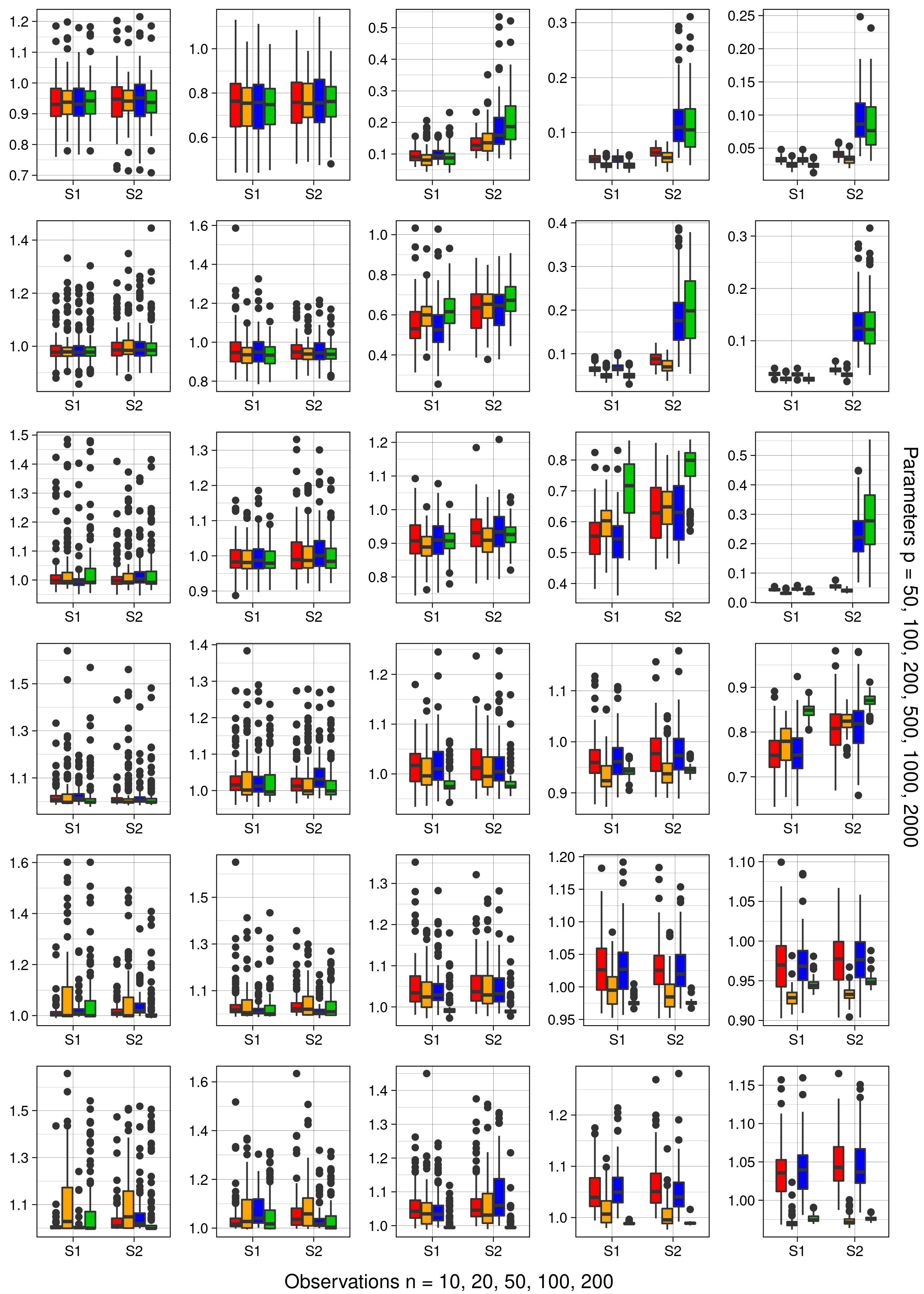
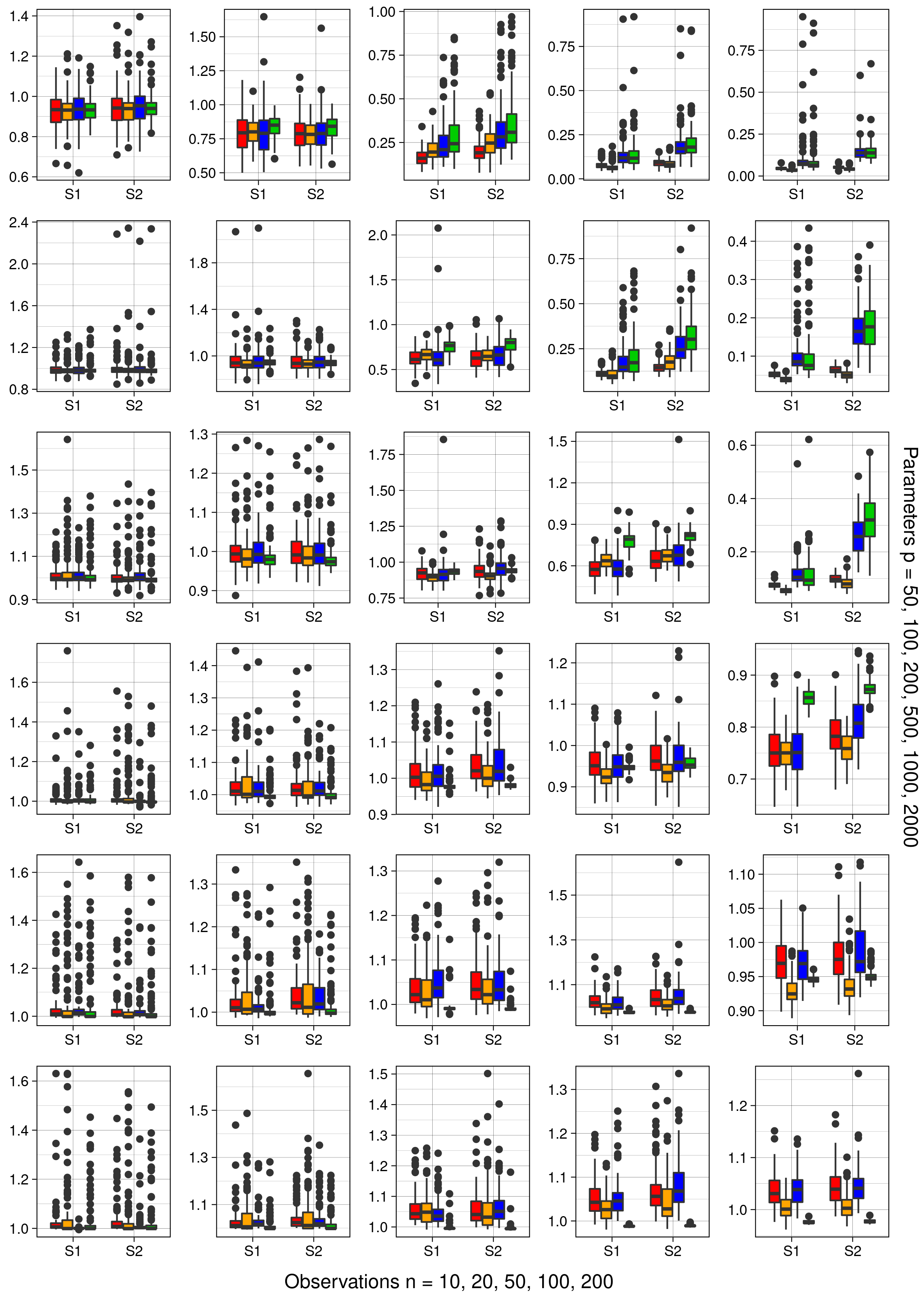
Robustness - it is clear from the upper right plots on Figure 1 that for Scenario 2 the robustness provided by the DPSS and DPHS models improves the predictive estimates of parameters when data is sufficient to make the model overdetermined, i.e. when is at least as large as . As expected, under Scenario 1 the results are similar for the models allowing heterogeneous and homogeneous variances. Interesting behaviour is observed when the model is underdetermined at varying degrees. When the model is highly underdetermined , models with the horseshoe priors provide more robust results in comparison to spike-and-slab priors. However, as approaches the spike-and-slab prior provides lower errors than the horseshoe (albeit at a smaller scale), until the model becomes overdetermined and the horseshoe prior models are preferred. Similar results are observed for the heavy tailed extension of the models. In contrast to the Gaussian models, when the models are at least determined the positive effect of robust variance modelling is less noticeable.
Coefficients - looking at Figure 1 and 2 from top to bottom the effect of adding coefficients to the model is illustrated on the predictive capabilities of the models. The Dirichlet process model performs well in the presence of heterogeneity, particularly as the number of model coefficients is less than the number of observations. The robustness added by the heterogeneous variances benefits the horseshoe prior in the overdetermined case and the spike-and-slab prior in the underdetermined case.
Clusters - one of the key advantages of the nonparametric approach we adopt is the availability of posterior densities for the number of variance components . The Dirichlet process’ assumption of a number of clusters which scale logarithmically towards infinity with can be observed by looking at the boxplots for samples of for an increasing in Figures 3 and 4 for the heavy tailed extension. A potentially useful caveat of the heavy tailed extension of the robust models is that the number of clusters increases at a slower rate than the case of Gaussian errors. In the case where a finite number of clusters in the data is known, or the number of clusters should scale faster or slower than logarithmically, priors that generalize the Dirichlet process can be used, e.g. the Pitman-Yor process (Pitman and Yor 1997). It is interesting to notice how, as the number of coefficients increases but the number of observations remain constant, the number of clusters retract themselves on their bias when the number of coefficients becomes much larger than the number of observations, as shown in Figures 5 and 6. A comparison of these two Figures also shows how the heavy tailed extension of the robust model provides a more gradual increase on the number of clusters .


4.2 Support Recovery
In addition to estimating the regression coefficients, a further task of interest, especially in high-dimensional regression, is to select a subset of attributes which are deemed significant for the predictive model. In a frequentist context, this is usually achieved via forward selection with sequential F-tests, or with or shrinkage and/or selection, for instance through the use of the AIC or BIC criteria.
One advantage of the Bayesian approach is that we can sample from the joint posterior of the coefficients, thus we can construct credible intervals with relative ease. In this section, we compare two methods for estimating the support of the regression model:
- •
The first approach is to simply look at the posterior of the inclusion parameter for selecting either the spike, or slab. Specifically, if the mode of the posterior is above level we add the index to the estimated support set . This method works only in the DPSS and SS models.
- •
The second approach is to look at the empirical posterior credible interval of at the percentiles and . If the constructed interval excludes zero, then we add the index to the estimated support set . This method is used for the DPHS and HS models.
We note that the second approach is somewhat similar to the z-cut method discussed in Ishwaran and Rao 2005, however, they construct a set where represents the posterior mean of the regression coefficients.
To summarise the performance of the two approaches, we take the number of true and false positive (, ) coefficients included in the model and consider how this changes as a function of . Clearly, these values will change as a function of , and in practice this may be tuned to favour either TP or FP results. For simplicity, we report results with . Table 1 summarises the performance of the posterior inclusion thresholding method for different values of in the heteroskedastic scenario (Scenario 2) and the standard Gaussian formulation of the models, similar results where observed on their heavy tailed extension. In the case of an overdetermined model, both the standard and robust implementations learn correctly the underlying data generating process. However, when the model is underdetermined the standard spike-and-slab tends to be more conservative in the inclusion of variables while the robust method favour a better estimate TP with the drawback of more FP. Similar results can be observed in the case of the horseshoe prior. The support recovery, or model selection, of the robust models will be detailed further when applied to real world data, where the benefits of each prior are illustrated.
| Model | n | 20 | 50 | 100 | 200 | ||||
|---|---|---|---|---|---|---|---|---|---|
| SS | TP | 5 | [0.95,8] | 14 | [12,14] | 14 | [14,14] | 14 | [14,14] |
| FP | 3 | [0,7] | 0 | [0,1] | 0 | [0,0] | 0 | [0,0] | |
| DPSS | TP | 5 | [2,8] | 14 | [12,14] | 14 | [14,14] | 14 | [14,14] |
| FP | 3 | [0.95,8] | 0 | [0,1] | 0 | [0,1] | 0 | [0,0] | |
| SS | TP | 4 | [1,10] | 17 | [1,25] | 28 | [28,28] | 28 | [28,28] |
| FP | 5 | [0,13.15] | 18 | [0,43.3] | 0 | [0,1] | 0 | [0,1] | |
| DPSS | TP | 4 | [1,9.05] | 20 | [14,26] | 28 | [28,28] | 28 | [28,28] |
| FP | 4 | [0,14] | 24 | [6.95,46.05] | 0 | [0,1] | 0 | [0,1] | |
| SS | TP | 4 | [0,18.15] | 25 | [0,51.05] | 31 | [1,56] | 56 | [56,56] |
| FP | 6 | [0,36.55] | 53 | [0,124.2] | 62 | [0,144] | 0 | [0,1] | |
| DPSS | TP | 3 | [0,12.1] | 42 | [16.95,56] | 54 | [47.9,56] | 56 | [56,56] |
| FP | 6 | [0,22] | 99 | [25.9,142.05] | 133 | [95.8,144] | 0 | [0,1] |
4.3 Reconstruction of transcription regulatory networks
We consider the problem of reconstructing genetic regulatory networks from gene expression data (Marbach et al. 2010). This problem can be modelled as a directed network, where each node corresponds to a different gene and each connection represents a directed interaction between two genes at the transcription level. The sparse spike-and-slab and horseshoe priors provide an attractive approach to reconstructing these networks using support recovery methods.
The models are tested on data from the challenge posed at the The Dialogue for Reverse Engineering Assessments and Methods (DREAM) 2009 conference, specifically the multifactorial subchallenge11 1 www.synapse.org/#!Synapse:syn3049712/wiki/74628. The challenge consists of reverse engineering five independent networks using 100 steady-state measurements for each network with 100 genes. The levels of expression of all the genes are measured under different perturbed conditions. Each gene for is treated independently and modelled through a linear relationship with the rest of the genes in the network , i.e. . Every has an independent spike-and-slab or horseshoe prior and is a normal random variable with mean zero and homogeneous variances in the case of SS and HS, or heterogeneous variances, in the case of DPSS and DPHS. For each gene, the support is recovered using the method described in Section 4.2 for the case of a spike-and-slab prior with . In the case of a horseshoe prior, we follow Steinke et al. 2007 and approximate the posterior probability of a connection from gene to gene by the probability of the event under the posterior for .
The performance of the different approaches is evaluated using the mean of the logarithmic loss of the probabilities of connections from gene to each gene , defined as
where if there is a directed connection from to and otherwise. Table 2 presents these results for each tested model. The improvement in prediction given by heterogeneous variances in the model is substantial. This supports the results from Section 4.2 on synthetic data, illustrating the improvement offered by robust models to correctly classify variables included in the model, specifically in their capability of reducing type II error in the predictions while correctly identifying the significant coefficients in the linear relationship. It is interesting to note that, while the DPSS model provided better support recovery results in the synthetic data example, the DPHS provides better results in the real data example of gene network reconstruction.
| SS | DPSS | HS | DPHS | |
|---|---|---|---|---|
| N1 | 0.1143 | 0.0948 | 0.0920 | 0.0854 |
| N2 | 0.1498 | 0.1380 | 0.1248 | 0.1173 |
| N3 | 0.1610 | 0.1158 | 0.1196 | 0.0900 |
| N4 | 0.1588 | 0.1118 | 0.1124 | 0.0970 |
| N5 | 0.1314 | 0.1095 | 0.1044 | 0.0933 |
5 Conclusion
This paper outlines a nonparametric extension of popular Bayesian variable selection models to account for heterogeneity, outliers and clustering effects. We also provide an extension to the model to allow for heavy-tailed data distributions. Fitting our Dirichlet process variable selection models is computationally efficient using a Gibbs sampling construction. The results presented for both synthetic and real data examples show a robust improvement in both predictive accuracy on test data and improved efficiency in identifying key model attributes.
This work could be further extended to encompass other variable selection models, including extensions of existing models, such as the regularized horseshoe model (Piironen et al. 2017). It would also be interesting to explore nonparametric priors that allow for more flexible assumptions on the expected clustering effect, such as the Pitman-Yor process (Pitman and Yor 1997).
References
- Aldous (1985) Aldous, D. J. (1985). “Exchangeability and related topics.” In École d’Été de Probabilités de Saint-Flour XIII—1983, 1–198. Springer.
- Bhattacharya et al. (2016) Bhattacharya, A., Chakraborty, A., and Mallick, B. K. (2016). “Fast sampling with Gaussian scale mixture priors in high-dimensional regression.” Biometrika, asw042.
- Breiman et al. (2001) Breiman, L. et al. (2001). “Statistical modeling: The two cultures (with comments and a rejoinder by the author).” Statistical science, 16(3): 199–231.
- Carpenter et al. (2017) Carpenter, B., Gelman, A., Hoffman, M. D., Lee, D., Goodrich, B., Betancourt, M., Brubaker, M., Guo, J., Li, P., and Riddell, A. (2017). “Stan: A probabilistic programming language.” Journal of statistical software, 76(1).
- Carvalho et al. (2009) Carvalho, C. M., Polson, N. G., and Scott, J. G. (2009). “Handling sparsity via the horseshoe.” In Artificial Intelligence and Statistics, 73–80.
- Carvalho et al. (2010) — (2010). “The horseshoe estimator for sparse signals.” Biometrika, 97(2): 465–480.
- Escobar and West (1995) Escobar, M. D. and West, M. (1995). “Bayesian density estimation and inference using mixtures.” Journal of the american statistical association, 90(430): 577–588.
- Ferguson (1973) Ferguson, T. S. (1973). “A Bayesian analysis of some nonparametric problems.” The annals of statistics, 209–230.
- George and McCulloch (1993) George, E. I. and McCulloch, R. E. (1993). “Variable selection via Gibbs sampling.” Journal of the American Statistical Association, 88(423): 881–889.
- Ghosal and Van der Vaart (2017) Ghosal, S. and Van der Vaart, A. (2017). Fundamentals of nonparametric Bayesian inference, volume 44. Cambridge University Press.
- Hjort et al. (2010) Hjort, N. J., Holmes, C., Muller, P., and Walker, S. G. (2010). Bayesian Nonparametrics. Cambridge University Press.
- Ishwaran and Rao (2005) Ishwaran, H. and Rao, J. S. (2005). “Spike and Slab Variable Selection: Frequentist and Bayesian Strategies.” The Annals of Statistics, 33(2): 730–773.
- Lo (1984) Lo, A. Y. (1984). “On a class of Bayesian nonparametric estimates: I. Density estimates.” The annals of statistics, 351–357.
- Makalic and Schmidt (2015a) Makalic, E. and Schmidt, D. F. (2015a). “A simple sampler for the horseshoe estimator.” IEEE Signal Processing Letters, 23(1): 179–182.
- Makalic and Schmidt (2015b) — (2015b). “A simple sampler for the horseshoe estimator.” IEEE Signal Processing Letters, 23(1): 179–182.
- Marbach et al. (2010) Marbach, D., Prill, R. J., Schaffter, T., Mattiussi, C., Floreano, D., and Stolovitzky, G. (2010). “Revealing strengths and weaknesses of methods for gene network inference.” Proceedings of the national academy of sciences, 107(14): 6286–6291.
- Mitchell and Beauchamp (1988) Mitchell, T. J. and Beauchamp, J. J. (1988). “Bayesian variable selection in linear regression.” Journal of the american statistical association, 83(404): 1023–1032.
- Piironen et al. (2017) Piironen, J., Vehtari, A., et al. (2017). “Sparsity information and regularization in the horseshoe and other shrinkage priors.” Electronic Journal of Statistics, 11(2): 5018–5051.
- Pitman and Yor (1997) Pitman, J. and Yor, M. (1997). “The two-parameter Poisson-Dirichlet distribution derived from a stable subordinator.” The Annals of Probability, 855–900.
- Steinke et al. (2007) Steinke, F., Seeger, M., and Tsuda, K. (2007). “Experimental design for efficient identification of gene regulatory networks using sparse Bayesian models.” BMC systems biology, 1(1): 1–15.