A look at Representations of through the Lens of Size
Abstract.
How to study a nice function on the real line? The physically motivated Fourier theory technique of harmonic analysis is to expand the function in the basis of exponentials and study the meaningful terms in the expansion. Now, suppose the function lives on a finite non-commutative group , and is invariant under conjugation. There is a well-known analog of Fourier analysis, using the irreducible characters of . This can be applied to many functions that express interesting properties of . To study these functions one wants to know how the different characters contribute to the sum?
In this note we describe the case of the theory we have been developing in recent years which attempts to give a fairly general answer to the above question for finite classical groups.
The irreducible representations of are “well known” for a very long time [Frobenius1896, Jordan1907, Schur1907] and are a prototype example in many introductory courses on the subject. We are happy that we can say something new about them. In particular, it turns out that the representations that were considered as “anomalous” in the ”old” point of view (known as the ”philosophy of cusp forms”) are the building blocks of the current approach.
To Joe Wolf mazal tov ad me’ah v’esrim
0. Introduction
An important invariant attached to any finite group is its representation ring [Zelevinsky81]
i.e., the ring generated from the set of isomorphism classes of irreducible representations (irreps) using the operations of addition and multiplication given, respectively, by direct sum and tensor product
The main goal of this note is to advertise, using the special linear group over the finite field with odd elements
our recent discovery [Gurevich-Howe15, Gurevich-Howe17, Gurevich17, Howe17-1, Howe17-2] that in the case that is a finite classical group the ring has a natural ”tensor rank” filtration that encodes the analytic properties of the representations. In particular, moving to the associated graded pieces, each member of the unitary dual gets a well defined non-negative integer called tensor rank and denoted This integer seems—see Figure 1 for illustration11 1 The numerics in this note were generated using the computer algebra system Magma. in the case of —to be intimately related to analytic properties of such as its dimension and size of character values.

In the rest of the introduction we discuss two aspects of the tensor rank filtration. The first is the fact that this is the first point of view that makes the degenerate discrete and principal series representations of seem significant rather than anomalous. The second aspect we discuss, through a specific example for is the potential usefulness of the tensor rank filtration to the harmonic analysis of the finite classical groups.
0.1. Degenerate Discrete and Principal Series Representations
Let be the group of -rational points of a reductive algebraic group defined over The Gelfand–Harish-Chandra ”philosophy of cusp forms” [Gelfand62, Harish-Chandra70] asserts that each member of can be realized, in some effective manner, inside the induction from a cuspidal representation (i.e., one that is not induced from a smaller parabolic subgroup) of a parabolic subgroup of
The above philosophy is a central one and leads to important developments in representation theory of reductive groups over local and finite fields, in particular the work of Deligne–Lusztig [Deligne-Lusztig76] on the construction of representations of finite reductive groups and Lusztig’s striking achievement: The classification [Lusztig84] of these representations.

Let us see how this philosophy manifests itself in the cases when is or -see Figure 2 (let us ignore for this discussion the one dimensional representations). In both cases around of the irreps are cuspidals, i.e., and form the so called discrete series, and are the so called principal series, i.e., induced from the Borel subgroup of upper triangular matrices in Moreover, it is well known, and not so difficult to show [Fulton-Harris91], that the discrete and principal series representations of can be obtained by restriction from the corresponding irreps of These restrictions are typically irreducible, with only two exceptions: One discrete series representation of dimension and one principal series representation of dimension split into two pieces. Hence one has—see Figure 2—two discrete and two principal series representations of dimensions and , respectively. These representations are called in the literature ”degenerate discrete series” and ”degenerate principal series” and are usually treated as anomalous.
In this note we show that the tensor rank filtration proposes a quantitative measurement that, in particular, demonstrates that the degenerate representations are significant rather then anomalous. In fact, in some formal sense these irreps are the ”atoms” of the all theory of ”size” of representations we are describing.
0.2. Harmonic Analysis on a Finite Group
Suppose we want to study a class function , defined on a finite group :
for every
Many interesting examples of present similar manner discussed below.
0.2.1. The problem of harmonic analysis on a finite group
Class functions can, in principle, be investigated using the representation theory of : it is a basic fact [Serre77] that one can expand them as a linear combination of the irreducible characters of . This is the harmonic analysis approach for studying class functions on In particular, this technique can be applied to many functions that express interesting properties of [Diaconis88, Guralnick-Malle14, Liebeck17, Liebeck-O’Brien-Shalev-Tiep10, Malle14, Shalev07, Shalev17]. In that latter case the expansion is in many cases of the form
where stands for some relevant expression in terms of the character ratios of the irreps of
The above discussion suggests the following:
Problem (Main problem of harmonic analysis on ). Estimate the character ratios
and possible relations among them.
0.2.2. Example: The commutator mapping on
Consider the group and the commutator mapping
| (0.1) |
For an element let us denote by the set called the fiber over of the commutator mapping. We are interested in the distribution of the number of elements when runs in the set It is natural [Shalev07] to make a suitable normalization and study the class function
| (0.2) |
To see how this function behaves over the various conjugacy classes of , let us recall [Fulton-Harris91] that has conjugacy classes with standard representatives
| (0.3) |
where is a non-square22 2 For the rest of this note stands for a non-square element of , and

Using numerics—see Figure 3 for illustration—one can suspect the following to be true:
Theorem (Uniformity of the commutator map). We have33 3 For numerical sequences we write if there is s.t. for all sufficiently large
| (0.4) |
The relevant formula enabling the representation theoretic study of the function is due to Frobenius [Frobenius1896]
| (0.5) |
Looking back on (0.4), and taking into account the trivial representation in (0.5), we see that to verify the uniformity statement above we need to
- Goal:
-
Explore the cancellation
(0.6)
In fact, it is possible (see [Garion-Shalev09]) to verify (0.6) invoking available character tables of [Fulton-Harris91]. There are two drawbacks to this approach. First, it will prevent us from telling the story we are trying to make. Second, and more seriously, it is not really feasible to have explicit character tables for more complicated groups, e.g., the high rank symplectic groups. This is a family that contains as a member and for which one might expect (see the numerics in [Gurevich-Howe15]) similar behavior of the relevant Frobenius sum (0.6). So we would like to have a different approach to achieve the goal (0.6). In this note we demonstrate, in the case of how the tensor rank filtration might assists with that task.
Acknowledgements. This note was written in the winter of 2017-18 while S.G. was visiting the Mathematics Departments at Weizmann Institute and Yale University, and the College of Education at Texas AM University, and he would like to thank these institutions, personally H. Naor and O. Sarig at Weizmann, D. Altschuler, C. Villano, and I. Frenkel at Yale, and R. Howe at TAMU. We also want to thank S. Goldstein and J. Cannon for their help with numerical aspects of the project, part of it is reported here.
1. Character Ratios and Tensor Rank
A priori, it is possible that the sum (0.6) is small as it is because each of the (around) terms there is so small. This is not the case.
1.1. Character Ratios
A quick numerical experiment with Magma tells us (see Figure 4 for the outcome) that indeed the sum (0.6) is small due to cancellations. For example,

in the last two rows of the second column of Figure 4 there are around character ratios each one of order of magnitude Moreover, looking again on the second and third rows of the second column, one hope for two ”sub-cancellations” in the sum (0.6), one between the character ratios of the irreps of dimensions and another one between the character ratios of the other irreps.
We will show that indeed this what is going on.
1.2. Tensor Rank of a Representation
The different orders of magnitude of the character ratios discussed above—see also Figure 1 for illustration—is a manifestation of a particular invariant—called tensor rank—that can be attached to any representation of and should be regarded in a formal sense as its ”size”.
Let be a non-negative integer and consider the collection of representations in that appear inside sums (with integer coefficients) of -fold, , tensor product of the four irreps of of dimensions One has , and , so the ’s form a filtration of that we call tensor rank filtration. In fact,
Proposition 1.2.1.
We have
Now we can pass to the associated graded pieces and in particular obtain a well defined notion of tensor rank for representations [Gurevich-Howe17]. Concretely,
Definition 1.2.2 (Tensor rank).
Let be a representation of We say that has tensor rank denoted if
Let us denote by the family of irreps of tensor rank Combining Proposition 1.2.1 and the information appearing in Figure 2 we see that consists of the trivial representation, is the collection of irreps of dimensions , and finally is the family of irreps of dimensions and
Going back to the problem of exploring the cancellation in the sum (0.6) our idea is to split it over the tensor ranks
and to witness the cancellation in each partial sum. Of course, for this we will need more information on the irreps of each given tensor rank.
2. The Heisenberg and Oscillator Representations
Where do the tensor rank one irreps of come from? A. Weil shed some light on this in [Weil64]. They can be found by considering the Heisenberg group.
2.1. The Heisenberg Group
We consider the vector space of column vectors of length with entries in . We equip with the non-degenerate skew-symmetric bilinear form
where is the row vector transpose of , and is the identity matrix. The pair is called symplectic vector space.
The Heisenberg group attached to is a two-step nilpotent group that can be realized by the set
with the group law
In particular, the center of the Heisenberg group
is equal to its commutator subgroup.
2.2. Representations of the Heisenberg Group
We would like to describe the irreps of the Heisenberg group.
Take an irreducible representation of . Then, by Schur’s lemma [Serre77], the center will act by scalars
where is the the identity operator on the representation space of , and is a character of called the central character of . If then factors through , which is abelian, so is itself a character of The case of non-trivial central character is described by the following celebrated theorem [Mackey49]:
Theorem 2.2.1 (Stone–von Neumann–Mackey).
Up to equivalence, there is a unique irreducible representation with given non-trivial central character in
We will call the (isomorphism class of the) representation the Heisenberg representation associated to the central character
Remark 2.2.2 (Realization).
There are many ways to realize (i.e., to write explicit formulas for) [Gerardin77, Gurevich-Hadani07, Gurevich-Hadani09, Howe73-1, Weil64]. In particular, it can be constructed as induced representation from any character extending to any maximal abelian subgroup of . To have a concrete one, note that the inverse image in of any maximal subspace of on which is identically zero (a.k.a. Lagrangian) will be a maximal abelian subgroup for which we can naturally extend the character . For example, consider the Lagrangian
| (2.1) |
and the associated maximal abelian subgroup with character on it, given by
Then we have the explicit realization of given by the action of by right translations, on the space
| (2.2) |
In particular, we have
2.3. The Oscillator Representation
Consider the group of automorphism of that preserve the form . The action of on lifts to an action on by automorphisms leaving the center point-wise fixed. The precise formula is It follows from the Stone–von Neumann–Mackey theorem, that the induced action of on the set will leave fixed each isomorphism class This means that, if we fix a vector space realizing then for each in there is an operator that acts on space and satisfies the equation
| (2.3) |
Note that, by Schur’s lemma, the operator is defined by (2.3) up to scalar multiples. This implies that for any we have where is an appropriate complex number of absolute value . It is well known (see [Gerardin77, Gurevich-Hadani07, Gurevich-Hadani09] for explicit formulas) that over finite fields of odd characteristic the mapping can be defined so that for every , i.e., defines a representation of We summarize:
Theorem 2.3.1 (Oscillator representation).
There exists44 4 This representation is unique except the case and where there is a canonical one [Gurevich-Hadani07, Gurevich-Hadani09]. a representation
| (2.4) |
that satisfies the identity (2.3).
We will call the oscillator representation. This is a name that was given to this representation in [Howe73-1] due to its origin in physics [Segal60, Shale62]. Another popular name for is the Segal–Shale–Weil or just Weil representation, following the influential paper [Weil64].
Remark 2.3.2 (Schrödinger model).
We would like to have some useful formulas for . We consider the Lagrangian decomposition , where is the first coordinates Lagrangian (2.1) and is the second coordinates Lagrangian defined similarly. In terms of this decomposition, the space (2.2) is naturally identified with
| (2.5) |
On the space (2.5) we realize the representation . This realization is sometime called the Schrödinger model [Howe80]. In particular, in that model for every we have [Gerardin77, Gurevich-Howe15, Weil64]
(A)
where is symmetric;
(B)
where is symmetric, and the quadratic Gauss sum [Ireland-Rosen90];
(C)
where its transpose inverse, and is the Legendre symbol55 5 For the Legendre symbol or according to being a square or not, respectively..
It turns out that the isomorphism class of does depends on the central character in However, this dependence is weak. The following result [Gerardin77, Howe73-1, Howe73-2] indicates that there are only two possible oscillator representations. For a character in denote by the character
Proposition 2.3.3.
We have iff for some
2.4. The Representations of Tensor Rank One
The oscillator representations are slightly reducible. Indeed, for any two representations of any group one has the intertwining number . The following is well known [Gerardin77, Howe73-1, Howe82].
Proposition 2.4.1.
We have
The meaning of Proposition 2.4.1 is that has two irreducible pieces. They can be computed explicitly as follows. The center acts on the representation , inducing the decomposition into irreps
| (2.6) |
where is the subspace of vectors on which acts trivially, and is the subspace of vectors on which acts via the sign character. Moreover, using the description for the action of given in Remark 2.3.2 (C), it is easy to verify that for odd
and for even
Now, substituting we have and using the two possible oscillator representations (see Proposition 2.3.3) we obtain all the irreps of tensor rank one. These have dimensions . They are exactly the representations that appear ”anomalous” in the philosophy of cusp forms—see Section 0.1.
Next, we want information on the tensor rank two irreps.
3. The eta Correspondence
How to get information on the tensor rank two irreps of ? This section will include an answer to this question. In fact, we introduce a systematic method called -correspondence that works uniformly for all tensor ranks generalizes the construction of tensor rank one irreps described in Section 2, and exists for all classical groups over finite and local fields [Gurevich-Howe15, Gurevich-Howe17, Howe17-1, Howe17-2].
3.1. The Dual Pair
Consider the vector space and let be an inner product (i.e., a non-degenerate symmetric bilinear form) on . The pair is called a quadratic space. In this note we will be interested only in the cases In these cases we have the following examples:
- •
: The zero space with
- •
: The line with the form or with the form where is a non-square in .
- •
: The plane with
- –
the form . In this case—called hyperbolic plane—i.e., there are two lines on which the form is identically zero.
- –
the form where is a non-square in . In this case—called anisotropic plane—there is no line on which the form is identically zero.
- –
It is well known [Lam05] that up to isometry there are only two quadratic spaces of dimension over In particular, for the above list of examples is exhaustive.
Finally, for a quadratic space we denote by the associated isometry group and call it the orthogonal group. We might also denote this group by or according as the form is, respectively, or or by to mean either one of these groups.
Now, let us take the plane with the symplectic form
and consider the vector space —the tensor product of and [Atiyah-Macdonald69]. It has a natural structure of a symplectic space, with the symplectic form given by The groups and act on via their actions on the first and second factors, respectively,
Both actions preserve the form and moreover the action of commutes with that of , and vice versa. In particular, we have a map
| (3.1) |
that embeds each of the two factors and in and the two images form a pair of commuting subgroups. In fact, each is the full centralizer of the other inside Thus, the pair forms what has been called in [Howe73-1] a dual pair of subgroups of .
3.2. The eta Correspondence
Let us fix for the rest of this paper a non-trivial character of Consider the symplectic space with the form described in Section 3.1 above. In this setting, we have the oscillator representation of given by (2.4).
Note that for is the trivial representation, and for it is, respectively, the oscillator representation or of , according as the form is or
Proposition 3.2.1.
Assume that . As a representation of
, in case the form is we have
| (3.2) |
and in case is we have
| (3.3) |
For the rest of this note, if not otherwise stated, we assume that the dimension of is or Note that, by Proposition 3.2.1, every representation of that appears in is of tensor rank . Let us denote by the -spectrum of in , i.e., the subspace of consisting of the isotypic components of tensor rank irreps of The group algebras act on . Let us denote by the irreps of of tensor rank The following is a key result:
Theorem 3.2.2 (-correspondence).
We have
We call (3.4) the eta correspondence.
In [Gurevich-Howe15, Gurevich-Howe17], following initial ideas from [Howe73-1], we introduced techniques proving Theorem 3.2.2 in generality for any dual pair when one of the members is moving in a Witt tower.
In this note we offer more elementary and explicit verification.
3.3. Explicit Description of the eta Correspondence
We are interested in getting information on the restriction of the oscillator representation of to Consider the intertwining number . In case of we know (see Proposition 2.4.1 for ) that this number is and , respectively.
Proposition 3.3.1.
Suppose Then,
| (3.5) |
Now, we consider the restriction, i.e., the pullback via the map (3.1), of to the product We decompose this restriction into isotypic components for
| (3.6) |
where is a representation of
We want now to make the decomposition (3.6) explicit. In most cases is equal to , however, there are cases when is a proper sub-representation, and cases when does not contribute to the -spectrum at all.
In case we make the convention and so and the trivial representation.
3.3.1. The - decomposition
Let us denote by the two oscillator representations of in the cases that is equipped with the forms , respectively. The orthogonal groups act on the representations respectively. In these cases the isotypic components in (3.6) are and where are the trivial and sign representations of and are the four irreps that we discussed in Section 2.4. In particular, in these cases , and we verified Theorem 3.2.2 explicitly.
3.3.2. The - decomposition
We first recall some information on the orthogonal groups and their irreps, and then we describe the decomposition (3.6) associated with these groups.
The irreps of
The groups fit into a short exact sequence
| (3.7) |
where the third morphism is , and stand for the special orthogonal groups. It might be convenient for us to choose a splitting of (3.7), i.e., to consider a reflection
| (3.8) |
Then and for every Moreover, the groups are cyclic with and - the norm one elements in a quadratic extension of . In particular, and
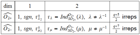
Let us recall the irreps of —see Figure 5 for a summary. There are of them and they can be realized as follows. For every character of we consider the induced representation
| (3.9) |
Note that
- •
for each
- •
(3.8) induces an isomorphism , where
- •
In particular, the ’s with give the irreps of dimension In addition, there are irreps of dimension : The trivial representation , the sign character , and the two components of on which the reflection (3.8) acts66 6 The notation depends on If is another reflection, then for unique by or , respectively, where is the unique non-trivial character of such that
The irreps of are described in the same manner starting with of them of dimension induced from characters , of etc.—see Figure 5 for the outcome in this case.
The decomposition

Proposition 3.3.2 (The decomposition).
Every representation , appears in and in that range the corresponding representations of (3.6) are irreducible and pairwise non-isomorphic. In particular, Part (1) of Theorem 3.2.2 holds true. Moreover, for the description of and we have
- (1)
The representation is of tensor rank and dimension We denote it by or by since it is known as the Steinberg representation.
- (2)
The representations , are of tensor rank and dimension . We denote them by .
- (3)
The representations are the two tensor rank irreps of dimension
Parts (1) and (2) of Proposition 3.3.2 give an explicit description of the eta correspondence (3.4).
Next, we treat the case—see Figure 6 (left) for a summary.
Proposition 3.3.3 (The decomposition).
Every representation appears in . Moreover, for the description of and we have
- (1)
The representation where is the Steinberg representation of tensor rank and dimension . We denote it by In addition, .
- (2)
The representations are irreducible, pairwise non-isomorphic, of tensor rank and dimension . We denote them by .
- (3)
The representations are the two tensor rank irreps of dimension
Parts (1) and (2) of Proposition 3.3.3 give an explicit description of the eta correspondence (3.4).
Remark 3.3.4 (Double commutatnt property).
Note the difference between the two decompositions appearing in Propositions 3.3.2 and 3.3.3. In the first case and generate each other’s commutant when acting on the space . This is not what is happening in the second case of and However, they do generate each other’s commutant—see Figure 6 (left)—after taking away from the isotypic component of the trivial representation of
3.3.3. Summary
The -correspondence that was described explicitly in this section, gives a way to realize irreps of . It does it for each tensor rank separately. The realization is inside specific oscillator representations, and in each one is described in term of irreps of corresponding orthogonal groups. In particular, , and , verifying Part (2) of Theorem 3.2.2. Finally, by counting so which verifies Proposition 1.2.1.
4. Application to Uniformity of the Commutator Map
We go back to the problem of the uniformity of the commutator map described in Section 0.2.2 for .
4.1. Statement
We considered the function on given by (0.2) , i.e., the normalized cardinality of the fiber over of the map
We wanted to show that,
Theorem 4.1.1.
For we have
| (4.1) |
4.2. Verifying Cancellations in Frobenius’s Character Sum
Recall that Frobenius’s Formula (0.5) gives a representation theoretic interpretation of as a character sum
| (4.2) |
In Section 1 we looked on (4.1) and (4.2) and since—see Figure 4—around of the summands in (4.2) are of size we understood that we need to verify cancellations in the sum on the right-hand side of (4.2). Moreover, we noticed that for some elements the size of the summands in (4.2) seem—see Figure 4—larger for irreps of tensor rank then for these of tensor rank . Hence, at the end of Section 1 we proposed to verify the cancellations in (4.2) by splitting the sum into two partial sums, one over tensor rank one irreps and one over tensor rank two irreps
and explore cancellations within each sub-sum.

The numerics appearing in Figure 7 suggest that the above idea might work. Indeed, using the information on and supplied by the -correspondence, we can show that
Proposition 4.2.1.
Let . We have
| (4.3) |
and
| (4.4) |
4.3. Proof of Proposition 4.2.1
The -correspondence enables to relate the sums (4.3) and (4.4) that we want to estimate, to some other sums that we can actually compute using only two inputs: The character of the oscillator representation, for which we have explicit formulas [Gerardin77, Gurevich-Hadani07, Howe73-1, Howe73-2, Issacs73, Teruji08]; and the character of the Steinberg representation, for which a simple description is known [Fulton-Harris91].
Let us denote by the characters of the two oscillator representations of associated with a character of (see Section 3.3.1). The formulas (see loc. sit.) in particular give:
Fact 4.3.1.
For we have
- (1)
The oscillator characters satisfies,
(4.5) where is the usual quadratic Gauss sum [Ireland-Rosen90], is the Legendre symbol, and means in the same conjugacy class.
- (2)
The Steinberg Character satisfies,
(4.6) where is the collection of lines in the plane that are fixed by .
The tensor rank one sum
First, we estimate the sum (4.3) for .
Let us write where and denote the characters of the components of of dimensions and respectively, and likewise
and, moreover, from the definition of and and Formula (4.5), we get
| (4.12) |
So overall, by a combination (4.7), (4.8), and (4.12), we have
where
This completes a quantitative form of (4.3).
The tensor rank two sum
Next, we estimate the sum (4.4) for . It has a similar structure to
Using the explicit description of the -correspondence—see Figure 6—we have
| (4.13) | |||||
We would like to estimate the various terms in (4.13).
Consider the sums and above. Denote by and respectively, the anisotropic and hyperbolic planes, and by respectively, the characters of the oscillator representations of the groups (see Section 3.2). Then,
where the first equality follows from the explicit descriptions of appearing in Figure 6, and the second equality follows from a combination of Proposition 3.2.1 and Formula (4.5). So, together with (4.8) we get,
| (4.15) |
Next, concerning the term in (4.13). From the explicit description of appearing in Figure 6, we obtain
| (4.16) |
So, using Formulas (3.3), (4.5), and (4.12), (4.6), inserted in (4.16), we get
| (4.17) |
where .
This is a quantitative form of (4.4).
Appendix A The Weyl transform
Let us denote by a vector space supporting the Heisenberg representation of the Heisenberg group defined in Section 2.2. Various calculations done in this note involve the space of all linear transformation on Interestingly, this operator space has an invariant description [Gurevich-Hadani07, Howe73-1] that was discovered by Weyl in the context of quantum mechanics [Weyl27].
A.1. Definition of the Weyl Transform
Consider the vector space of complex valued functions on the symplectic space Then, we have a canonical isomorphism, called the Weyl transform,
| (A.1) |
for every
Here is a useful application of the Weyl transform (A.1).
A.2. Application for Intertwining Numbers
We describe application for the computation of intertwining numbers for restrictions of the oscillator representation to subgroups Note that the identification intertwines the conjugation action of on with its permutation action on Consider the intertwining number i.e., the dimension of the space of operators on that commute with the action of Denote by the set of orbits for the action of on It follows
Corollary A.2.1.
We have
Appendix B The Double Commutant Theorem
B.1. Formulation
For the convenience of the reader, here is the statement.
Theorem B.1.1 (Double commutant theorem).
Let be a finite dimensional vector space. Let be two sub-algebras, such that
- (1)
The algebra acts semi-simply on
- (2)
Each of and is the full commutant of the other in
Then acts semi-simply on and as a representation of we have
| (B.1) |
where are all the irreducible representations of , and are all the irreducible representations of In particular, we have a bijection between irreducible representations of and and moreover, every isotypic component for is an irreducible representation of
On the other hand, if commute and as a representation of the decomposition (B.1) holds, then each of and is the full commutant of the other in
Appendix C Proofs
C.1. Proof of Proposition 2.4.1
Proof.
Take in Corollary A.2.1 and note as claimed.
C.2. Proof of Proposition 3.2.1
Proof.
Let us denote by the oscillator representation associated with a symplectic vector space and a central character It is well known that and for every and two symplectic spaces ,
Next, in the case endowed with the form we can identify as a -space, with and in the case is with form we can identify as a -space, with where a non-square.
C.3. Proof of Proposition 3.3.1
Proof.
We take and in Corollary A.2.1, and compute We identify the action of on with its diagonal action on , and find that the orbits are
- •
For each the orbit
- •
For each the orbit
- •
The orbits
So, overall we have orbits, as claimed.
C.4. Proof of Propositions 3.3.2 and 3.3.3
Proof.
We give a proof that works more or less in a uniform manner for both groups .
The verification will use a realization of which is convenient for the groups Indeed, can be realized on the space in such a way that for it is its permutation representation. To arrive to this realization, write and consider the associated Lagrangian decomposition . Then we have the Schrödinger model (see Remark 2.3.2) realizing as described above.
Recall that by Witt’s theorem [Lam05] the groups act transitively on the each of the sets of vectors with a given value for the inner product. To see what representations of appear in we decompose
and study the spaces .
Let us start with the non-isotropic orbits, i.e., , . The stabilizer subgroup of a non-isotropic vector is the orthogonal group of the orthogonal complement of the line spanned by , i.e., the group generated by the reflection with respect to that line. In particular, the groups act simply transitively on ,
It follows that the character can not appear in since it would have to be represented by the constant function by transitivity of , but this transforms by the identity character of .
For the characters of that are non-trivial on , one will take value on a given reflection, and one will take value . Clearly, only the one that takes value on the reflection that stabilizes the vector can live on the orbit. That means that each of these characters live on half of the orbits of non-isotropic vectors.
Finally, it is easy to see that each of the two-dimensional irreps of appear once in , .
For the double commutant property for we know from the above analysis that every irrep but appears in , so by Plancherel [Serre77] it gives linearly independent operators in the the commutant so by (3.5) it gives the all commutant.
In summary, the isotypic components in of irreps of are
- •
, with (note that for ), so
- •
pairwise non-isomorphic with
- •
two non-isomorphic irreps with
This completes the Proof of Proposition 3.3.2.
Consider the group note that it acts simply transitively on the non-zero isotropic vectors, so the representation of on is the direct sum of the trivial representation and the regular representation. So contains the representation once, the trivial representation twice, the two characters of which are non-trivial on each once, and each of the two-dimensional irreps of twice.
For the double commutant property for , we have all irreps appearing, but they only give operators, so by (3.5) we are missing
We will show that
Lemma C.4.1.
The isotypic component in of the trivial representation of is two-dimensional on which acts by .
This means that only supplies two of the four operators in the commuting algebra for this component. So if we leave out the trivial representation of , then we need only operators. On the other hand, from Lemma C.4.1 and the analysis we have already done above we see that, on the complement of the trivial representation of we get all the representations of except , so this supplies operators, which is the needed number.
In summary, this will show that the isotypic components in of irreps of are
- •
.
- •
- •
pairwise non-isomorphic with
- •
two non-isomorphic irreps with
To prove Lemma C.4.1 it is enough, due to our knowledge on the size of the commutant, to show that sits inside the -invariant subspace of To show this, we will use another realization of , that helps to visualize the action of Decompose into a direct sum of isotropic lines. This induces the Lagrangian decomposition , that we can further identify with . In particular, we can realize on the space where
- (1)
The action of is its permutation representation.
- (2)
The action of is identified with the scaling action of
- (3)
The action of the reflection is via the symplectic Fourier transform given by
for every ,
References
- [Atiyah-Macdonald69] Atiyah M. and Macdonald I., Introduction to Commutative Algebra. Addison-Wesley (1969).
- [Deligne-Lusztig76] Deligne P. and Lusztig G., Representations of reductive groups over finite fields. Annals of Math. 103 (1976), 103-161.
- [Diaconis88] Diaconis P., Group representations in probability and statistics. IMS Lecture Notes Monogr. Ser. vol. 11 (1988).
- [Fulton-Harris91] Fulton W. and Harris J., Representation theory: A first course. GTM 129, Springer (1991).
- [Frobenius1896] Frobenius F.G., Über Gruppencharaktere. Sitzber. Preuss. Akad. Wiss. (1896) 985–1021.
- [Gelfand62] Gelfand, I. M., Automorphic functions and the theory of representations. Proceedings of ICM, Stockholm (1962), 74–85.
- [Gerardin77] Gérardin P., Weil representations associated to finite fields. J. Alg. 46 (1977), 54-101.
- [Garion-Shalev09] Garion S. and Shalev A., Commutator maps, measure preservation, and -systems. Transactions of the American Mathematical Society 361 (2009), 4631–4651.
- [Guralnick-Malle14] Guralnick R. and Malle G., Rational rigidity for . Comp. Math., v.150 (2014).
- [Gurevich-Hadani07] Gurevich S. and Hadani R., The geometric Weil representation. Selecta Math. 13 (2007), 465-481.
- [Gurevich-Hadani09] Gurevich S. and Hadani R., Quantization of Symplectic Vector Spaces over Finite Fields. Journal of Symplectic Geometry, Vol. 7, N. 4 (2009), 475-502.
- [Gurevich-Howe15] Gurevich S and Howe R., Small Representations of finite classical groups. Proceedings of Howe’s 70th birthday conference, New Haven (2015).
- [Gurevich-Howe17] Gurevich S and Howe R., Rank and Duality in Representation Theory. Takagi lectures Vol. 19, Japanese Journal of Mathematics (2017) 67-100.
- [Gurevich17] Gurevich S., Small Representations of finite Classical Groups. Special Lecture at IAS, March 8, 2017: https://video.ias.edu/specialrep/2017/0308-ShamgarGurevich.
- [Harish-Chandra70] Harish-Chandra., Eisenstein series over finite fields. Functional analysis and related fields, Springer (1970), 76–88.
- [Howe73-1] Howe R., Invariant theory and duality for classical groups over finite fields with applications to their singular representation theory. Preprint, Yale University (1973).
- [Howe73-2] Howe R., On the character of Weil’s representation. Tran. AMS 177 (1973), 287-298.
- [Howe77] Howe R., -series and invariant theory. Proc. Sympos. Pure Math., Corvallis, Ore. (1977), 275-285.
- [Howe80] Howe R., On the role of the Heisenberg group in harmonic analysis. Bull. AMS 3 (1980), N. 2, 821-843.
- [Howe82] Howe R., On a notion of rank for unitary representations of the classical groups. Harmonic analysis and group representations, Liguori, Naples (1982), 223-331.
- [Howe17-1] Howe R., On the role of rank in representation theory of the classical groups. Special Lecture at IAS, March 8, 2017: https://video.ias.edu/reptheory/2017/0308-RogerHowe.
- [Howe17-2] Howe R., Rank and Duality in Representation Theory. The 19th Takagi Lectures: http://www.kurims.kyoto-u.ac.jp/˜toshi/jjm/JJM_HP/contents/takagi/takagi-video.htm.
- [Issacs73] Isaacs I.M., Characters of solvable and symplectic groups. Amer. J. Math. 95 (1973), 594-635.
- [Ireland-Rosen90] Ireland K. and Rosen M., A Classical Introduction to Modern Number Theory. Springer (1990).
- [Jordan1907] Jordan H.E., Group-characters of various types of linear groups. Amer. J. Math. 29 (1907), 387-405.
- [Lam05] Lam T.Y., Introduction to Quadratic Forms over Fields. American Mathematical Society (2005).
- [Liebeck17] Liebeck M.W., Character ratios for finite groups of Lie type, and applications. Finite Simple Groups: Thirty Years of the Atlas and Beyond, CM 694 AMS (2017), 193-208.
- [Liebeck-O’Brien-Shalev-Tiep10] Liebeck M.W., O’Brien E.A., Shalev A., and P. H. Tiep., The Ore conjecture. JEMS 12 (2010), 939-1008.
- [Lusztig84] Lusztig, G., Characters of Reductive Groups over a Finite Field. Annals of Math. Studies, Princeton University Press (1984).
- [Mackey49] Mackey G.W., A theorem of Stone and von Neumann. Duke Math. J. 16 (1949), no. 2, 313–326.
- [Malle14] Malle G., The proof of Ore’s conjecture. Sém. Bourbaki, Astérisque 361 (2014), 325-348.
- [Schur1907] Schur I., Untersuchungen über die Darstellung der endlichen Gruppen durch gebrochene lineare Substitutionen. Journal für die reine und angewandte Mathematik 132 (1907), 85–137.
- [Segal60] Segal, I.E., Lectures at the 1960 Boulder Summer Seminar, AMS, Providence, RI.
- [Serre77] Serre J.P., Linear Representations of Finite Groups. Springer (1977).
- [Shalev07] Shalev A., Commutators, Words, Conjugacy Classes and Character Methods. Tur. J Math 31 (2007), 131-148.
- [Shalev17] Shalev A., Conjugacy classes, growth and complexity. Finite Simple Groups: Thirty Years of the Atlas and Beyond, CM 694 AMS (2017), 209-222.
- [Shale62] Shale D., Linear symmetries of free boson fields. Trans. AMS 103 (1962), 149-167.
- [Teruji08] Teruji T., The character of the Weil representation. J. Lon. Math. Soc. (2008) 77, 221-239.
- [Weil64] Weil A., Sur certains groups d’operateurs unitaires. Acta Math. 111 (1964), 143-211.
- [Weyl27] Weyl H., Quantenmechanik und Gruppentheorie. Zeitschrift für Physik, Vol. 46, Issue 1-2 (1927), 1-46.
- [Weyl46] Weyl H., The classical groups, their invariants and representations. Princeton Univ. Press (1946).
- [Zelevinsky81] Zelevinsky A., Representations of finite classical groups: A Hopf algebra approach. LNM 869. Springer (1981).