The Bluedisk survey: thickness of Hi layers in gas rich spiral galaxiesJournal: ApJ
Abstract
We use an empirical relation to measure the Hi scale height of relatively Hi rich galaxies using 21-cm observations. The galaxies were selected from the BLUEDISK, THINGS and VIVA surveys. We aim to compare the thickness of the Hi layer of unusually Hi rich with normal spiral galaxies and find any correlation between the Hi scale height with other galaxies properties. We found that on average the unusually Hi rich galaxies have similar Hi disk thickness to the control sample and the galaxies selected from the THINGS and VIVA surveys within their uncertainties. Our result also show that the average thickness of the neutral hydrogen inside the optical disk is correlated with the atomic gas fraction inside the optical disk with a scatter of 0.22 dex. A correlation is also found between the Hi scale height with the atomic-to-molecular gas ratio which indicates the link between star formation and the vertical distribution of Hi which is consistent with previous studies. This new scaling relation between the Hi scale height and atomic gas fraction will allow us to predict the Hi scale height of a large number of galaxies but a larger sample is needed to decrease the scatter.
Keywords:
galaxies: kinematics and dynamics — dark matter — disk scale height — gas fractionI Introduction
Neutral hydrogen gas (Hi hereafter) is the most abundant element in the universe and the primary fuel for star formation. For nearby galaxies, Hi is observed at 21 cm in emission and its distribution is often used to study the distribution of dark matter in spiral and dwarf galaxies ( e.g. Bosma 1981; de Blok et al. 2008) assuming that it traces the gravitational potential. Another application is the relationship between the gas surface density and star formation surface density, the so-called Kennicutt-Schmidt law (see Kennicutt 1998 for a review). These studies are based on the assumption that the thickness of the Hi layer is negligible.
Knowing the three-dimensional distribution of Hi allows us to study the shape of the dark matter halo (see Olling 1995; Olling 1996) and the relationship between the gas volume density and star formation, recently known as volumetric star formation law (Bacchini et al. 2019a; Bacchini et al. 2019b, see Schmidt 1959 for theoretical background). Recent studies have also demonstrated the role of the gas disk thickness on gravitational instabilities of galactic disk for high and low redshift galaxies (e.g., Romeo et al. 2010; Romeo & Agertz 2014; Hoffmann & Romeo 2012) previously assumed to be negligible.
In observations, the thickness of the Hi layer is difficult to measure for less inclined galaxies and direct measurements are only possible for edge-on galaxies (eg NGC891, Sancisi & Allen 1979; van der Kruit 1981; Swaters et al. 1997). However, the measurements might still be affected by projection effects produced by a warp or flaring of the outer disk. Other methods include using the Hi power spectrum (Dutta et al. 2009) and the spectral correlation function (Padoan et al. 2001) which require sub-kiloparsec spatial resolution observations. The size and distribution of Hi shells have also been used as an indirect method to measure the Hi thickness. The maximum diameter of the shell produced by supernovae explosion in OB association region is believed to be comparable to the thickness of the Hi layers (e.g Silich & Tenorio-Tagle 1998).
In theory, detailed modeling is usually used assuming that Hi is in hydrostatic equilibrium (e.g. Olling 1995; Olling 1996). The Hi disk thickness is determined by the equilibrium between the confining pressure due to the gravitational potential and uplifting pressures produced by gas motions (Iorio 2018). In this framework, the vertical density distribution of the gas is described by the stationary Euler equation (Iorio 2018). The density profile is obtained by solving the Euler equation and assuming that the velocity dispersion is constant along the vertical direction and the gravitational potential of a rotating gas is symmetric. The gravitational potential is computed for each component (star, dark matter, gas) and the scaleheight is varied until the model reproduces the observations using an iterative method. Bacchini et al. 2019b applied this method on 12 galaxies selected from the THINGS survey (see also Abramova & Zasov 2008; Banerjee et al. 2011).
Recently, Wilson et al. 2019 estimated the vertical scale height of molecular hydrogen of five luminous and ultra-luminous galaxies assuming vertical equilibrium. Wilson et al. 2019 used the original formulation by Spitzer 1942 which stated that the confining pressure due to gravity is equal to the uplifting forces produced by the interstellar medium (ISM) and formulated an empirical relation based on the measured velocity dispersion and surface densities which are observable quantities to estimate the gas scale height. They also included the effects of other factor such as magnetic field and cosmic rays on the gas disk thickness (e.g., de Avillez & Breitschwerdt 2005; Girichidis et al. 2016; Hill et al. 2018).
Here, we applied a modification of this method on a sample of 28 Hi rich and control galaxies from BLUEDISK (Wang et al. 2013), 14 spiral galaxies from the VIVA (Chung et al. 2009) and 12 from the THINGS (Walter et al. 2008) surveys. The BLUEDISK survey (Wang et al. 2013) was primarily designed to investigate the origin and existence of gas accretion in nearby galaxies. The survey consists of 23 galaxies with unusually large HI mass fraction according to the fundamental plane by Catinella et al. 2012 and control sample which match in term of their stellar mass, stellar surface density and NUV-r color indexes. Several work have been done using BLUEDISK data such as the morphological studies of the Hi gas using moment 0 maps (Wang et al. 2013; Wang et al. 2014). Therefore, we will make use of these measurements in this work. In this paper, we focus on the thickness of the HI gas layer and its relation to the gas fraction and other galaxies global properties. Our goal is to compare the thickness of the Hi layer of unusually Hi rich with normal spiral galaxies and derive scaling relations which will be useful to study the thickness of Hi layers for a large sample of galaxies that will be available in the near future.
The paper is structured as follow: section 2 describes the sample selection and method, the result of the tilted ring analysis, the measurements of HI scale height and the correlation between the scale height with other galaxy properties are presented and discussed in section 3. A summary is given in section 4.


II Data and analysis
II.1 Sample selection
Our main sample are selected from the BLUEDISK Hi survey (Wang et al. 2013). More details about the survey is given in Wang et al. 2013; here we give a brief summary. The BLUEDISK Hi survey constitutes of galaxies that are unusually Hi rich based on the fundamental plane of Catinella et al. 2012 and control sample which match in term of their stellar mass (M∗), stellar surface density () and color index (NUV-r). The galaxies were observed using the WRST interferometer. We excluded galaxies that are interacting or in close pairs following Wang et al. 2013; Wang et al. 2014. We further excluded galaxies that show complex Hi distributions such as ID10 and ID39 (see Wang et al. 2013). The kinematic analysis tool 3DBAROLO (di Teodoro et al. 2015) also requires that the galaxy should be moderately inclined and have at least two resolution elements along the semi-major axis (e.g. Read et al. 2016; Iorio et al. 2017). We therefore select moderately inclined galaxies that have R90,HI (the radius that contains 90% of the Hi flux) larger than 30 arcsec. The R90,HI distribution of the galaxies modeled using 3DBAROLO and the selected sample are shown in Figure 1. Our selected sample consist of 28 Hi rich and control galaxies from BLUEDISK (Wang et al. 2013). The SFR are taken from Cormier et al. 2016 for the BLUEDISK sample. They were measured from a combination of archival WISE 22 m (Wright et al. 2010) and GALEX FUV (Martin et al. 2005). The molecular gas masses are from CO follow-up observations of the BLUEDISK galaxies Cormier et al. 2016. The CO(2-1) and CO(0-1) lines observations were done with IRAM using the HEterodyne Receiver Array (HERA) instrument for 26 galaxies and the Eight Mixer Receiver (EMIR) instrument for 11 galaxies. The data were reduced using GILDAS standard packages. The reader are referred to Cormier et al. 2016 for more details about the observations and data reduction.
We further added moderately inclined galaxies from the VIVA (Chung et al. 2009) (14 galaxies) and THINGS (Walter et al. 2008) (12 galaxies) surveys for comparison with BLUEDISK. We select galaxies that are not strongly warped and have similar stellar mass with the BLUEDISK sample.
II.2 Tilted ring analysis
A tilted ring model is usually used to extract kinematics and orientations information from emission line observations. The galaxy is divided into a concentric rings (e.g Begeman 1989) and the rotation velocities and other orientation parameters are derived for each ring. The line-of-sight velocity is given as:
| (1) |
where Vsys, Vc and Vr are the systemic, circular and radial velocities respectively, i is the inclination angle and is the azimuthal angle in the plane of the galaxy, related to the major axis position angle by:
| (2) |
and
| (3) |
The tilted ring method is usually applied to velocity maps for high angular resolution observations (e.g. de Blok et al. 2008). However it is severely affected by beam smearing for low resolution observations. Moreover, the derived rotation curves and velocity dispersion also depends on the method used to derive the velocity maps (de Blok et al. 2008). Three-dimensional tilted ring mitigates this problem since it uses all the information in the data, it also derives the rotation velocities and velocity dispersion simultaneously. Several 3D tilted ring software are available in the literature (eg. TIRIFIC Józsa et al. 2007,GBKFIT Bekiaris et al. 2016, 3DBAROLO Di Teodoro & Fraternali 2015). Here we use the 3D-BAROLO sofware to derive the rotation curve, velocity dispersion and HI surface density profiles of the BLUEDISK, VIVA and THINGS galaxies.
II.3 Hi disk scale height
The Hi disk scale height is usually measured assuming that the gas is in hydrostatic equilibrium (Olling 1995; Olling 1996; Bacchini et al. 2019a; Bacchini et al. 2019b). This method requires prior knowledge of the dark matter distribution obtained through rotation curve decomposition in addition to the gas velocity dispersion and surface densities (Bacchini et al. 2019a; Bacchini et al. 2019b). However, mass modeling by decomposing the observed rotation curve is limited to few galaxies with high resolution emission lines observations (see Bosma 1981; de Blok et al. 2008).
Wilson et al. 2019 used a semi-empirical formula to measure the molecular scale height of five luminous and ultra-luminous infrared galaxies. By solving the equation of equilibrium for an isothermal gas (Spitzer 1942) and equating the confining pressure due to gravity Pgrav with the uplifting pressure produced by the gas motions, magnetic fields and cormic rays PISM they showed that the scale height could be expressed entirely with observationally-derived variables (Wilson et al. 2019).
The gas scale height is therefore expressed as (equation 6 in Wilson et al. 2019).
| (4) |
where , and are the velocity dispersion, gas surface density and the total surface density within the gas layer; is the ratio between the total gravitational acceleration of the galaxy and the gravitational acceleration due to the disk mass; is the ratio between magnetic field and turbulence and thermal support and is cosmic rays to turbulence and thermal support. Using magneto-hydrodynamic simulation, Kim & Ostriker 2015 estimated the ratio between the vertical magnetic pressure to the turbulence plus thermal support 0.3. However, magnetic fields are more associated with dense molecular gas and not with Hi. Using a sample of 20 nearby spiral galaxies, Van Eck et al. 2015 found that the magnetic fields strength is correlated with molecular gas surface density and star formation rate but not with atomic gas. For dwarf irregular, Chyży et al. 2017 noted that the magnetic fields are very weak (< 4.2 G). For individual galaxies, it have been found also that the magnetic field are more associated with dense molecular gas than with atomic hydrogen gas (e.g. Tabatabaei et al. 2013a; Tabatabaei et al. 2013b). Our sample consist of Hi-rich and normal spiral galaxies. Therefore, we will assume that the effect of magnetic field on atomic gas disk thickness is negligible compare to turbulence and thermal support. The coefficient is also negligible ( 0.0, see Parker 1966). We also assume that the average ratio between the gas and stellar surface densities () could be approximated by the ratio between the Hi mass within the optical disk to the stellar mass and that the molecular gas have small contribution to the total mass. The Hi mass within the optical disk is measured from Hi intensity map by converting the total flux within the optical disk into mass using the following equation:
| (5) |
where is the total flux inside the optical disk in Jy Km s-1 and D is the distance in Mpc. The Hi within the optical disk can also be predicted using the method developed by Wang et al. 2020 for low spatial resolution and single dish HI observations. Wang et al. 2014 investigated the shape of the HI surface density profiles using a large sample of nearby spiral and dwarf galaxies. They found that the profiles are well fitted using an exponential function and the outer part of the average profile of all the galaxies in their sample is almost universal. Wang et al. 2020 used the average profile from Wang et al. 2014 and estimated the fraction of HI mass outside the optical radius for galaxies selected from the xGASS sample. The HI mass within the optical disk is then given by the difference between the total HI mass and the HI outside the optical disk. The readers are referred to Wang et al. 2020 for more details about the method and the assumption used to estimate the HI mass within the optical disk.
Using the above assumptions and following Wilson et al. 2019, could be written as:
| (6) |
and
| (7) |
where Mdyn is the dynamical mass, is the Hi fraction within the optical disk, is the central HI velocity dispersion obtain by fitting the radial profile of the velocity dispersion with an exponential function ().
Finally, the Hi scale height is given by
| (8) |
where K is given by
| (9) |
| ID | RA | DEC | Distance | D25 | PA | INC | Vmax | <hHI,in> | ||
|---|---|---|---|---|---|---|---|---|---|---|
| (∘) | (∘) | Mpc | arcsec | (∘) | (∘) | (km s-1) | (km s-1) | (kpc) | ||
| 1 | 2 | 3 | 4 | 5 | 6 | 7 | 8 | 9 | 10 | 11 |
| ID1 | 123.591766 | 39.251354 | 114.59 | 75.96 | 125.02 | 36.1 | 116.25.3 | 13.11.4 | 0.66 0.20 | HI-rich |
| ID2 | 127.194809 | 40.665886 | 101.70 | 81.30 | 198.6 | 66.5 | 208.2 4.8 | 13.7 1.9 | 0.47 0.27 | HI-rich |
| ID4 | 129.641663 | 30.798681 | 106.48 | 88.61 | 132.4 | 35.1 | 114.3 1.5 | 10.7 1.0 | 0.30 0.13 | HI-rich |
| ID5 | 132.318298 | 36.119797 | 104.73 | 65.27 | 120.5 | 34.6 | 126.6 8.2 | 18.2 5.0 | 0.53 0.22 | HI-rich |
| ID6 | 132.344025 | 36.710327 | 104.12 | 103.79 | 336.8 | 58.8 | 228.6 3.0 | 11.2 1.4 | 0.21 0.03 | HI-rich |
| ID8 | 137.177567 | 44.810658 | 110.86 | 66.18 | 325.7 | 50.1 | 161.1 9.8 | 14.7 3.2 | 0.51 0.05 | HI-rich |
| ID12 | 154.042709 | 58.427002 | 106.04 | 82.89 | 93.9 | 62.5 | 178.9 20.7 | 12.3 2.4 | 0.28 0.08 | HI-rich |
| ID14 | 176.739746 | 50.702133 | 98.98 | 87.33 | 70.09 | 65.05 | 201.6 10.2 | 12.24 2.36 | 0.15 0.03 | HI-rich |
| ID15 | 177.247757 | 35.016048 | 88.93 | 111.76 | 309.8 | 57.2 | 170.5 3.5 | 11.6 0.9 | 0.31 0.06 | HI-rich |
| ID16 | 193.014786 | 51.680046 | 112.75 | 54.06 | 91.02 | 48.11 | 196.28 23.17 | 20.04 5.6 | 0.73 0.28 | HI-rich |
| ID17 | 196.806625 | 58.135014 | 114.09 | 61.00 | 290.0 | 47.0 | 159.7 10.2 | 11.7 1.9 | 0.10 0.01 | HI-rich |
| ID18 | 199.015060 | 35.043518 | 96.49 | 71.17 | 82.67 | 65.73 | 202.48 12.23 | 13.25 1.29 | 0.24 0.01 | HI-rich |
| ID19 | 212.631851 | 38.893559 | 106.16 | 57.90 | 55.45 | 68.60 | 163.38 5.84 | 13.91 4.30 | 0.35 0.07 | HI-rich |
| ID20 | 219.499756 | 40.106197 | 108.42 | 77.39 | 90.6 | 46.5 | 185.8 7.16 | 20.70 7.16 | 1.14 0.26 | HI-rich |
| ID21 | 241.892578 | 36.484032 | 123.20 | 46.28 | 332.50 | 74.3 | 75.15 1.70 | 12.62 1.87 | 0.26 0.03 | HI-rich |
| ID22 | 250.793503 | 42.192783 | 117.32 | 86.07 | 10.87 | 78.85 | 263.14 0.74 | 17.33 2.75 | 0.39 0.09 | HI-rich |
| ID24 | 259.156036 | 58.411900 | 122.22 | 80.72 | 357.6 | 59.6 | 193.05 3.84 | 12.42 1.21 | 0.40 0.07 | HI-rich |
| ID26 | 111.938042 | 42.180717 | 96.01 | 52.96 | 235.7 | 52.5 | 206.9 0.34 | 13.18 6.03 | 0.22 0.10 | HI-rich |
| ID30 | 138.603149 | 40.777924 | 115.96 | 70.32 | 166.03 | 78.2 | 172.3 1.7 | 15.6 7.5 | 0.55 0.35 | HI-rich |
| ID35 | 149.420227 | 45.258678 | 100.71 | 76.99 | 13.25 | 77.95 | 158.88 2.45 | 12.80 1.52 | 0.10 0.01 | HI-rich |
| ID47 | 244.382523 | 31.194477 | 99.88 | 65.82 | 263.9 | 58.28 | 221.18 18.09 | 13.98 1.35 | 0.18 0.01 | HI-rich |
| ID9 | 138.742996 | 51.361061 | 113.88 | 73.23 | 13.01 | 64.21 | 216.38 2.06 | 11.03 2.35 | 0.60 0.01 | control |
| ID11 | 152.726593 | 45.950371 | 100.03 | 73.74 | 271.48 | 62.95 | 291.17 49.53 | 14.81 1.77 | 0.10 0.01 | control |
| ID23 | 251.811615 | 40.245079 | 122.02 | 79.17 | 142.05 | 49.63 | 373.97 27.53 | 16.73 0.35 | 0.34 0.09 | control |
| ID25 | 262.156342 | 57.145065 | 113.99 | 58.66 | 103.12 | 62.6 | 144.3 23.4 | 12.14 0.16 | 0.12 0.02 | control |
| ID37 | 153.797638 | 56.672085 | 107.92 | 62.86 | 185.75 | 41.92 | 235.17 13.47 | 16.73 4.24 | 0.27 0.01 | control |
| ID40 | 168.563553 | 34.154381 | 112.65 | 44.02 | 189.64 | 44.23 | 169.50 2.43 | 12.43 1.87 | 0.05 0.01 | control |
| ID43 | 203.374603 | 40.529671 | 111.69 | 45.31 | 249.34 | 55.56 | 222.33 2.35 | 17.67 3.81 | 0.41 0.05 | control |




| Sample | Slope () | Intercept () | rms Scatter | correlation coef. | p-value: |
|---|---|---|---|---|---|
| BLUEDISK (HI-rich) | 0.830.35 | -0.080.18 | 0.23 | 0.47 | 0.031 |
| BLUEDISK (HI-rich+control) | 1.110.33 | 0.0250.18 | 0.32 | 0.55 | 0.002 |
| BLUEDISK + THINGS | 1.050.20 | 0.0340.12 | 0.32 | 0.62 | 1.15e-5 |
| BLUEDISK +THINGS + VIVA | 0.630.10 | -0.120.085 | 0.38 | 0.65 | 2.36e-7 |
| Sample | Slope () | Intercept () | rms Scatter | correlation coef. | p-value |
|---|---|---|---|---|---|
| BLUEDISK (HI-rich) | 0.850.14 | 0.260.13 | 0.15 | 0.80 | 1.12e-5 |
| BLUEDISK (HI-rich+control) | 1.050.11 | 0.420.11 | 0.14 | 0.88 | 6.28e-10 |
| BLUEDISK + THINGS | 0.790.09 | 0.110.08 | 0.20 | 0.78 | 5.47e-10 |
| BLUEDISK +THINGS + VIVA | 0.780.08 | 0.140.08 | 0.22 | 0.84 | 1.37e-13 |


III Results and Discussions
III.1 Tilted ring analysis
The tilted ring results for the Hi-rich galaxy ID15 is shown in Figure 2. The rotation curve is presented on the top panel. The errorbars are the quadratic sum of the statistical error and the difference between the approaching and receding side of the galaxy. The inclination and position angle are on the middle and bottom panels, their average values are shown as dashed lines and summarized in Table 1. An arctan function (Courteau 1997) was fitted to the observed rotation curves in order to obtain the maximum circular velocity Vmax listed in Table 1. The channel maps are displayed in Figure 3 for ID15 where the data is shown in blue and the 3D-BAROLO model in red. The contour levels correspond to 2,4,8 and 10 where 1 0.0023 Jy Beam-1. The moment 0 and moment 1 maps are presented in Figure 4 and position velocity diagram in Figure 5. These figures show clear signature of non-circular motions along the minor axis of the galaxy.
III.2 Hi disk scale height
Figure 6 compares the Wang et al. 2014 density profile with the 3DBAROLO density profile. (Wang et al. 2014) used one pixel radial bins ( 4 arcsec) using the moment0 maps combined with photometric inclination and position angle, on the other hand, BAROLO uses larger radial bins based on the angular resolution of the data ( 15 arcsec) and uses the kinematic position and inclination angle listed in Table 1. The two density profiles are in good agreement expect in the inner region, this might be because the 3DBAROLO density profiles are averaged over larger radius compared to the (Wang et al. 2014) profiles and3DBAROLO fitted inclination and position angle as a function of radius, while (Wang et al. 2014) used a constant inclination and position angle determined from the optical photometry. Therefore, we will use the 3DBAROLO density profiles throughout this paper.
The velocity dispersion profiles are shown on the middle panels of Figure 7 for the HI-rich sample and Figure 8 for the control sample. They are fitted with an exponential function to obtain the central velocity dispersion. The fitting results are summarized in Table 1. The dashed line indicates a velocity dispersion of 10 km/s which is a typical value for the velocity dispersion of neutral hydrogen gas. The radial variation of the Hi scale height calculated using equation 10 are on the right panels of figure 7 and 8 for four HI-rich and control galaxies respectively. The scale height of the remaining galaxies are given in appendix (Figure A.1 to A.4 for Hi-rich and Figure A.5 for control galaxies.)
On average, the Hi-rich galaxies have two times Hi gas fraction ( 0.43) compared to the control galaxies ( 0.17). The ratio between the Hi and optical disk size (RHI/r25) and MHI,in/MHI where MHI,in is the Hi mass inside the optical disk also differ for the HI rich and control samples. The HI-rich galaxies have an average RHI/r25 1.78 0.54 and MHI,in/MHI 0.24 0.17. On the other hand, the control galaxies have an average RHI/r25 1.31 0.40 and MHI,in/MHI 0.38 0.18. The Hi disk scale height inside the optical disk for the HI-rich galaxies (0.41 0.29 kpc) is however comparable with the control galaxies (0.29 0.14 kpc) and galaxies from THINGS (0.68 0.58 kpc) and VIVA (0.31 0.25 kpc). The Hi-rich and control galaxies also have similar star formation rates (SFR 2.5 M⊙ yr-1) and molecular gas mass (MH2=2.5 109 M⊙) (Cormier et al. 2016). Previous studies have also shown that Hi rich galaxies are inefficient at forming stars (e.g Cormier et al. 2016, Lemonias et al. 2014). One possible explanation is that the excess of Hi is mostly located outside the optical disk (see e.g Wang et al. 2020).
One caveats of our method is the angular resolution of the BLUEDISK data which lead to large uncertainties on the measured velocity dispersion. However, Read et al. 2016; Iorio et al. 2017; Bacchini et al. 2019a have shown that the velocity dispersion profiles derived using 3DBAROLO are reliable since it is corrected for beam smearing. 3DBAROLO also uses the full data cube instead of moment or Gaussian maps.
III.3 HI disk flaring
It is clear from equation 10 that the scale height will systematically increase toward the outer part of the galaxy if the velocity dispersion is constant or have a small variation with radius. This is because the surface density exponentially decrease with radius (Wang et al. 2014). This phenomena is commonly known as disk flaring and have been used to study the shape of dark matter halo (Olling 1995; Olling 1996). Previous studies have shown that the velocity dispersion profiles of nearby galaxies varies with radius (Tamburro et al. 2009; Mogotsi et al. 2016). The amplitude of the outer flaring thus depends on the velocity dispersion and Hi surface density profiles. All galaxies in the BLUEDISK sample show disk flaring when the velocity dispersion is fixed to 10 km s-1. (e.g. Olling 1995; Olling 1996).
The radial profiles of the Hi scale height of the BLUEDISK galaxies can be divided into three categories;
- •
galaxies with scale height that increase with radius are in the first category, 10 galaxies are in this category. Their velocity dispersion profiles are almost flat or have small variation with radius.
- •
galaxies with constant scale height are in the second category, 7 galaxies are in this category. Their velocity dispersion profiles decrease with radius and well fitted with an exponential function (examples: ID11 and ID23).
- •
galaxies with complex scale height profiles are in the third category.
The spiral HI-rich galaxy ID17 is an example where the disk scale height is constant with radius. For this galaxy, the velocity dispersion decreases by 5 km/s between 40 to 100 arcsecs. ID47 is another galaxy that exhibit similar behavior.
Figure 9 shows the effect of velocity dispersion on the thickness of the HIi layer. This figure demonstrates that Higher values for the velocity dispersion will lead to a thicker gas layer and more prominent outer flaring. Theoretically, the velocity dispersion is driven by stellar feedback and gas inflow (Krumholz et al. 2018). The flaring of Hi disks therefore should carry information about the radial distribution of most recent star formation and radial motion of the gas. This topic will be investigated more thoroughly in a future study. Thus, care should be taken when assuming a constant velocity dispersion. For example, Figure 9 shows that a constant velocity dispersion of 8 km/s which is commonly adopted in the literature (see Olling 1995; Olling 1996) is able to reproduce the HI scale height for ID17 but will lead to a thinner HI layer for ID15.
Hi surface density is another parameter that determine the thickness of the HI layer. Particularly in the outer disk where HI dominates the gravitational potential of the baryons (for Hi densities drop much slower than the stars or molecular gas, in relatively HI-rich galaxies). Figure 10 shows different density profiles for ID15. Each profiles are modeled using an exponential function with the same scale length but different central surface density. We then compute the corresponding scale height using the same velocity dispersion profile but different surface density profiles. The results are shown on the bottom panel of Figure 10. It shows that the disk is thicker when the surface density is low and vice-versa. Environmental effect is also an important factor since it could modify the Hi surface density and velocity dispersion profiles. It also produces non-circular motions that could not be classified into thermal or turbulent motions. A detailed analysis of the effect of the environment on the Hi thickness will be deferred to the upcoming paper.
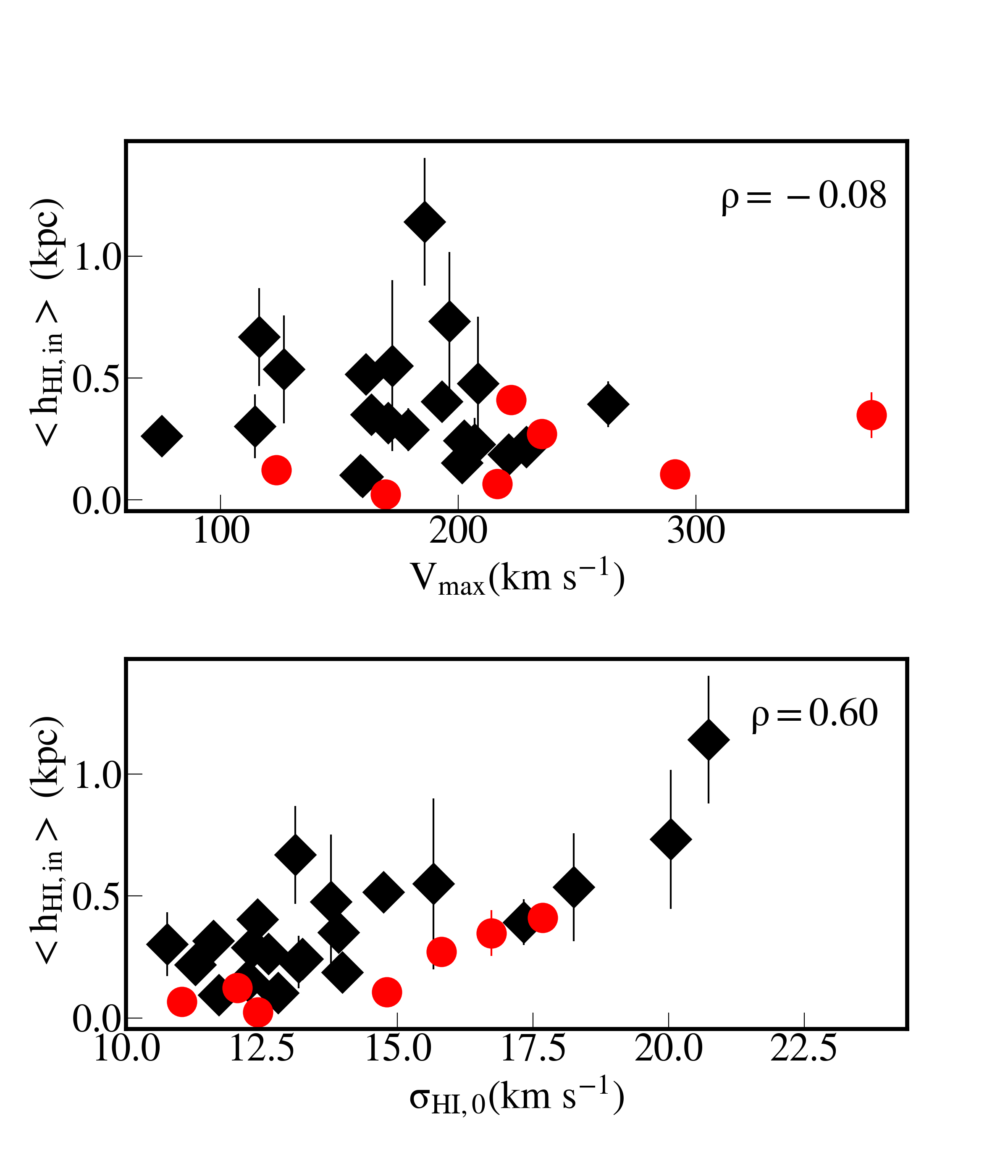
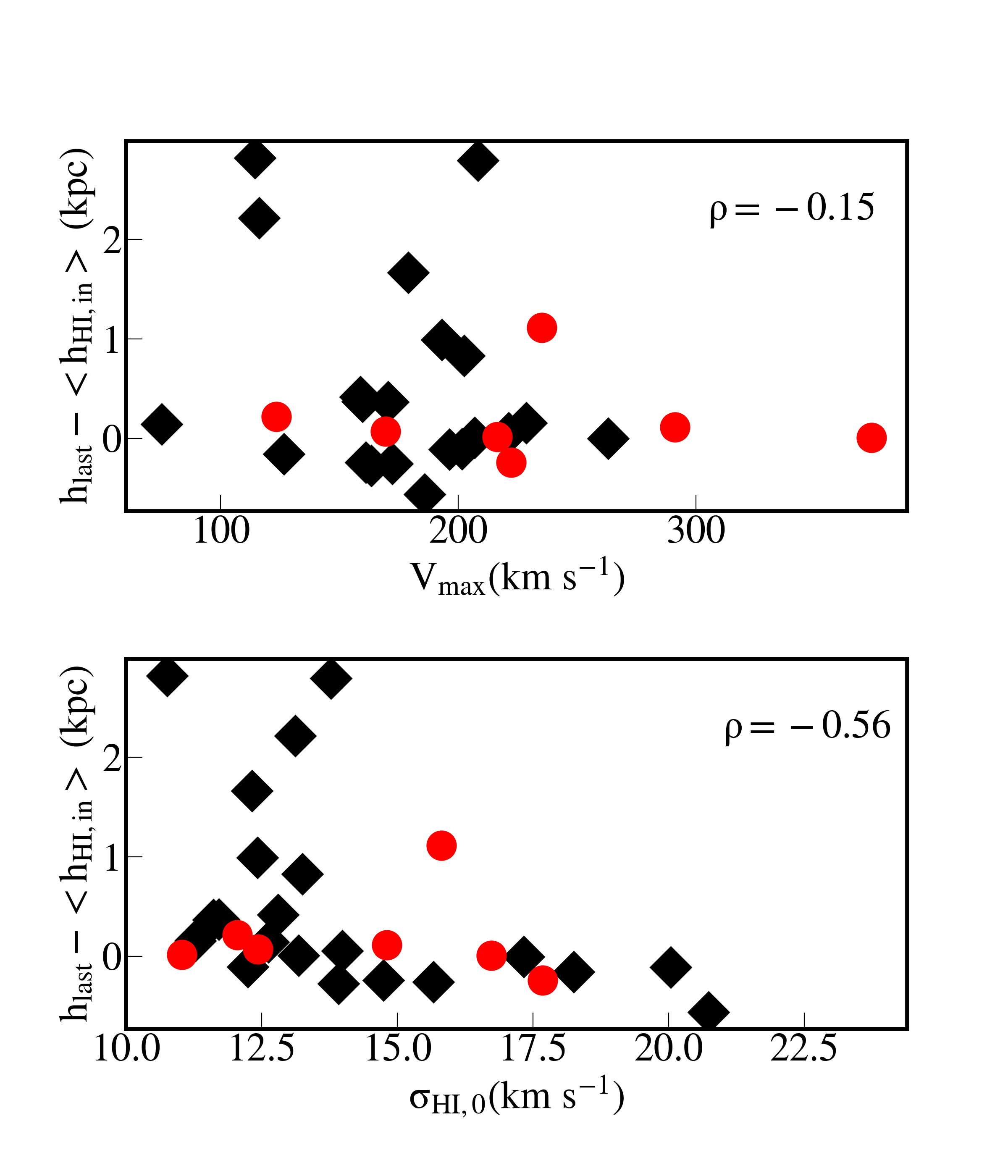
The average Hi scale height within the optical disk are summarized in Table 1. The central velocity dispersion and the circular velocity Vmax are plotted against the average Hi scale height inside the optical disk on the left panels of Figure 11 and the flaring amplitude hlast - <hHI,in> on the right panels. The bottom panels of this figure show clear trend with velocity dispersion. Galaxies with larger central Hi velocity dispersion are thicker on average and do not exhibit disk flaring.
III.4 Correlations with galaxy global properties
This section discusses relationships between the estimated Hi scale height inside the optical disk with global optical and Hi properties. We found no correlation between the R-band concentration index (R90/R50) and the Hi scale height as shown on the left panel of Figure 12 with a Pearson correlation coefficient of -0.04 and a p-value of 0.95. We also did not find any correlation between the Hi scale height and the Hi concentration index (R90/R50)HI which is the ratio between the radius that contain 90% and 50% of the Hi fluxes ( 0.04 and p-value 0.94) and the ratio between the radius of the Hi and optical disk ( 0.03 and p-value 0.97). These results imply that for the Bluedisk galaxies, there are no relation between the vertical extend of the Hi and the central concentration of the stars and gas.
We also explore the relation between the Hi disk thickness with the atomic gas fraction. Figure 13 plots the ratio between the Hi and stellar mass as a function of the Hi scale height. The bottom panel of this figure shows that the Hi scale height is strongly correlated with the Hi fraction estimated within the optical disk with a Pearson correlation of 0.77 and a p-value 10-6. We further added galaxies form the THINGS and VIVA Hi surveys to the relation and used the atomic gas fraction instead of Hi fraction. The bottom panel of Figure 14 shows a strong correlation between the atomic gas fraction inside the optical disk with the Hi disk thickness. We derive the following scaling relation between the Hi disk scale height and the atomic gas fraction measured inside the optical disk:
| (10) |
where the atomic gas fraction inside the optical disk is given by
| (11) |
The 1- scatter is smaller 0.22 dex if is used compared to 0.38 dex if is used instead. The relation between the HI scale height and atomic gas fraction can be expressed as
| (12) |
where and are constants.
III.5 The Hi scale height-atomic gas fraction relation
We checked if the relation between the Hi scale height and the atomic gas fraction relation measured inside the optical disk is produced to a specific sample. We derive the relation using different combination of the sample using the total atomic gas fraction in Figure 15. The fitting results are summarized in Table 2. We found no correlation between scale height and the total atomic gas fraction if only the BLUEDISK Hi rich galaxies are used in the fit with a p-value of 0.031. The fit improves when control galaxies are also added to the fit but the p-value of 0.002 still suggest no correlation. The scatter also increases by 0.1 dex. A correlation is found when both the THINGS and VIVA are also added to the fit. However, the relation becomes more flat with a slope of 0.6 compared to 1.1 when BLUEDISK galaxies alone are used. This change of slope is mainly driven by the VIVA galaxies that have lower Hi fraction but similar scale heights with the THINGS and BLUEDISK galaxies. On the other hand, a clear correlation is found when the atomic gas fraction inside the optical disk is used. The fitting results are shown in Figure 16 and summarized in Table 3 for the fit using the atomic gas fraction inside the optical disk. The slope of the relation also does not change significantly when adding more galaxies and the scatter is smaller compared to slope obtained when the total atomic gas fraction is used. Upcoming survey such as WALLABY will provide us with a large enough sample that span a wide range of Hi fraction and will give us a clear picture on the Hi scale height-atomic gas fraction relation.
III.6 Relation with star formation rates and molecular gas content
In this section we explore the correlation between Hi scale height with the molecular gas content and SFR. In Figure 17, the star formation rates, star formation rates per unit gas (atomic and molecular) and specific star formation rates are plotted as a function of the HI scale height inside the optical disk. This figure shows that the scale height is correlated with the specific star formation rate and the star formation rate per molecular gas mass with a p-value smaller than 0.001. No correlation was found between the Hi thickness and the star formation rate nor the star formation rate per Hi mass. In Figure 18, the molecular to Hi ratio inside the optical disk (top) and the total molecular to Hi ratio (bottom) are plotted as a function of the Hi scale height. This figure shows that the Hi scale height is more correlated with the Hi to the molecular inside the optical disk with correlation coefficient of 0.58 and a p-value of < 0.001 and not with the total molecular to Hi ratio. Note that theoretically, mid-plane pressure is a key factor in both setting the Hi thickness, and the conversion of Hi to the molecular (Ostriker et al. 2010; Blitz & Rosolowsky 2006). The role of mid-plane pressure in setting H2 to Hi conversion has been confirmed by Leroy et al. 2008.
IV Summary
We used an empirical relation from Wilson et al. 2019 to estimated the average Hi scale-height of spiral galaxies selected from BLUEDISK (Wang et al. 2013), THINGS (Walter et al. 2008) and VIVA (Chung et al. 2009) Hi surveys. We investigated correlations between the HI scale height with other optical and HI global properties.
Our main results are as follow:
- •
The HI-rich galaxies from BLUEDISK have similar Hi disk thickness inside the optical disk on average (0.41 0.29 kpc) to the control galaxies (0.29 0.14 kpc), THINGS (0.68 0.58 kpc) and VIVA (0.31 0.25 kpc) galaxies.
- •
The Hi scale height radial profiles can be divided into three categories. The first category consist of galaxies where the Hi disk thickness increases with radius, the second category have a Hi scale height that is constant with radius and the third category have complex scale height radial profiles. The complexity may reflect a mixture of effects from gas inflow, the resulted radial distribution of gas surface density , stellar feedback and environmental effects.
- •
The average Hi scale height within the optical disk is correlated with the atomic gas fraction. Such correlations would be useful when estimating the Hi disk thickness of large sample of galaxies.
- •
The average scale height within the optical disk is also correlated with the central Hi velocity dispersion. However, a larger sample is needed before further interpretation.
- •
The relation between and the Hi scale height confirm the role of gas disk thickness on star formation efficiency which have been previously reported ( e.g. Leroy et al. 2008).
Measuring the gas disk thickness is a challenging task and direct measurements are only available for handful of edge-on galaxies. A scaling relation is therefore crucial and will allow us to estimate the vertical extend of Hi in large sample of galaxies. The WALLABY survey will observe 500000 galaxies but most of these will be unresolved. Single dish radio telescope such as FAST will detect a large number of galaxies in HI. These upcoming survey will provide HI masses for a significant number of galaxies. We can therefore explore statistically the effect of the vertical extend of HI on star formation efficiency in nearby disk galaxies.
Dedicated survey of edge-on galaxies will increase the number of galaxies with measured scale height and will help us to better understand the vertical distribution of Hi. This will also allow us to test different theories of vertical equilibrium.
References
- Abramova & Zasov (2008) Abramova, O. V., & Zasov, A. V. 2008, Astronomy Reports, 52, 257
- Bacchini et al. (2019a) Bacchini, C., Fraternali, F., Pezzulli, G., et al. 2019, A&A, 632, A127
- Bacchini et al. (2019b) Bacchini, C., Fraternali, F., Iorio, G., et al. 2019, A&A, 622, A64
- Banerjee et al. (2011) Banerjee, A., Jog, C. J., Brinks, E., et al. 2011, MNRAS, 415, 687
- Bekiaris et al. (2016) Bekiaris, G., Glazebrook, K., Fluke, C. J., et al. 2016, MNRAS, 455, 754
- Begeman (1989) Begeman, K. G. 1989, A&A, 223, 47
- Bosma (1981) Bosma, A. 1981, AJ, 86, 1825
- Blitz & Rosolowsky (2006) Blitz, L. & Rosolowsky, E. 2006, ApJ, 650, 933. doi:10.1086/505417
- Catinella et al. (2012) Catinella, B., Schiminovich, D., Kauffmann, G., et al. 2012, A&A, 544, A65
- Chung et al. (2009) Chung, A., van Gorkom, J. H., Kenney, J. D. P., et al. 2009, AJ, 138, 1741
- Cormier et al. (2016) Cormier, D., Bigiel, F., Wang, J., et al. 2016, MNRAS, 463, 1724. doi:10.1093/mnras/stw2097
- Courteau (1997) Courteau, S. 1997, AJ, 114, 2402
- Chyży et al. (2017) Chyży, K. T., Sridhar, S. S., & Jurusik, W. 2017, A&A, 603, A121. doi:10.1051/0004-6361/201730690
- de Avillez & Breitschwerdt (2005) de Avillez, M. A., & Breitschwerdt, D. 2005, A&A, 436, 585
- de Blok et al. (2008) de Blok, W. J. G., Walter, F., Brinks, E., et al. 2008, AJ, 136, 2648
- Di Teodoro & Fraternali (2015) Di Teodoro, E. M., & Fraternali, F. 2015, MNRAS, 451, 3021
- Dutta et al. (2009) Dutta, P., Begum, A., Bharadwaj, S., et al. 2009, MNRAS, 397, L60
- Hoffmann & Romeo (2012) Hoffmann, V. & Romeo, A. B. 2012, MNRAS, 425, 1511
- Sancisi & Allen (1979) Sancisi, R., & Allen, R. J. 1979, A&A, 74, 73
- Silich & Tenorio-Tagle (1998) Silich, S. A., & Tenorio-Tagle, G. 1998, MNRAS, 299, 249
- Spitzer (1942) Spitzer L., 1942, ApJ, 95, 329
- Girichidis et al. (2016) Girichidis, P., Naab, T., Walch, S., et al. 2016, ApJ, 816, L19
- Schmidt (1959) Schmidt, M. 1959, ApJ, 129, 243
- Swaters et al. (1997) Swaters, R. A., Sancisi, R., & van der Hulst, J. M. 1997, ApJ, 491, 140
- Tamburro et al. (2009) Tamburro, D., Rix, H.-W., Leroy, A. K., et al. 2009, AJ, 137, 4424
- Tabatabaei et al. (2013a) Tabatabaei, F. S., Berkhuijsen, E. M., Frick, P., et al. 2013, A&A, 557, A129. doi:10.1051/0004-6361/201218909
- Tabatabaei et al. (2013b) Tabatabaei, F. S., Schinnerer, E., Murphy, E. J., et al. 2013, A&A, 552, A19. doi:10.1051/0004-6361/201220249
- Józsa et al. (2007) Józsa, G. I. G., Kenn, F., Klein, U., et al. 2007, A&A, 468, 731
- Iorio (2018) Iorio,G. 2018, PhD thesis, University of Bologna
- Olling (1995) Olling, R. P. 1995, AJ, 110, 591
- Olling (1996) Olling, R. P. 1996, AJ, 112, 457
- Ostriker et al. (2010) Ostriker, E. C., McKee, C. F., & Leroy, A. K. 2010, ApJ, 721, 975. doi:10.1088/0004-637X/721/2/975
- Parker (1966) Parker, E. N. 1966, ApJ, 145, 811. doi:10.1086/148828
- Leroy et al. (2008) Leroy, A. K., Walter, F., Brinks, E., et al. 2008, AJ, 136, 2782. doi:10.1088/0004-6256/136/6/2782
- Mogotsi et al. (2016) Mogotsi, K. M., de Blok, W. J. G., Caldú-Primo, A., et al. 2016, AJ, 151, 15
- Read et al. (2016) Read, J. I., Iorio, G., Agertz, O., et al. 2016, MNRAS, 462, 3628
- Romeo et al. (2010) Romeo, A. B., Burkert, A., & Agertz, O. 2010, MNRAS, 407, 1223
- Romeo & Agertz (2014) Romeo, A. B. & Agertz, O. 2014, MNRAS, 442, 1230
- Hill et al. (2018) Hill, A. S., Mac Low, M.-M., Gatto, A., et al. 2018, ApJ, 862, 55
- Iorio et al. (2017) Iorio, G., Fraternali, F., Nipoti, C., et al. 2017, MNRAS, 466, 4159
- Padoan et al. (2001) Padoan, P., Kim, S., Goodman, A., et al. 2001, ApJ, 555, L33
- van der Kruit (1981) van der Kruit, P. C. 1981, A&A, 99, 298
- Kennicutt (1998) Kennicutt, R. C. 1998, ARA&A, 36, 189
- Krumholz et al. (2018) Krumholz, M. R., Burkhart, B., Forbes, J. C., et al. 2018, MNRAS, 477, 2716. doi:10.1093/mnras/sty852
- Kim & Ostriker (2015) Kim, C.-G. & Ostriker, E. C. 2015, ApJ, 802, 99. doi:10.1088/0004-637X/802/2/99
- Van Eck et al. (2015) Van Eck, C. L., Brown, J. C., Shukurov, A., et al. 2015, ApJ, 799, 35. doi:10.1088/0004-637X/799/1/35
- Wang et al. (2013) Wang, J., Kauffmann, G., Józsa, G. I. G., et al. 2013, MNRAS, 433, 270
- Wang et al. (2014) Wang, J., Fu, J., Aumer, M., et al. 2014, MNRAS, 441, 2159
- Wang et al. (2020) Wang, J., Catinella, B., Saintonge, A., et al. 2020, ApJ, 890, 63. doi:10.3847/1538-4357/ab68dd
- Walter et al. (2008) Walter, F., Brinks, E., de Blok, W. J. G., et al. 2008, AJ, 136, 2563
- Wilson et al. (2019) Wilson, C. D., Elmegreen, B. G., Bemis, A., et al. 2019, ApJ, 882, 5
Appendix A Hi scale heights of the remaining BLUEDISK galaxies


