跳到论文正文
W Papers独立论文阅读器 arXiv:2105.10668 论文正文 计算阅读时间 · 0%
引用这篇论文根据当前论文元数据生成,正式投稿前建议核对。


License: arXiv.org perpetual non-exclusive license
arXiv:2105.10668v2 [cs.CR] 18 Nov 2021

Runtime Enforcement of Programmable Logic ControllersJournal: TOPSCCS: Security and privacy Formal security modelsCCS: Security and privacy Cyber-physical systems security

Ruggero Lanotte OrcID: 0000-0002-3335-234X Affiliation: Università degli Studi dell’Insubria , Dipartimento di Scienze Umane e dell’Innovazione per il Territorio, via Sant’Abbondio 12 , Como , 22100 , Italy email: ruggero.lanotte@uninsubria.it , Massimo Merro OrcID: 0000-0002-1712-7492 Affiliation: Università degli Studi di Verona , Dipartimento di Informatica, strada Le Grazie 15 , Verona , 37134 , Italy email: massimo.merro@univr.it and Andrei Munteanu Affiliation: Università degli Studi di Verona , Dipartimento di Informatica, strada Le Grazie 15 , Verona , 37134 , Italy email: andrei.munteanu@univr.it
Abstract.

With the advent of Industry 4.0, industrial facilities and critical infrastructures are transforming into an ecosystem of heterogeneous physical and cyber components, such as programmable logic controllers, increasingly interconnected and therefore exposed to cyber-physical attacks, i.e., security breaches in cyberspace that may adversely affect the physical processes underlying industrial control systems.

In this paper, we propose a formal approach based on runtime enforcement to ensure specification compliance in networks of controllers, possibly compromised by colluding malware that may tamper with actuator commands, sensor readings, and inter-controller communications. Our approach relies on an ad-hoc sub-class of Ligatti et al.’s edit automata to enforce controllers represented in Hennessy and Regan’s Timed Process Language. We define a synthesis algorithm that, given an alphabet 𝒫\mathcal{P} of observable actions and a timed correctness property ee, returns a monitor that enforces the property ee during the execution of any (potentially corrupted) controller with alphabet 𝒫\mathcal{P}, and complying with the property ee. Our monitors correct and suppress incorrect actions coming from corrupted controllers and emit actions in full autonomy when the controller under scrutiny is not able to do so in a correct manner. Besides classical requirements, such as transparency and soundness, the proposed enforcement enjoys deadlock- and diverge-freedom of monitored controllers, together with scalability when dealing with networks of controllers. Finally, we test the proposed enforcement mechanism on a non-trivial case study, taken from the context of industrial water treatment systems, in which the controllers are injected with different malware with different malicious goals.

Keywords: 
Runtime enforcement, control systems security, PLC malware

1. Introduction

Industrial Control Systems (ICSs) are physical and engineered systems whose operations are monitored, coordinated, controlled, and integrated by a computing and communication core (Rajkumar et al. 2010). They represent the backbone of Critical Infrastructures for safety-critical applications such as electric power distribution, nuclear power production, and water supply.

The growing connectivity and integration in Industry 4.0 has triggered a dramatic increase in the number of cyber-physical attacks (Huang et al. 2009) targeting ICSs, i.e., security breaches in cyberspace that adversely affect the physical processes. Some notorious examples are: (i) the Stuxnet worm, which reprogrammed Siemens PLCs of nuclear centrifuges in the nuclear facility of Natanz in Iran (Kushner 2013); (ii) the CRASHOVERRIDE attack on the Ukrainian power grid, otherwise known as Industroyer (Slowik 2018); (iii) the recent TRITON/TRISIS malware that targeted a petrochemical plant in Saudi Arabia (Di Pinto et al. 2018).

One of the key components of ICSs are Programmable Logic Controllers, better known as PLCs. They control mission-critical electrical hardware such as pumps or centrifuges, effectively serving as a bridge between the cyber and the physical worlds. PLCs have an ad-hoc architecture to execute simple repeating processes known as scan cycles (IEC 61131-3 (61131-3 2003)). Each scan cycle consists of three phases: (i) reading of sensor measurements of the physical process; (ii) execution of the controller code to compute how the physical process should evolve; (iii) transmission of commands to the actuator devices to govern the physical process as desired.

Due to their sensitive role in controlling industrial processes, successful exploitation of PLCs can have severe consequences on ICSs. In fact, although modern controllers provide security mechanisms to allow only legitimate firmware to be uploaded, the running code can be typically altered by anyone with network or USB access to the controllers (see Figure 1). Published scan data shows how thousands of PLCs are directly accessible from the Internet to improve efficiency (Radvanovsky 2013). Thus, despite their responsibility, controllers are vulnerable to several kinds of attacks, including PLC-Blaster worm (Spenneberg et al. 2016), Ladder Logic Bombs (Govil et al. 2018), and PLC PIN Control attacks (Abbasi and Hashemi 2016).

Refer to caption
Figure 1. A network of compromised PLCs: yiy_{i} denote genuine sensor measurements, yiay_{i}^{\mathrm{a}} are corrupted sensor measurements, uiau_{i}^{\mathrm{a}} corrupted actuator commands, and ciac_{i}^{\mathrm{a}} denote corrupted inter-controller communications.

Extra trusted hardware components have been proposed to enhance the security of PLC architectures (McLaughlin 2013; Mohan et al. 2013). For instance, McLaughlin (McLaughlin 2013) proposed a policy-based enforcement mechanism to mediate the actuator commands transmitted by the PLC to the physical plant. Mohan et al. (Mohan et al. 2013) introduced a different architecture, in which every PLC runs under the scrutiny of a monitor which looks for deviations with respect to safe behaviours. Both architectures have been validated by means of simulation-based techniques. However, as far as we know, formal methodologies have been rarely used to model and formally verify security-oriented architectures for ICSs.

Runtime enforcement (Schneider 2000; Ligatti et al. 2005; Falcone et al. 2011) is a formal verification/validation technique aiming at correcting possibly-incorrect executions of a system-under-scrutiny (SuS). It employs a kind of monitor (Francalanza 2021) that acts as a proxy between the SuS and the environment interacting with it. At runtime, the monitor transforms any incorrect executions exhibited by the SuS into correct ones by either replacing, suppressing or inserting observable actions on behalf of the system. The effectiveness of the enforcement depends on the achievement of the two following general principles (Schneider 2000; Ligatti et al. 2005):

  • •

    transparency, i.e., the enforcement must not alter correct executions of the SuS;

  • •

    soundness, i.e., incorrect executions of the SuS must be prevented.

In this paper, we propose a formal approach based on runtime enforcement to ensure specification compliance in networks of controllers possibly compromised by colluding malware that may tamper with actuator commands, sensor readings, and inter-controller communications. combined with automatic recovery mechanisms.

Our goal is to enforce potentially corrupted controllers using secure proxies based on a sub-class of Ligatti et al.’s edit automata (Ligatti et al. 2005). These automata will be synthesised from enforceable timed correctness properties to form networks of monitored controllers, as in Figure 2. The proposed enforcement will enjoy both transparency and soundness together with the following features:

  • •

    determinism preservation, i.e., the enforcement should not introduce nondeterminism;

  • •

    deadlock-freedom, i.e., the enforcement should not introduce deadlocks;

  • •

    divergence-freedom, i.e., the enforcement should not introduce divergencies;

  • •

    mitigation of incorrect/malicious activities;

  • •

    scalability, i.e., the enforcement mechanism should scale to networks of controllers.

Obviously, when a controller is compromised, these objectives can be achieved only with the introduction of a physically independent secure proxy, as advocated by McLaughlin and Mohan et al. (McLaughlin 2013; Mohan et al. 2013), which does not have any Internet or USB access, and which is connected with the monitored controller via secure channels. This may seem like we just moved the problem over to securing the proxy. However, this is not the case because the proxy only needs to enforce a timed correctness property of the system, while the controller does the whole job of controlling the physical process relying on potentially dangerous communications via the Internet or the USB ports. Thus, any upgrade of the control system will be made to the controller and not to the secure proxy. Of course, by no means runtime reconfigurations of the secure proxy should be allowed as its enforcing should be based on the physics of the plant itself and not on the controller code.
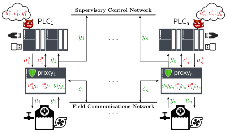
Refer to caption
Figure 2. A network of monitored controllers.
Contribution

Fist of all, we define the attacker model and the attacker objectives in an enforced ICS architecture such as that depicted in Figure 2. Then, we introduce a formal language to specify controller programs. For this very purpose, we resort to process calculi, a successful and widespread formal approach in concurrency theory for representing complex systems, such as mobile systems (Cardelli and Gordon 2000) and cyber-physical systems (Lanotte et al. 2020b), and used in many areas, including verification of security protocols (Abadi et al. 2018; Abadi and Gordon 1997) and security analysis of cyber-physical attacks (Lanotte et al. 2020c). Thus, we define a simple timed process calculus, based on Hennessy and Regan’s Timed Process Language (TPL) (Hennessy and Regan 1995), for specifying controllers, finite-state enforcers, and networks of communicating monitored controllers.

Then, we define a simple description language to express timed correctness properties that should hold for a (possibly unbounded) number of scan cycles of the monitored controller. This will allow us to abstract over controllers implementations, focusing on general properties which may even be shared by completely different controllers. In this regard, we might resort to one of the several logics existing in the literature for monitoring timed concurrent systems, and in particular cyber-physical systems (see, e.g., (Bartocci et al. 2018; Frehse et al. 2018)). However, the peculiar iterative behaviour of controllers convinced us to adopt the sub-class of regular expressions that can be recognised by finite automata whose cycles always contain at least one final state; this is the largest class of regular properties that can be enforced by finite-state Ligatti et at.’s edit automata (see Beauquier et al.’s work (Beauquier et al. 2013)). In Section 5, we express a wide class of correctness properties for controllers in terms of (our) regular properties.

After defining a formal language to describe controller properties, we provide a synthesis function ⟨|−|⟩𝒫{\langle\!|\!{-}\!|\!\rangle^{\mathcal{P}}} that, given an alphabet 𝒫\mathcal{P} of observable actions (sensor readings, actuator commands, and inter-controller communications) and a deterministic regular property ee combining events of 𝒫\mathcal{P}, returns an edit automaton ⟨|e|⟩𝒫{\langle\!|\!{e}\!|\!\rangle^{\mathcal{P}}}\!. The resulting enforcement mechanism will ensure the required features mentioned before: transparency, soundness, determinism preservation, deadlock-freedom, divergence-freedom, mitigation and scalability. Then, we propose a non-trivial case study, taken from the context of industrial water treatment systems, and implemented as follows: (i) the physical plant is simulated in Simulink (MATLAB 2018); (ii) the open source PLCs are implemented in OpenPLC (Alves et al. 2014) and executed on Raspberry Pi; (iii) the enforcers run on connected FPGAs. In this setting, we test our enforcement mechanism when injecting the PLCs with 55 different malware, with different goals.

Outline

Section 2 describes the attacker model and the attacker objectives. Section 3 gives a formal language for monitored controllers. Section 4 defines the case study. Section 5 provides a language of regular properties to express controller behaviours; it also contains a taxonomy of properties expressible in the language. Section 6 contains the algorithm to synthesise monitors from regular properties, together with the main results. Section 7 discusses the implementation of the case study when exposed to five different attacks. Section 8 is devoted to related work. Section 9 draws conclusions and discusses future work. Technical proofs can be found in the appendix.

2. Attacker model and attacker objectives

In the following sections, we will propose an enforcement-based architecture for ICSs (as those depicted in Figure 2) to counter attacks complying with the following attacker model:

  • •

    malware injected in one or more PLCs may forge/drop actuator commands, modify sensor readings coming from the plant, forge/drop inter-controller communications;

  • •

    malware injected in different PLCs of the same field communications network may collaborate/communicate with each other to achieve common objectives;

  • •

    the attacker runtime behaviour may vary as it may depend on the received sensor signals and the communications with other PLCs;

  • •

    malicious alterations of sensor signals at network level, or within the sensor devices, are not allowed (they are out of the scope of this paper);

  • •

    scan cycles must be completed within a specific time, called maximum cycle limit, which depends on the controlled physical process; if this time limit is violated then the controller stops and throws an exception (Spenneberg et al. 2016); we assume that the injected malware never violates the maximum cycle limit because not interested in causing the immediate shutdown of a PLC;

  • •

    the enforcers added in the architecture are physically independent secure proxies with no Internet or USB access, and connected with the controller via secure channels; as a consequence, the measurements transmitted to the supervisory control network will not be corrupted;

  • •

    runtime reconfigurations of secure proxies are not allowed.

Thus, in general, the attacker objectives can be resumed in alteration/forgery of PLC actuator commands and/or communication messages between PLCs to eventually affect the evolution of the controlled physical processes, and/or transmit fake signals to the supervisory control network.

3. A Formal language for monitored controllers

In this section, we introduce the Timed Calculus of Monitored Controllers, called TCMC, as an abstract formal language to express networks of controllers integrated with edit automata sitting on the network interface of each controller to monitor/correct their interactions with the rest of the system. Basically, TCMC extends Hennessy and Regan’s Timed Process Language (TPL) (Hennessy and Regan 1995) with monitoring edit automata. Like TPL time proceeds in discrete time slots separated by 𝗍𝗂𝖼𝗄{\scriptstyle\mathsf{tick}}-actions.

Let us start with some preliminary notation. We use s,sk∈𝖲𝖾𝗇𝗌s,s_{k}\in\mathsf{Sens} to name sensor signals; a,ak∈𝖠𝖼𝗍a,a_{k}\in\mathsf{Act} to indicate actuator commands; c,ck∈𝖢𝗁𝗇c,c_{k}\in\mathsf{Chn} for channels; z,zkz,z_{k} for generic names.

Controllers

In our setting, controllers are nondeterministic sequential timed processes evolving through three main phases: sensing of sensor signals, communication with other controllers, and actuation. For convenience, we use five different syntactic categories to distinguish the five main states of a controller: ℂ​𝕥​𝕣​𝕝\mathbbm{Ctrl} for initial states, 𝕊​𝕝​𝕖​𝕖​𝕡\mathbbm{Sleep} for sleeping states, 𝕊​𝕖​𝕟​𝕤\mathbbm{Sens} for sensing states, ℂ​𝕠​𝕞\mathbbm{Com} for communication states, and 𝔸​𝕔​𝕥\mathbbm{Act} for actuation states. In its initial state, a controller is a recursive process waiting for signal stabilisation in order to start the sensing phase:

ℂ​𝕥​𝕣​𝕝∋P:⁣:=X𝕊​𝕝​𝕖​𝕖​𝕡∋W:⁣:=𝗍𝗂𝖼𝗄.W|S\begin{array}[]{rcl}\mathbbm{Ctrl}\ni P&\>\;::=&X\\ \mathbbm{Sleep}\ni W&\>\;::=&{\scriptstyle\mathsf{tick}}.W\quad\big|\quad S\end{array}

The main process describing a controller consists of some recursive process defined via equations of the form X=𝗍𝗂𝖼𝗄.WX={\scriptstyle\mathsf{tick}}.W, with W∈𝕊​𝕝​𝕖​𝕖​𝕡W\in\mathbbm{Sleep}; here, XX is a process variable that may occur (free) in WW. For convenience, our controllers always have at least one initial timed action 𝗍𝗂𝖼𝗄{\scriptstyle\mathsf{tick}} to ensure time-guarded recursion, thus avoiding undesired zeno behaviours (Heymann et al. 2005): the number of untimed actions between two 𝗍𝗂𝖼𝗄{\scriptstyle\mathsf{tick}}-actions is always finite. Then, after a determined sleeping period, when sensor signals get stable, the sensing phase can start.

During the sensing phase, the controller waits for a finite number of admissible sensor signals. If none of those signals arrives in the current time slot then the controller will timeout moving to the following time slot (we adopt the TPL construct ⌊⋅⌋⋅\lfloor\cdot\rfloor\cdot for timeout). The syntax is the following:

𝕊​𝕖​𝕟​𝕤∋S:⁣:=⌊∑i∈Isi.Si⌋S|C\begin{array}[]{rcl}\mathbbm{Sens}\ni S&\>\;::=&\lfloor\sum_{i\in I}s_{i}.S_{i}\rfloor S\quad\big|\quad C\end{array}

where ∑i∈Isi.Si\sum_{i\in I}s_{i}.S_{i} denotes the standard construct for nondeterministic choice. Once the sensing phase is concluded, the controller starts its calculations that may depend on communications with other controllers governing different physical processes. Controllers communicate with each other for mainly two reasons: either to receive notice about the state of other physical sub-processes or to require an actuation on a physical process which is out of their control. As in TPL, we adopt a channel-based handshake point-to-point communication paradigm. Note that, in order to avoid starvation, communication is always under timeout. The syntax for the communication phase is:

ℂ​𝕠​𝕞​𝕞∋C:⁣:=⌊∑i∈Ici.Ci⌋C|⌊c¯.C⌋C|A\begin{array}[]{rcl}\mathbbm{Comm}\ni C&\>\;::=&\lfloor\sum_{i\in I}c_{i}.C_{i}\rfloor C\quad\big|\quad\lfloor\overline{c}.C\rfloor C\quad\big|\quad A\end{array}

In the actuation phase a controller eventually transmits a finite sequence of commands to actuators, and then, it emits a fictitious system signal 𝖾𝗇𝖽{\scriptstyle\mathsf{end}} to denote the end of the scan cycle. After that, the whole scan cycle can restart. Formally,

𝔸​𝕔​𝕥∋A:⁣:=a¯.A|𝖾𝗇𝖽.X\begin{array}[]{rcl}\mathbbm{Act}\ni A&\>\;::=&\overline{a}.A\quad\big|\quad{\scriptstyle\mathsf{end}}.X\end{array}
Remark 1 (Scan cycle duration and maximum cycle limit).

The scan cycle of a PLC must be completed within a specific time, called maximum cycle limit, which depends on the controlled physical process; if this time limit is violated the the controller stops and throws an exception (Spenneberg et al. 2016). Thus, the signal 𝖾𝗇𝖽{\scriptstyle\mathsf{end}} must occur well before the maximum cycle limit of the controller. We actually work under the assumption that our controllers successfully complete their scan cycle in less than half of the maximum cycle limit. The reasons for this assumption will be clarified in Remark 4. Please, notice that it is easy to statically derive the maximum duration of a scan cycle expressed in our calculus by simply counting the maximum number of 𝗍𝗂𝖼𝗄{\scriptstyle\mathsf{tick}}-prefixes occurring between two subsequent 𝖾𝗇𝖽{\scriptstyle\mathsf{end}}-prefixes.

(Sleep)​−𝗍𝗂𝖼𝗄.W-𝗍𝗂𝖼𝗄⁣→W(Rec)​X=𝗍𝗂𝖼𝗄.WX-𝗍𝗂𝖼𝗄⁣→W(ReadS)​j∈I⌊∑i∈Isi.Si⌋S-sj⁣→Sj(TimeoutS)​−⌊∑i∈Isi.Si⌋S-𝗍𝗂𝖼𝗄⁣→S(InC)​j∈I⌊∑i∈Ici.Ci⌋C-cj⁣→Cj(TimeoutInC)​−⌊∑i∈Ici.Ci⌋C-𝗍𝗂𝖼𝗄⁣→C(OutC)​−⌊c¯.C⌋C′-c¯⁣→C(TimeoutOutC)​−⌊c¯.C⌋C′-𝗍𝗂𝖼𝗄⁣→C′(WriteA)​−a¯.A-a¯⁣→A(End)​−𝖾𝗇𝖽.X-𝖾𝗇𝖽⁣→X\begin{array}[]{l@{\hspace*{8mm}}l}{\mbox{\small(Sleep)}}\>\;\begin{array}[]{c}-\\[2.0pt] \hline\cr{{\scriptstyle\mathsf{tick}}.W\mathrel{\;\raisebox{0.0pt}{$\stackrel{{\scriptstyle\,{\scriptstyle\mathsf{tick}}}}{{\makebox[16.71004pt]{\rule{0.0pt}{3.87498pt}\mbox{}\leaders{\hbox{$\mkern-2.6mu\relbar\mkern-2.6mu$}}{\hfill}\mbox{}}}}$}\hskip-8.52495pt\rightarrow}W}\end{array}\hfil\hskip 22.76219pt&{\mbox{\small(Rec)}}\>\;\begin{array}[]{c}X={\scriptstyle\mathsf{tick}}.W\\[2.0pt] \hline\cr{X\mathrel{\;\raisebox{0.0pt}{$\stackrel{{\scriptstyle\,{\scriptstyle\mathsf{tick}}}}{{\makebox[16.71004pt]{\rule{0.0pt}{3.87498pt}\mbox{}\leaders{\hbox{$\mkern-2.6mu\relbar\mkern-2.6mu$}}{\hfill}\mbox{}}}}$}\hskip-8.52495pt\rightarrow}W}\end{array}\\[10.0pt] {\mbox{\small(ReadS)}}\>\;\begin{array}[]{c}j\in I\\[2.0pt] \hline\cr\lfloor\sum_{i\in I}s_{i}.S_{i}\rfloor S\mathrel{\;\raisebox{0.0pt}{$\stackrel{{\scriptstyle\,s_{j}}}{{\makebox[13.343pt]{\rule{0.0pt}{3.87498pt}\mbox{}\leaders{\hbox{$\mkern-2.6mu\relbar\mkern-2.6mu$}}{\hfill}\mbox{}}}}$}\hskip-8.52495pt\rightarrow}{S_{j}}\end{array}\hfil\hskip 22.76219pt&{\mbox{\small(TimeoutS)}}\>\;\begin{array}[]{c}-\\[2.0pt] \hline\cr\lfloor\sum_{i\in I}s_{i}.S_{i}\rfloor S\mathrel{\;\raisebox{0.0pt}{$\stackrel{{\scriptstyle\,{\scriptstyle\mathsf{tick}}}}{{\makebox[16.71004pt]{\rule{0.0pt}{3.87498pt}\mbox{}\leaders{\hbox{$\mkern-2.6mu\relbar\mkern-2.6mu$}}{\hfill}\mbox{}}}}$}\hskip-8.52495pt\rightarrow}{S}\end{array}\\[10.0pt] {\mbox{\small(InC)}}\>\;\begin{array}[]{c}j\in I\\[2.0pt] \hline\cr\lfloor\sum_{i\in I}c_{i}.C_{i}\rfloor C\mathrel{\;\raisebox{0.0pt}{$\stackrel{{\scriptstyle\,c_{j}}}{{\makebox[13.18332pt]{\rule{0.0pt}{3.87498pt}\mbox{}\leaders{\hbox{$\mkern-2.6mu\relbar\mkern-2.6mu$}}{\hfill}\mbox{}}}}$}\hskip-8.52495pt\rightarrow}{C_{j}}\end{array}\par\hfil\hskip 22.76219pt&{\mbox{\small(TimeoutInC)}}\>\;\begin{array}[]{c}-\\[2.0pt] \hline\cr\lfloor\sum_{i\in I}c_{i}.C_{i}\rfloor C\mathrel{\;\raisebox{0.0pt}{$\stackrel{{\scriptstyle\,{\scriptstyle\mathsf{tick}}}}{{\makebox[16.71004pt]{\rule{0.0pt}{3.87498pt}\mbox{}\leaders{\hbox{$\mkern-2.6mu\relbar\mkern-2.6mu$}}{\hfill}\mbox{}}}}$}\hskip-8.52495pt\rightarrow}{C}\end{array}\\[10.0pt] {\mbox{\small(OutC)}}\>\;\begin{array}[]{c}-\\[2.0pt] \hline\cr\lfloor\overline{c}.C\rfloor C^{\prime}\mathrel{\;\raisebox{0.0pt}{$\stackrel{{\scriptstyle\,\overline{c}}}{{\makebox[12.05003pt]{\rule{0.0pt}{3.87498pt}\mbox{}\leaders{\hbox{$\mkern-2.6mu\relbar\mkern-2.6mu$}}{\hfill}\mbox{}}}}$}\hskip-8.52495pt\rightarrow}{C}\end{array}\hfil\hskip 22.76219pt&{\mbox{\small(TimeoutOutC)}}\>\;\begin{array}[]{c}-\\[2.0pt] \hline\cr\lfloor\overline{c}.C\rfloor C^{\prime}\mathrel{\;\raisebox{0.0pt}{$\stackrel{{\scriptstyle\,{\scriptstyle\mathsf{tick}}}}{{\makebox[16.71004pt]{\rule{0.0pt}{3.87498pt}\mbox{}\leaders{\hbox{$\mkern-2.6mu\relbar\mkern-2.6mu$}}{\hfill}\mbox{}}}}$}\hskip-8.52495pt\rightarrow}{C^{\prime}}\end{array}\\[10.0pt] {\mbox{\small(WriteA)}}\>\;\begin{array}[]{c}-\\[2.0pt] \hline\cr{\overline{a}.A\mathrel{\;\raisebox{0.0pt}{$\stackrel{{\scriptstyle\,\overline{a}}}{{\makebox[12.05003pt]{\rule{0.0pt}{3.87498pt}\mbox{}\leaders{\hbox{$\mkern-2.6mu\relbar\mkern-2.6mu$}}{\hfill}\mbox{}}}}$}\hskip-8.52495pt\rightarrow}A}\end{array}\hfil\hskip 22.76219pt&{\mbox{\small(End)}}\>\;\begin{array}[]{c}-\\[2.0pt] \hline\cr{{\scriptstyle\mathsf{end}}.X\mathrel{\;\raisebox{0.0pt}{$\stackrel{{\scriptstyle\,{\scriptstyle\mathsf{end}}}}{{\makebox[16.36003pt]{\rule{0.0pt}{3.87498pt}\mbox{}\leaders{\hbox{$\mkern-2.6mu\relbar\mkern-2.6mu$}}{\hfill}\mbox{}}}}$}\hskip-8.52495pt\rightarrow}X}\end{array}\end{array}
Table 1. LTS for controllers.

The operational semantics in Table 1 is along the lines of Hennessy and Regan’s TPL (Hennessy and Regan 1995). In the following, we use the metavariable α\alpha to range over the set of all (observable) controller actions: {s,a¯,c¯,c,𝗍𝗂𝖼𝗄,𝖾𝗇𝖽}\{s,\overline{a},\overline{c},c,{\scriptstyle\mathsf{tick}},{\scriptstyle\mathsf{end}}\}. These actions denote: sensor readings, actuator commands, channel transmissions, channel receptions, passage of time, and end of scan cycles, respectively. Notice that at our level of abstraction we represent only the observable behaviour of PLCs: internal computations are not modelled within PLCs; although, we do have τ\tau-actions to express communications between two PLCs, as the reader will notice in Table 2.

Remark 2 (Attacker model and 𝖾𝗇𝖽{\scriptstyle\mathsf{end}}-signal).

In our abstract representation of PLCs, the 𝖾𝗇𝖽{\scriptstyle\mathsf{end}}-signal is not really part of the (possibly compromised) PLC program but it is rather a system signal denoting the end of a scan cycle. As a consequence, in accordance with our attacker model, we assume that this fictitious signal cannot be dropped or forged by the attacker.

Monitored controllers

The core of our enforcement relies on (timed) finite-state Ligatti et al.’s edit automata (Ligatti et al. 2005), i.e., a particular class of automata specifically designed to allow/suppress/insert actions in a generic system in order to preserve its correct behaviour. The syntax is as follows:

𝔼​𝕕​𝕚​𝕥∋𝖤,𝖥:⁣:=𝗀𝗈|∑i∈Iλi.𝖤i|𝖷{\small\begin{array}[]{rcl}\mathbbm{Edit}\ni\mathsf{E},\mathsf{F}&\>\;::=&\mathsf{go}\hskip 9.24994pt\big|\hskip 9.24994pt\sum_{i\in I}\lambda_{i}.\mathsf{E}_{i}\hskip 9.24994pt\big|\hskip 9.24994pt\mathsf{X}\end{array}}

The special automaton 𝗀𝗈\mathsf{go} will admit any action of the monitored system. The edit automaton ∑i∈Iλi.𝖤i\sum_{i\in I}\lambda_{i}.\mathsf{E}_{i} enforces an action λi\lambda_{i}, and then continues as 𝖤i\mathsf{E}_{i}, for any i∈Ii\in I, with II finite. Here, the symbol λ\lambda ranges over: (i) α\alpha to allow the action α\alpha, (ii) −α{}^{-}\alpha to suppress the action α\alpha, and (iii) α1≺α2\alpha_{1}\prec\alpha_{2}, for α1≠α2\alpha_{1}\neq\alpha_{2}, to insert the action α1\alpha_{1} before the action α2\alpha_{2}. Recursive automata 𝖷\mathsf{X} are defined via equations of the form 𝖷=𝖤\mathsf{X}=\mathsf{E}, where the automata variable 𝖷\mathsf{X} may occur (free) in 𝖤\mathsf{E}.

The operational semantics of our edit automata is given via the following transition rules:

(Go)​−𝗀𝗈-α⁣→𝗀𝗈(Edit)​j∈I∑i∈Iλi.𝖤i-λj⁣→𝖤j(recE)​𝖷=𝖤​𝖤-λ⁣→𝖤′𝖷-λ⁣→𝖤′{\small\begin{array}[]{c}{\mbox{\small(Go)}}\>\;\begin{array}[]{c}-\\[2.0pt] \hline\cr{\mathsf{go}\mathrel{\;\raisebox{0.0pt}{$\stackrel{{\scriptstyle\,\alpha}}{{\makebox[12.11844pt]{\rule{0.0pt}{3.87498pt}\mbox{}\leaders{\hbox{$\mkern-2.6mu\relbar\mkern-2.6mu$}}{\hfill}\mbox{}}}}$}\hskip-8.52495pt\rightarrow}\mathsf{go}}\end{array}\hskip 9.24994pt\hskip 9.24994pt{\mbox{\small(Edit)}}\>\;\begin{array}[]{c}j\in I\\[2.0pt] \hline\cr\sum_{i\in I}\lambda_{i}.\mathsf{E}_{i}\mathrel{\;\raisebox{0.0pt}{$\stackrel{{\scriptstyle\,\lambda_{j}}}{{\makebox[14.29819pt]{\rule{0.0pt}{3.87498pt}\mbox{}\leaders{\hbox{$\mkern-2.6mu\relbar\mkern-2.6mu$}}{\hfill}\mbox{}}}}$}\hskip-8.52495pt\rightarrow}\mathsf{E}_{j}\end{array}\hskip 9.24994pt\hskip 9.24994pt{\mbox{\small(recE)}}\>\;\begin{array}[]{c}{\mathsf{X}}=\mathsf{E}\hskip 9.24994pt\mathsf{E}\mathrel{\;\raisebox{0.0pt}{$\stackrel{{\scriptstyle\,\lambda}}{{\makebox[11.68748pt]{\rule{0.0pt}{3.87498pt}\mbox{}\leaders{\hbox{$\mkern-2.6mu\relbar\mkern-2.6mu$}}{\hfill}\mbox{}}}}$}\hskip-8.52495pt\rightarrow}{\mathsf{E}^{\prime}}\\[2.0pt] \hline\cr\mathsf{X}\mathrel{\;\raisebox{0.0pt}{$\stackrel{{\scriptstyle\,\lambda}}{{\makebox[11.68748pt]{\rule{0.0pt}{3.87498pt}\mbox{}\leaders{\hbox{$\mkern-2.6mu\relbar\mkern-2.6mu$}}{\hfill}\mbox{}}}}$}\hskip-8.52495pt\rightarrow}{\mathsf{E}^{\prime}}\end{array}\end{array}}

Our monitored controllers, written 𝖤⋈{J}\mathsf{E}\!\bowtie\!{\boldsymbol{\{}}J{\boldsymbol{\}}}, consist of a controller JJ, for J∈ℂ​𝕥​𝕣​𝕝∪𝕊​𝕝​𝕖​𝕖​𝕡∪𝕊​𝕖​𝕟​𝕤∪ℂ​𝕠​𝕞​𝕞∪𝔸​𝕔​𝕥J\in\mathbbm{Ctrl}\cup\mathbbm{Sleep}\cup\mathbbm{Sens}\cup\mathbbm{Comm}\cup\mathbbm{Act}, and an edit automaton 𝖤\mathsf{E} enforcing the behaviour of JJ, according to the following transition rules, presented in the style of (Martinelli and Matteucci 2007):

(Allow)​𝖤-α⁣→𝖤′​J-α⁣→J′𝖤⋈{J}-α⁣→𝖤′⋈{J′}​(Suppress)​𝖤-−α⁣→𝖤′​J-α⁣→J′𝖤⋈{J}-τ⁣→𝖤′⋈{J′}​(Insert)​𝖤-α1≺α2⁣→𝖤′​J-α2⁣→J′𝖤⋈{J}-α1⁣→𝖤′⋈{J}{\small\begin{array}[]{c}\!\!\!{\mbox{\small(Allow)}}\>\;\begin{array}[]{c}\mathsf{E}\mathrel{\;\raisebox{0.0pt}{$\stackrel{{\scriptstyle\,\alpha}}{{\makebox[12.11844pt]{\rule{0.0pt}{3.87498pt}\mbox{}\leaders{\hbox{$\mkern-2.6mu\relbar\mkern-2.6mu$}}{\hfill}\mbox{}}}}$}\hskip-8.52495pt\rightarrow}\mathsf{E}^{\prime}\>\;J\mathrel{\;\raisebox{0.0pt}{$\stackrel{{\scriptstyle\,\alpha}}{{\makebox[12.11844pt]{\rule{0.0pt}{3.87498pt}\mbox{}\leaders{\hbox{$\mkern-2.6mu\relbar\mkern-2.6mu$}}{\hfill}\mbox{}}}}$}\hskip-8.52495pt\rightarrow}J^{\prime}\\[2.0pt] \hline\cr\mathsf{E}\!\bowtie\!{\boldsymbol{\{}}J{\boldsymbol{\}}}\mathrel{\;\raisebox{0.0pt}{$\stackrel{{\scriptstyle\,\alpha}}{{\makebox[12.11844pt]{\rule{0.0pt}{3.87498pt}\mbox{}\leaders{\hbox{$\mkern-2.6mu\relbar\mkern-2.6mu$}}{\hfill}\mbox{}}}}$}\hskip-8.52495pt\rightarrow}\mathsf{E}^{\prime}\!\bowtie\!{\boldsymbol{\{}}J^{\prime}{\boldsymbol{\}}}\end{array}\>\;\,{\mbox{\small(Suppress)}}\>\;\begin{array}[]{c}\mathsf{E}\mathrel{\;\raisebox{0.0pt}{$\stackrel{{\,{}^{-}\alpha}}{{\makebox[14.11844pt]{\rule{0.0pt}{3.87498pt}\mbox{}\leaders{\hbox{$\mkern-2.6mu\relbar\mkern-2.6mu$}}{\hfill}\mbox{}}}}$}\hskip-8.52495pt\rightarrow}\mathsf{E}^{\prime}\>\;J\mathrel{\;\raisebox{0.0pt}{$\stackrel{{\scriptstyle\,\alpha}}{{\makebox[12.11844pt]{\rule{0.0pt}{3.87498pt}\mbox{}\leaders{\hbox{$\mkern-2.6mu\relbar\mkern-2.6mu$}}{\hfill}\mbox{}}}}$}\hskip-8.52495pt\rightarrow}J^{\prime}\\[2.0pt] \hline\cr\mathsf{E}\!\bowtie\!{\boldsymbol{\{}}J{\boldsymbol{\}}}\mathrel{\;\raisebox{0.0pt}{$\stackrel{{\scriptstyle\,\tau}}{{\makebox[10.71696pt]{\rule{0.0pt}{3.87498pt}\mbox{}\leaders{\hbox{$\mkern-2.6mu\relbar\mkern-2.6mu$}}{\hfill}\mbox{}}}}$}\hskip-8.52495pt\rightarrow}\mathsf{E}^{\prime}\!\bowtie\!{\boldsymbol{\{}}J^{\prime}{\boldsymbol{\}}}\end{array}\>\;\,{\color[rgb]{0,0,0}{\mbox{\small(Insert)}}\>\;\begin{array}[]{c}\mathsf{E}\mathrel{\;\raisebox{0.0pt}{$\stackrel{{\scriptstyle\,\alpha_{1}\prec\,\alpha_{2}}}{{\makebox[30.25348pt]{\rule{0.0pt}{3.87498pt}\mbox{}\leaders{\hbox{$\mkern-2.6mu\relbar\mkern-2.6mu$}}{\hfill}\mbox{}}}}$}\hskip-8.52495pt\rightarrow}\mathsf{E}^{\prime}\>\;J\mathrel{\;\raisebox{0.0pt}{$\stackrel{{\scriptstyle\,\alpha_{2}}}{{\makebox[14.86844pt]{\rule{0.0pt}{3.87498pt}\mbox{}\leaders{\hbox{$\mkern-2.6mu\relbar\mkern-2.6mu$}}{\hfill}\mbox{}}}}$}\hskip-8.52495pt\rightarrow}J^{\prime}\\[2.0pt] \hline\cr\mathsf{E}\!\bowtie\!{\boldsymbol{\{}}J{\boldsymbol{\}}}\mathrel{\;\raisebox{0.0pt}{$\stackrel{{\scriptstyle\,\alpha_{1}}}{{\makebox[14.86844pt]{\rule{0.0pt}{3.87498pt}\mbox{}\leaders{\hbox{$\mkern-2.6mu\relbar\mkern-2.6mu$}}{\hfill}\mbox{}}}}$}\hskip-8.52495pt\rightarrow}\mathsf{E}^{\prime}\!\bowtie\!{\boldsymbol{\{}}J{\boldsymbol{\}}}\end{array}}\end{array}}

Rule (Allow) is used for allowing observable actions emitted by the controller under scrutiny. By an application of Rule (Suppress), incorrect actions α\alpha emitted by (possibly corrupted) controllers JJ are suppressed, i.e., converted into (silent) τ\tau-actions. Rule (Insert) is used to insert an action α1\alpha_{1} before an action α2\alpha_{2} of the controller. In the following, the metavariable β\beta will range over the same set of actions as α\alpha, together with the silent action τ\tau.

Here, we wish to stress that, like Ligatti et al. (Ligatti et al. 2005), we are interested in deterministic (and hence implementable) enforcement. With the following technical definitions we extract from enforcer actions λ\lambda both: (i) the controller triggering actions, and (ii) the resulting output actions.

Definition 0.

Let λ∈{α,α−,α1≺α2}\lambda\in\{\alpha,{{}^{-}{\alpha}},\alpha_{1}\prec\alpha_{2}\} be an arbitrary action for edit automata, we write 𝑡𝑟𝑖𝑔𝑔𝑒𝑟⁡(λ)\mathit{trigger}(\lambda) to denote the controller action triggering λ\lambda, defined as: 𝑡𝑟𝑖𝑔𝑔𝑒𝑟⁡(α)=α\mathit{trigger}(\alpha)=\alpha, 𝑡𝑟𝑖𝑔𝑔𝑒𝑟(α−)=α\mathit{trigger}({{}^{-}{\alpha}})=\alpha and 𝑡𝑟𝑖𝑔𝑔𝑒𝑟⁡(α1≺α2)=α2\mathit{trigger}(\alpha_{1}\prec\alpha_{2})=\alpha_{2}. Similarly, we write 𝑜𝑢𝑡⁡(λ𝐶𝐿𝑂𝑆𝐸\mathit{out}({\lambda}) to denote the output action prescribed by λ\lambda, defined as: 𝑜𝑢𝑡⁡(α)=α\mathit{out}({\alpha})=\alpha, 𝑜𝑢𝑡(α−)=τ\mathit{out}({{{}^{-}{\alpha}}})=\tau and 𝑜𝑢𝑡⁡(α1≺α2)=α1\mathit{out}({\alpha_{1}\prec\alpha_{2}})=\alpha_{1}. Given a trace t=λ1⋯λnt=\lambda_{1}\cdots\lambda_{n}, we write 𝑜𝑢𝑡⁡(t)\mathit{out}(t) for the trace 𝑜𝑢𝑡(λ1)⋯𝑜𝑢𝑡(λn)\mathit{out}(\lambda_{1})\cdots\mathit{out}(\lambda_{n}).

Now, we provide a definition of deterministic enforcer along the lines of Pinisetty at al. (Pinisetty et al. 2017).

Definition 0 (Deterministic enforcer).

A edit automaton 𝖤∈𝔼​𝕕​𝕚​𝕥\mathsf{E}\in\mathbbm{Edit} is said to be deterministic iff in every term ∑i∈Iλi.𝖤i\sum_{i\in I}\lambda_{i}.\mathsf{E}_{i} that appears in 𝖤\mathsf{E} there are no λk\lambda_{k} and λj\lambda_{j}, for k,j∈Ik,j\in I, k≠jk\neq j, such that 𝑡𝑟𝑖𝑔𝑔𝑒𝑟⁡(λk)=𝑡𝑟𝑖𝑔𝑔𝑒𝑟⁡(λj)\mathit{trigger}(\lambda_{k})=\mathit{trigger}(\lambda_{j}) and 𝑜𝑢𝑡⁡(λk)=𝑜𝑢𝑡⁡(λj)\mathit{out}({\lambda_{k}})=\mathit{out}({\lambda_{j}}).

Finally, we can easily generalise the concept of monitored controller to a field communications network of parallel monitored controllers, each one acting on different actuators, and exchanging information via channels. These networks are formally defined via a straightforward grammar:

𝔽ℕ𝕖𝕥∋N::=𝖤⋈{J}|N∥N\mathbbm{FNet}\ni N\>\;::=\>\;\mathsf{E}\!\bowtie\!{\boldsymbol{\{}}J{\boldsymbol{\}}}\quad\big|\quad N\parallel N

with the operational semantics defined in Table 2.

(ParL)​N1-α⁣→N1′N1|N2-α⁣→N1′|N2(ChnSync)​N1-c⁣→N1′​N2-c¯⁣→N2′N1|N2-τ⁣→N1′|N2′N2|N1-τ⁣→N2′|N1′(ParR)​N2-α⁣→N2′N1|N2-α⁣→N1|N2′(TimeSync)​N1-𝗍𝗂𝖼𝗄⁣→N1′​N2-𝗍𝗂𝖼𝗄⁣→N2′​N1|N2-τ⁣→/ N1|N2-𝗍𝗂𝖼𝗄⁣→N1′|N2′{\small\begin{array}[]{ll}{\mbox{\small(ParL)}}\>\;\begin{array}[]{c}N_{1}\mathrel{\;\raisebox{0.0pt}{$\stackrel{{\scriptstyle\,\alpha}}{{\makebox[12.11844pt]{\rule{0.0pt}{3.87498pt}\mbox{}\leaders{\hbox{$\mkern-2.6mu\relbar\mkern-2.6mu$}}{\hfill}\mbox{}}}}$}\hskip-8.52495pt\rightarrow}N_{1}^{\prime}\\[2.0pt] \hline\cr N_{1}\parallel N_{2}\mathrel{\;\raisebox{0.0pt}{$\stackrel{{\scriptstyle\,\alpha}}{{\makebox[12.11844pt]{\rule{0.0pt}{3.87498pt}\mbox{}\leaders{\hbox{$\mkern-2.6mu\relbar\mkern-2.6mu$}}{\hfill}\mbox{}}}}$}\hskip-8.52495pt\rightarrow}N_{1}^{\prime}\parallel N_{2}\end{array}&{\mbox{\small(ChnSync)}}\>\;\begin{array}[]{c}N_{1}\mathrel{\;\raisebox{0.0pt}{$\stackrel{{\scriptstyle\,c}}{{\makebox[10.57262pt]{\rule{0.0pt}{3.87498pt}\mbox{}\leaders{\hbox{$\mkern-2.6mu\relbar\mkern-2.6mu$}}{\hfill}\mbox{}}}}$}\hskip-8.52495pt\rightarrow}N_{1}^{\prime}\>\;\,N_{2}\mathrel{\;\raisebox{0.0pt}{$\stackrel{{\scriptstyle\,\overline{c}}}{{\makebox[12.05003pt]{\rule{0.0pt}{3.87498pt}\mbox{}\leaders{\hbox{$\mkern-2.6mu\relbar\mkern-2.6mu$}}{\hfill}\mbox{}}}}$}\hskip-8.52495pt\rightarrow}N_{2}^{\prime}\\[2.0pt] \hline\cr N_{1}\parallel N_{2}\mathrel{\;\raisebox{0.0pt}{$\stackrel{{\scriptstyle\,\tau}}{{\makebox[10.71696pt]{\rule{0.0pt}{3.87498pt}\mbox{}\leaders{\hbox{$\mkern-2.6mu\relbar\mkern-2.6mu$}}{\hfill}\mbox{}}}}$}\hskip-8.52495pt\rightarrow}N_{1}^{\prime}\parallel N_{2}^{\prime}\\ N_{2}\parallel N_{1}\mathrel{\;\raisebox{0.0pt}{$\stackrel{{\scriptstyle\,\tau}}{{\makebox[10.71696pt]{\rule{0.0pt}{3.87498pt}\mbox{}\leaders{\hbox{$\mkern-2.6mu\relbar\mkern-2.6mu$}}{\hfill}\mbox{}}}}$}\hskip-8.52495pt\rightarrow}N_{2}^{\prime}\parallel N_{1}^{\prime}\end{array}\par\\[20.0pt] {\mbox{\small(ParR)}}\>\;\begin{array}[]{c}N_{2}\mathrel{\;\raisebox{0.0pt}{$\stackrel{{\scriptstyle\,\alpha}}{{\makebox[12.11844pt]{\rule{0.0pt}{3.87498pt}\mbox{}\leaders{\hbox{$\mkern-2.6mu\relbar\mkern-2.6mu$}}{\hfill}\mbox{}}}}$}\hskip-8.52495pt\rightarrow}N_{2}^{\prime}\\[2.0pt] \hline\cr N_{1}\parallel N_{2}\mathrel{\;\raisebox{0.0pt}{$\stackrel{{\scriptstyle\,\alpha}}{{\makebox[12.11844pt]{\rule{0.0pt}{3.87498pt}\mbox{}\leaders{\hbox{$\mkern-2.6mu\relbar\mkern-2.6mu$}}{\hfill}\mbox{}}}}$}\hskip-8.52495pt\rightarrow}N_{1}\parallel N_{2}^{\prime}\end{array}&{\mbox{\small(TimeSync)}}\>\;\begin{array}[]{c}N_{1}\mathrel{\;\raisebox{0.0pt}{$\stackrel{{\scriptstyle\,{\scriptstyle\mathsf{tick}}}}{{\makebox[16.71004pt]{\rule{0.0pt}{3.87498pt}\mbox{}\leaders{\hbox{$\mkern-2.6mu\relbar\mkern-2.6mu$}}{\hfill}\mbox{}}}}$}\hskip-8.52495pt\rightarrow}N_{1}^{\prime}\hskip 9.24994ptN_{2}\mathrel{\;\raisebox{0.0pt}{$\stackrel{{\scriptstyle\,{\scriptstyle\mathsf{tick}}}}{{\makebox[16.71004pt]{\rule{0.0pt}{3.87498pt}\mbox{}\leaders{\hbox{$\mkern-2.6mu\relbar\mkern-2.6mu$}}{\hfill}\mbox{}}}}$}\hskip-8.52495pt\rightarrow}N_{2}^{\prime}\hskip 9.24994ptN_{1}\parallel N_{2}\mathrel{{\mathrel{\;\raisebox{0.0pt}{$\stackrel{{\scriptstyle\,\tau}}{{\makebox[10.71696pt]{\rule{0.0pt}{3.87498pt}\mbox{}\leaders{\hbox{$\mkern-2.6mu\relbar\mkern-2.6mu$}}{\hfill}\mbox{}}}}$}\hskip-8.52495pt\rightarrow}}\makebox[0.0pt][r]{$\not$\hskip 7.74997pt}}\\[2.0pt] \hline\cr N_{1}\parallel N_{2}\mathrel{\;\raisebox{0.0pt}{$\stackrel{{\scriptstyle\,{\scriptstyle\mathsf{tick}}}}{{\makebox[16.71004pt]{\rule{0.0pt}{3.87498pt}\mbox{}\leaders{\hbox{$\mkern-2.6mu\relbar\mkern-2.6mu$}}{\hfill}\mbox{}}}}$}\hskip-8.52495pt\rightarrow}N_{1}^{\prime}\parallel N_{2}^{\prime}\end{array}\end{array}}
Table 2. LTS for field communications networks of monitored controllers.

Notice that monitored controllers may interact with each other via channel synchronisation (see Rule (ChnSync)). Moreover, via rule (TimeSync) they may evolve in time only when channel synchronisation may not occur (our controllers do not admit zeno behaviours). This ensures maximal progress (Hennessy and Regan 1995), a desirable time property when modelling real-time systems: channel communications will never be postponed.

Definition 0 (Execution traces).

Given three finite execution traces tc=α1​…​αkt_{\mathrm{c}}=\alpha_{1}\ldots\alpha_{k}, te=λ1​…​λlt_{\mathrm{e}}=\lambda_{1}\ldots\lambda_{l}, and tm=β1​…​βnt_{\mathrm{m}}=\beta_{1}\ldots\beta_{n}, for controllers, edit automata and monitored controllers, respectively. We write: (i) P-tc⁣→P′P\mathrel{\;\raisebox{0.0pt}{$\stackrel{{\scriptstyle\,t_{\mathrm{c}}}}{{\makebox[12.55417pt]{\rule{0.0pt}{3.87498pt}\mbox{}\leaders{\hbox{$\mkern-2.6mu\relbar\mkern-2.6mu$}}{\hfill}\mbox{}}}}$}\hskip-8.52495pt\rightarrow}P^{\prime}, as an abbreviation for P=P0-α1⁣→⋯-αk⁣→Pk=P′P=P_{0}\mathrel{\;\raisebox{0.0pt}{$\stackrel{{\scriptstyle\,\alpha_{1}}}{{\makebox[14.86844pt]{\rule{0.0pt}{3.87498pt}\mbox{}\leaders{\hbox{$\mkern-2.6mu\relbar\mkern-2.6mu$}}{\hfill}\mbox{}}}}$}\hskip-8.52495pt\rightarrow}\cdots\mathrel{\;\raisebox{0.0pt}{$\stackrel{{\scriptstyle\,\alpha_{k}}}{{\makebox[15.10281pt]{\rule{0.0pt}{3.87498pt}\mbox{}\leaders{\hbox{$\mkern-2.6mu\relbar\mkern-2.6mu$}}{\hfill}\mbox{}}}}$}\hskip-8.52495pt\rightarrow}P_{k}=P^{\prime}; (ii) 𝖤-te⁣→𝖤′\mathsf{E}\mathrel{\;\raisebox{0.0pt}{$\stackrel{{\scriptstyle\,t_{\mathrm{e}}}}{{\makebox[12.55417pt]{\rule{0.0pt}{3.87498pt}\mbox{}\leaders{\hbox{$\mkern-2.6mu\relbar\mkern-2.6mu$}}{\hfill}\mbox{}}}}$}\hskip-8.52495pt\rightarrow}\mathsf{E}^{\prime}, as an abbreviation for 𝖤=𝖤0-λ1⁣→⋯-λl⁣→𝖤l=𝖤′\mathsf{E}=\mathsf{E}_{0}\mathrel{\;\raisebox{0.0pt}{$\stackrel{{\scriptstyle\,\lambda_{1}}}{{\makebox[14.43748pt]{\rule{0.0pt}{3.87498pt}\mbox{}\leaders{\hbox{$\mkern-2.6mu\relbar\mkern-2.6mu$}}{\hfill}\mbox{}}}}$}\hskip-8.52495pt\rightarrow}\cdots\mathrel{\;\raisebox{0.0pt}{$\stackrel{{\scriptstyle\,\lambda_{l}}}{{\makebox[13.61873pt]{\rule{0.0pt}{3.87498pt}\mbox{}\leaders{\hbox{$\mkern-2.6mu\relbar\mkern-2.6mu$}}{\hfill}\mbox{}}}}$}\hskip-8.52495pt\rightarrow}\mathsf{E}_{l}=\mathsf{E}^{\prime}; (iii) N-tm⁣→N′N\mathrel{\;\raisebox{0.0pt}{$\stackrel{{\scriptstyle\,t_{\mathrm{m}}}}{{\makebox[14.30417pt]{\rule{0.0pt}{3.87498pt}\mbox{}\leaders{\hbox{$\mkern-2.6mu\relbar\mkern-2.6mu$}}{\hfill}\mbox{}}}}$}\hskip-8.52495pt\rightarrow}N^{\prime}, as an abbreviation for N=N0-β1⁣→⋯-βn⁣→Nn=N′N=N_{0}\mathrel{\;\raisebox{0.0pt}{$\stackrel{{\scriptstyle\,\beta_{1}}}{{\makebox[14.19762pt]{\rule{0.0pt}{3.87498pt}\mbox{}\leaders{\hbox{$\mkern-2.6mu\relbar\mkern-2.6mu$}}{\hfill}\mbox{}}}}$}\hskip-8.52495pt\rightarrow}\cdots\mathrel{\;\raisebox{0.0pt}{$\stackrel{{\scriptstyle\,\beta_{n}}}{{\makebox[14.64867pt]{\rule{0.0pt}{3.87498pt}\mbox{}\leaders{\hbox{$\mkern-2.6mu\relbar\mkern-2.6mu$}}{\hfill}\mbox{}}}}$}\hskip-8.52495pt\rightarrow}N_{n}=N^{\prime}.

In the rest of the paper we adopt the following notations.

Notation 1.

As usual, we write ϵ\epsilon to denote the empty trace. Given a trace tt we write |t||t| to denote the length of tt, i.e., the number of actions occurring in tt. Given a trace tt we write t^\hat{t} to denote the trace obtained by removing the τ\tau-actions. Given two traces t′t^{\prime} and t′′t^{\prime\prime}, we write t′⋅t′′t^{\prime}\cdot t^{\prime\prime} for the trace resulting from the concatenation of t′t^{\prime} and t′′t^{\prime\prime}. For t=t′⋅t′′t=t^{\prime}\cdot t^{\prime\prime} we say that t′t^{\prime} is a prefix of tt and t′′t^{\prime\prime} is a suffix of tt.

4. Use case: the SWaT System

In this section, we describe how to specify in TCMC a non-trivial network of PLCs to control (a simplified version of) the Secure Water Treatment system (SWaT) (Mathur and Tippenhauer 2016).

SWaT represents a scaled down version of a real-world industrial water treatment plant. The system consists of 66 stages, each of which deals with a different treatment, including: chemical dosing, filtration, dechlorination, and reverse osmosis. For simplicity, in our use case, depicted in Figure 3, we consider only three stages. In the first stage, raw water is chemically dosed and pumped in a tank T1T_{1}, via two pumps 𝑝𝑢𝑚𝑝1\mathit{pump}_{1} and 𝑝𝑢𝑚𝑝2\mathit{pump}_{2}. A valve connects T1T_{1} with a filtration unit that releases the treated water in a second tank T2T_{2}. Here, we assume that the flow of the incoming water in T1T_{1} is greater than the outgoing flow passing through the valve. The water in T2T_{2} flows into a reverse osmosis unit to reduce inorganic impurities. In the last stage, the water coming from the reverse osmosis unit is either distributed as clean water, if required standards are met, or stored in a backwash tank T3T_{3} and then pumped back, via a pump 𝑝𝑢𝑚𝑝3\mathit{pump}_{3}, to the filtration unit. Here, we assume that tank T2T_{2} is large enough to receive the whole content of tank T3T_{3} at any moment.

Figure 3. A simplified Industrial Water Treatment System.

The SWaT system has been used to provide a dataset containing physical and network data recorded during 1111 days of activity (Goh et al. 2017). Part of this dataset contains information about the execution of the system in isolation, while a second part records the effects on the system when exposed to different kinds of cyber-physical attacks. Thus, for instance, (i) drops of commands to activate pump2\textit{pump}_{2} may affect the quality of the water, as they would affect the correct functioning of the chemical dosing pump; (ii) injections of commands to close the valve between T1T_{1} and T2T_{2}, may give rise to an overflow of tank T1T_{1} if this tank is full; (iii) integrity attacks on the signals coming from the sensor of the tank T3T_{3} may result in damages of the pump 𝑝𝑢𝑚𝑝3\mathit{pump}_{3} if it is activated when T3T_{3} is empty.

Each tank is controlled by its own PLC. The programs of the three PLCs, expressed in terms of ladder logic, are given in Figure 4. In the following, we give their descriptions in TCMC.

Let us start with the code of the controller PLC1\mathrm{PLC}_{1} managing the tank T1T_{1}. Its definition is given in terms of two equations to deal with the case when the two pumps, 𝑝𝑢𝑚𝑝1\mathit{pump}_{1} and 𝑝𝑢𝑚𝑝2\mathit{pump}_{2}, are both off and both on, respectively. Intuitively, when the pumps are off, the level of water in T1T_{1} drops until it reaches its low level (event l1l_{1}); when this happens both pumps are turned on and they remain so until the tank is refilled, reaching its high level (event h1h_{1}). Formally,

P𝗈𝖿𝖿1=𝗍𝗂𝖼𝗄.(⌊l1.𝗈𝗇𝟣¯.𝗈𝗇𝟤¯.𝖼𝗅𝗈𝗌𝖾¯.𝖾𝗇𝖽.P𝗈𝗇1+m1.⌊𝗈𝗉𝖾𝗇_𝗋𝖾𝗊.𝗈𝖿𝖿𝟣¯.𝗈𝖿𝖿𝟤¯.𝗈𝗉𝖾𝗇¯.𝖾𝗇𝖽.P𝗈𝖿𝖿1+𝖼𝗅𝗈𝗌𝖾_𝗋𝖾𝗊.𝗈𝖿𝖿𝟣¯.𝗈𝖿𝖿𝟤¯.𝖼𝗅𝗈𝗌𝖾¯.𝖾𝗇𝖽.P𝗈𝖿𝖿1⌋(𝗈𝖿𝖿𝟣¯.𝗈𝖿𝖿𝟤¯.𝖼𝗅𝗈𝗌𝖾¯.𝖾𝗇𝖽.P𝗈𝖿𝖿1)+h1.⌊𝗈𝗉𝖾𝗇_𝗋𝖾𝗊.𝗈𝖿𝖿𝟣¯.𝗈𝖿𝖿𝟤¯.𝗈𝗉𝖾𝗇¯.𝖾𝗇𝖽.P𝗈𝖿𝖿1+𝖼𝗅𝗈𝗌𝖾_𝗋𝖾𝗊.𝗈𝖿𝖿𝟣¯.𝗈𝖿𝖿𝟤¯.𝖼𝗅𝗈𝗌𝖾¯.𝖾𝗇𝖽.P𝗈𝖿𝖿1⌋(𝗈𝖿𝖿𝟣¯.𝗈𝖿𝖿𝟤¯.𝖼𝗅𝗈𝗌𝖾¯.𝖾𝗇𝖽.P𝗈𝖿𝖿1)⌋(𝗈𝖿𝖿𝟣¯.𝗈𝖿𝖿𝟤¯.𝖼𝗅𝗈𝗌𝖾¯.𝖾𝗇𝖽.P𝗈𝖿𝖿1))P𝗈𝗇1=𝗍𝗂𝖼𝗄.(⌊l1.𝗈𝗇𝟣¯.𝗈𝗇𝟤¯.𝖼𝗅𝗈𝗌𝖾¯.𝖾𝗇𝖽.P𝗈𝗇1+m1.⌊𝗈𝗉𝖾𝗇_𝗋𝖾𝗊.𝗈𝗇𝟣¯.𝗈𝗇𝟤¯.𝗈𝗉𝖾𝗇¯.𝖾𝗇𝖽.P𝗈𝗇1+𝖼𝗅𝗈𝗌𝖾_𝗋𝖾𝗊.𝗈𝗇𝟣¯.𝗈𝗇𝟤¯.𝖼𝗅𝗈𝗌𝖾¯.𝖾𝗇𝖽.P𝗈𝗇1⌋(𝗈𝗇𝟣¯.𝗈𝗇𝟤¯.𝖼𝗅𝗈𝗌𝖾¯.𝖾𝗇𝖽.P𝗈𝗇1)+h1.⌊𝗈𝗉𝖾𝗇_𝗋𝖾𝗊.𝗈𝖿𝖿𝟣¯.𝗈𝖿𝖿𝟤¯.𝗈𝗉𝖾𝗇¯.𝖾𝗇𝖽.P𝗈𝖿𝖿1+𝖼𝗅𝗈𝗌𝖾_𝗋𝖾𝗊.𝗈𝖿𝖿𝟣¯.𝗈𝖿𝖿𝟤¯.𝖼𝗅𝗈𝗌𝖾¯.𝖾𝗇𝖽.P𝗈𝖿𝖿1⌋(𝗈𝖿𝖿𝟣¯.𝗈𝖿𝖿𝟤¯.𝖼𝗅𝗈𝗌𝖾¯.𝖾𝗇𝖽.P𝗈𝖿𝖿1)⌋(𝗈𝖿𝖿𝟣¯.𝗈𝖿𝖿𝟤¯.𝖼𝗅𝗈𝗌𝖾¯.𝖾𝗇𝖽.P𝗈𝗇1)){\footnotesize\begin{array}[]{l}{P}^{{\mathsf{\scriptstyle off}}}_{1}={\scriptstyle\mathsf{tick}}.\big(\lfloor l_{1}.\overline{{\mathsf{\scriptstyle on_{1}}}}.\overline{{\mathsf{\scriptstyle on_{2}}}}.\overline{{\mathsf{\scriptstyle close}}}.{\scriptstyle\mathsf{end}}.{P^{{\mathsf{\scriptstyle on}}}_{1}}\\[1.0pt] \hskip 8.50012pt\hskip 8.50012pt\hskip 8.50012pt\hskip 8.50012pt\>\;+\,m_{1}.\lfloor{\mathsf{\scriptstyle{open}{\_}req}}.\overline{{\mathsf{\scriptstyle off_{1}}}}.\overline{{\mathsf{\scriptstyle off_{2}}}}.\overline{{\mathsf{\scriptstyle open}}}.{\scriptstyle\mathsf{end}}.{P^{{\mathsf{\scriptstyle off}}}_{1}}+{\mathsf{\scriptstyle{close}{\_}req}}.\overline{{\mathsf{\scriptstyle off_{1}}}}.\overline{{\mathsf{\scriptstyle off_{2}}}}.\overline{{\mathsf{\scriptstyle close}}}.{\scriptstyle\mathsf{end}}.{P^{{\mathsf{\scriptstyle off}}}_{1}}\rfloor(\overline{{\mathsf{\scriptstyle off_{1}}}}.\overline{{\mathsf{\scriptstyle off_{2}}}}.\overline{{\mathsf{\scriptstyle close}}}.{\scriptstyle\mathsf{end}}.{P^{{\mathsf{\scriptstyle off}}}_{1}})\\[1.0pt] \hskip 8.50012pt\hskip 8.50012pt\hskip 8.50012pt\hskip 8.50012pt\>\;+\,h_{1}.\lfloor{\mathsf{\scriptstyle{{\mathsf{\scriptstyle open}}}{\_}req}}.\overline{{\mathsf{\scriptstyle off_{1}}}}.\overline{{\mathsf{\scriptstyle off_{2}}}}.\overline{{\mathsf{\scriptstyle open}}}.{\scriptstyle\mathsf{end}}.{P^{{\mathsf{\scriptstyle off}}}_{1}}+{\mathsf{\scriptstyle{{\mathsf{\scriptstyle close}}}{\_}req}}.\overline{{\mathsf{\scriptstyle off_{1}}}}.\overline{{\mathsf{\scriptstyle off_{2}}}}.\overline{{\mathsf{\scriptstyle close}}}.{\scriptstyle\mathsf{end}}.{P^{{\mathsf{\scriptstyle off}}}_{1}}\rfloor(\overline{{\mathsf{\scriptstyle off_{1}}}}.\overline{{\mathsf{\scriptstyle off_{2}}}}.\overline{{\mathsf{\scriptstyle close}}}.{\scriptstyle\mathsf{end}}.{P^{{\mathsf{\scriptstyle off}}}_{1}})\\[1.0pt] \hskip 8.50012pt\hskip 8.50012pt\hskip 8.50012pt\hskip 8.50012pt\rfloor{(\overline{{\mathsf{\scriptstyle off_{1}}}}.\overline{{\mathsf{\scriptstyle off_{2}}}}.\overline{{\mathsf{\scriptstyle close}}}.{\scriptstyle\mathsf{end}}.{P^{{\mathsf{\scriptstyle off}}}_{1}})}\big)\\[2.0pt] {P}^{{\mathsf{\scriptstyle on}}}_{1}={\scriptstyle\mathsf{tick}}.\big(\lfloor l_{1}.\overline{{\mathsf{\scriptstyle on_{1}}}}.\overline{{\mathsf{\scriptstyle on_{2}}}}.\overline{{\mathsf{\scriptstyle close}}}.{\scriptstyle\mathsf{end}}.{P^{{\mathsf{\scriptstyle on}}}_{1}}\\[1.0pt] \hskip 8.50012pt\hskip 8.50012pt\hskip 8.50012pt\hskip 8.50012pt\>\;+\,m_{1}.\lfloor{\mathsf{\scriptstyle{open}{\_}req}}.\overline{{\mathsf{\scriptstyle on_{1}}}}.\overline{{\mathsf{\scriptstyle on_{2}}}}.\overline{{\mathsf{\scriptstyle open}}}.{\scriptstyle\mathsf{end}}.{P^{{\mathsf{\scriptstyle on}}}_{1}}+{\mathsf{\scriptstyle{close}{\_}req}}.\overline{{\mathsf{\scriptstyle on_{1}}}}.\overline{{\mathsf{\scriptstyle on_{2}}}}.\overline{{\mathsf{\scriptstyle close}}}.{\scriptstyle\mathsf{end}}.{P^{{\mathsf{\scriptstyle on}}}_{1}}\rfloor(\overline{{\mathsf{\scriptstyle on_{1}}}}.\overline{{\mathsf{\scriptstyle on_{2}}}}.\overline{{\mathsf{\scriptstyle close}}}.{\scriptstyle\mathsf{end}}.{P^{{\mathsf{\scriptstyle on}}}_{1}})\\[1.0pt] \hskip 8.50012pt\hskip 8.50012pt\hskip 8.50012pt\hskip 8.50012pt\>\;+\,h_{1}.\lfloor{\mathsf{\scriptstyle{{\mathsf{\scriptstyle open}}}{\_}req}}.\overline{{\mathsf{\scriptstyle off_{1}}}}.\overline{{\mathsf{\scriptstyle off_{2}}}}.\overline{{\mathsf{\scriptstyle open}}}.{\scriptstyle\mathsf{end}}.{P^{{\mathsf{\scriptstyle off}}}_{1}}+{\mathsf{\scriptstyle{{\mathsf{\scriptstyle close}}}{\_}req}}.\overline{{\mathsf{\scriptstyle off_{1}}}}.\overline{{\mathsf{\scriptstyle off_{2}}}}.\overline{{\mathsf{\scriptstyle close}}}.{\scriptstyle\mathsf{end}}.{P^{{\mathsf{\scriptstyle off}}}_{1}}\rfloor(\overline{{\mathsf{\scriptstyle off_{1}}}}.\overline{{\mathsf{\scriptstyle off_{2}}}}.\overline{{\mathsf{\scriptstyle close}}}.{\scriptstyle\mathsf{end}}.{P^{{\mathsf{\scriptstyle off}}}_{1}})\\[1.0pt] \hskip 8.50012pt\hskip 8.50012pt\hskip 8.50012pt\hskip 8.50012pt\rfloor{(\overline{{\mathsf{\scriptstyle off_{1}}}}.\overline{{\mathsf{\scriptstyle off_{2}}}}.\overline{{\mathsf{\scriptstyle close}}}.{\scriptstyle\mathsf{end}}.{P^{{\mathsf{\scriptstyle on}}}_{1}})}\big)\end{array}}

Thus, for instance, when the pumps are off the PLC1\mathrm{PLC}_{1} waits for one time slot (to get stable sensor signals) and then checks the water level of the tank T1T_{1}, distinguishing between three possible states. If T1T_{1} reaches its low level (signal l1l_{1}) then the pumps are turned on (commands 𝗈𝗇𝟣¯\overline{{\mathsf{\scriptstyle on_{1}}}} and 𝗈𝗇𝟤¯\overline{{\mathsf{\scriptstyle on_{2}}}}) and the valve is closed (command 𝗈𝗉𝖾𝗇​_​𝗋𝖾𝗊{\mathsf{\scriptstyle{{\mathsf{\scriptstyle open}}}{\_}req}}). Otherwise, if the tank T1T_{1} is at some intermediate level between low and high (signal m1m_{1}) then PLC1\mathrm{PLC}_{1} listens for requests arriving from PLC2\mathrm{PLC}_{2} to open/close the valve. Precisely, if the PLC gets an 𝗈𝗉𝖾𝗇​_​𝗋𝖾𝗊{\mathsf{\scriptstyle{open}{\_}req}} request then it opens the valve, letting the water flow from T1T_{1} to T2T_{2}, otherwise, if it gets a 𝖼𝗅𝗈𝗌𝖾​_​𝗋𝖾𝗊{\mathsf{\scriptstyle{close}{\_}req}} request then it closes the valve; in both cases the pumps remain off. If the level of the tank is high (signal h1h_{1}) then the requests of water coming from PLC2\mathrm{PLC}_{2} are served as before, but the two pumps are eventually turned off (commands 𝗈𝖿𝖿1¯\scriptstyle\overline{\mathsf{off}_{1}} and 𝗈𝖿𝖿2¯\scriptstyle\overline{\mathsf{off}_{2}}).

Refer to caption
Refer to caption
Refer to caption
Figure 4. Ladder logics of the three PLCs controlling the system in Figure 3.

PLC2\mathrm{PLC_{2}} manages the water level of tank T2T_{2}. Its code consists of the two equations to model the filling (state ↑\uparrow) and the emptying (state ↓\downarrow) of the tank. Formally,

P↑2=𝗍𝗂𝖼𝗄.(⌊l2.⌊𝗈𝗉𝖾𝗇​_​𝗋𝖾𝗊¯.𝖾𝗇𝖽.P↑2⌋𝖾𝗇𝖽.P↑2+m2.⌊𝗈𝗉𝖾𝗇​_​𝗋𝖾𝗊¯.𝖾𝗇𝖽.P↑2⌋𝖾𝗇𝖽.P↑2+h2.⌊𝖼𝗅𝗈𝗌𝖾​_​𝗋𝖾𝗊¯.𝖾𝗇𝖽.P↓2⌋𝖾𝗇𝖽.P↑2⌋𝖾𝗇𝖽.P↑2)P↓2=𝗍𝗂𝖼𝗄.(⌊l2.⌊𝗈𝗉𝖾𝗇​_​𝗋𝖾𝗊¯.𝖾𝗇𝖽.P↑2⌋𝖾𝗇𝖽.P↓2+m2.⌊𝖼𝗅𝗈𝗌𝖾​_​𝗋𝖾𝗊¯.𝖾𝗇𝖽.P↓2⌋𝖾𝗇𝖽.P↓2+h2.⌊𝖼𝗅𝗈𝗌𝖾​_​𝗋𝖾𝗊¯.𝖾𝗇𝖽.P↓2⌋𝖾𝗇𝖽.P↓2⌋𝖾𝗇𝖽.P↓2){\footnotesize\begin{array}[]{c}P^{\uparrow}_{2}={\scriptstyle\mathsf{tick}}.(\lfloor l_{2}.\lfloor\overline{{\mathsf{\scriptstyle{open}{\_}req}}}.{\scriptstyle\mathsf{end}}.{P^{\uparrow}_{2}}\rfloor{\scriptstyle\mathsf{end}}.{P^{\uparrow}_{2}}\,+\,m_{2}.\lfloor\overline{{\mathsf{\scriptstyle{open}{\_}req}}}.{\scriptstyle\mathsf{end}}.{P^{\uparrow}_{2}}\rfloor{\scriptstyle\mathsf{end}}.{P^{\uparrow}_{2}}\,+\,h_{2}.\lfloor\overline{{\mathsf{\scriptstyle{close}{\_}req}}}.{\scriptstyle\mathsf{end}}.{P^{\downarrow}_{2}}\rfloor{\scriptstyle\mathsf{end}}.{P^{\uparrow}_{2}}\rfloor{\scriptstyle\mathsf{end}}.{P^{\uparrow}_{2}})\\[5.0pt] P^{\downarrow}_{2}={\scriptstyle\mathsf{tick}}.(\lfloor l_{2}.\lfloor\overline{{\mathsf{\scriptstyle{open}{\_}req}}}.{\scriptstyle\mathsf{end}}.{P^{\uparrow}_{2}}\rfloor{\scriptstyle\mathsf{end}}.{P^{\downarrow}_{2}}\,+\,m_{2}.\lfloor\overline{{\mathsf{\scriptstyle{close}{\_}req}}}.{\scriptstyle\mathsf{end}}.{P^{\downarrow}_{2}}\rfloor{\scriptstyle\mathsf{end}}.{P^{\downarrow}_{2}}\,+\,h_{2}.\lfloor\overline{{\mathsf{\scriptstyle{close}{\_}req}}}.{\scriptstyle\mathsf{end}}.{P^{\downarrow}_{2}}\rfloor{\scriptstyle\mathsf{end}}.{P^{\downarrow}_{2}}\rfloor{\scriptstyle\mathsf{end}}.{P^{\downarrow}_{2}})\end{array}}

Here, after one time slot, the level of T2T_{2} is checked. If the level is low (signal l2l_{2}) then PLC2\mathrm{PLC}_{2} sends a request to PLC1\mathrm{PLC}_{1}, via the channel 𝗈𝗉𝖾𝗇​_​𝗋𝖾𝗊{\mathsf{\scriptstyle{open}{\_}req}}, to open the valve that lets the water flow from T1T_{1} to T2T_{2}, and then returns. Otherwise, if the level of tank T2T_{2} is high (signal h2h_{2}) then PLC2\mathrm{PLC}_{2} asks PLC1\mathrm{PLC}_{1} to close the valve, via the channel 𝖼𝗅𝗈𝗌𝖾​_​𝗋𝖾𝗊{\mathsf{\scriptstyle{close}{\_}req}}, and then returns. Finally, if the tank T2T_{2} is at some intermediate level between l2l_{2} and h2h_{2} (signal m2m_{2}) then the valve remains open (respectively, closed) when the tank is refilling (respectively, emptying).

Finally, PLC3\mathrm{PLC_{3}} manages the water level of the backwash tank T3T_{3}. Its code consists of two equations to deal with the case when the pump 𝑝𝑢𝑚𝑝3\mathit{pump}_{3} is off and on, respectively. Formally,

P𝗈𝖿𝖿3=𝗍𝗂𝖼𝗄.(⌊l3.𝗈𝖿𝖿𝟥¯.𝖾𝗇𝖽.P𝗈𝖿𝖿3+m3.𝗈𝖿𝖿𝟥¯.𝖾𝗇𝖽.P𝗈𝖿𝖿3+h3.𝗈𝗇𝟥¯.𝖾𝗇𝖽.P𝗈𝗇3⌋(𝗈𝖿𝖿𝟥.𝖾𝗇𝖽.P𝗈𝖿𝖿3))P𝗈𝗇3=𝗍𝗂𝖼𝗄.(⌊l3.𝗈𝖿𝖿𝟥¯.𝖾𝗇𝖽.P𝗈𝖿𝖿3+m3.𝗈𝗇𝟥¯.𝖾𝗇𝖽.P𝗈𝗇3+h3.𝗈𝗇𝟥¯.𝖾𝗇𝖽.P𝗈𝗇3⌋(𝗈𝖿𝖿𝟥.𝖾𝗇𝖽.P𝗈𝖿𝖿3)){\footnotesize\begin{array}[]{c}P^{{\mathsf{\scriptstyle off}}}_{3}\>=\>{\scriptstyle\mathsf{tick}}.(\lfloor l_{3}.\overline{{\mathsf{\scriptstyle off_{3}}}}.{\scriptstyle\mathsf{end}}.P^{{\mathsf{\scriptstyle off}}}_{3}\>+\>m_{3}.\overline{{\mathsf{\scriptstyle off_{3}}}}.{\scriptstyle\mathsf{end}}.P^{{\mathsf{\scriptstyle off}}}_{3}\>+\>h_{3}.\overline{{\mathsf{\scriptstyle on_{3}}}}.{\scriptstyle\mathsf{end}}.P^{{\mathsf{\scriptstyle on}}}_{3}\rfloor({\mathsf{\scriptstyle off_{3}}}.{\scriptstyle\mathsf{end}}.P^{{\mathsf{\scriptstyle off}}}_{3}))\\[5.0pt] P^{{\mathsf{\scriptstyle on}}}_{3}\>=\>{\scriptstyle\mathsf{tick}}.(\lfloor l_{3}.\overline{{\mathsf{\scriptstyle off_{3}}}}.{\scriptstyle\mathsf{end}}.P^{{\mathsf{\scriptstyle off}}}_{3}\>+\>m_{3}.\overline{{\mathsf{\scriptstyle on_{3}}}}.{\scriptstyle\mathsf{end}}.P^{{\mathsf{\scriptstyle on}}}_{3}\>+\>h_{3}.\overline{{\mathsf{\scriptstyle on_{3}}}}.{\scriptstyle\mathsf{end}}.P^{{\mathsf{\scriptstyle on}}}_{3}\rfloor({\mathsf{\scriptstyle off_{3}}}.{\scriptstyle\mathsf{end}}.P^{{\mathsf{\scriptstyle off}}}_{3}))\end{array}}

Here, after one time slot, the level of tank T3T_{3} is checked. If the level is low (signal l3l_{3}) then PLC3\mathrm{PLC}_{3} turns off the pump 𝑝𝑢𝑚𝑝3\mathit{pump}_{3} (command 𝗈𝖿𝖿𝟥¯\scriptstyle\overline{{\mathsf{\scriptstyle off_{3}}}}), and then returns. Otherwise, if the level of T3T_{3} is high (signal h3h_{3}) then the pump is turned on (command 𝗈𝗇𝟥¯\scriptstyle\overline{{\mathsf{\scriptstyle on_{3}}}}) until the whole content of T3T_{3} is pumped back into the filtration unit of T2T_{2}.

Examples of correctness properties and attacks

In a system similar to that described above, one would expect a number of properties capturing the correct functioning of system components. Let us provide a few examples of such correctness properties and some specific attacks that may potentially invalidate these properties.

A first property might say that if PLC1\mathrm{PLC}_{1} receives a request to open the valve between tanks T1T_{1} and T2T_{2} then the same valve will be eventually closed early enough to prevent water overflow in tank T2T_{2}. This property certainly holds when the system is not exposed to any attack. However, a malware injected in PLC1\mathrm{PLC}_{1} might try to undermine this property by tampering either with the actuator dedicated to the valve or with the requests of PLC2\mathrm{PLC}_{2} to open/close the valve. In particular, a malicious request to open the valve might be forged by an attacker injected in PLC2\mathrm{PLC}_{2}. Thus, another desired correctness property might say that whenever the tank T2T_{2} is full then PLC2\mathrm{PLC}_{2} will never ask for incoming water from tank T1T_{1}. Finally, another expected property might say that 𝑝𝑢𝑚𝑝3\mathit{pump}_{3} will never work without enough water in tank T3T_{3}. Again, an attacker injected in PLC3\mathrm{PLC}_{3} might try to undermine this property by tampering either with the actuator dedicated to the pump or with the sensor measuring the level of tank T3T_{3}.

In Section 7.3 we will provide formal definitions for patterns template of structured correctness properties that are suitable for enforcing correct behaviours of our PLCs.

5. A formal language for controller properties

In this section, we provide a simple description language to express correctness properties that we may wish to enforce at runtime in our controllers. As discussed in the Introduction, we resort to (a sub-class of) regular properties as they allow us to express interesting classes of properties referring to one or more scan cycles of a controller. The proposed language distinguishes between two kinds of properties: (i) global properties, e∈ℙ​𝕣​𝕠​𝕡​𝔾e\in\mathbbm{PropG}, to express general controllers’ execution traces; (ii) local properties, p∈ℙ​𝕣​𝕠​𝕡​𝕃p\in\mathbbm{PropL}, to express traces confined to a finite number of consecutive scan cycles. The two families of properties are formalised via the following regular grammar:

e∈ℙ​𝕣​𝕠​𝕡​𝔾:⁣:=p∗|e1∩e2p,q∈ℙ​𝕣​𝕠​𝕡​𝕃:⁣:=ϵ|p1;p2|∪i∈Iπi.pi|p1∩p2\begin{array}[]{lcl}e\in\mathbbm{PropG}&\>\;::=&p^{\ast}\,|\,e_{1}\cap e_{2}\\ p,q\in\mathbbm{PropL}&\>\;::=&\epsilon\,|\,p_{1};p_{2}\,|\,\cup_{i\in I}\pi_{i}.p_{i}\,|\,p_{1}\cap p_{2}\end{array}

where πi∈𝖤𝗏𝖾𝗇𝗍𝗌≜𝖲𝖾𝗇𝗌∪𝖠𝖼𝗍¯∪𝖢𝗁𝗇∗∪{𝗍𝗂𝖼𝗄}∪{𝖾𝗇𝖽}\pi_{i}\in\mathsf{Events}\triangleq\mathsf{Sens}\cup\overline{\mathsf{Act}}\cup\mathsf{Chn}^{\ast}\cup\{{\scriptstyle\mathsf{tick}}\}\cup\{{\scriptstyle\mathsf{end}}\} denote atomic properties, called events, that may occur as prefix of a property. With an abuse of notation, we use the symbol ϵ\epsilon to denote both the empty property and the empty trace.

The semantics of our logic is naturally defined in terms of sets of execution traces which satisfy a given property; its formal definition is given in Table 3.

⟦p∗⟧≜{ϵ}∪⋃n∈ℕ+{t∣t=t1⋅…⋅tn, with ti∈⟦p⟧, for 1≤i≤n}⟦e1∩e2⟧≜{t∣t∈⟦e1⟧​ and ​t∈⟦e2⟧}⟦ϵ⟧≜{ϵ}⟦p1∩p2⟧≜{t∣t∈⟦p1⟧​ and ​t∈⟦p2⟧}⟦p1;p2⟧≜{t∣t=t1⋅t2, with t1∈⟦p1⟧ and t2∈⟦p2⟧}⟦⋃i∈Iπi.pi⟧≜⋃i∈I{t∣t=πi⋅t′, with t′∈⟦pi⟧}{\small\begin{array}[]{lcl}\big\llbracket p^{\ast}\big\rrbracket&\triangleq&\{\epsilon\}\cup\bigcup_{n\in\mathbb{N}^{+}}\{t\,\mid\,t=t_{1}\cdot\ldots\cdot t_{n},\textrm{ with }t_{i}\in\big\llbracket p\big\rrbracket,\textrm{ for }1\leq i\leq n\}\\[1.0pt] \big\llbracket e_{1}\cap e_{2}\big\rrbracket&\triangleq&\{t\,\mid\,t\in\big\llbracket e_{1}\big\rrbracket\text{ and }t\in\big\llbracket e_{2}\big\rrbracket\}\\[1.0pt] \big\llbracket\epsilon\big\rrbracket&\triangleq&{\{\epsilon\}}\\[1.0pt] \big\llbracket p_{1}\cap p_{2}\big\rrbracket&\triangleq&\{t\,\mid\,t\in\big\llbracket p_{1}\big\rrbracket\text{ and }t\in\big\llbracket p_{2}\big\rrbracket\}\\[1.0pt] \big\llbracket p_{1};p_{2}\big\rrbracket&\triangleq&\{t\,\mid\,t=t_{1}\cdot t_{2},\textrm{ with $t_{1}\in\big\llbracket p_{1}\big\rrbracket$ and $t_{2}\in\big\llbracket p_{2}\big\rrbracket$}\}\\[1.0pt] \big\llbracket\bigcup_{i\in I}\pi_{i}.p_{i}\big\rrbracket&\triangleq&\bigcup_{i\in I}\{t\,\mid\,t=\pi_{i}\cdot t^{\prime},\textrm{ with $t^{\prime}\in\big\llbracket p_{i}\big\rrbracket$}\}\end{array}}
Table 3. Trace semantics of our regular properties.

However, the syntax of our logic is a bit too permissive with respect to our intentions, as it allows us to describe partial scan cycles, i.e., cycles that have not completed. Thus, we restrict ourselves to considering properties which builds on top of local properties associated to complete scan cycles, i.e., scan cycles whose last action is an 𝖾𝗇𝖽{\scriptstyle\mathsf{end}}-action. Formally,

Definition 0.

Well-formed properties are defined as follows:

  • •

    the local property 𝖾𝗇𝖽.ϵ{\scriptstyle\mathsf{end}}.\epsilon is well formed;

  • •

    a local property of the form p1;p2p_{1};p_{2} is well formed if p2p_{2} is well formed;

  • •

    a local property of the form p1∩p2p_{1}\cap p_{2} is well formed if both p1p_{1} and p2p_{2} are well formed;

  • •

    a local property of the form ∪i∈Iπi.pi\cup_{i\in I}\pi_{i}.p_{i} is well formed if either πi.pi=𝖾𝗇𝖽.ϵ\pi_{i}.p_{i}={\scriptstyle\mathsf{end}}.\epsilon or pip_{i} is well formed, for any i∈Ii\in I;

  • •

    a global property p∗p^{\ast} is well formed if pp is well-formed;

  • •

    a global property e1∩e2e_{1}\cap e_{2} is well-formed if both e1e_{1} and e2e_{2} are well-formed.

In the rest of the paper, we always assume to work with well-formed properties. Moreover, we adopt the following notations and/or abbreviations on properties.

Notation 2.

We omit trailing empty properties, writing π\pi instead of π.ϵ\pi.\epsilon. For k>0k>0, we write πk.p\pi^{k}.p as a shorthand for π.π​…​π.p\pi.\pi...\pi.p, where prefix π\pi appears kk consecutive times. Given a local property pp we write 𝖾𝗏𝖾𝗇𝗍𝗌⁡(p)⊆𝖤𝗏𝖾𝗇𝗍𝗌\mathsf{events}(p)\subseteq\mathsf{Events} to denote the set of events occurring in pp; similarly, we write 𝖾𝗏𝖾𝗇𝗍𝗌⁡(e)⊆𝖤𝗏𝖾𝗇𝗍𝗌\mathsf{events}(e)\subseteq\mathsf{Events} to denote the set of events occurring in a global property e∈ℙ​𝕣​𝕠​𝕡​𝔾e\in\mathbbm{PropG}. Given a set of events 𝒜⊆𝖤𝗏𝖾𝗇𝗍𝗌{\mathcal{A}}\subseteq\mathsf{Events} and a local property pp, we use 𝒜{\mathcal{A}} itself as an abbreviation for the property ∪π∈𝒜π.ϵ\cup_{\pi\in{\mathcal{A}}}\pi.\epsilon, and 𝒜.p{\mathcal{A}}.p as an abbreviation for the property ∪π∈𝒜π.p\cup_{\pi\in{\mathcal{A}}}\pi.p. Given a set of events 𝒜{\mathcal{A}}, with 𝖾𝗇𝖽∉𝒜{\scriptstyle\mathsf{end}}\not\in{\mathcal{A}}, we write 𝒜≤k{\mathcal{A}}^{\leq k}, for k≥0k\geq 0, to denote the well-formed property defined as follows: (i) 𝒜≤0≜𝖾𝗇𝖽{\mathcal{A}}^{\leq 0}\triangleq{\scriptstyle\mathsf{end}}; (ii) 𝒜≤k≜𝖾𝗇𝖽∪𝒜.𝒜≤k−1{\mathcal{A}}^{\leq k}\triangleq{\scriptstyle\mathsf{end}}\cup{\mathcal{A}}.{\mathcal{A}}^{\leq k-1}, for k>0k>0. Thus, the property 𝒜≤k{\mathcal{A}}^{\leq k} captures all possible sequences of events of 𝒜{\mathcal{A}} whose length is at most kk, for k∈ℕk\in\mathbb{N}. We write 𝖯𝖤𝗏𝖾𝗇𝗍𝗌\mathsf{PEvents} to denote the set of pure events, i.e., 𝖤𝗏𝖾𝗇𝗍𝗌∖{𝖾𝗇𝖽}\mathsf{Events}\setminus\{{\scriptstyle\mathsf{end}}\}. Finally, we write 𝖯𝖴𝖤𝗏𝖾𝗇𝗍𝗌\mathsf{PUEvents} to denote the set of pure untimed events, i.e., 𝖤𝗏𝖾𝗇𝗍𝗌∖{𝖾𝗇𝖽,𝗍𝗂𝖼𝗄}\mathsf{Events}\setminus\{{\scriptstyle\mathsf{end}},{\scriptstyle\mathsf{tick}}\}.

Note that our properties are in general nondeterministic. However, since we are interested in deterministic enforcers, in the following we will focus on deterministic enforcing properties.

Definition 0 (Deterministic properties).

A global property e∈ℙ​𝕣​𝕠​𝕡​𝔾e\in\mathbbm{PropG} is said to be deterministic if for any sub-term ∪i∈Iπi.pi\cup_{i\in I}\pi_{i}.p_{i} appearing in ee, we have πk≠πh\pi_{k}\neq\pi_{h}, for any k,h∈Ik,h\in I, k≠hk\neq h.

5.1. Local properties

As already said, local properties describe execution traces which are limited to a finite number of scan cycles. Let us present a number of significant local properties that can be expressed in our language of regular properties. In the following, we assume a fixed maximum number of actions, 𝗆𝖺𝗑𝖺{\scriptstyle\mathsf{maxa}}, that may occur within a single scan cycle of our controllers, i.e., between two subsequent 𝖾𝗇𝖽{\scriptstyle\mathsf{end}}-actions.

5.1.1. Basic properties

They prescribe conditional, eventual and persistent behaviours.

Conditional

These properties say that when a (pure) untimed event π\pi occurs in the current scan cycle then some property pp should be satisfied. More generally, for πi∈𝖯𝖴𝖤𝗏𝖾𝗇𝗍𝗌\pi_{i}\in\mathsf{PUEvents} and pi∈ℙ​𝕣​𝕠​𝕡​𝕃p_{i}\in\mathbbm{PropL}, we write Case(∪i∈I{(πi,pi)})\mathrm{Case}{(\,\cup_{i\in I}\{\mathrel{(\pi_{i},p_{i})}\})} to denote the property qkq_{k}, for k=𝗆𝖺𝗑𝖺k={\scriptstyle\mathsf{maxa}}, defined as follows:

  • •

    qk≜𝖾𝗇𝖽∪⋃i∈Iπi.pi∪(𝖯𝖤𝗏𝖾𝗇𝗍𝗌∖⋃i∈I{πi}).qk−1q_{k}\triangleq{\scriptstyle\mathsf{end}}\cup\bigcup_{i\in I}\pi_{i}.p_{i}\cup\ (\mathsf{PEvents}{\setminus}\bigcup_{i\in I}\{\pi_{i}\}).q_{k-1}, for 0<k≤𝗆𝖺𝗑𝖺0<k\leq{\scriptstyle\mathsf{maxa}}

  • •

    q0≜𝖾𝗇𝖽q_{0}\triangleq{\scriptstyle\mathsf{end}}.

When there is only one triggering event π∈𝖯𝖴𝖤𝗏𝖾𝗇𝗍𝗌\pi\in\mathsf{PUEvents} and one associated local property p∈ℙ​𝕣​𝕠​𝕡​𝕃p\in\mathbbm{PropL}, we have a simple conditional property defined as follow: Cnd⁡(π,p)≜Case⁡({(π,p)})\mathrm{Cnd}(\mathit{\pi,p})\triangleq\mathrm{Case}{(\{\mathrel{(\pi,p)}\})}.

Refer to caption
Figure 5. A trace satisfying a persistent conditional property PCndm​(π,p)\mathrm{PCnd}_{\mathit{m}}(\mathit{\pi,p}).

Conditional properties Cnd⁡(π,p)\mathrm{Cnd}(\mathit{\pi,p}) define a cause-effect relation in which the triggering event π\pi is searched in the current scan cycle; one may think of a more general property PCndm​(π,p)\mathrm{PCnd}_{\mathit{m}}(\mathit{\pi,p}), in which the cause-effect relation persists for m>0m>0 consecutive scan cycles, i.e., the search for the triggering event π\pi continues for at most mm consecutive scan cycles. Of course, the triggered local property pp may span over a finite number of scan cycles (see Figure 5). Formally, we write PCndm​(π,p)\mathrm{PCnd}_{\mathit{m}}(\mathit{\pi,p}), for π∈𝖯𝖴𝖤𝗏𝖾𝗇𝗍𝗌\pi\in\mathsf{PUEvents}, p∈ℙ​𝕣​𝕠​𝕡​𝕃p\in\mathbbm{PropL} and m>0m>0, for the property q𝗆𝖺𝗑𝖺mq^{m}_{\scriptstyle\mathsf{maxa}} defined as follows:

  • •

    qkh≜𝖾𝗇𝖽.q𝗆𝖺𝗑𝖺h−1∪π.p∪(𝖯𝖤𝗏𝖾𝗇𝗍𝗌∖{π}).qk−1hq^{h}_{k}\triangleq{\scriptstyle\mathsf{end}}.q^{h-1}_{\scriptstyle\mathsf{maxa}}\,\cup\,\pi.p\,\cup\,(\mathsf{PEvents}{\setminus}\{\pi\}).q^{h}_{k-1}, for 1<h≤m1<h\leq m and 0<k≤𝗆𝖺𝗑𝖺0<k\leq{\scriptstyle\mathsf{maxa}}

  • •

    q0h≜𝖾𝗇𝖽.q𝗆𝖺𝗑𝖺h−1q^{h}_{0}\triangleq{\scriptstyle\mathsf{end}}.q^{h-1}_{\scriptstyle\mathsf{maxa}}, for 1<h≤m1<h\leq m

  • •

    qk1≜𝖾𝗇𝖽∪π.p∪(𝖯𝖤𝗏𝖾𝗇𝗍𝗌∖{π}).qk−11q^{1}_{k}\triangleq{\scriptstyle\mathsf{end}}\,\cup\,\pi.p\,\cup\,(\mathsf{PEvents}{\setminus}\{\pi\}).q^{1}_{k-1}, for 0<k≤𝗆𝖺𝗑𝖺0<k\leq{\scriptstyle\mathsf{maxa}}

  • •

    q01≜ϵq^{1}_{0}\triangleq\epsilon.

Obviously, Cnd⁡(π,p)=PCnd1​(π,p)\mathrm{Cnd}(\mathit{\pi,p})=\mathrm{PCnd}_{\mathit{1}}(\mathit{\pi,p}).

Bounded eventually

In this case, an event π\pi must eventually occur within mm scan cycles. Formally, for π∈𝖯𝖴𝖤𝗏𝖾𝗇𝗍𝗌\pi\in\mathsf{PUEvents} and m>0m>0, we write BEm​(π){\mathrm{BE}_{\mathit{m}}(\mathit{\pi})} to denote the property q𝗆𝖺𝗑𝖺mq_{\scriptstyle\mathsf{maxa}}^{m} defined as follows:

  • •

    qkh≜𝖾𝗇𝖽.q𝗆𝖺𝗑𝖺h−1∪π.𝖯𝖤𝗏𝖾𝗇𝗍𝗌≤k−1∪(𝖯𝖤𝗏𝖾𝗇𝗍𝗌∖{π}).qk−1hq^{h}_{k}\triangleq{\scriptstyle\mathsf{end}}.q_{{\scriptstyle\mathsf{maxa}}}^{h-1}\cup\pi.{\mathsf{PEvents}}^{\leq k-1}\cup(\mathsf{PEvents}{\setminus}\{\pi\}).q_{k-1}^{h}, for 1<h≤m1<h\leq m and 0<k≤𝗆𝖺𝗑𝖺0<k\leq{\scriptstyle\mathsf{maxa}}

  • •

    q0h≜𝖾𝗇𝖽.q𝗆𝖺𝗑𝖺h−1q_{0}^{h}\triangleq{\scriptstyle\mathsf{end}}.q^{h-1}_{{\scriptstyle\mathsf{maxa}}}, for 1<h≤m1<h\leq m

  • •

    qk1≜π.𝖯𝖤𝗏𝖾𝗇𝗍𝗌≤k−1∪(𝖯𝖤𝗏𝖾𝗇𝗍𝗌∖{π}).qk−11q^{1}_{k}\triangleq\pi.{\mathsf{PEvents}}^{\leq k-1}\cup(\mathsf{PEvents}{\setminus}\{\pi\}).q_{k-1}^{1}, for 0<k≤𝗆𝖺𝗑𝖺0<k\leq{\scriptstyle\mathsf{maxa}}

  • •

    q01≜π.𝖾𝗇𝖽q_{0}^{1}\triangleq{\pi}.{\scriptstyle\mathsf{end}}.

Bounded persistency

While in BEm​(π){\mathrm{BE}_{\mathit{m}}(\mathit{\pi})} the event π\pi must eventually occur within mm scan cycles, bounded persistency prescribes that an event π\pi must occur in all subsequent mm scan cycles. Formally, for π∈𝖯𝖴𝖤𝗏𝖾𝗇𝗍𝗌\pi\in\mathsf{PUEvents} and m>0m>0, we write BPm​(π){\mathrm{BP}_{\mathit{m}}(\mathit{\pi})} to denote the property q𝗆𝖺𝗑𝖺mq_{\scriptstyle\mathsf{maxa}}^{m} defined as follows:

  • •

    qkh≜π.𝖯𝖤𝗏𝖾𝗇𝗍𝗌≤k−1;q𝗆𝖺𝗑𝖺h−1∪(𝖯𝖤𝗏𝖾𝗇𝗍𝗌∖{π}).qk−1hq_{k}^{h}\triangleq{\pi}.\mathsf{PEvents}^{\leq k-1};q^{h-1}_{\scriptstyle\mathsf{maxa}}\cup{(\mathsf{PEvents}{\setminus}\{\pi\})}.q_{k-1}^{h}, for 1<h≤m1<h\leq m and 0<k≤𝗆𝖺𝗑𝖺0<k\leq{\scriptstyle\mathsf{maxa}}

  • •

    q0h≜π.𝖾𝗇𝖽.q𝗆𝖺𝗑𝖺h−1q_{0}^{h}\triangleq\pi.{\scriptstyle\mathsf{end}}.q^{h-1}_{\scriptstyle\mathsf{maxa}}, for 1<h≤m1<h\leq m

  • •

    qk1≜π.𝖯𝖤𝗏𝖾𝗇𝗍𝗌≤k−1∪(𝖯𝖤𝗏𝖾𝗇𝗍𝗌∖{π}).qk−11q_{k}^{1}\triangleq{\pi}.\mathsf{PEvents}^{\leq k-1}\cup{(\mathsf{PEvents}{\setminus}\{\pi\})}.q_{k-1}^{1}, for 0<k≤𝗆𝖺𝗑𝖺0<k\leq{\scriptstyle\mathsf{maxa}}

  • •

    q01≜π.𝖾𝗇𝖽q_{0}^{1}\triangleq\pi.{\scriptstyle\mathsf{end}}.

Bounded absence

The negative counterpart of bounded persistency is bounded absence. This property says that an event π\pi must not appear in all subsequent mm scan cycles. Formally, for π∈𝖯𝖴𝖤𝗏𝖾𝗇𝗍𝗌\pi\in\mathsf{PUEvents} and m>0m>0, we write BAm​(π){\mathrm{BA}_{\mathit{m}}(\mathit{\pi})} to denote the property qmq_{m} defined as follows:

  • •

    qh≜(𝖯𝖤𝗏𝖾𝗇𝗍𝗌∖{π})≤𝗆𝖺𝗑𝖺;qh−1q_{h}\triangleq(\mathsf{PEvents}{\setminus}\{\pi\})^{\leq{\scriptstyle\mathsf{maxa}}};q_{h-1}, for 0<h≤m0<h\leq m

  • •

    q0≜ϵq_{0}\triangleq\epsilon.

5.1.2. Compound conditional properties

The properties above can be combined together to express more detailed PLC behaviours. Let us see a few examples with the help of the use case of Section 4.

Conditional bounded eventually

According to this property, if a triggering event π1\pi_{1} occurs then a second event π2\pi_{2} must eventually occur between the mm-th and the nn-th scan cycle, with 1≤m≤n1\leq m\leq n. Formally, for π1,π2∈𝖯𝖴𝖤𝗏𝖾𝗇𝗍𝗌\pi_{1},\pi_{2}\in\mathsf{PUEvents} and 1≤m≤n1\leq m\leq n, we define CBE[m,n]​(π1,π2)\mathrm{CBE}_{[\mathit{m,n}]}(\mathit{\pi_{1},\pi_{2}}) as follows:

CBE[m,n]​(π1,π2)≜Cnd⁡(π1,(𝖯𝖤𝗏𝖾𝗇𝗍𝗌≤𝗆𝖺𝗑𝖺)m−1,BEn−m+1​(π2)).\mathrm{CBE}_{[\mathit{m,n}]}(\mathit{\pi_{1},\pi_{2}})\triangleq\mathrm{Cnd}(\mathit{\pi_{1}\,,(\mathsf{PEvents}^{\leq{\scriptstyle\mathsf{maxa}}})^{m-1};\mathrm{BE}_{\mathit{n-m+1}}(\mathit{\pi_{2}})}).

Intuitively, if the event π1\pi_{1} occurs then the event π2\pi_{2} must eventually occur between the scan cycles mm and nn. In case we would wish that π2\pi_{2} should not occur before the mm-th scan cycle, then the property would become: Cnd⁡(π1,BAm−1​(π2),BEn−m+1​(π2)).\mathrm{Cnd}(\mathit{\pi_{1}\,,\mathrm{BA}_{\mathit{m-1}}(\mathit{\pi_{2}});\mathrm{BE}_{\mathit{n-m+1}}(\mathit{\pi_{2}})}).

As an example, we might enforce a conditional bounded eventually property in PLC1\mathrm{PLC}_{1} of our use case in Section 4 to prevent water overflow in the tank T2T_{2} due to a misuse of the valve connecting the tanks T1T_{1} and T2T_{2}. Assume that z∈ℕz\in\mathbb{N} is the time (expressed in scan cycles) required to overflow the tank T2T_{2} when the valve is open and the level of tank T2T_{2} is low. We might consider to enforce a property of the form CBE[1,w]​(𝗈𝗉𝖾𝗇​_​𝗋𝖾𝗊,𝖼𝗅𝗈𝗌𝖾¯)\mathrm{CBE}_{[\mathit{1,w}]}(\mathit{{\mathsf{\scriptstyle{open}{\_}req}},\overline{{\mathsf{\scriptstyle close}}}}), with w<<zw<<z, saying that if PLC1\mathrm{PLC}_{1} receives a request to open the valve, then the valve will be eventually closed within at most ww scan cycles (including the current one). This will ensure that if a water request coming from PLC2\mathrm{PLC}_{2} is received by PLC1\mathrm{PLC}_{1} then the valve controlling the flaw from T1T_{1} to T2T_{2} will remain open for at most ww scan cycles, with w<<zw<<z, preventing the overflow of T2T_{2}.

Conditional bounded persistency

Another possibility is to combine conditional with bounded persistency to prescribe that if a triggering event π1\pi_{1} occurs then the event π2\pi_{2} must occur in the mm-th scan cycle and in all subsequent n−mn-m scan cycles, for 1≤m≤n1\leq m\leq n. Formally, for π1,π2∈𝖯𝖴𝖤𝗏𝖾𝗇𝗍𝗌\pi_{1},\pi_{2}\in\mathsf{PUEvents} and 1≤m≤n1\leq m\leq n, we write CBP[m,n]​(π1,π2)\mathrm{CBP}_{[\mathit{m,n}]}(\mathit{\pi_{1},\pi_{2}}) to denote the property defined as:

CBP[m,n]​(π1,π2)≜Cnd⁡(π1,(𝖯𝖤𝗏𝖾𝗇𝗍𝗌≤𝗆𝖺𝗑𝖺)m−1,BPn−m+1​(π2)).\mathrm{CBP}_{[\mathit{m,n}]}(\mathit{\pi_{1},\pi_{2}})\triangleq\mathrm{Cnd}(\mathit{\pi_{1}\,,(\mathsf{PEvents}^{\leq{\scriptstyle\mathsf{maxa}}})^{m-1};\mathrm{BP}_{\mathit{n-m+1}}(\mathit{\pi_{2}})}).

As an example, we might enforce a conditional bounded persistency property in PLC3\mathrm{PLC}_{3} of our use case in Section 4 to prevent damages of 𝑝𝑢𝑚𝑝3\mathit{pump}_{3} due to lack of water in tank T3T_{3}. Assume that z∈ℕz\in\mathbb{N} is the minimum time (in terms of scan cycles) required to fill T3T_{3}, i.e., to pass from level l3l_{3} to level h3h_{3}, when 𝑝𝑢𝑚𝑝3\mathit{pump}_{3} is off. We might consider to enforce a property of the form CBP[1,z]​(l3,𝗈𝖿𝖿𝟥¯)\mathrm{CBP}_{[\mathit{1,z}]}(\mathit{l_{3},\overline{{\mathsf{\scriptstyle off_{3}}}}}), to prescribe that if the tank reaches its low level (event l3l_{3}) then 𝑝𝑢𝑚𝑝3\mathit{pump}_{3} must remain off (event 𝗈𝖿𝖿𝟥¯\overline{{\mathsf{\scriptstyle off_{3}}}}) for zz consecutive scan cycles. This will ensure enough water in tank T3T_{3} to prevent damages on 𝑝𝑢𝑚𝑝3\mathit{pump}_{3}.

Notice that all previous properties have a single triggering event π1\pi_{1}; in order to deal with multiple triggering events it is enough to replace the conditional operator with the case construct.

Conditional bounded absence (also called Absence timed (Frehse et al. 2018))

Finally, we might consider to combine conditional with bounded absence to formalise a property saying that if a triggering event π1\pi_{1} occurs then another event π2\pi_{2} must not occur in the mm-th scan cycle and in all subsequent n−mn-m scan cycles, with 1≤m≤n1\leq m\leq n. Formally, for π1,π2∈𝖯𝖴𝖤𝗏𝖾𝗇𝗍𝗌\pi_{1},\pi_{2}\in\mathsf{PUEvents} and 1≤m≤n1\leq m\leq n, we write CBA[m,n]​(π1,π2)\mathrm{CBA}_{[\mathit{m,n}]}(\mathit{\pi_{1},\pi_{2}}) to denote the property defined as follows:

CBA[m,n]​(π1,π2)≜Cnd⁡(π1,(𝖯𝖤𝗏𝖾𝗇𝗍𝗌≤𝗆𝖺𝗑𝖺)m−1,BAn−m+1​(π2)).\mathrm{CBA}_{[\mathit{m,n}]}(\mathit{\pi_{1},\pi_{2}})\triangleq\mathrm{Cnd}(\mathit{\pi_{1},\,(\mathsf{PEvents}^{\leq{\scriptstyle\mathsf{maxa}}})^{m-1};\mathrm{BA}_{\mathit{n-m+1}}(\mathit{\pi_{2}})}).

Intuitively, if the triggering event π1\pi_{1} occurs then the event π2\pi_{2} must not occur in the time interval between the mm-th and the nn-th scan cycle.

As an example, we might enforce a conditional bounded absence property in PLC2\mathrm{PLC}_{2} of our use case in Section 4 to prevent water overflow in the tank T2T_{2} due to a misuse of the valve connecting the tanks T1T_{1} and T2T_{2}. Assume that z∈ℕz\in\mathbb{N} is the time (expressed in scan cycles) required to empty the tank T2T_{2} when the valve is closed and the tank T2T_{2} reaches its high level h2h_{2}. Then, we might consider to enforce a property of the form CBA[1,w]​(h2,𝗈𝗉𝖾𝗇​_​𝗋𝖾𝗊¯)\mathrm{CBA}_{[\mathit{1,w}]}(\mathit{h_{2},\overline{{\mathsf{\scriptstyle{open}{\_}req}}}}), for w<zw<z, to prescribe that if the tank reaches its high level (event h2h_{2}) then PLC2\mathrm{PLC}_{2} may not send a requests to open the valve (event 𝗈𝗉𝖾𝗇​_​𝗋𝖾𝗊¯\overline{{\mathsf{\scriptstyle{open}{\_}req}}}) for the subsequent ww scan cycles. This ensures us that when T2T_{2} reaches its high level then it will not ask for incoming water for at least ww scan cycles, so preventing tank overflow.

5.1.3. Compound persistent conditional properties

Now, we formalise in our language of regular properties a number of correctness properties used by Frehse et al. for the verification of hybrid systems (Frehse et al. 2018). More precisely, we formalise bounded versions of their properties.

Bounded minimum duration

When a triggering event π1\pi_{1} occurs, if a second event π2\pi_{2} occurs within mm scan cycles then this event must appear in at least all subsequent nn scan cycles (see Figure 6). Formally, we can express this property as follows:

MinD⁡(π1,π2,m,n)≜Cnd⁡(π1,PCndm​(π2,BPn​(π2))).\mathrm{MinD}(\mathit{\pi_{1},\pi_{2},m,n})\triangleq\mathrm{Cnd}(\mathit{\pi_{1},\mathrm{PCnd}_{\mathit{m}}(\mathit{\pi_{2},\mathrm{BP}_{\mathit{n}}(\mathit{\pi_{2}})})}).

Note that the property MinD⁡(π1,π2,m,n)\mathrm{MinD}(\mathit{\pi_{1},\pi_{2},m,n}) is satisfied each time CBP[m,m+n]​(π1,π2)\mathrm{CBP}_{[\mathit{m,m+n}]}(\mathit{\pi_{1},\pi_{2}}) is. The vice versa does not hold as in CBP[m,m+n]​(π1,π2)\mathrm{CBP}_{[\mathit{m,m+n}]}(\mathit{\pi_{1},\pi_{2}}) the event π2\pi_{2} is required to occur in the whole time interval [m,m+n][m,m{+}n], while, according to MinD⁡(π1,π2,m,n)\mathrm{MinD}(\mathit{\pi_{1},\pi_{2},m,n}), the event π2\pi_{2} might not occur at all.

Refer to caption
Figure 6. A trace satisfying a minimum duration property MinD⁡(π1,π2,m,n)\mathrm{MinD}(\mathit{\pi_{1},\pi_{2},m,n}), for m=n=3m=n=3.
Bounded maximum duration

When an event π1\pi_{1} occurs, if a second event π2\pi_{2} occurs within mm scan cycles then the same event π2\pi_{2} may occur in at most all subsequent nn scan cycles. Formally, we can represent this property as follows:

MaxD⁡(π1,π2,m,n)≜Cnd⁡(π1,PCndm​(π2,(𝖯𝖤𝗏𝖾𝗇𝗍𝗌≤𝗆𝖺𝗑𝖺)n,BA1​(π2))).\mathrm{MaxD}(\mathit{\pi_{1},\pi_{2},m,n})\triangleq\mathrm{Cnd}(\mathit{\pi_{1},\mathrm{PCnd}_{\mathit{m}}(\mathit{\pi_{2},(\mathsf{PEvents}^{\leq{\scriptstyle\mathsf{maxa}}})^{n};\mathrm{BA}_{\mathit{1}}(\mathit{\pi_{2}})})}).

The property MaxD⁡(π1,π2,m,n)\mathrm{MaxD}(\mathit{\pi_{1},\pi_{2},m,n}) is satisfied each time the property CBP[m,m+n]​(π1,π2);BA1​(π2)\mathrm{CBP}_{[\mathit{m,m+n}]}(\mathit{\pi_{1},\pi_{2}});\mathrm{BA}_{\mathit{1}}(\mathit{\pi_{2}}) is. Again, the vice versa does not hold.

Bounded response

When an event π1\pi_{1} occurs, if a second event π2\pi_{2} occurs within mm scan cycles then a third event π3\pi_{3} appears within nn scan cycles. Formally, we can express this property as follows:

BR⁡(π1,π2,π3,m,n)≜Cnd⁡(π1,PCndm​(π2,BEn​(π3))).\mathrm{BR}(\mathit{\pi_{1},\pi_{2},\pi_{3},m,n})\triangleq\mathrm{Cnd}(\mathit{\pi_{1},\mathrm{PCnd}_{\mathit{m}}(\mathit{\pi_{2},\mathrm{BE}_{\mathit{n}}(\mathit{\pi_{3}})})}).
Bounded invariance

Whenever an event π1\pi_{1} occurs, if π2\pi_{2} occurs within mm scan cycles then π3\pi_{3} will persistently occur for at least nn scan cycles. Formally, we can express this property as follows:

BI⁡(π1,π2,π3,m,n)≜Cnd⁡(π1,PCndm​(π2,BPn​(π3))).\mathrm{BI}(\mathit{\pi_{1},\pi_{2},\pi_{3},m,n})\triangleq\mathrm{Cnd}(\mathit{\pi_{1},\mathrm{PCnd}_{\mathit{m}}(\mathit{\pi_{2},\mathrm{BP}_{\mathit{n}}(\mathit{\pi_{3}})})}).

5.1.4. Bounded mutual exclusion

A different class of properties prescribes the possible occurrence of events πi∈𝖯𝖤𝗏𝖾𝗇𝗍𝗌\pi_{i}\in\mathsf{PEvents}, for i∈Ii\in I, in mutual exclusion within mm consecutive scan cycles. Formally, for πi∈𝖯𝖴𝖤𝗏𝖾𝗇𝗍𝗌\pi_{i}\in\mathsf{PUEvents}, i∈Ii\in I and m≥1m\geq 1, we write BMEm​(⋃i∈I{πi})\mathrel{\mathrm{BME}_{\mathit{m}}{(\,\bigcup_{i\in I}\{\pi_{i}\}\,)}}, for the property q𝗆𝖺𝗑𝖺mq^{m}_{\scriptstyle\mathsf{maxa}} defined as:

  • •

    qkh≜𝖾𝗇𝖽.q𝗆𝖺𝗑𝖺h−1∪⋃i∈Iπi.(⋂j∈I∖{i}BAh​(πj))∪(𝖯𝖤𝗏𝖾𝗇𝗍𝗌∖⋃i∈I{πi}).qk−1hq^{h}_{k}\triangleq{\scriptstyle\mathsf{end}}.q^{h-1}_{\scriptstyle\mathsf{maxa}}\,\cup\,\bigcup_{i\in I}\pi_{i}.(\bigcap_{j\in I\setminus\{i\}}\mathrm{BA}_{\mathit{h}}(\mathit{\pi_{j}}))\cup(\mathsf{PEvents}{\setminus}\bigcup_{i\in I}\{\pi_{i}\}).q^{h}_{k-1}, for 1<h≤m1<h\leq m and 0<k≤𝗆𝖺𝗑𝖺0<k\leq{\scriptstyle\mathsf{maxa}}

  • •

    q0h≜𝖾𝗇𝖽.q𝗆𝖺𝗑𝖺h−1q^{h}_{0}\triangleq{\scriptstyle\mathsf{end}}.q^{h-1}_{\scriptstyle\mathsf{maxa}}, for 1<h≤m1<h\leq m

  • •

    qk1≜𝖾𝗇𝖽∪⋃i∈Iπi.(⋂j∈I∖{i}BA1​(πj))∪(𝖯𝖤𝗏𝖾𝗇𝗍𝗌∖⋃i∈I{πi}).qk−11q^{1}_{k}\triangleq{\scriptstyle\mathsf{end}}\cup\bigcup_{i\in I}\pi_{i}.(\bigcap_{j\in I\setminus\{i\}}\mathrm{BA}_{\mathit{1}}(\mathit{\pi_{j}}))\cup(\mathsf{PEvents}{\setminus}\bigcup_{i\in I}\{\pi_{i}\}).q^{1}_{k-1}, for 0<k≤𝗆𝖺𝗑𝖺0<k\leq{\scriptstyle\mathsf{maxa}}

  • •

    q01≜ϵq^{1}_{0}\triangleq\epsilon.

As an example, we might enforce a bounded mutual exclusion property in the PLC1\mathrm{PLC}_{1} of our use case of Section 4 to prevent chattering of the valve, i.e., rapid opening and closing which may cause mechanical failures on the long run. In particular, we might consider to enforce a property of the form BME3​({𝗈𝗉𝖾𝗇¯,𝖼𝗅𝗈𝗌𝖾¯})\mathrel{\mathrm{BME}_{\mathit{3}}{(\{\overline{{\mathsf{\scriptstyle open}}},\overline{{\mathsf{\scriptstyle close}}}\})}} saying that within 33 consecutive scan cycles the opening and the closing of the valve (events 𝗈𝗉𝖾𝗇¯\overline{{\mathsf{\scriptstyle open}}} and 𝖼𝗅𝗈𝗌𝖾¯\overline{{\mathsf{\scriptstyle close}}}, respectively) may only occur in mutual exclusion.

In Table 4, we summarise all local properties represented and discussed in this section.

5.2. Global properties

As expected, the previously described local properties become global ones by applying the Kleene-operator ∗\ast. Once in this form, we can put these properties in conjunction between them. Here, we show two global properties, the first one is built top of conditional bounded persistency properties and the second one is built on top of a conditional bounded eventually property.

As a first example, we might consider a global property saying that whenever an event π\pi occurs then all events πi\pi_{i} , for i∈Ii\in I, must occur in the mm-th scan cycle and in all subsequent n−mn-m scan cycles, for 1≤m≤n1\leq m\leq n. Formally, for π,πi∈𝖯𝖴𝖤𝗏𝖾𝗇𝗍𝗌\pi,\pi_{i}\in\mathsf{PUEvents}, i∈Ii\in I, and 1≤m≤n1\leq m\leq n: ⋂i∈I(CBP[m,n]​(π,πi))∗\bigcap_{i\in I}(\mathrm{CBP}_{[\mathit{m,n}]}(\mathit{\pi,\pi_{i}}))^{\ast}.

  Case: if πi\pi_{i} occurs then pip_{i} should be satisfied, for i∈Ii\in I
Persistent conditional: for mm scan cycles, if π\pi occurs then pp should be satisfied
Bounded eventually: event π\pi must eventually occur within mm scan cycles
Bounded persistency: event π\pi must occur in all subsequent mm scan cycles
Bounded absence: even π\pi must not occur in all subsequent mm scan cycles
Conditional bounded eventually: if π1\pi_{1} occurs then π2\pi_{2} must eventually occur in the scan cycles [m,n][m,n]
Conditional bounded persistency: if π1\pi_{1} occurs then π2\pi_{2} must occur in all scan cycles of [m,n][m,n]
Conditional bounded absence: if π1\pi_{1} occurs then π2\pi_{2} must not occur in all scan cycles of [m,n][m,n]
(Bounded) Minimum duration: when π1\pi_{1}, if π2\pi_{2} in [1,m][1,m] then π2\pi_{2} persists for at least nn scan cycles
(Bounded) Maximum duration: when π1\pi_{1}, if π2\pi_{2} in [1,m][1,m] then π2\pi_{2} persists for at most nn scan cycles
Bounded response: when π1\pi_{1}, if π2\pi_{2} in [1,m][1,m] them π3\pi_{3} appears within nn scan cycles
Bounded invariance: when π1\pi_{1}, if π2\pi_{2} in [1,m][1,m] then π3\pi_{3} persists for at least nn scan cycles
Bounded mutual exclusion events πi\pi_{i} may only occur in mutual exclusion within nn scan cycles
 
Table 4. Overview of local properties.

We might enforce this kind of property in PLC1\mathrm{PLC}_{1} of our use case of Section 4. Assume z∈ℕz\in\mathbb{N} being the time (expressed in scan cycles) required to overflow the tank T1T_{1} when the level of the tank T1T_{1} is low and both pumps are on and the valve is closed. Then, the property would be (CBP[1,w]​(l1,𝗈𝗇𝟣¯))∗∩(CBP[1,w]​(l1,𝗈𝗇𝟤¯))∗(\mathrm{CBP}_{[\mathit{1,w}]}(\mathit{l_{1},\overline{{\mathsf{\scriptstyle on_{1}}}}}))^{\ast}\cap(\mathrm{CBP}_{[\mathit{1,w}]}(\mathit{l_{1},\overline{{\mathsf{\scriptstyle on_{2}}}}}))^{\ast}, with w<zw<z, saying that if the tank T1T_{1} reaches its low level (event l1l_{1}) then both 𝑝𝑢𝑚𝑝1\mathit{pump}_{1} and 𝑝𝑢𝑚𝑝2\mathit{pump}_{2} must be on (events 𝗈𝗇𝟣¯\overline{{\mathsf{\scriptstyle on_{1}}}} and 𝗈𝗇𝟤¯\overline{{\mathsf{\scriptstyle on_{2}}}}) in all subsequent ww scan cycles, starting from the current one.

As a second example, we might consider a more involved global property relying on conditional bounded eventually, persistent conditional, and bounded persistency. Basically, the property says that whenever an event π1\pi_{1} occurs then a second event π2\pi_{2} must eventually occur between the mm-th scan cycle and the nn-th scan cycle, with 1≤m≤n1\leq m\leq n; moreover, it must occur for dd consecutive scan cycles, for 1≤d1\leq d (see Figure 7). Formally, the property is the following:

(CBE[m,n]​(π1,π2))∗∩(Cnd⁡(π1,PCndn​(π2,𝖯𝖤𝗏𝖾𝗇𝗍𝗌≤𝗆𝖺𝗑𝖺,BPd−1​(π2))))∗\big(\mathrm{CBE}_{[\mathit{m,n}]}(\mathit{\pi_{1},\pi_{2}})\big)^{\ast}\cap\,\big(\mathrm{Cnd}(\mathit{\pi_{1},\mathrm{PCnd}_{\mathit{n}}(\mathit{\pi_{2},\mathsf{PEvents}^{\leq{\scriptstyle\mathsf{maxa}}};\mathrm{BP}_{\mathit{d-1}}(\mathit{\pi_{2}})})})\big)^{\ast}

for π1,π2∈𝖯𝖴𝖤𝗏𝖾𝗇𝗍𝗌\pi_{1},\pi_{2}\in\mathsf{PUEvents}, with 1≤m≤n1\leq m\leq n and d≥1d\geq 1. Intuitively, the property (CBE[m,n]​(π1,π2))∗(\mathrm{CBE}_{[\mathit{m,n}]}(\mathit{\pi_{1},\pi_{2}}))^{\ast} requires that when π1\pi_{1} occurs the event π2\pi_{2} must eventually occur between the mm-th scan cycle and the nn-th scan cycle. The remaining part of the property says if the event π2\pi_{2} occurs within the nn-th scan cycle (recall that m≤nm\leq n) then it must persist for dd scan cycles.

Refer to caption
Figure 7. A trace satisfying the just mentioned property for some mm, n=m+4n=m+4 and d=4d=4.

In this manner, we might strengthen the conditional bounded eventually property given in Section 5.1 for PLC1\mathrm{PLC}_{1} of our use case to prevent water overflow in the tank T2T_{2}. Let z∈ℕz\in\mathbb{N} be the time (expressed in scan cycles) required to overflow the tank T2T_{2} when the valve is open and the level of tank T2T_{2} is low. The property is the following:

(CBE[1,w]​(𝗈𝗉𝖾𝗇​_​𝗋𝖾𝗊,𝖼𝗅𝗈𝗌𝖾¯))∗∩(Cnd⁡(𝗈𝗉𝖾𝗇​_​𝗋𝖾𝗊,PCndw​(𝖼𝗅𝗈𝗌𝖾¯,𝖯𝖤𝗏𝖾𝗇𝗍𝗌≤𝗆𝖺𝗑𝖺,BPd−1​(𝖼𝗅𝗈𝗌𝖾¯))))∗{\small\big(\mathrm{CBE}_{[\mathit{1,w}]}(\mathit{{\mathsf{\scriptstyle{open}{\_}req}},\overline{{\mathsf{\scriptstyle close}}}})\big)^{\ast}\,\cap\,\big(\mathrm{Cnd}(\mathit{{\mathsf{\scriptstyle{open}{\_}req}},\mathrm{PCnd}_{\mathit{w}}(\mathit{\overline{{\mathsf{\scriptstyle close}}},\mathsf{PEvents}^{\leq{\scriptstyle\mathsf{maxa}}};\mathrm{BP}_{\mathit{d-1}}(\mathit{\overline{{\mathsf{\scriptstyle close}}}})})})\big)^{\ast}}

where w<<zw<<z, and d∈ℕd\in\mathbb{N} is the time (expressed in scan cycles) required to release in T3T_{3} the (maximum) quantity of water that the tank T2T_{2} may accumulate in ww scan cycles. The first part of the property says that if PLC1\mathrm{PLC}_{1} receives a request to open the valve (event 𝗈𝗉𝖾𝗇​_​𝗋𝖾𝗊{\mathsf{\scriptstyle{open}{\_}req}}) then the valve must be eventually closed (event 𝖼𝗅𝗈𝗌𝖾¯\overline{{\mathsf{\scriptstyle close}}} must eventually occur) within at most ww scan cycles. The remaining part of the property says that when PLC1\mathrm{PLC}_{1} receives a request to open the valve (event 𝗈𝗉𝖾𝗇​_​𝗋𝖾𝗊{\mathsf{\scriptstyle{open}{\_}req}}), if the valve gets closed (event 𝖼𝗅𝗈𝗌𝖾¯\overline{{\mathsf{\scriptstyle close}}}) within the ww-th scan cycle, then it must remain closed for the dd consecutive scan cycles. Here, dd depends both on the maximum level of water reachable in T2T_{2} in ww scan cycles and on the physical law governing the water flow from T2T_{2} to T3T_{3}.

6. Monitor synthesis

In this section, we provide an algorithm to synthesise monitors from regular properties whose events are contained in (the set of events associated to) a fixed set 𝒫\mathcal{P} of observable controller actions. More precisely, given a global property e∈ℙ​𝕣​𝕠​𝕡​𝔾e\in\mathbbm{PropG} the algorithm returns an edit automaton ⟨|e|⟩𝒫∈𝔼​𝕕​𝕚​𝕥\langle\!|\!e\!|\!\rangle^{\mathcal{P}}\in\mathbbm{Edit} that is capable to enforce the property ee during the execution of a generic controller whose possible actions are confined to those in 𝒫\mathcal{P}. The synthesis algorithm is defined in Table 5 by induction on the structure of the global/local property given in input; as we distinguish global properties from local ones, we define our algorithm in two steps.

Remark 3.

We recall that, according to the operational semantics defined in Table 1, all controller actions α\alpha are observable and they basically coincide with the set 𝖤𝗏𝖾𝗇𝗍𝗌\mathsf{Events} used to build up the enforcing properties defined in Section 5. As a consequence, we will synthesise enforcing monitors that may observe any action of the controller under scrutiny and may act consequently.

The monitor ⟨|p∗|⟩𝒫\langle\!|\!p^{\ast}\!|\!\rangle^{\mathcal{P}} associated to a global property p∗p^{\ast} is an edit automaton defined via the recursive equation 𝖷=⟨|p|⟩𝖷𝒫\mathsf{X}={\langle\!|p|\!\rangle_{\mathsf{X}}^{\mathcal{P}}}, to recursively enforce the local property pp. The monitor ⟨|e1∩e2|⟩𝒫\langle\!|\!e_{1}\cap e_{2}\!|\!\rangle^{\mathcal{P}} is given by the cross product between the edit automata ⟨|e1|⟩𝒫\langle\!|e_{1}|\!\rangle^{\mathcal{P}} and ⟨|e2|⟩𝒫\langle\!|e_{2}|\!\rangle^{\mathcal{P}}, to accept only traces that satisfy both e1e_{1} and e2e_{2}; the definition of the cross product between two edit automata recalls that for finite state automata, and it is reported in the appendix in Table 6. The monitor ⟨|p1∩p2|⟩𝖷𝒫{{\langle\!|\!p_{1}\cap p_{2}\!|\!\rangle_{\mathsf{X}}^{\mathcal{P}}}} is given by the cross product between the edit automata ⟨|p1|⟩𝖷𝒫{{\langle\!|p_{1}|\!\rangle_{\mathsf{X}}^{\mathcal{P}}}} and ⟨|p2|⟩𝖷𝒫{{\langle\!|p_{2}|\!\rangle_{\mathsf{X}}^{\mathcal{P}}}}. The monitor ⟨|p1;p2|⟩𝖷𝒫{{\langle\!|p_{1};p_{2}|\!\rangle_{\mathsf{X}}^{\mathcal{P}}}} is given by the automaton ⟨|p1|⟩𝖹𝒫{{\langle\!|p_{1}|\!\rangle_{\mathsf{Z}}^{\mathcal{P}}}}, where 𝖹=⟨|p2|⟩𝖷𝒫\mathsf{Z}={{\langle\!|p_{2}|\!\rangle_{\mathsf{X}}^{\mathcal{P}}}}; basically 𝖹\mathsf{Z} ties the final states of the automaton enforcing p1p_{1} with the initial state of the automaton enforcing p2p_{2} (e.g., ⟨|ϵ;p2|⟩𝖷𝒫=⟨|ϵ|⟩𝖹𝒫=𝖹{{\langle\!|\epsilon;p_{2}|\!\rangle_{\mathsf{X}}^{\mathcal{P}}}}={{\langle\!|\epsilon|\!\rangle_{\mathsf{Z}}^{\mathcal{P}}}}=\mathsf{Z}, for 𝖹=⟨|p2|⟩𝖷𝒫{\mathsf{Z}}={{\langle\!|p_{2}|\!\rangle_{\mathsf{X}}^{\mathcal{P}}}} ). The monitor associated to a union property ∪i∈Iπi.pi\cup_{i\in I}\pi_{i}.p_{i} does the following: (i) allows all actions associated to the events πi\pi_{i}, (ii) inserts an action associated to some admissible event πi\pi_{i} only when the controller wishes to prematurely complete the scan cycle, i.e., it emits an 𝖾𝗇𝖽{\scriptstyle\mathsf{end}}-action, and (iii) suppresses any other action except for 𝗍𝗂𝖼𝗄{\scriptstyle\mathsf{tick}}- and 𝖾𝗇𝖽{\scriptstyle\mathsf{end}}-actions.

Thus, the mitigation of the enforcement is actually implemented in the monitors synthesised from union properties. In practise, when the controller under scrutiny complies with the property enforced by the monitor, the two components, monitor and controller, evolve in a tethered fashion (by applying rule (Allow)), moving through related correct states. However, if the controller gets somehow corrupted (for instance, due to the presence of a malware) then the two components will get misaligned reaching unrelated states. In this case, the enforcer mitigates the attack by suppressing the remaining actions emitted by the controller (by applying rule (Suppress)) until the controller reaches the end of the scan cycle, signalled by the emission of the 𝖾𝗇𝖽{\scriptstyle\mathsf{end}}-action11 1 As said in Section2, a malware that aims to take control of the plant has no interest in delaying the scan cycle and risking the violation of the maximum cycle limit whose consequence would be the immediate shutdown of the controller (Spenneberg et al. 2016). . After that, if monitor and controller are not aligned the monitor will command the insertion of a safe trace, without any involvement of the controller, via one or more applications of the rule (Insert). Safe traces inserted in full autonomy by our enforcers always terminate with an 𝖾𝗇𝖽{\scriptstyle\mathsf{end}}. Thus, when both the controller and the monitor will be aligned, at the end of the scan cycle, they will synchronise on the action 𝖾𝗇𝖽{\scriptstyle\mathsf{end}}, via an application of the rule (Allow), and from then on they may continue in a tethered fashion.

⟨|p∗|⟩𝒫≜𝖷, for ​𝖷=⟨|p|⟩𝖷𝒫⟨|e1∩e2|⟩𝒫≜𝖯𝗋𝗈𝖽𝖷𝒫​(⟨|e1|⟩𝒫,⟨|e2|⟩𝒫),𝖷​ fresh⟨|ϵ|⟩𝖷𝒫≜𝖷⟨|p1∩p2|⟩𝖷𝒫≜𝖯𝗋𝗈𝖽𝖷𝒫​(⟨|p1|⟩𝖷𝒫,⟨|p2|⟩𝖷𝒫)⟨|p1;p2|⟩𝖷𝒫≜⟨|p1|⟩𝖹𝒫, for ​𝖹=⟨|p2|⟩𝖷𝒫,𝖹​ fresh⟨|⋃i∈Iπi.pi|⟩𝖷𝒫≜𝖹, for 𝖹={∑i∈Iπi.⟨|pi|⟩𝖷𝒫+∑i∈Iπi≺𝖾𝗇𝖽.⟨|pi|⟩𝖷𝒫+∑  \Let@ \restore@math@cr \default@tag      α∈𝒬     −α.𝖹, if 𝖾𝗇𝖽∉∪i∈Iπi∑i∈Iπi.⟨|pi|⟩𝖷𝒫+∑  \Let@ \restore@math@cr \default@tag      α∈𝒬     −α.𝖹, otherwise where 𝒬=𝒫∖(∪i∈Iπi∪{𝗍𝗂𝖼𝗄,𝖾𝗇𝖽}){\small\begin{array}[]{rcl}\langle\!|p^{\ast}|\!\rangle^{\mathcal{P}}&\triangleq&\mathsf{X},\text{ for }\mathsf{X}=\langle\!|p|\!\rangle_{\mathsf{X}}^{\mathcal{P}}\\[2.0pt] \langle\!|e_{1}\cap e_{2}|\!\rangle^{\mathcal{P}}&\triangleq&\mathsf{Prod}^{\mathcal{P}}_{\mathsf{X}}(\langle\!|e_{1}|\!\rangle^{\mathcal{P}},\langle\!|e_{2}|\!\rangle^{\mathcal{P}}),\>\;\mathsf{X}\text{ fresh}\par\\[1.0pt] \langle\!|\epsilon|\!\rangle_{\mathsf{X}}^{\mathcal{P}}&\triangleq&\mathsf{X}\\[1.0pt] \langle\!|p_{1}\cap p_{2}|\!\rangle_{\mathsf{X}}^{\mathcal{P}}&\triangleq&\mathsf{Prod}^{\mathcal{P}}_{\mathsf{X}}(\langle\!|p_{1}|\!\rangle_{\mathsf{X}}^{\mathcal{P}},\langle\!|p_{2}|\!\rangle_{\mathsf{X}}^{\mathcal{P}})\\[1.0pt] \langle\!|p_{1};p_{2}|\!\rangle_{\mathsf{X}}^{\mathcal{P}}&\triangleq&\langle\!|p_{1}|\!\rangle_{\mathsf{Z}}^{\mathcal{P}},\textrm{ for }\mathsf{Z}=\langle\!|p_{2}|\!\rangle_{\mathsf{X}}^{\mathcal{P}},\>\;\mathsf{Z}\text{ fresh}\\[1.0pt] \langle\!|\bigcup_{i\in I}\pi_{i}.p_{i}|\!\rangle_{\mathsf{X}}^{\mathcal{P}}&\triangleq&\mathsf{Z},\text{ for }\\[1.0pt] &\lx@intercol{\color[rgb]{0,0,0}\mathsf{Z}=\begin{cases}\sum\limits_{\begin{subarray}{c}{\scriptscriptstyle i\in I}\end{subarray}}\pi_{i}.\langle\!|p_{i}|\!\rangle_{\mathsf{X}}^{\mathcal{P}}\par+\sum\limits_{\begin{subarray}{c}{\scriptscriptstyle i\in I}\end{subarray}}{\scriptstyle\pi_{i}\prec\,{\scriptstyle\mathsf{end}}}.\langle\!|p_{i}|\!\rangle_{\mathsf{X}}^{\mathcal{P}}\par+\sum\limits_{\vbox{\Let@\restore@math@cr\default@tag\halign{\hfil$\m@th\scriptstyle#$&$\m@th\scriptstyle{}#$\cr{\scriptscriptstyle\alpha\in{\mathcal{Q}}}\crcr}}}{{}^{-}}\alpha.\mathsf{Z},\text{ if }{\scriptstyle\mathsf{end}}\not\in\cup_{i\in I}\pi_{i}\\[4.0pt] \sum\limits_{\begin{subarray}{c}{\scriptscriptstyle i\in I}\end{subarray}}\pi_{i}.\langle\!|p_{i}|\!\rangle_{\mathsf{X}}^{\mathcal{P}}\par+\sum\limits_{\vbox{\Let@\restore@math@cr\default@tag\halign{\hfil$\m@th\scriptstyle#$&$\m@th\scriptstyle{}#$\cr{\scriptscriptstyle\alpha\in{\mathcal{Q}}}\crcr}}}{{}^{-}}\alpha.\mathsf{Z},\text{ otherwise}\par\end{cases}}\hfil\lx@intercol\\[4.0pt] &&{\color[rgb]{0,0,0}\>\;\textrm{ where }{\scriptstyle{\mathcal{Q}}\,=\,{\mathcal{P}}\setminus(\cup_{i\in I}\pi_{i}\cup\{{\scriptstyle\mathsf{tick}},{\scriptstyle\mathsf{end}}\})}}\par\end{array}}
Table 5. Monitor synthesis from properties in ℙ​𝕣​𝕠​𝕡​𝔾\mathbbm{PropG} and ℙ​𝕣​𝕠​𝕡​𝕃\mathbbm{PropL}.
Remark 4.

Note that even whe the controller is completely unreliable and the monitor inserts an entire safe trace, the assumption made in Remark 1 ensures us that the enforced scan cycle always ends well before a violation of the maximum cycle limit.

Now, we calculate the complexity of the synthesis algorithm based on the number of occurrences of the operator ∩\cap in ee and the dimension of ee, 𝖽𝗂𝗆⁡(e)\mathsf{dim}(e), i.e., the number of all operators occurring in ee. Intuitively, the size of a property is given by the number of operators occurring in it.

Definition 0.

Let 𝖽𝗂𝗆⁡():ℙ​𝕣​𝕠​𝕡​𝔾∪ℙ​𝕣​𝕠​𝕡​𝕃→ℕ\mathsf{dim}():\mathbbm{PropG}\cup\mathbbm{PropL}\rightarrow\mathbbm{N} be a property-size function defined as:

𝖽𝗂𝗆⁡(p∗)≜𝖽𝗂𝗆⁡(p)+1𝖽𝗂𝗆⁡(e1∩e2)≜𝖽𝗂𝗆⁡(e1)+𝖽𝗂𝗆⁡(e2)+1𝖽𝗂𝗆⁡(ϵ)≜1𝖽𝗂𝗆⁡(p1,p2)≜𝖽𝗂𝗆⁡(p1)+𝖽𝗂𝗆⁡(p2)+1𝖽𝗂𝗆⁡(p1∩p2)≜𝖽𝗂𝗆⁡(p1)+𝖽𝗂𝗆⁡(p2)+1𝖽𝗂𝗆(⋃i∈Iαi.pi)≜|I|+∑i∈I𝖽𝗂𝗆⁡(pi).{\small\begin{array}[]{lcl@{\hspace*{0.5cm}}lcl}\mathsf{dim}(p^{*})&\triangleq&\mathsf{dim}(p)+1\hfil\hskip 14.22636pt&\mathsf{dim}(e_{1}\cap e_{2})&\triangleq&\mathsf{dim}(e_{1})+\mathsf{dim}(e_{2})+1\\[1.0pt] \mathsf{dim}(\epsilon)&\triangleq&1\hfil\hskip 14.22636pt&\mathsf{dim}(p_{1};p_{2})&\triangleq&\mathsf{dim}(p_{1})+\mathsf{dim}(p_{2})+1\\[1.0pt] \mathsf{dim}(p_{1}\cap p_{2})&\triangleq&\mathsf{dim}(p_{1})+\mathsf{dim}(p_{2})+1\hfil\hskip 14.22636pt&\mathsf{dim}(\bigcup_{i\in I}\alpha_{i}.p_{i})&\triangleq&|I|+\sum_{i\in I}\mathsf{dim}(p_{i}).\end{array}}
Proposition 0 (Complexity).

Let e∈ℙ​𝕣​𝕠​𝕡​𝔾e\in\mathbbm{PropG} be a global property and 𝒫\mathcal{P} be a set of actions such that 𝖾𝗏𝖾𝗇𝗍𝗌⁡(e)⊆𝒫\mathsf{events}(e)\subseteq\mathcal{P}. The complexity of the algorithm to synthesise ⟨|e|⟩𝒫{\langle\!|\!{e}\!|\!\rangle^{\mathcal{P}}} is 𝒪⁡(|𝒫|⋅mk+1)\mathcal{O}({|}\mathcal{P}{|}\cdot m^{k+1}), with m=𝖽𝗂𝗆⁡(e)m=\mathsf{dim}(e) and kk being the number of occurrences of the operator ∩\cap in ee.

In the following, we prove that the enforcement induced by our synthesised monitors enjoys the properties stated in the Introduction: determinism preservation, transparency, soundness, deadlock-freedom, divergence-freedom, and scalability. In this section, with a small abuse of notation, given a set of observable actions 𝒫\mathcal{P}, we will use 𝒫\mathcal{P} to denote also the set of the corresponding events.

Given a deterministic global property ee, our synthesis algorithm returns a deterministic enforcer (according to Definition 2), i.e., an enforcer that can be effectively implemented. Formally,

Proposition 0 (Deterministic preservation).

Given a deterministic global property e∈ℙ​𝕣​𝕠​𝕡​𝔾e\in\mathbbm{PropG} over a set of events 𝒫\mathcal{P}. The edit automaton ⟨|e|⟩𝒫{\langle\!|\!{e}\!|\!\rangle^{\mathcal{P}}} is deterministic.

Let us move to transparency. Intuitively, the enforcement induced by a deterministic property e∈ℙ​𝕣​𝕠​𝕡​𝔾e\in\mathbbm{PropG} should preserve any execution trace satisfying ee itself (Definition 2 at pag. 5 of (Ligatti et al. 2005)).

Theorem 4 (Transparency).

Let e∈ℙ​𝕣​𝕠​𝕡​𝔾e\in\mathbbm{PropG} be a deterministic global property, 𝒫\mathcal{P} be a set of observable actions such that 𝖾𝗏𝖾𝗇𝗍𝗌⁡(e)⊆𝒫\mathsf{events}(e)\subseteq\mathcal{P}, and P∈ℂ​𝕥​𝕣​𝕝P\in\mathbbm{Ctrl} be a controller. Let t=α1⋯αnt=\alpha_{1}\cdots\alpha_{n} be a trace of the controller PP with t∈⟦e⟧t\in\big\llbracket e\big\rrbracket. Then, (1) tt is a trace of the edit automaton ⟨|e|⟩𝒫{\langle\!|\!{e}\!|\!\rangle^{\mathcal{P}}}\!, and (2) there is no trace t′=α1⋯αk⋅λt^{\prime}=\alpha_{1}\cdots\alpha_{k}\cdot\lambda for ⟨|e|⟩𝒫{\langle\!|\!{e}\!|\!\rangle^{\mathcal{P}}}\! such that 0≤k<n0\leq k<n and λ∈{αk+1−,α≺αk+1}\lambda\in\{{{}^{-}{\alpha_{k+1}}},\alpha\prec\alpha_{k+1}\}, for some α\alpha.

Basically, conclusion (1) says that all execution trace tt (of a controller PP) satisfying the enforcing property ee are allowed by the associated enforcer ⟨|e|⟩𝒫{\langle\!|\!{e}\!|\!\rangle^{\mathcal{P}}}\!, while conclusion (2) says that allowing the trace tt is the only possible option in the enforcement (this follows by the determinism of ee).

Another important property of our enforcement is soundness (Ligatti et al. 2005). Intuitively, a controller under the scrutiny of a monitor ⟨|e|⟩𝒫{\langle\!|\!{e}\!|\!\rangle^{\mathcal{P}}} should only yield execution traces which satisfy the enforced property ee, i.e., execution traces which are consistent with its semantics ⟦e⟧\big\llbracket e\big\rrbracket (up to τ\tau-actions).

Theorem 5 (Soundness).

Let e∈ℙ​𝕣​𝕠​𝕡​𝔾e\in\mathbbm{PropG} be a global property, 𝒫\mathcal{P} be a set of observable actions such that 𝖾𝗏𝖾𝗇𝗍𝗌⁡(e)⊆𝒫\mathsf{events}(e)\subseteq\mathcal{P}, and P∈ℂ​𝕥​𝕣​𝕝P\in\mathbbm{Ctrl} be a controller. If tt is a trace of the monitored controller ⟨|e|⟩𝒫⋈{P}{\langle\!|\!{e}\!|\!\rangle^{\mathcal{P}}}\!\bowtie\!{\boldsymbol{\{}}P{\boldsymbol{\}}} then t^\hat{t} is a prefix of some trace in ⟦e⟧\big\llbracket e\big\rrbracket (see Notation 1 for the definition of the trace t^\hat{t}).

Here, it is important to stress that in general soundness does not ensure deadlock-freedom of the monitored controller. That is, it may be possible that the enforcement of some property ee causes a deadlock of the controller PP under scrutiny. In particular, this may happen in our controllers only when the initial sleeping phase does not match the enforcing property (e.g., P=𝗍𝗂𝖼𝗄.c.𝖾𝗇𝖽.PP={\scriptstyle\mathsf{tick}}.c.{\scriptstyle\mathsf{end}}.P and e=(c.𝖾𝗇𝖽)∗e=(c.{\scriptstyle\mathsf{end}})^{\ast}). Intuitively, a local property will be called a kk-sleeping property if it allows kk initial time instants of sleep. Formally,

Definition 0.

For k∈ℕ+k\in\mathbb{N}^{+}, we say that p∈ℙ​𝕣​𝕠​𝕡​𝕃p\in\mathbbm{PropL} is a kk-sleeping local property, only if ⟦p⟧={t|t=t1⋅…⋅tn, for n>0, s.t. ti=𝗍𝗂𝖼𝗄k⋅ti′⋅𝖾𝗇𝖽,𝖾𝗇𝖽∉ti′, and 1≤i≤n}\big\llbracket p\big\rrbracket=\{t|t=t_{1}\cdot...\cdot t_{n},\text{ for }n>0,\text{ s.t. }t_{i}={\scriptstyle\mathsf{tick}}^{k}{\cdot}t_{i}^{\prime}{\cdot}{\scriptstyle\mathsf{end}},{\scriptstyle\mathsf{end}}\notin t_{i}^{\prime},\text{ and }1\leq i\leq n\}. We say that p∗p^{\ast} is a kk-sleeping global property only if pp is, and e=e1∩e2e=e_{1}\cap e_{2} is kk-sleeping only if both e1,e2e_{1},e_{2} are kk-sleeping.

The enforcement of kk-sleeping properties does not introduce deadlocks in kk-sleeping controllers. This is because our synthesised monitors suppress all incorrect actions of the controller under scrutiny, driving it to the end of its scan cycle. Then, the controller remains in stand-by while the monitor yields a safe sequence of actions to mimic a safe completion of the current scan cycle.

Theorem 7 (Deadlock-freedom).

Let e∈ℙ​𝕣​𝕠​𝕡​𝔾e\in\mathbbm{PropG} be a kk-sleeping global property, and 𝒫\mathcal{P} be a set of observable actions such that 𝖾𝗏𝖾𝗇𝗍𝗌⁡(e)⊆𝒫\mathsf{events}(e)\subseteq\mathcal{P}. Let P∈ℂ​𝕥​𝕣​𝕝P\in\mathbbm{Ctrl} be a controller of the form P=𝗍𝗂𝖼𝗄k.SP={\scriptstyle\mathsf{tick}}^{k}.S whose set of observable actions is contained in 𝒫\mathcal{P}. Then, ⟨|e|⟩𝒫⋈{P}{\langle\!|\!{e}\!|\!\rangle^{\mathcal{P}}}\!\bowtie\!{\boldsymbol{\{}}P{\boldsymbol{\}}} does not deadlock.

Another important property of our enforcement mechanism is divergence-freedom. In practice, the enforcement does not introduce divergence: monitored controllers will always be able to complete their scan cycles by executing a finite number of actions. This is because we limit our enforcement to well-formed properties (Definition 1) which always terminates with an 𝖾𝗇𝖽{\scriptstyle\mathsf{end}} event. In particular, the well-formedness of local properties ensures us that in a global property of the form p∗p^{\ast} the number of events within two subsequent 𝖾𝗇𝖽{\scriptstyle\mathsf{end}} events is always finite.

Theorem 8 (Divergence-freedom).

Let e∈ℙ​𝕣​𝕠​𝕡​𝔾e\in\mathbbm{PropG} be a global property, 𝒫\mathcal{P} be a set of observable actions such that 𝖾𝗏𝖾𝗇𝗍𝗌⁡(e)⊆𝒫\mathsf{events}(e)\subseteq\mathcal{P}, and P∈ℂ​𝕥​𝕣​𝕝P\in\mathbbm{Ctrl} be a controller. Then, there exists a k∈ℕ+k\in\mathbb{N}^{+} such that whenever ⟨|e|⟩𝒫⋈{P}-t⁣→𝖤⋈{J}{\langle\!|\!{e}\!|\!\rangle^{\mathcal{P}}}\!\bowtie\!{\boldsymbol{\{}}P{\boldsymbol{\}}}\mathrel{\;\raisebox{0.0pt}{$\stackrel{{\scriptstyle\,t}}{{\makebox[10.68753pt]{\rule{0.0pt}{4.30554pt}\mbox{}\leaders{\hbox{$\mkern-2.6mu\relbar\mkern-2.6mu$}}{\hfill}\mbox{}}}}$}\hskip-9.47217pt\rightarrow}\mathsf{E}\!\bowtie\!{\boldsymbol{\{}}J{\boldsymbol{\}}}, if 𝖤⋈{J}-t′⁣→𝖤′⋈{J′}\mathsf{E}\!\bowtie\!{\boldsymbol{\{}}J{\boldsymbol{\}}}\mathrel{\;\raisebox{0.0pt}{$\stackrel{{\scriptstyle\,t^{\prime}}}{{\makebox[13.39241pt]{\rule{0.0pt}{4.30554pt}\mbox{}\leaders{\hbox{$\mkern-2.6mu\relbar\mkern-2.6mu$}}{\hfill}\mbox{}}}}$}\hskip-9.47217pt\rightarrow}\mathsf{E}^{\prime}\!\bowtie\!{\boldsymbol{\{}}J^{\prime}{\boldsymbol{\}}}, with |t′|≥k|t^{\prime}|\geq k, then 𝖾𝗇𝖽∈t′{\scriptstyle\mathsf{end}}\in t^{\prime}.

Notice that all properties seen up to now scale to field communications networks of controllers. This means that they are preserved when the controller under scrutiny is running in parallel with other controllers in the same field communications network. As an example, by an application of Theorems 4 and 5, we show how both transparency and soundness scale to field networks. A similar result applies to the remaining properties.

Corollary 0 (Scalability to networks of PLCs).

Let e∈ℙ​𝕣​𝕠​𝕡​𝔾e\in\mathbbm{PropG} be a global property and 𝒫\mathcal{P} be a set of observable actions, such that 𝖾𝗏𝖾𝗇𝗍𝗌⁡(e)⊆𝒫\mathsf{events}(e)\subseteq\mathcal{P}. Let P∈ℂ​𝕥​𝕣​𝕝P\in\mathbbm{Ctrl} be a controller and N∈𝔽​ℕ​𝕖​𝕥N\in\mathbbm{FNet} be a field network. If (⟨|e|⟩𝒫⋈{P})|N-t⁣→(𝖤⋈{J})|N′({\langle\!|\!{e}\!|\!\rangle^{\mathcal{P}}}\!\bowtie\!{\boldsymbol{\{}}P{\boldsymbol{\}}})\parallel N\mathrel{\;\raisebox{0.0pt}{$\stackrel{{\scriptstyle\,t}}{{\makebox[10.05417pt]{\rule{0.0pt}{3.87498pt}\mbox{}\leaders{\hbox{$\mkern-2.6mu\relbar\mkern-2.6mu$}}{\hfill}\mbox{}}}}$}\hskip-8.52495pt\rightarrow}(\mathsf{E}\!\bowtie\!{\boldsymbol{\{}}J{\boldsymbol{\}}})\parallel N^{\prime}, for some tt, 𝖤\mathsf{E}, JJ and N′N^{\prime}, then

  • •

    whenever P-t′⁣→JP\mathrel{\;\raisebox{0.0pt}{$\stackrel{{\scriptstyle\,t^{\prime}}}{{\makebox[11.79166pt]{\rule{0.0pt}{3.87498pt}\mbox{}\leaders{\hbox{$\mkern-2.6mu\relbar\mkern-2.6mu$}}{\hfill}\mbox{}}}}$}\hskip-8.52495pt\rightarrow}J, with t′=α1⋯αn∈⟦e⟧t^{\prime}=\alpha_{1}\cdots\alpha_{n}\in\big\llbracket e\big\rrbracket, the trace t′t^{\prime} is a trace of ⟨|e|⟩𝒫{{\langle\!|\!{e}\!|\!\rangle^{\mathcal{P}}}} and there is no trace t′′=α1⋯αk⋅λt^{\prime\prime}=\alpha_{1}\cdots\alpha_{k}\cdot\lambda of ⟨|e|⟩𝒫{\langle\!|\!{e}\!|\!\rangle^{\mathcal{P}}}\! such that 0≤k<n0\leq k<n and λ∈{αk+1−,α≺αk+1}\lambda\in\{{{}^{-}{\alpha_{k+1}}},\alpha\prec\alpha_{k+1}\}, for some α\alpha;

  • •

    whenever ⟨|e|⟩𝒫⋈{P}-t′⁣→𝖤⋈{J}{\langle\!|\!{e}\!|\!\rangle^{\mathcal{P}}}\!\bowtie\!{\boldsymbol{\{}}P{\boldsymbol{\}}}\mathrel{\;\raisebox{0.0pt}{$\stackrel{{\scriptstyle\,t^{\prime}}}{{\makebox[11.79166pt]{\rule{0.0pt}{3.87498pt}\mbox{}\leaders{\hbox{$\mkern-2.6mu\relbar\mkern-2.6mu$}}{\hfill}\mbox{}}}}$}\hskip-8.52495pt\rightarrow}\mathsf{E}\!\bowtie\!{\boldsymbol{\{}}J{\boldsymbol{\}}} the trace t′^\widehat{t^{\prime}} is a prefix of some trace in ⟦e⟧\big\llbracket e\big\rrbracket.

7. Our enforcement mechanism at work

Refer to caption
Figure 8. Some physical components of our implementation.

In this section, we propose an implementation of our enforcement mechanism in which monitors, running on field-programmable gate arrays (FPGAs) (Wolf 2004), enforce open source PLCs (Alves et al. 2014), running on Raspberry Pi devices (Gay 2014), and governing a physical plant simulated in Simulink (MATLAB 2018). The section has the following structure. In Section 7.1, we argue why FPGAs are good candidates for implementing secure proxies. In Section 7.2, we describe how we implemented the whole enforcement architecture for the use case of Section 4. In Section 7.3, we test our implementation injecting the enforced PLCs with five different malware aiming at causing three different physical perturbations: tank overflow, valve damage, and pump damage. The attacks have been chosen to cover as much as possible the attacker model of Section 2. In particular, they include: a drop of the actuator commands of the valve, an integrity attack on the water-level sensors, a forgery of the actuator commands of the valve, a forgery of the message requests to open/close the valve, and a forgery of the actuator commands of the pumps. Section 7.4 discusses the performance of our implementation.

7.1. FPGAs as secure proxies for ICSs

Field-programmable gate arrays (FPGAs) are semiconductor devices that can be programmed to run specific applications. An FPGA consists of (configurational) logic blocks, routing channels and I/O blocks. The logic blocks can be configured to perform complex combinational functions and are further made up of transistor pairs, logic gates, lookup tables and multiplexers. The applications are written using hardware description languages, such as Verilog (Thomas and Moorby 2008). Thus, in order to execute an application on the FPGA, its Verilog code is converted into a sequence of bits, called bitstream, that is loaded into the FPGA.

FPGA are assumed to be secure when the adversary does not have physical access to the device, i.e., the bitstream cannot be compromised (Huffmire et al. 2010). Recent FPGAs support remote updates of the bitstream by relying on authentication mechanisms to prevent unauthorised uploads of malicious logic (Huffmire et al. 2010). Nevertheless, as said in the Introduction and advocated by McLaughlin and Mohan (McLaughlin 2013; Mohan et al. 2013), any form of runtime reconfiguration should be prevented. Summarising, under the assumption that the adversary does not have physical access to the FPGA and she cannot do remote updates, FPGAs represent a good candidate for the implementation of secure enforcing proxies.

Figure 9. An implementation in Simulink of the plant of the SWaT system.

7.2. An implementation of the enforcement of the SWaT system of Section 4

The proposed implementation adopts different approaches for plant, controllers and enforcers.

Plant

The plant of the SWaT system is simulated in Simulink (MATLAB 2018), a framework to model, simulate and analyse cyber-physical systems, widely adopted in industry and research. A Simulink model is given by blocks interconnected via wires. Our Simulink model contains blocks to simulate water tanks, actuators (i.e., pumps and valves) and sensors (see Figure 9). In particular, water-tank blocks implement the differential equations that model the dynamics of the tanks according to the physical constraints obtained from (Mathur and Tippenhauer 2016; Goh et al. 2017). Actuation blocks receive commands from PLCs, whereas sensor blocks send measurements to PLCs. For simplicity, state changes of both pumps and valves do not occur instantaneously; they take 1 second. We ran our Simulink model on a laptop with 2.8 GHz Intel i7 7700 HQ, 16GB memory, and Linux Ubuntu 20.04 LTS OS.

Controllers

Controllers are defined in OpenPLC (Alves et al. 2014), an open source PLC capable of running user programs in all five IEC61131-3 defined languages (61131-3 2003). Additionally, OpenPLC supports standard SCADA protocols, such as Modbus/TCP, DNP3 and Ethernet/IP. OpenPLC can run on a variety of hardware, from a simple Raspberry Pi to robust industrial boards. We installed OpenPLC on three Raspberry Pi 4 (Raspberry Pi 2019); each instance runs one of the three ladder logics seen in Figure 4.

Enforcers

Enforcers are implemented using three NetFPGA-CML development boards (Zilberman et al. 2015). Our synthesis algorithm is implemented in Python to return enforcers written in Verilog, and checked for correctness using ModelSim. The Verilog code is then compiled into a bitstream and executed in the FPGA. More precisely, our algorithm in Python takes as input a JSON file containing the property to be synthesised and other relevant informations, such as the number of input/output signals and a fixed priority among admissible safe output signals. Then, the property is parsed by means of the ANTLR parser (Parr 2013). After the parsing, our algorithm implements the synthesis of Table 5 to derive the enforcing edit automaton; this is written down into a JSON file. At this stage, the derived edit automaton is still somewhat abstract, as both 𝖾𝗇𝖽{\scriptstyle\mathsf{end}}- and 𝗍𝗂𝖼𝗄{\scriptstyle\mathsf{tick}}-actions are explicitly represented. Finally, the algorithm compiles the edit automaton into an enforcer written in Verilog, where the above abstractions are implemented. In particular, the passage of time (i.e., 𝗍𝗂𝖼𝗄{\scriptstyle\mathsf{tick}}-actions) is represented and monitored via clock variables, while the end of scan cycles (i.e., 𝖾𝗇𝖽{\scriptstyle\mathsf{end}}-actions) is implemented via specific code to synchronise enforcers and controllers, relying on clock variables. Thus, before each scan cycle the enforcer forwards the current inputs (coming from the plant) to the controller. Then, when the scan cycle is completed, it receives from the controller all the current outputs, and forwards them to the actuators. In the meanwhile, the enforcer monitors the passage of time via its clock variables, and when the scan cycle is completed (i.e., the controller sends all outputs) it moves to the state corresponding to the following scan cycle. Finally, in our FPGAs we also write some code to implement an UDP-based network connecting together enforcers, PLCs, and the simulated plant.

The code of the three PLCs, the algorithm in Python, the enforcers written in Verilog, and the Simulink simulations can be found at: https://bitbucket.org/formal_projects/runtime_enforcement.

7.3. The enforced SWaT system under attack

In this section, we consider five different attacks targeting the PLCs of the SWaT system to achieve three possible malicious goals: (i) overflow the water tanks, (ii) damage of the valve, (iii) damage of the pumps. In order to simulate the injection of malware in the PLCs, we reinstall the original PLC ladder logics with compromised ones, containing some additional logic intended to disrupt the normal operations of the PLC (Govil et al. 2018). In the following, we will discuss these attacks, grouped by goals, showing how the enforcement of specific properties mitigates the attacks by preserving the correct behaviour of the monitored PLCs.

Tank overflow

Our first attack is a DoS attack targeting PLC1\mathrm{PLC}_{1} by dropping the commands to close the valve. In the left-hand side of Figure 10 we show a possible implementation of this attack in ladder logic. Basically, the malware remains silent for 500500 seconds and then it sets true a malicious 𝑑𝑟𝑜𝑝\mathit{drop} variable (highlighted in yellow). Once the variable 𝑑𝑟𝑜𝑝\mathit{drop} becomes true, the 𝑣𝑎𝑙𝑣𝑒\mathit{valve} variable is forced to be false (highlighted in red), thus preventing the closure of the valve.

Refer to caption
Refer to caption
Figure 10. Tank overflow: Ladder Logic of the first (left) and the second attack (right).

In order to prevent attacks aiming at overflowing the tanks, we propose the following three enforcing properties, one for each PLC, respectively:

  • •

    e1≜(CBP[1,m]​(h1,𝗈𝖿𝖿𝟣¯))∗∩(CBP[1,m]​(h1,𝗈𝖿𝖿𝟤¯))∗e_{1}\triangleq(\mathrm{CBP}_{[\mathit{1,m}]}(\mathit{h_{1},\overline{{\mathsf{\scriptstyle off_{1}}}}}))^{\ast}\cap\,(\mathrm{CBP}_{[\mathit{1,m}]}(\mathit{h_{1},\overline{{\mathsf{\scriptstyle off_{2}}}}}))^{\ast}, an intersection between two conditional bounded persistency properties to enforce PLC1\mathrm{PLC_{1}} to prevent water overflow in T1T_{1}. This property ensures that both pumps 𝑝𝑢𝑚𝑝1\mathit{pump}_{1} and 𝑝𝑢𝑚𝑝2\mathit{pump}_{2} are off, for mm consecutive scan cycles, when the level of T1T_{1} is high (measurement h1h_{1}). Here, m<nm<n for n∈ℕn\in\mathbb{N} is the number of scan cycles required to empty T1T_{1} when its level is high, both pumps are off, and the valve is open.

  • •

    e2≜(CBP[1,u]​(h2,𝖼𝗅𝗈𝗌𝖾​_​𝗋𝖾𝗊¯))∗e_{2}\triangleq(\mathrm{CBP}_{[\mathit{1,u}]}(\mathit{h_{2},\overline{{\mathsf{\scriptstyle{close}{\_}req}}}}))^{\ast}, a conditional bounded persistency property for PLC2\mathrm{PLC_{2}} ensuring that requests to close the valve (event 𝖼𝗅𝗈𝗌𝖾​_​𝗋𝖾𝗊¯\overline{{\mathsf{\scriptstyle{close}{\_}req}}}) are sent for uu consecutive scan cycles when the level of water in tank T2T_{2} is high (measurement h2h_{2}). Here, u<vu<v for v∈ℕv\in\mathbb{N} is the number of scan cycles required to empty the tank T2T_{2} when the level is high and the valve is closed.

  • •

    e3≜(CBP[1,w]​(h3,𝗈𝗇𝟥¯))∗e_{3}\triangleq(\mathrm{CBP}_{[\mathit{1,w}]}(\mathit{h_{3},\overline{{\mathsf{\scriptstyle on_{3}}}}}))^{\ast}, a conditional bounded persistency property for PLC3\mathrm{PLC_{3}} to ensure that 𝑝𝑢𝑚𝑝3\mathit{pump}_{3} is on for ww consecutive scan cycles when the level of water in tank T3T_{3} is high (measurement h3h_{3}). Here, w<zw<z for z∈ℕz\in\mathbb{N} is the time (expressed in scan cycles) required to empty the tank T3T_{3} when the level is high and 𝑝𝑢𝑚𝑝3\mathit{pump}_{3} is on.

Now, let us analyse the effectiveness of the enforcement induced by these three properties. For instance, in the upper graphs of Figure 11 we report the impact on the tanks T1T_{1} and T2T_{2} of the DoS attack previously described, when enforcing the three properties e1,e2e_{1},e_{2} and e3e_{3} in the corresponding PLCs. Here, the red region denotes when the attack becomes active. As the reader may notice, despite repeated requests to close the valve coming from PLC2\mathrm{PLC}_{2}, the compromised PLC1\mathrm{PLC}_{1} never closes the valve causing the overflow of tank T2T_{2}. So, the enforced property e1e_{1} is not up the task.

Refer to caption

   Refer to caption  
Refer to caption    Refer to caption

Figure 11. Tank overflow: DoS attack on PLC1\mathrm{PLC}_{1} when enforcing e1,e2,e3e_{1},e_{2},e_{3} (up) and e1′,e2,e3e_{1}^{\prime},e_{2},e_{3} (down).

In order to prevent this attack, we must guarantee that PLC1\mathrm{PLC}_{1} closes the valve when PLC2\mathrm{PLC}_{2} requests so. Thus, we should enforce in PLC1\mathrm{PLC}_{1} a more demanding property e1′e_{1}^{\prime} defined as follows: e1∩CBE[1,1]​(𝖼𝗅𝗈𝗌𝖾​_​𝗋𝖾𝗊,𝖼𝗅𝗈𝗌𝖾¯)e_{1}\,\cap\,\mathrm{CBE}_{[\mathit{1,1}]}(\mathit{{\mathsf{\scriptstyle{close}{\_}req}},\overline{{\mathsf{\scriptstyle close}}}}). Basically, the last part of the property ensures that every request to close the valve is followed by an actual closure of the valve in the same scan cycle. The impact of the malware on PLC1\mathrm{PLC}_{1} when enforcing the properties e1′,e2,e3e_{1}^{\prime},e_{2},e_{3} is represented in the lower graphs of Figure 11. Now, the correct behaviour of PLC1\mathrm{PLC}_{1} is ensured, thus preventing the overflowing of the water tank T2T_{2}. In these graphs, the green highlighted regions denote when the monitor detects the attack and mitigates the activities of the compromised PLC1\mathrm{PLC}_{1}. In particular, the monitor inserts the commands to close the valve on behalf of PLC1\mathrm{PLC}_{1} when PLC2\mathrm{PLC}_{2} sends requests to close the valve.

Having strengthened the enforcing property for PLC1\mathrm{PLC}_{1} one may think that the enforcement of e2e_{2} in PLC2\mathrm{PLC}_{2} is now superfluous to prevent water overflow in T2T_{2}. However, this is not the case if the attacker can compromise PLC2\mathrm{PLC}_{2}. Consider a second attack to PLC2\mathrm{PLC}_{2}, an integrity attack that adds an offset of −30-30 to the measured water level of T2T_{2}. We show a ladder logic implementation of such attack in the right-hand side of Figure 10 where, for simplicity, we omit the initial silent phases lasting 500500 seconds. The impact on the tanks T1T_{1} and T2T_{2} of the malware injected in PLC2\mathrm{PLC}_{2} in the presence of the enforcing of the properties e1′e^{\prime}_{1} and e3e_{3}, respectively, is represented on the upper graphs of Figure 12.

Refer to caption

   Refer to caption
Refer to caption    Refer to caption

Figure 12. Tank overflow: integrity attack on PLC2\mathrm{PLC}_{2} when enforcing e1′,e3e_{1}^{\prime},e_{3} (up) and e1′,e2,e3e_{1}^{\prime},e_{2},e_{3} (down).

Again, the red region shows when the attack becomes active. As the reader may notice, the compromised PLC2\mathrm{PLC}_{2} never sends requests to close the valve causing the overflow of the water tank T2T_{2}. On the other hand, when enforcing the three properties e1′,e2,e3e^{\prime}_{1},e_{2},e_{3} in the three PLCs, the lower graphs of Figure 12 shows that the overflow of tank T2T_{2} is prevented. Again, the green highlighted regions denote when the monitor detects the attack and mitigates the commands of the compromised PLC2\mathrm{PLC}_{2}. Here, the monitor inserts the request to close the valve on behalf of PLC2\mathrm{PLC}_{2} when T2T_{2} reaches a high level.

Valve damage

We now consider attacks whose goal is to damage the valve via chattering, i.e., rapid alternation of openings and closings of the valve that may cause mechanical failures on the long run. In the left-hand side of Figure 13 we show a possible ladder logic implementation of a third attack that does injection of the commands to open and close the valve. In particular, the attack repeatedly alternates a stand-by phase, lasting 7070 seconds, and a injection phase, lasting 3030 seconds (yellow region); then, in the injection phase the valve is opened and closed rapidly (red region).

Refer to caption
Refer to caption
Figure 13. Valve damage: Ladder logic of the first (left) and the second attack (right).

With no enforcement, the impact of the attack on the tanks T1T_{1} and T2T_{2} is represented on the upper graphs of Figure 14, where the red region denotes when the attack becomes active. From the graph associated to the execution of T1T_{1} the reader can easily see that the valve is chattering. Note that this is a stealthy attack as the water level of T2T_{2} is maintained within the normal operation bounds.

In order to prevent this kind of attacks, we might consider to enforce in PLC1\mathrm{PLC}_{1} a bounded mutual exclusion property of the form e1′′≜(BME10000​{𝗈𝗉𝖾𝗇¯,𝖼𝗅𝗈𝗌𝖾¯})∗e_{1}^{\prime\prime}\triangleq(\mathrel{\mathrm{BME}_{\mathit{10000}}{\{\overline{{\mathsf{\scriptstyle open}}},\overline{{\mathsf{\scriptstyle close}}}\}}})^{\ast} to ensure that within 1000010000 consecutive scan cycles (10 seconds) openings and the closings of the valve may only occur in mutual exclusion. When the property e1′′e^{\prime\prime}_{1} is enforced in PLC1\mathrm{PLC}_{1}, the lower graphs of Figure 14 shows that the chattering of the valve is prevented. In particular, the green highlighted regions denote when the monitor detects the attack and mitigates the commands on the valves of the compromised PLC1\mathrm{PLC}_{1}.

Refer to caption

   Refer to caption
Refer to caption    Refer to caption

Figure 14. Valve damage: injection attack on PLC1\mathrm{PLC}_{1} in the absence (up) and in the presence (down) of enforcement.

A fourth attack with the same goal of chattering the valve may be launched on PLC2\mathrm{PLC}_{2}, by sending rapidly alternating requests to open and close the valve. This can be achieved by means of an integrity attack on the sensor of the tank T2T_{2} by rapidly switching the measurements between low and high. In the right-hand side of Figure 13 we show parts of the ladder logic implementation of this attack on PLC2\mathrm{PLC}_{2}, where, for simplicity, we omit the machinery for dealing with the alternation of phases. Again, the attack repeatedly alternates between a stand-by phase, lasting 7070 seconds, and a active phase, lasting 3030 seconds. When the attack is in the active phase (red region) the measured water level of T2T_{2} rapidly switches between low and high, thus, sending requests to PLC1\mathrm{PLC}_{1} to rapidly open and close the valve in alternation.

The impact of this attack targeting on PLC2\mathrm{PLC}_{2} in the absence of an enforcing monitor is represented in the upper graphs of Figure 15, where the red region shows when the attack becomes active. Notice that the rapid alternating requests originating from PLC2\mathrm{PLC}_{2} cause a chattering of the valve. On the other hand, with the enforcement of the property e1′′e^{\prime\prime}_{1} in PLC1\mathrm{PLC}_{1} , the lower graph of Figure 15 shows that the correct behaviour of tanks T1T_{1} and T2T_{2} is ensured. In that figure, the green highlighted regions denote when the enforcer of PLC1\mathrm{PLC}_{1} detects the attack and mitigates the commands (on the valve) of the compromised PLC2\mathrm{PLC}_{2}. Notice that in this case no enforcement is required in PLC2\mathrm{PLC}_{2}.

Refer to caption

   Refer to caption
Refer to caption   Refer to caption

Figure 15. Valve damage: integrity attack on PLC2\mathrm{PLC}_{2} in the absence (up) and in the presence (down) of enforcement.
Pump damage

Finally, we consider attacks whose goal is the damage of the pumps, and in particular 𝑝𝑢𝑚𝑝3\mathit{pump}_{3}. In that case, an attacker may force the pump to start when the water tank T3T_{3} is empty. This can be done with a fifth attack that injects commands to turn on the pump based on a ladder logic implementation similar to that seen in Figure 10. The impact of this attack to tank T3T_{3} in the absence of enforcement is represented on the left-hand side graphs of Figure 16, where the red region shows when the attack becomes active. As the reader may notice, 𝑝𝑢𝑚𝑝3\mathit{pump}_{3} is turned on when T3T_{3} is empty.

Now, we can prevent damage on 𝑝𝑢𝑚𝑝3\mathit{pump}_{3} by enforcing on PLC3\mathrm{PLC}_{3} the following conditional bounded persistent property: e3′≜(CBP[1,w]​(l3,𝗈𝖿𝖿𝟥¯))∗e_{3}^{\prime}\triangleq(\mathrm{CBP}_{[\mathit{1,w}]}(\mathit{l_{3},\overline{{\mathsf{\scriptstyle off_{3}}}}}))^{\ast}. The enforcement of this property ensures that 𝑝𝑢𝑚𝑝3\mathit{pump}_{3} is off for ww consecutive scan cycles when the level of water in tank T3T_{3} is low, for w<zw<z and z∈ℕz\in\mathbb{N} being the time (expressed in scan cycles) required fill up tank T3T_{3} when the pump is off. Thus, when the enforcement of the e3′e^{\prime}_{3} is active, the lower graphs of Figure 16 shows that the correct behaviour of T3T_{3} is ensured, thus preventing pump damage. In that figure, the green highlighted regions denote when the monitor detects the attack and mitigates the commands (of the pumps) of the compromised PLC3\mathrm{PLC}_{3}. More precisely, the enforcer suppresses the commands to turn on the pump when the tank is empty, for ww consecutive scan cycles.

7.4. Discussion

In this section, we rely on the Vivado Design Suite 15.2 analysis tool to do a performance analysis of our implementation.

As to the hardware resources used by our FPGAs, we measured them in terms of lookup tables and registers used during the enforcement. The number of them depends on the number of states of the enforcers implemented in the FPGAs. And this number is proportional to the number of scan cycles involved in the enforced (local) property. In particular, for each scan cycle, the number kk of states of the enforcer depends on the monitored input/output signals and their admissible values. For instance, for scan cycles taking 10 ms (0.1kHz), an enforced local property lasting 10 seconds will cover 1000 consecutive scan cycles, and the synthesised enforcer would have k∗1000k\ast 1000 states. In our experiments, when enforcing properties covering 10001000 scan cycles the hardware resource use reaches 55%; for 1000010000 scan cycles the resource use rises to 1313%.

As for the execution speed of the enforcement, in general all FPGAs are capable of running at a speed of 100 MHz (or higher). The actual execution speed depends on the complexity of the underlying code, in our case the enforcer, plus some extra code to implement the network communication protocol (UDP). In our experiments, FPGAs ran with a frequency of 1 MHz while PLCs ran with a frequency of 0.1-1kHz. Thus, the overhead introduced by the FPGAs is negligible, independently on the size (the number of states) of the enforcer implemented in the FPGAs. We recall that in Remark 1 we assumed that our enforced controllers successfully complete their scan cycle in less than half of the maximum cycle limit (just in case the scan cycle should be entirely corrected by the enforcer). However, using FPGAs as enforcers this constraint can be actually relaxed.

Refer to caption

   Refer to caption

Figure 16. Pump damage: injection attack on PLC3\mathrm{PLC}_{3} in the absence (up) and in the presence (down) of enforcement.

Finally, concerning the communication latency between enforcers, many FPGAs support high speed and low latency communications, which are the ones used in industrial control contexts (Nikolakopoulos and Manesis 2018). We used FPGAs with Ethernet ports supporting 1 Gbps speed, i.e., with 100 microseconds latency. Furthermore, thanks to our result of scalability (Corollary 9), a network of enforcing FPGAs introduces a negligible overhead in terms of communication latency and hardware resources.

8. Related work

The notion of runtime enforcement was introduced by Schneider (Schneider 2000) to enforce security policies via truncation automata, a kind of automata that terminates the monitored system in case of violation of the property. Thus, truncation automata can only enforce safety properties. Furthermore, the resulting enforcement may obviously lead to deadlock (actually termination) of the monitored system with no room for mitigation.

Ligatti et al. (Ligatti et al. 2005) extended Schneider’s work by proposing the notion of edit automata, i.e., an enforcement mechanism able of replacing, suppressing and inserting system actions. Edit automata are capable of enforcing instances of safety and liveness properties, along with other properties such as renewal properties (Bielova 2011; Ligatti et al. 2005). In general, Ligatti et al.’s edit automata are deterministic automata with an enumerable number of states, whereas in the current paper we restrict ourselves to finite-state edit automata equipped with Martinelli and Matteucci’s operational semantics (Martinelli and Matteucci 2007). Ligatti et al. (Ligatti et al. 2005) studied a hierarchy of enforcement mechanisms, each with different transformational capabilities: Schneider’s truncation automata, suppression automata, insertion automata, and finally, edit automata that combine the power of suppression and insertion automata. They defined different notions of enforcement, and in particular the so called precise enforcement (Definition 2, pag. 5) which basically corresponds to the combination of our notion of transparency and soundness, proved in Theorems 4 and 5, respectively.

Bielova and Massacci (Bielova 2011; Bielova and Massacci 2011) provided a stronger notion of enforceability by introducing a predictability criterion to prevent monitors from transforming invalid executions in an arbitrary manner. Intuitively, a monitor is said predictable if one can predict the number of transformations used to correct invalid executions. In our setting, in case of injection of a malware which may act in an unpredictable manner, this approach appears unfeasible.

Falcone et al. (Falcone et al. 2012; Falcone et al. 2011) proposed a synthesis algorithm, relying on Streett automata, to translate most of the property classes defined within the safety-progress hierarchy (Manna and Pnueli 1987) into (a slight variation of) edit automata. In the safety-progress hierarchy, our global properties can be seen as guarantee properties for which all execution traces that satisfy a property contain at least one prefix that still satisfies the property. However, it should be noticed that they consider untimed properties only; as already pointed out before, timed actions play a special role in our enforcement and they cannot be treated as untimed actions.

Beauquier et al. (Beauquier et al. 2013) proved that finite-state edit automata (i.e. those edit automata we are actually interested in) can only enforce a sub-class of regular properties. Actually they can enforce all and only the regular properties that can be recognised using finite automata whose cycles always contain at least one final state. This is the case of our enforced regular properties, as well-formed local properties in ℙ​𝕣​𝕠​𝕡​𝕃\mathbbm{PropL} always terminate with the “final” atomic property 𝖾𝗇𝖽{\scriptstyle\mathsf{end}}.

Pinisetty and Tripakis (Pinisetty and Tripakis 2016) studied the compositionality of the enforcement of different regular properties p1,…,pnp_{1},\ldots,p_{n} at the same time, by composing the associated enforcing monitors. The idea is to replace a monolithic approach, in which a monitor is sinthesised from the property p1∩…∩pnp_{1}\cap\ldots\cap p_{n}, with a compositional one, where the nn monitors enforcing the properties pip_{i} are somehow put together to enforce p1∩…∩pnp_{1}\cap\ldots\cap p_{n}. The authors of (Pinisetty and Tripakis 2016) proved that runtime enforcement is not compositional with respect to general regular properties, neither with respect to serial nor parallel composition. On the other hand compositionality holds for certain sub-classes of regular properties such as safety (or co-safety) properties. Here, we wish to point out that our notion of scalability is different from their notion of compositionality, as we aim at scaling our enforcement on a network of PLCs and not on multiple regular properties on the same PLC.

Bloem et al. (Bloem et al. 2015) defined a synthesis algorithm that given a safety property returns a monitor, called shield, to enforce untimed properties in reactive systems (which have many aspects in common with control systems). Their algorithm rely on a notion called kk-stabilization: when the design reaches a state where a property violation becomes unavoidable for some possibile future inputs, the shield is allowed to deviate for at most k∈ℕk\in\mathbb{N} steps; if a second violation happens during the kk-step recovery phase, the shield enters a fail-safe mode where it only enforces correctness, but no longer minimises the deviation. However, The kk-stabilizing shield synthesis problem is unrealisable for many safety-critical systems, because a finite number of deviations cannot be guaranteed. Humphrey et al. (Humphrey et al. 2016) addressed this problem by proposing the notion of admissible shields which was extended and generalised in Könighofer et al. (Könighofer et al. 2017) by assuming that systems have a cooperative behaviour with respect to the shield, i.e., the shield ensures a finite number of deviations if the system chooses certain outputs. The authors presented a synthesis procedure that maximises the cooperation between system and environment for satisfying the required enforced properties. This approach has some similarities with our enforcement in which a violation of a property during a scan cycle induces the suppression of all subsequent controller actions until the PLC reaches the end of the scan, so the monitor can insert a safe trace before permitting the completion of the scan cycle.

Pinisetty et al. (Pinisetty et al. 2017) proposed a bi-directional runtime enforcement mechanism for reactive systems, and more generally for cyber-physical relying on Berry and Gonthier’s synchronous hypothesis (Berry and Gonthier 1992), to correct both inputs and outputs. Pinisetty et al. express safety properties in terms of Discrete Timed Automata (DTA) which are more expressive than our class of regular properties. Thus, an execution trace satisfies a required property only if it ends up on a final state of the corresponding DTA. However, as not all regular properties can be enforced (Beauquier et al. 2013), they proposed a more permissive enforcement mechanism that accepts execution traces as long as there is still the possibility of reaching a final state. Furthermore, due to the instantaneity of the synchronous approach, their enforcement actions are applied in the same reaction step to ensure reactivity. On the contrary, in our approach the enforcement takes places before the conclusion of scan cycles which are clearly delimited via 𝖾𝗇𝖽{\scriptstyle\mathsf{end}}-actions. Our notion of deterministic enforcers is taken from Pinisetty et al. (Pinisetty et al. 2017). Moreover, when inserting safe actions, our synthesised enforcers follows Pinisetty et al.’s random edit approach, where the inserted safe action is randomly chosen from a list of admissible actions.

Pearce et al. (Pearce et al. 2020) proposed a bi-directional runtime enforcement over valued signals for PLCs, by introducing smart I/O modules (similar to our secure proxy) between the PLCs and the controlled physical processes, to act as an effective line of defence. The authors express security properties in terms of Values Discrete Timed Automata (VDTA), inspired by the DTA of Pinisetty et al. (Pinisetty et al. 2017). Unlike DTA, VDTA support valued signals, internal variables, and guard conditions. As in Pinisetty et al. (Pinisetty et al. 2017), the paper adopts the synchronous hypothesis (Berry and Gonthier 1992) to correct both inputs and outputs; thus, their enforcement actions are applied in the same reaction step to ensure instantaneous reactivity. The authors do not consider attacks that may tamper with inter-controller communications: their attackers may only manipulate sensor signals and/or actuator commands. Finally, their semantics requires that every enforcer knows the state of all relevant signals and commands in a given system. Thus, as written by the same authors, a networked system featuring multiple I/O modules may significantly complicate the enforcement, as pertinent I/O for a security policy may not be locally available. As a consequence, unlike us, their enforcement does not naturally scale to networks of controllers; we believe this is basically due to the fact that they do bi-directional enforcement. Last but not least, like them, we implement enforcers via FPGAs to ensure efficiency and security at the same time. In particular, when inserting safe actions our implementation fixes a priority between admissible safe actions, similarly to their selected edit approach. However, our implementation differs from theirs in at least the following aspects:

(1) our FPGAs do enforce PLC transmissions (with a negligible latency); (2) our enforcement is uni-directional and hence our FPGAs need to know only the state of signals and commands of the corresponding enforced PLCs; (3) as a consequence, our FPGAs can be networked to monitor field communications networks paying only negligible overhead in terms of computational resources and communication latency.

Aceto et al. (Aceto et al. 2018) developed an operational framework to enforce properties in HML logic with recursion (μ\muHML) relying on suppression. More precisely, they achieved the enforcement of a safety fragment of μ\muHML by providing a linear automated synthesis algorithm that generates correct suppression monitors from formulas. Enforceability of modal μ\mu-calculus (a reformulation of μ\muHML) was previously tackled by Martinelli and Matteucci (Martinelli and Matteucci 2007) by means of a synthesis algorithm which is exponential in the length of the enforceable formula. Cassar (Cassar 2020) defined a general framework to compare different enforcement models and different correctness criteria, including optimality. His works focuses on the enforcement of a safety fragment of μ\muHML, paying attention to both uni-directional and bi-directional notions of enforcement. More recently, Aceto et al. (Aceto et al. 2021) developed an operational framework for bi-directional enforcement and used it to study the enforceability of the aforementioned safety fragment of HML with recursion, via a specific type of bi-directional enforcement monitors called action disabling monitors.

As regards papers in the context of control system security closer to our objectives, McLaughlin (McLaughlin 2013) proposed the introduction of an enforcement mechanism, called C2\mathrm{C}^{2}, similar to our secure proxy, to mediate the control signals uku_{k} transmitted by the PLC to the plant. Thus, like our secured proxy, C2\mathrm{C}^{2} is able to suppress commands, but unlike our proxy, it cannot autonomously send commands to the physical devices in the absence of a timely correct action from the PLC. Furthermore, C2\mathrm{C}^{2} does not seem to cope with inter-controller communications, and hence with colluding malware operating on PLCs of the same field network.

Mohan et al. (Mohan et al. 2013) proposed a different approach by defining an ad-hoc security architecture, called Secure System Simplex Architecture (S3A), with the intention to generalise the notion of “correct system state” to include not just the physical state of the plant but also the cyber state of the PLCs of the system. In S3A, every PLC runs under the scrutiny of a side-channel monitor which looks for deviations with respect to safe executions, taking care of real-time constraints, memory usage, and communication patterns. If the information obtained via the monitor differs from the expected model(s) of the PLC, a decision module is informed to decide whether to pass the control from the “potentially compromised” PLC to a safety controller to maintain the plant within the required safety margins. As reported by the same authors, S3A has a number of limitations comprising: (i) the possible compromising of the side channels used for monitoring, (ii) the tuning of the timing parameters of the state machine, which is still a manual process.

The present work is a revised extension of the conference version appeared in (Lanotte et al. 2020a). Here, we provide a detailed comparison with that paper. In Section 2 we specified the attacker model and the attacker objectives. In Section 3, we adopted a simplified operational semantics for edit automata, in the style of Martinelli and Matteucci (Martinelli and Matteucci 2007). In Section 5, we have extended our language of regular properties with intersection of both local and global properties. With this extension we have expressed a wide family of correctness properties that can be combined in a modular fashion; these properties include and extend the three classes of properties appearing in the conference paper. In Section 6, we have extended our synthesis algorithm to deal with our extended properties: both local and global intersection of properties are synthesised in terms of cross products of edit automata. Notice that, compared to the conference paper, our enforcement mechanism does not rely anymore on an ad-hoc semantic rule (Mitigation) to insert safe actions at the end of the scan cycle, but rather on the more standard rule (Insert) together with the syntactic structure of synthesised enforcers. As stated in Proposition 2, now our synthesis algorithm depends on the size and the number of occurrences of intersection operators of the property in input. Last but not least, in this journal version we provide an implementation of our use case based on: (i) Simulink to simulate the physical plant, (ii) OpenPLC on Raspberry Pi to run open PLCs, and (iii) FPGAs to implement enforcers. We have then exposed our implementation to five different attacks targeting the PLCs and discussed the effectiveness of the proposed enforced mechanism.

In a preliminary work (Lanotte et al. 2021), we proposed an extension of our process calculus with an explicit representation for malware code. In that paper, monitors are synthesised from PLC code rather than correctness properties. The focus of that paper was mainly on: (i) deadlock-free enforcement, and (ii) intrusion detection via secure proxies. Here, it is worth pointing out that the work in (Lanotte et al. 2021) shares some similarities with supervisory control theory (Ramadge and Wonham 1987; Brandin 1994), a general theory for automatic synthesis of controllers (supervisors) for discrete event systems, given a plant model and a specification for the controlled behaviour. Fabian and Hellgren (Fabian and Hellgren 1998) have pointed out a number of issues to be addressed when adopting supervisory control theory in industrial PLC-based facilities, such as causality, incorrect synchronisation, and choice between alternative paths. However, as our syntheses regard only logical devices (no plant involved), we are not affected from similar problems.

Finally, Yoong et al. (Yoong et al. 2009) proposed a synchronous semantics for functions blocks, a component-oriented model at the core of the IEC 61499 international standard (61499-1 2005) used to design distributed industrial process measurement and control systems. In contrast to the scan cycle model followed in the current paper (IEC 61131 (61131-3 2003)) prescribing the execution of a sequential portion of code at each scan cycle, the event-driven model for function blocks relies on the occurrence of asynchronous events to trigger program execution. Yoong et al. (Yoong et al. 2009) adopted a synchronous approach to define an execution semantics to function blocks by translating them into a subset of Esterel (Berry and Gonthier 1992), a well-known synchronous language. Here, we wish to point out that our PLC specification is given at a more abstract level compared to that of (Yoong et al. 2009), and it complies with the sequential scan cycle standard IEC 61131, rather than the event-driven standard IEC 61499.

9. Conclusions and future work

We have defined a formal language to express networks of monitored controllers, potentially compromised with colluding malware that may forge/drop actuator commands, modify sensor readings, and forge/drop inter-controller communications. The enforcing monitors have been expressed via a finite-state sub-class of Ligatti et al.’s edit automata. In this manner, we have provided a formal representation of field communications networks in which controllers are enforced via secure monitors, as depicted in Figure 2. The room of manoeuvre of attackers is defined via a proper attacker model. Then, we have defined a simple description language to express timed regular properties that are recognised by finite automata whose cycles always contain at least one final state (denoted via an 𝖾𝗇𝖽{\scriptstyle\mathsf{end}}-action). We have used that language to build up formal definitions for pattern templates suitable for expressing a broad family of correctness properties that can be combined in a modular fashion to prescribe precise controller behaviours. As an example, our description language allows us to capture all (bounded variants of the) controller properties studied in Frehse et at. (Frehse et al. 2018). Once defined a formal language to describe controller properties, we have provided a synthesis function ⟨|−|⟩\langle\!|\ \!-\!\ |\!\rangle that, given an alphabet 𝒫\mathcal{P} of observable controller actions and a deterministic regular property ee consistent with 𝒫\mathcal{P}, returns a finite-state deterministic edit automaton ⟨|e|⟩𝒫{\langle\!|\!{e}\!|\!\rangle^{\mathcal{P}}}. The resulting enforcement mechanism will ensure the required features advocated in the Introduction: transparency, soundness, deadlock-freedom, divergence-freedom, mitigation and scalability.

As a final contribution, we have provided a full implementation of a non-trivial case study in the context of industrial water treatment, where enforcers are implemented via FPGAs. In this setting, we showed the effectiveness our enforcement mechanism when exposed to five carefully-designed attacks targeting the PLCs of our use case.

As future work, we wish to test our enforcement mechanism in different domains, such as industrial and cooperative robotic arms (e.g., Kuka, ABB, Universal Robots, etc) which are endowed with control architectures working at a fixed rate (Siciliano et al. 2009). More generally, we would like to consider physical plants with significant uncertainties, in terms of measurements noise and physical process uncertainty. This is because significant plant perturbations might falsely indicate that the monitored controller is under attack, inducing our enforcers to take erroneous correcting actions. To address such challenges we would like to implement in our enforcers well-know control-theory algorithms, based on linear difference equations, to correctly estimate the state of the physical plant even when affected by significant uncertainties. Finally, we would like to enhance our enforcers to deal with malicious alterations of sensor measurements due to compromised sensor devices. In order to do so, we intend to integrate our secured proxies with physics-based attack detection mechanisms (Cárdenas et al. 2011; Giraldo et al. 2018).

Acknowledgements.
We thank the anonymous reviewers for their insightful and careful reviews. We thank Adrian Francalanza, Yuan Gu, Marjan Sirjani and Davide Sangiorgi for their comments on early drafts of the paper. The authors have been partially supported by the project “Dipartimenti di Eccellenza 2018–2022” funded by the Italian Ministry of Universities and Research (MUR).

References

  • (1)
  • 61131-3 (2003) Int’l Standard IEC 61131-3. 2003. Programmable Controllers - Part 3: Programming Languages. second ed., Int’l Electrotechnical Commission.
  • 61499-1 (2005) Int’l Standard IEC 61499-1. 2005. Function Blocks - Part 1: Architecture. first ed., Int’l Electrotechnical Commission.
  • Abadi et al. (2018) M. Abadi, B. Blanchet, and C. Fournet. 2018. The Applied Pi Calculus: Mobile Values, New Names, and Secure Communication. Journal of the ACM 65, 1 (2018), 1:1–1:41.
  • Abadi and Gordon (1997) M. Abadi and A. D. Gordon. 1997. A Calculus for Cryptographic Protocols: The Spi Calculus. In CCS. ACM, 36–47.
  • Abbasi and Hashemi (2016) A. Abbasi and M. Hashemi. 2016. Ghost in the PLC Designing an Undetectable Programmable Logic Controller Rootkit via Pin Control Attack. In Black Hat. 1–35.
  • Aceto et al. (2018) L. Aceto, I. Cassar, A. Francalanza, and A. Ingólfsdóttir. 2018. On Runtime Enforcement via Suppressions. In CONCUR. Schloss Dagstuhl - Leibniz-Zentrum für Informatik, 34:1–34:17.
  • Aceto et al. (2021) L. Aceto, I. Cassar, A. Francalanza, and A. Ingólfsdóttir. 2021. On Bidirectional Runtime Enforcement. In FORTE (LNCS, Vol. 12719). Springer, 3–21.
  • Alves et al. (2014) T. R. Alves, M. Buratto, F. M. de Souza, and T. R. Rodrigues. 2014. OpenPLC: An open source alternative to automation. In GHTC 2014. 585–589.
  • Bartocci et al. (2018) E. Bartocci, J. V. Deshmukh, A. Donzé, G. E. Fainekos, O. Maler, D: Nickovic, and S. Sankaranarayanan. 2018. Specification-Based Monitoring of Cyber-Physical Systems: A Survey on Theory, Tools and Applications. In Lectures on Runtime Verification - Introductory and Advanced Topics. LNCS, Vol. 10457. Springer, 135–175.
  • Beauquier et al. (2013) D. Beauquier, J. Cohen, and R. Lanotte. 2013. Security policies enforcement using finite and pushdown edit automata. International Journal of Information Security 12, 4 (2013), 319–336.
  • Berry and Gonthier (1992) G. Berry and G. Gonthier. 1992. The Esterel Synchronous Programming Language: Design, Semantics, Implementation. Science of Computer Programming 19, 2 (1992), 87–152.
  • Bielova (2011) M. Bielova. 2011. A theory of constructive and predictable runtime enforcement mechanisms. Ph.D. Dissertation. University of Trento.
  • Bielova and Massacci (2011) N. Bielova and F. Massacci. 2011. Predictability of Enforcement. In Engineering Secure Software and Systems. 73–86.
  • Bloem et al. (2015) R. Bloem, B. Könighofer, R. Könighofer, and C. Wang. 2015. Shield Synthesis: - Runtime Enforcement for Reactive Systems. In TACAS (Lecture Notes in Computer Science, Vol. 9035). Springer, 533–548.
  • Brandin (1994) W. M. Brandin, B. A. Wonham. 1994. Supervisory control of timed discrete-event systems. IEEE Trans. Automat. Control 39, 2 (1994), 329–342.
  • Cardelli and Gordon (2000) L. Cardelli and A. Gordon. 2000. Mobile Ambients. TCS 240, 1 (2000), 177–213.
  • Cárdenas et al. (2011) A.A. Cárdenas, S. Amin, Z. Lin, Y. Huang, C. Huang, and S. Sastry. 2011. Attacks against process control systems: risk assessment, detection, and response. In ASIACCS. 355–366.
  • Cassar (2020) I. Cassar. 2020. Developing Theoretical Foundations for Runtime Enforcement. Ph.D. Dissertation. University of Malta and Reykjavik University.
  • Di Pinto et al. (2018) A. Di Pinto, Y. Dragoni, and A. Carcano. 2018. TRITON: The First ICS Cyber Attack on Safety Instrument Systems. In Black Hat USA 2018. 1–28.
  • Fabian and Hellgren (1998) M. Fabian and A. Hellgren. 1998. PLC-based implementation of supervisory control for discrete event systems. In CDC, Vol. 3. IEEE, 3305–3310.
  • Falcone et al. (2012) Y. Falcone, J-C. Fernandez, and L. Mounier. 2012. What can you verify and enforce at runtime? International Journal on Software Tools for Technology Transfer 14, 3 (2012), 349–382.
  • Falcone et al. (2011) Y. Falcone, L. Mounier, J. Fernandez, and J. Richier. 2011. Runtime enforcement monitors: composition, synthesis, and enforcement abilities. Formal Methods in System Design 38, 3 (2011), 223–262.
  • Francalanza (2021) A. Francalanza. 2021. A theory of monitors. Information and Computation (2021), 104704.
  • Frehse et al. (2018) G. Frehse, N. Kekatos, D. Nickovic, J. Oehlerking, S. Schuler, A. Walsch, and M. Woehrle. 2018. A Toolchain for Verifying Safety Properties of Hybrid Automata via Pattern Templates. In ACC. 2384–2391.
  • Gay (2014) Warren Gay. 2014. Mastering the raspberry PI. Apress.
  • Giraldo et al. (2018) J. Giraldo, D. I. Urbina, A. Cardenas, J. Valente, M. Faisal, J. Ruths, N. O. Tippenhauer, H. Sandberg, and R. Candell. 2018. A Survey of Physics-Based Attack Detection in Cyber-Physical Systems. ACM Comput. Surv. 51, 4 (2018), 76:1–76:36.
  • Goh et al. (2017) J. Goh, S. Adepu, K. N. Junejo, and A. Mathur. 2017. A Dataset to Support Research in the Design of Secure Water Treatment Systems. In CRITIS (LNCS, Vol. 10242). Springer, 88–99.
  • Govil et al. (2018) N. Govil, A. Agrawal, and N. O. Tippenhauer. 2018. On Ladder Logic Bombs in Industrial Control Systems. In SECPRE@ESORICS 2017 (LNCS, Vol. 10683). Springer, 110–126.
  • Hennessy and Regan (1995) M. Hennessy and T. Regan. 1995. A Process Algebra for Timed Systems. Inf. Comput. 117, 2 (1995), 221–239.
  • Heymann et al. (2005) M. Heymann, F. Lin, G. Meyer, and S. Resmerita. 2005. Analysis of Zeno behaviors in a class of hybrid systems. IEEE Trans. Autom. Control. 50, 3 (2005), 376–383.
  • Huang et al. (2009) Y. Huang, A. A. Cárdenas, S. Amin, Z. Lin, H. Tsai, and S. Sastry. 2009. Understanding the physical and economic consequences of attacks on control systems. IJCIP 2, 3 (2009), 73–83.
  • Huffmire et al. (2010) T. Huffmire, C. Irvine, T. D. Nguyen, T. Levin, R. Kastner, and T. Sherwood. 2010. Handbook of FPGA design security. Springer Science & Business Media.
  • Humphrey et al. (2016) L. R. Humphrey, B. Könighofer, R. Könighofer, and U. Topcu. 2016. Synthesis of Admissible Shields. In HVC (Lecture Notes in Computer Science, Vol. 10028). 134–151.
  • Könighofer et al. (2017) B. Könighofer, M. Alshiekh, R. Bloem, L. Humphrey, R. Könighofer, U. Topcu, and C. Wang. 2017. Shield synthesis. Formal Methods in System Design 51, 2 (2017), 332–361.
  • Kushner (2013) David Kushner. 2013. The real story of STUXnet. IEEE Spectrum 50, 3 (2013), 48 – 53.
  • Lanotte et al. (2020a) R. Lanotte, M. Merro, and A. Munteanu. 2020a. Runtime Enforcement for Control System Security. In CSF. IEEE, 246–261.
  • Lanotte et al. (2021) R. Lanotte, M. Merro, and A. Munteanu. 2021. A process calculus approach to detection and mitigation of PLC malware. Theoretical Computer Science 890 (2021), 125–146.
  • Lanotte et al. (2020c) R. Lanotte, M. Merro, A. Munteanu, and Viganò, L. 2020c. A Formal Approach to Physics-based Attacks in Cyber-physical Systems. ACM Transactions on Privacy and Security 23, 1 (2020), 3:1–3:41.
  • Lanotte et al. (2020b) R. Lanotte, M. Merro, and S. Tini. 2020b. A Probabilistic Calculus of Cyber-Physical Systems. Inf. Comput. (2020).
  • Ligatti et al. (2005) J. Ligatti, L. Bauer, and D. Walker. 2005. Edit automata: enforcement mechanisms for run-time security policies. International Journal of Information Security 4, 1-2 (2005), 2–16.
  • Manna and Pnueli (1987) Z. Manna and A. Pnueli. 1987. A Hierarchy of Temporal Properties. Technical Report. Stanford University.
  • Martinelli and Matteucci (2007) F. Martinelli and I. Matteucci. 2007. Through Modeling to Synthesis of Security Automata. ENTCS 179 (2007), 31–46.
  • Mathur and Tippenhauer (2016) A. P. Mathur and N. O. Tippenhauer. 2016. SWaT: a water treatment testbed for research and training on ICS security. In CySWater@CPSWeek. IEEE Computer Society, 31–36.
  • MATLAB (2018) MATLAB. 2018. 9.7.0.1190202 (R2019b). The MathWorks Inc., Natick, Massachusetts.
  • McLaughlin (2013) S. E. McLaughlin. 2013. CPS: stateful policy enforcement for control system device usage. In ACSAC. ACM, 109–118.
  • Mohan et al. (2013) S. Mohan, S. Bak, E. Betti, H. Yun, L. Sha, and M Caccamo. 2013. S3A: secure system simplex architecture for enhanced security and robustness of cyber-physical systems. In HiCoNS. ACM, 65–74.
  • Nikolakopoulos and Manesis (2018) G. Nikolakopoulos and S. Manesis. 2018. Introduction to Industrial Automation. Taylor & Francis Group.
  • Parr (2013) Terence Parr. 2013. The definitive ANTLR 4 reference. Pragmatic Bookshelf.
  • Pearce et al. (2020) H. Pearce, S. Pinisetty, P. S. Roop, M. M. Y. Kuo, and A. Ukil. 2020. Smart I/O Modules for Mitigating Cyber-Physical Attacks on Industrial Control Systems. IEEE Transactions on Industrial Informatics 16, 7 (2020), 4659–4669.
  • Pinisetty et al. (2017) S. Pinisetty, P.S. Roop, S. Smyth, N. Allen, S. Tripakis, and R.V. Hanxleden. 2017. Runtime Enforcement of Cyber-Physical Systems. ACM TECS 16, 5s (2017), 178:1–178:25.
  • Pinisetty and Tripakis (2016) S. Pinisetty and S. Tripakis. 2016. Compositional Runtime Enforcement. In NFM (LNCS, Vol. 9690). Springer, 82–99.
  • Radvanovsky (2013) B. Radvanovsky. 2013. Project shine: 1,000,000 internet-connected SCADA and ICS stystems and counting. (2013). Tofino Security.
  • Rajkumar et al. (2010) R. Rajkumar, I. Lee, L. Sha, and J. A. Stankovic. 2010. Cyber-physical systems: the next computing revolution. In DAC. ACM, 731–736.
  • Ramadge and Wonham (1987) P. J. Ramadge and W. M. Wonham. 1987. Supervisory Control of a Class of Discrete Event Processes. SIAM J. Control Optim. 25, 1 (1987), 206–230.
  • Raspberry Pi (2019) Raspberry Pi. 2019. Raspberry Pi 4 Model B. https://www.raspberrypi.org/products/raspberry-pi-4-model-b/
  • Schneider (2000) F. B. Schneider. 2000. Enforceable security policies. ACM Trans. Inf. Syst. Secur. 3, 1 (2000), 30–50.
  • Siciliano et al. (2009) Bruno Siciliano, Lorenzo Sciavicco, Luigi Villani, and Giuseppe Oriolo. 2009. Modelling, planning and control. Advanced Textbooks in Control and Signal Processing. Springer, (2009).
  • Slowik (2018) J. Slowik. 2018. Anatomy of an attack: Detecting and defeating CRASHOVERRIDE. VB2018, October (2018).
  • Spenneberg et al. (2016) R. Spenneberg, M. Brüggerman, and H. Schwartke. 2016. PLC-Blaster: A Worm Living Solely in the PLC. In Black Hat. 1–16.
  • Thomas and Moorby (2008) D. Thomas and P. Moorby. 2008. The Verilog® Hardware Description Language. Springer Science & Business Media.
  • Wolf (2004) W. Wolf. 2004. FPGA-based system design. Pearson education.
  • Yoong et al. (2009) L. H. Yoong, P. S. Roop, V. Vyatkin, and Z. A. Salcic. 2009. A Synchronous Approach for IEC 61499 Function Block Implementation. IEEE Trans. Computers 58, 12 (2009), 1599–1614.
  • Zilberman et al. (2015) N. Zilberman, Y. Audzevich, G. Kalogeridou, N. Manihatty-Bojan, J. Zhang, and A. Moore. 2015. NetFPGA: Rapid prototyping of networking devices in open source. ACM SIGCOMM Comput. Commun. Rev. 45, 4 (2015), 363–364.

Appendix A Proofs

In order to prove the results of Section 6, in Table 6 we provide the technical definition of cross product between two edit automata used in the synthesis of Table 5. As the first three cases are straightforward, we explain only the fourth case, the cross product associated to 𝖯𝗋𝗈𝖽𝖹𝒫(∑i∈Iλi.𝖤i,∑j∈Jνj.𝖤j)\mathsf{Prod}^{\mathcal{P}}_{\mathsf{Z}}(\sum_{i\in I}\lambda_{i}.\mathsf{E}_{i},\sum_{j\in J}\nu_{j}.\mathsf{E}_{j}) Here, we use the abbreviation λ.𝖤⊕λ′.𝖤\lambda.\mathsf{E}\oplus\lambda^{\prime}.\mathsf{E} to denote the automaton λ.𝖤+λ′.𝖤\lambda.\mathsf{E}+\lambda^{\prime}.\mathsf{E}, if λ≠λ′\lambda\neq\lambda^{\prime}, and, the automaton λ.𝖤\lambda.\mathsf{E}, if λ=λ′\lambda=\lambda^{\prime}. Thus, the product does the intersection of those addends λi.𝖤i\lambda_{i}.\mathsf{E}_{i} and νj.𝖤j\nu_{j}.\mathsf{E}_{j}, with (i,j)∈H(i,j)\in H, for which: (a) the prefixes have the same output (e.g., λi=α\lambda_{i}=\alpha and νj=α<α′\nu_{j}=\alpha<\alpha^{\prime}), (b) the prefixes are not suppressions, (c) the product of their continuations 𝖤i\mathsf{E}_{i} and 𝖤j\mathsf{E}_{j} “is not empty”, i.e., it is not a suppression-only automaton. For the other addends λi.𝖤i\lambda_{i}.\mathsf{E}_{i} and νj.𝖤j\nu_{j}.\mathsf{E}_{j} which do not comply with the above conditions (i.e., (i,j)∉H(i,j)\not\in H), the product results in a suppression-only automaton.

𝖯𝗋𝗈𝖽𝖹𝒫​(𝖷1,𝖷2)≜𝖯𝗋𝗈𝖽𝖹𝒫​(𝖤1,𝖤2), if ​𝖷1=𝖤1​ and ​𝖷2=𝖤2𝖯𝗋𝗈𝖽𝒫𝖹(𝖷,∑i∈Iλi.𝖤i)≜𝖯𝗋𝗈𝖽𝒫𝖹(𝖤,∑i∈Iλi.𝖤i), if 𝖷=𝖤𝖯𝗋𝗈𝖽𝒫𝖹(∑i∈Iλi.𝖤i,𝖷)≜𝖯𝗋𝗈𝖽𝒫𝖹(∑i∈Iλi.𝖤i,𝖤), if 𝖷=𝖤𝖯𝗋𝗈𝖽𝒫𝖹(∑i∈Iλi.𝖤i,∑j∈Jνj.𝖥j)≜∑(i,j)∈H(λi.𝖷i,j⊕νj.𝖷i,j)+∑α∈𝒬−α.𝖹, for 𝖷i,j=𝖯𝗋𝗈𝖽𝖷i,j𝒫​(𝖤i,𝖥j)𝒬=(𝒫∖{𝗍𝗂𝖼𝗄,𝖾𝗇𝖽})∖⋃(i,j)∈H{λi,νj}H={(i,j)∈I×J:𝑜𝑢𝑡(λi)=𝑜𝑢𝑡(νj)≠τ and 𝖯𝗋𝗈𝖽𝒫𝖷i,j(𝖤i,𝖥j)≠∑α∈𝒫∖{𝗍𝗂𝖼𝗄,𝖾𝗇𝖽}−α.𝖷i,j}\begin{array}[]{rcl}\mathsf{Prod}^{\mathcal{P}}_{\mathsf{Z}}(\mathsf{X}_{1},\mathsf{X}_{2})&\triangleq&{\mathsf{Prod}^{\mathcal{P}}_{\mathsf{Z}}(\mathsf{E}_{1},\mathsf{E}_{2})},\text{ if }\mathsf{X}_{1}=\mathsf{E}_{1}\text{ and }\mathsf{X}_{2}=\mathsf{E}_{2}\\[5.0pt] \mathsf{Prod}^{\mathcal{P}}_{\mathsf{Z}}(\mathsf{X},\sum\limits_{i\in I}\lambda_{i}.\mathsf{E}_{i})&\triangleq&{\mathsf{Prod}^{\mathcal{P}}_{\mathsf{Z}}(\mathsf{E},\sum\limits_{i\in I}\lambda_{i}.\mathsf{E}_{i})},\text{ if }\mathsf{X}=\mathsf{E}\\[5.0pt] \mathsf{Prod}^{\mathcal{P}}_{\mathsf{Z}}(\sum\limits_{i\in I}\lambda_{i}.\mathsf{E}_{i},\mathsf{X})&\triangleq&\mathsf{Prod}^{\mathcal{P}}_{\mathsf{Z}}(\sum\limits_{i\in I}\lambda_{i}.\mathsf{E}_{i},\mathsf{E}),\text{ if }\mathsf{X}=\mathsf{E}\\[5.0pt] \mathsf{Prod}^{\mathcal{P}}_{\mathsf{Z}}(\sum\limits_{i\in I}\lambda_{i}.\mathsf{E}_{i},\sum\limits_{j\in J}\nu_{j}.\mathsf{F}_{j})&\triangleq&\sum\limits_{(i,j)\in H}({\lambda_{i}}.\mathsf{X}_{i,j}\oplus{\nu_{j}}.\mathsf{X}_{i,j})+\sum\limits_{\alpha\in{\mathcal{Q}}}{{}^{-}}\alpha.\mathsf{Z},\textrm{ for }\\[4.0pt] &&\mathsf{X}_{i,j}=\mathsf{Prod}^{\mathcal{P}}_{\mathsf{X}_{i,j}}(\mathsf{E}_{i},\mathsf{F}_{j})\\[1.0pt] &&{\mathcal{Q}}=(\mathcal{P}\setminus\{{\scriptstyle\mathsf{tick}},{\scriptstyle\mathsf{end}}\})\setminus\bigcup_{\tiny(i,j)\in H}\{\lambda_{i},\nu_{j}\}\\[1.0pt] &&H=\{(i,j){\in}I{\times}J:\mathit{out}(\lambda_{i}){=}\mathit{out}(\nu_{j}){\neq}\tau{\text{ and }\mathsf{Prod}^{\mathcal{P}}_{\mathsf{X}_{i,j}}(\mathsf{E}_{i},\mathsf{F}_{j})}\neq\sum\limits_{\alpha\in\mathcal{P}\setminus\{{\scriptstyle\mathsf{tick}},{\scriptstyle\mathsf{end}}\}}\!\!{{}^{-}}\alpha.\mathsf{X}_{i,j}\}\end{array}
Table 6. Cross product between two edit automata with alphabet 𝒫\mathcal{P}.

Let us prove the complexity of the synthesis algorithm formalised in Proposition 2. For that we need three technical lemmata. The first lemma shows that our synthesis algorithm always returns an edit automaton in a specific canonical form.

Lemma 0 (Canonical Form).

Let e∈ℙ​𝕣​𝕠​𝕡​𝔾e\in\mathbbm{PropG} and 𝒫\mathcal{P} be a set of actions such that 𝖾𝗏𝖾𝗇𝗍𝗌⁡(e)⊆𝒫\mathsf{events}(e)\subseteq\mathcal{P}. Then, either ⟨|e|⟩𝒫=𝖤{\langle\!|e|\!\rangle^{\mathcal{P}}}=\mathsf{E} or ⟨|e|⟩𝒫=𝖹{\langle\!|e|\!\rangle^{\mathcal{P}}}=\mathsf{Z}, with 𝖹=𝖤\mathsf{Z}=\mathsf{E}, for 𝖤\mathsf{E} of the following form:

𝖤={∑i∈Iαi.𝖤i+∑i∈Iαi≺𝖾𝗇𝖽.𝖤i+∑  \Let@ \restore@math@cr \default@tag      α∈𝒬     −α.𝖥, if 𝖾𝗇𝖽∉∪i∈Iαi∑i∈Iαi.𝖤i+∑  \Let@ \restore@math@cr \default@tag      α∈𝒬     −α.𝖥, otherwise.\mathsf{E}=\begin{cases}\sum\limits_{\begin{subarray}{c}{\scriptscriptstyle i\in I}\end{subarray}}\alpha_{i}.\mathsf{E}_{i}+\sum\limits_{\begin{subarray}{c}{\scriptscriptstyle i\in I}\end{subarray}}{\scriptstyle\alpha_{i}\prec\,{\scriptstyle\mathsf{end}}}.\mathsf{E}_{i}\par+\sum\limits_{\vbox{\Let@\restore@math@cr\default@tag\halign{\hfil$\m@th\scriptstyle#$&$\m@th\scriptstyle{}#$\cr{\scriptscriptstyle\alpha\in{\mathcal{Q}}}\crcr}}}{{}^{-}}\alpha.\mathsf{F},\textrm{ if }{\scriptstyle\mathsf{end}}\not\in\cup_{i\in I}\alpha_{i}\\[2.0pt] \sum\limits_{\begin{subarray}{c}{\scriptscriptstyle i\in I}\end{subarray}}\alpha_{i}.\mathsf{E}_{i}+\sum\limits_{\vbox{\Let@\restore@math@cr\default@tag\halign{\hfil$\m@th\scriptstyle#$&$\m@th\scriptstyle{}#$\cr{\scriptscriptstyle\alpha\in{\mathcal{Q}}}\crcr}}}{{}^{-}}\alpha.\mathsf{F},\textrm{ otherwise.}\end{cases}

where αi∈𝒫\alpha_{i}\in\mathcal{P}, 𝒬=𝒫∖(∪i∈Iαi∪{𝗍𝗂𝖼𝗄,𝖾𝗇𝖽}){\mathcal{Q}}={\mathcal{P}}\setminus(\cup_{i\in I}\alpha_{i}\cup\{{\scriptstyle\mathsf{tick}},{\scriptstyle\mathsf{end}}\}), and 𝖤i\mathsf{E}_{i} and 𝖥\mathsf{F} edit automata. A similar result holds when ee is replaced with some local property p∈ℙ​𝕣​𝕠​𝕡​𝕃p\in\mathbbm{PropL}.

Proof.

The proof is by induction on the structure of the property ee. The most interesting case is when e=e1∩e2e=e_{1}\cap e_{2}. Then, ⟨|e1∩e2|⟩𝒫{\langle\!|e_{1}\cap e_{2}|\!\rangle^{\mathcal{P}}} returns 𝖯𝗋𝗈𝖽𝖷𝒫​(⟨|e1|⟩𝒫,⟨|e2|⟩𝒫)\mathsf{Prod}^{\mathcal{P}}_{\mathsf{X}}({\langle\!|e_{1}|\!\rangle^{\mathcal{P}}},{\langle\!|e_{2}|\!\rangle^{\mathcal{P}}}). By inductive hypothesis, ⟨|e1|⟩𝒫{\langle\!|e_{1}|\!\rangle^{\mathcal{P}}} and ⟨|e2|⟩𝒫{\langle\!|e_{2}|\!\rangle^{\mathcal{P}}} have the required form. We prove the case when

  • •

    ⟨|e1|⟩𝒫=∑i∈Iαi.𝖤i+∑i∈Iαi≺𝖾𝗇𝖽.𝖤i+∑  \Let@ \restore@math@cr \default@tag      α∈𝒬1     α−.𝖤′{\langle\!|e_{1}|\!\rangle^{\mathcal{P}}}=\sum\limits_{\begin{subarray}{c}{\scriptscriptstyle i\in I}\end{subarray}}\alpha_{i}.\mathsf{E}_{i}+\sum\limits_{\begin{subarray}{c}{\scriptscriptstyle i\in I}\end{subarray}}{\scriptstyle\alpha_{i}\prec\,{\scriptstyle\mathsf{end}}}.\mathsf{E}_{i}+\sum\limits_{\vbox{\Let@\restore@math@cr\default@tag\halign{\hfil$\m@th\scriptstyle#$&$\m@th\scriptstyle{}#$\cr{\scriptscriptstyle\alpha\in{\mathcal{Q}}_{1}}\crcr}}}{{}^{-}}\alpha.\mathsf{E}^{\prime}, with 𝒬1=𝒫∖(∪i∈Iαi∪{𝗍𝗂𝖼𝗄,𝖾𝗇𝖽}){\mathcal{Q}}_{1}={\mathcal{P}}\setminus(\cup_{i\in I}\alpha_{i}\cup\{{\scriptstyle\mathsf{tick}},{\scriptstyle\mathsf{end}}\}) and 𝖾𝗇𝖽∉∪i∈Iαi{\scriptstyle\mathsf{end}}\not\in\cup_{i\in I}\alpha_{i}

  • •

    ⟨|e2|⟩𝒫=∑j∈Jαj.𝖥j+∑  \Let@ \restore@math@cr \default@tag      α∈𝒬2     α−.𝖥′{\langle\!|e_{2}|\!\rangle^{\mathcal{P}}}=\sum\limits_{\begin{subarray}{c}{\scriptscriptstyle j\in J}\end{subarray}}\alpha_{j}.\mathsf{F}_{j}+\sum\limits_{\vbox{\Let@\restore@math@cr\default@tag\halign{\hfil$\m@th\scriptstyle#$&$\m@th\scriptstyle{}#$\cr{\scriptscriptstyle\alpha\in{\mathcal{Q}}_{2}}\crcr}}}{{}^{-}}\alpha.\mathsf{F}^{\prime}, with 𝒬2=𝒫∖(∪i∈Iαi∪{𝗍𝗂𝖼𝗄,𝖾𝗇𝖽}){\mathcal{Q}}_{2}={\mathcal{P}}\setminus(\cup_{i\in I}\alpha_{i}\cup\{{\scriptstyle\mathsf{tick}},{\scriptstyle\mathsf{end}}\}) and 𝖾𝗇𝖽∈∪j∈Jαj{\scriptstyle\mathsf{end}}\in\cup_{j\in J}\alpha_{j}.

The other cases are similar or simpler. For any i∈Ii\in I and j∈Jj\in J, we have: (i) 𝑜𝑢𝑡⁡(αi)=𝑜𝑢𝑡⁡(αj)\mathit{out}(\alpha_{i})=\mathit{out}(\alpha_{j}) if and only if αi=αj\alpha_{i}=\alpha_{j}; (ii) 𝑜𝑢𝑡⁡(αi≺𝖾𝗇𝖽)=𝑜𝑢𝑡⁡(αj)\mathit{out}(\alpha_{i}\!\prec\!{\scriptstyle\mathsf{end}})=\mathit{out}(\alpha_{j}) holds if and only if αi=αj\alpha_{i}=\alpha_{j}. We recall that 𝑜𝑢𝑡(−α)=τ\mathit{out}(^{-}\alpha)=\tau. Thus, the set HH of the definition of cross product in Table 6 for 𝖯𝗋𝗈𝖽𝖷𝒫​(⟨|e1|⟩𝒫,⟨|e2|⟩𝒫)\mathsf{Prod}^{\mathcal{P}}_{\mathsf{X}}({\langle\!|e_{1}|\!\rangle^{\mathcal{P}}},{\langle\!|e_{2}|\!\rangle^{\mathcal{P}}}) is equal to {(i,j)∈I×J:αi=αj and 𝖯𝗋𝗈𝖽𝖷i,j𝒫(𝖤i,𝖥j)≠∑α∈𝒫∖{𝗍𝗂𝖼𝗄,𝖾𝗇𝖽}α−.𝖷i,j}\{(i,j)\in I\times J:\alpha_{i}=\alpha_{j}{\text{ and }\mathsf{Prod}^{\mathcal{P}}_{\mathsf{X}_{i,j}}(\mathsf{E}_{i},\mathsf{F}_{j})}\neq\sum_{\alpha\in\mathcal{P}\setminus\{{\scriptstyle\mathsf{tick}},{\scriptstyle\mathsf{end}}\}}{{}^{-}}\alpha.\mathsf{X}_{i,j}\}, with 𝖷i,j=𝖯𝗋𝗈𝖽𝖷i,j𝒫​(𝖤i,𝖥j)\mathsf{X}_{i,j}=\mathsf{Prod}^{\mathcal{P}}_{\mathsf{X}_{i,j}}(\mathsf{E}_{i},\mathsf{F}_{j}). As a consequence, we derive

𝖯𝗋𝗈𝖽𝖷𝒫(⟨|e1|⟩𝒫,⟨|e2|⟩𝒫)=∑(i,j)∈Hαi.𝖷i,j+∑(i,j)∈Hαi≺𝖾𝗇𝖽.𝖷i,j+∑  \Let@ \restore@math@cr \default@tag      α∈𝒬     α−.𝖷\mathsf{Prod}^{\mathcal{P}}_{\mathsf{X}}({\langle\!|e_{1}|\!\rangle^{\mathcal{P}}},{\langle\!|e_{2}|\!\rangle^{\mathcal{P}}})=\sum\limits_{(i,j)\in H}\alpha_{i}.\mathsf{X}_{i,j}+\sum\limits_{(i,j)\in H}{\scriptstyle\alpha_{i}\prec\,{\scriptstyle\mathsf{end}}}.\mathsf{X}_{i,j}+\sum\limits_{\vbox{\Let@\restore@math@cr\default@tag\halign{\hfil$\m@th\scriptstyle#$&$\m@th\scriptstyle{}#$\cr{\scriptscriptstyle\alpha\in{\mathcal{Q}}}\crcr}}}{{}^{-}}\alpha.\mathsf{X}

with 𝒬=𝒫∖(∪(i,j)∈Hαi∪{𝗍𝗂𝖼𝗄,𝖾𝗇𝖽}){\mathcal{Q}}={\mathcal{P}}\setminus(\cup_{(i,j)\in H}\alpha_{i}\cup\{{\scriptstyle\mathsf{tick}},{\scriptstyle\mathsf{end}}\}). It remains to prove that 𝖾𝗇𝖽∉∪(i,j)∈Hαi{\scriptstyle\mathsf{end}}\not\in\cup_{(i,j)\in H}\alpha_{i}. Since 𝖾𝗇𝖽∉∪i∈Iαi{\scriptstyle\mathsf{end}}\not\in\cup_{i\in I}\alpha_{i} and 𝖾𝗇𝖽∈∪j∈Jαj{\scriptstyle\mathsf{end}}\in\cup_{j\in J}\alpha_{j}, then there is no (i,j)∈H(i,j)\in H such that αi=𝖾𝗇𝖽\alpha_{i}={\scriptstyle\mathsf{end}}. Thus, 𝖾𝗇𝖽∉∪(i,j)∈Hαi{\scriptstyle\mathsf{end}}\not\in\cup_{(i,j)\in H}\alpha_{i}, as required. ∎

By an application of Lemma 1, we derive a second lemma which extends a classical result on the complexity of the cross product of finite state automata to the cross product of (synthetised) edit automata.

Lemma 0.

Let e1,e2∈ℙ​𝕣​𝕠​𝕡​𝔾e_{1},e_{2}\in\mathbbm{PropG} and 𝒫\mathcal{P} be a set of observable actions. Let v1,v2v_{1},v_{2} be the number of derivatives of ⟨|e1|⟩𝒫\langle\!|e_{1}|\!\rangle^{\mathcal{P}} and ⟨|e2|⟩𝒫\langle\!|e_{2}|\!\rangle^{\mathcal{P}}, respectively.22 2 These numbers are finite as we deal with finite-state edit automata. The complexity of the algorithm to compute 𝖯𝗋𝗈𝖽𝖷𝒫​(⟨|e1|⟩𝒫,⟨|e2|⟩𝒫)\mathsf{Prod}^{\mathcal{P}}_{\mathsf{X}}(\langle\!|e_{1}|\!\rangle^{\mathcal{P}},\langle\!|e_{2}|\!\rangle^{\mathcal{P}}) is 𝒪⁡(|𝒫|⋅v1⋅v2)\mathcal{O}({|}\mathcal{P}{|}\cdot v_{1}\cdot v_{2}). A similar result holds for edit automata derived from local properties p1,p2∈ℙ​𝕣​𝕠​𝕡​𝕃p_{1},p_{2}\in\mathbbm{PropL}.

The third lemma provides an upper bound to the number of derivates of the automaton ⟨|e|⟩𝒫\langle\!|e|\!\rangle^{\mathcal{P}}.

Lemma 0 (Upper bound of number of derivatives).

Let e∈ℙ​𝕣​𝕠​𝕡​𝔾e\in\mathbbm{PropG} be a global property with m=𝖽𝗂𝗆⁡(e)m=\mathsf{dim}(e), and 𝒫\mathcal{P} be a set of observable actions. Then, the number of derivatives of ⟨|e|⟩𝒫\langle\!|e|\!\rangle^{\mathcal{P}} is at most mk+1m^{k+1}, where kk is the number of occurrences of the symbol ∩\cap in ee.

Proof.

The proof is by structural induction on ee. Let e≡e1∩e2e\equiv e_{1}\cap e_{2} and m=𝖽𝗂𝗆⁡(e1∩e2)m=\mathsf{dim}(e_{1}\cap e_{2}). By definition, the synthesis function recalls itself on e1e_{1} and e2e_{2}. Obviously, m1+m2=m−1m_{1}+m_{2}=m-1 with m1=𝖽𝗂𝗆⁡(e1)m_{1}=\mathsf{dim}(e_{1}) and m2=𝖽𝗂𝗆⁡(e2)m_{2}=\mathsf{dim}(e_{2}). Let kk, k1k_{1} and k2k_{2} be the number of occurrences of the symbol ∩\cap in e1∩e2e_{1}\cap e_{2}, e1e_{1} and e2e_{2}, respectively. We deduce that k1+k2=k−1k_{1}+k_{2}=k-1. By inductive hypothesis, ⟨|e1|⟩𝒫{\langle\!|e_{1}|\!\rangle^{\mathcal{P}}} has at most m1k1+1m_{1}^{k_{1}+1} derivatives, and, ⟨|e2|⟩𝒫{\langle\!|e_{2}|\!\rangle^{\mathcal{P}}} has at most m2k2+1m_{2}^{k_{2}+1} derivatives. As the synthesis returns the cross product between ⟨|e1|⟩𝒫{\langle\!|e_{1}|\!\rangle^{\mathcal{P}}} and ⟨|e2|⟩𝒫{\langle\!|e_{2}|\!\rangle^{\mathcal{P}}}, we derive that the resulting edit automaton will have at most m1k1+1⋅m2k2+1m_{1}^{k_{1}+1}\cdot m_{2}^{k_{2}+1} derivatives. The result follows because m1k1+1⋅m2k2+1≤mk1+1⋅mk2+1≤mk1+k2+2≤mk−1+2≤mk+1m_{1}^{k_{1}+1}\cdot m_{2}^{k_{2}+1}\leq m^{k_{1}+1}\cdot m^{k_{2}+1}\leq m^{k_{1}+k_{2}+2}\leq m^{k-1+2}\leq m^{k+1}.

Let e≡p∗e\equiv p^{\ast}, for p∈ℙ​𝕣​𝕠​𝕡​𝕃p\in\mathbbm{PropL}. In order to analyse this case, as m=𝖽𝗂𝗆⁡(p∗)=𝖽𝗂𝗆⁡(p)+1m=\mathsf{dim}(p^{*})=\mathsf{dim}(p)+1 and ⟨∣p∗∣⟩𝒫≜𝖷{\langle\!\mid}p^{\ast}{\mid\!\rangle}^{\mathcal{P}}\triangleq\mathsf{X}, for 𝖷=⟨|p|⟩𝖷𝒫\mathsf{X}=\langle\!|p|\!\rangle_{\mathsf{X}}^{\mathcal{P}}, we proceed by structural induction of p∈ℙ​𝕣​𝕠​𝕡​𝕃p\in\mathbbm{PropL}. We focus on the most significant case p≡⋃i∈Iπi.pip\equiv\bigcup_{i\in I}\pi_{i}.p_{i}. We have that m−1=𝖽𝗂𝗆(⋃i∈Iπi.pi)m-1=\mathsf{dim}(\bigcup_{i\in I}\pi_{i}.p_{i}). By definition the synthesis produces |I||I| derivatives, one for each πi∈I\pi_{i}\in I, and also the derivative 𝖹\mathsf{Z}. Furthermore, the synthesis algorithm re-calls itself |I||I| times on pip_{i}, with mi=𝖽𝗂𝗆⁡(pi)m_{i}=\mathsf{dim}(p_{i}) such that m−1=|I|+∑i∈Imim-1=|I|+\sum_{i\in I}m_{i}, for i∈Ii\in I. Let kk and kik_{i} be the number of occurrences of ∩\cap in pp and in pip_{i}, respectively, for i∈Ii\in I. We deduce that ∑i∈Iki=k\sum_{i\in I}k_{i}=k. By inductive hypothesis, the synthesis produces miki+1m_{i}^{k_{i}+1} derivatives on each property pip_{i}, for i∈Ii\in I. Summarising, in this case the number of derivatives is 1+|I|+∑i∈Imiki+11+|I|+\sum_{i\in I}m_{i}^{k_{i}+1}. Finally, the thesis follows as 1+|I|+∑i∈Imiki+1≤∑i∈Imki+1≤mk+11+|I|+\sum_{i\in I}m_{i}^{k_{i}+1}\leq\sum_{i\in I}m^{k_{i}+1}\leq m^{k+1}. ∎

Proof of Proposition 2 (Complexity).

For any property e∈ℙ​𝕣​𝕠​𝕡​𝔾e\in\mathbbm{PropG} and any set of observable actions 𝒫\mathcal{P}, we prove that the recursive structure of the function returning ⟨|e|⟩𝒫{\langle\!|\!{e}\!|\!\rangle^{\mathcal{P}}} can be characterised in the following form: T⁡(m)=T⁡(m−1)+|𝒫|⋅mkT(m)=T(m-1)+{|}\mathcal{P}{|}\cdot m^{k}, with m=𝖽𝗂𝗆⁡(e)m=\mathsf{dim}(e), and kk the number of occurrences of ∩\cap in ee. The result follows because T⁡(m)=T⁡(m−1)+|𝒫|⋅mkT(m)=T(m-1)+{|}\mathcal{P}{|}\cdot m^{k} is 𝒪⁡(|𝒫|⋅mk+1)\mathcal{O}({|}\mathcal{P}{|}\cdot m^{k+1}). The proof is by case analysis on the structure of ee, by examining each synthesis step in which the synthesis process m=𝖽𝗂𝗆⁡(e)m=\mathsf{dim}(e) symbols.

Case e≡e1∩e2e\equiv e_{1}\cap e_{2}. Let m=𝖽𝗂𝗆⁡(e1∩e2)m=\mathsf{dim}(e_{1}\cap e_{2}). By definition, the synthesis ⟨|e1∩e2|⟩𝒫{\langle\!|e_{1}\cap e_{2}|\!\rangle^{\mathcal{P}}} call itself on e1e_{1} and e2e_{2}, with m1=𝖽𝗂𝗆⁡(e1)m_{1}=\mathsf{dim}(e_{1}) and m2=𝖽𝗂𝗆⁡(e2)m_{2}=\mathsf{dim}(e_{2}) symbols, respectively, where m1+m2=m−1m_{1}+m_{2}=m-1. Let kk be the number of occurrences of ∩\cap in ee and k1,k2k_{1},k_{2} be the number of occurrences of ∩\cap in e1e_{1} and e2e_{2}, respectively. We deduce that k1+k2=k−1k_{1}+k_{2}=k-1. By an application of Lemma 2, the complexity of the algorithm to compute 𝖯𝗋𝗈𝖽𝖷𝒫​(⟨|e1|⟩𝒫,⟨|e2|⟩𝒫)\mathsf{Prod}^{\mathcal{P}}_{\mathsf{X}}(\langle\!|e_{1}|\!\rangle^{\mathcal{P}},\langle\!|e_{2}|\!\rangle^{\mathcal{P}}) is 𝒪⁡(|𝒫|⋅v1⋅v2)\mathcal{O}({|}\mathcal{P}{|}\cdot v_{1}\cdot v_{2}), where v1v_{1} and v2v_{2} are the number of derivatives of ⟨|e1|⟩𝒫\langle\!|e_{1}|\!\rangle^{\mathcal{P}} and ⟨|e2|⟩𝒫\langle\!|e_{2}|\!\rangle^{\mathcal{P}}, respectively. By an application of Lemma 3, we have that v1≤m1k1+1v_{1}\leq m_{1}^{k_{1}+1} and v2≤m2k2+1v_{2}\leq m_{2}^{k_{2}+1}. Thus, the number of operations required for the cross product between ⟨|e1|⟩𝒫{\langle\!|e_{1}|\!\rangle^{\mathcal{P}}} and ⟨|e2|⟩𝒫{\langle\!|e_{2}|\!\rangle^{\mathcal{P}}} is 𝒪⁡(|𝒫|⋅m1k1+1⋅m2k2+1)\mathcal{O}({|}\mathcal{P}{|}\cdot m_{1}^{k_{1}+1}\cdot m_{2}^{k_{2}+1}). Thus, we can characterise the recursive structure as: T⁡(m)=T⁡(m1)+T⁡(m2)+|𝒫|⋅m1k1+1⋅m2k2+1T(m)=T(m_{1})+T(m_{2})+{|}\mathcal{P}{|}\cdot m_{1}^{k_{1}+1}\cdot m_{2}^{k_{2}+1}. We notice that the complexity of this recursive form is smaller than the complexity of T⁡(m−1)+|𝒫|⋅mkT(m-1)+{|}\mathcal{P}{|}\cdot m^{k}.

Case e≡p∗e\equiv p^{\ast}. In order to prove this case, as m=𝖽𝗂𝗆⁡(p∗)=𝖽𝗂𝗆⁡(p)+1m=\mathsf{dim}(p^{*})=\mathsf{dim}(p)+1 and ⟨∣p∗∣⟩𝒫≜𝖷{\langle\!\mid}p^{\ast}{\mid\!\rangle}^{\mathcal{P}}\triangleq\mathsf{X}, for 𝖷=⟨|p|⟩𝖷𝒫\mathsf{X}=\langle\!|p|\!\rangle_{\mathsf{X}}^{\mathcal{P}}, we proceed by case analysis on p∈ℙ​𝕣​𝕠​𝕡​𝕃p\in\mathbbm{PropL}. Thus, we consider the local properties p∈ℙ​𝕣​𝕠​𝕡​𝕃p\in\mathbbm{PropL}. We focus on the most significant case p≡⋃i∈Iπi.pip\equiv\bigcup_{i\in I}\pi_{i}.p_{i}. We have that m−1=𝖽𝗂𝗆(⋃i∈Iπi.pi)m-1=\mathsf{dim}(\bigcup_{i\in I}\pi_{i}.p_{i}). By definition, the synthesis ⟨∣⋃i∈Iπi.pi∣⟩𝒫{\langle\!\mid}\bigcup_{i\in I}\pi_{i}.p_{i}{\mid\!\rangle}^{\mathcal{P}} consumes all events πi\pi_{i}, for i∈Ii\in I. The synthesis algorithm re-calls itself |I|{|I|} times on pip_{i}, with 𝖽𝗂𝗆⁡(pi)\mathsf{dim}(p_{i}) symbols, for i∈Ii\in I. Furthermore, let ll be the size of the set 𝒫\mathcal{P}, the algorithm performs at most ll operations due to a summation over over α∈𝒫∖(⋃i∈Iπi∪{𝗍𝗂𝖼𝗄,𝖾𝗇𝖽})\alpha\in\mathcal{P}\setminus(\bigcup_{i\in I}\pi_{i}\cup\{{\scriptstyle\mathsf{tick}},{\scriptstyle\mathsf{end}}\}), with |𝒫∖(⋃i∈Iπi∪{𝗍𝗂𝖼𝗄,𝖾𝗇𝖽})|<l|\!\mathcal{P}\setminus(\bigcup_{i\in I}\pi_{i}\cup\{{\scriptstyle\mathsf{tick}},{\scriptstyle\mathsf{end}}\})\!|<l. Thus, we can characterise the recursive structure as T⁡(m)=∑i∈IT⁡(𝖽𝗂𝗆⁡(pi))+lT(m)=\sum_{i\in I}T(\mathsf{dim}(p_{i}))+l. Since ∑i∈I𝖽𝗂𝗆⁡(pi)=m−1−|I|≤m−1\sum_{i\in I}\mathsf{dim}(p_{i})=m-1-{|I|}\leq m-1. The resulting complexity is smaller than that of T⁡(m−1)+|𝒫|⋅mkT(m-1)+{|}\mathcal{P}{|}\cdot m^{k}. ∎

Proof of Proposition 3 (Deterministic preservation).

We reason by contradiction. Suppose there is a sum ∑i∈Iλi.𝖤i\sum_{i\in I}\lambda_{i}.\mathsf{E}_{i} appearing in ⟨|e|⟩𝒫{\langle\!|\!{e}\!|\!\rangle^{\mathcal{P}}} such that 𝑡𝑟𝑖𝑔𝑔𝑒𝑟⁡(λk)=𝑡𝑟𝑖𝑔𝑔𝑒𝑟⁡(λj)\mathit{trigger}(\lambda_{k})=\mathit{trigger}(\lambda_{j}) and 𝑜𝑢𝑡⁡(λk)=𝑜𝑢𝑡⁡(λj)\mathit{out}({\lambda_{k}})=\mathit{out}({\lambda_{j}}), for some k,j∈Ik,j\in I, k≠jk\neq j. We proceed by case analysis on the structure of the property ee. Let us focus on the case e=⋃i∈Iπi.pie=\bigcup_{i\in I}\pi_{i}.p_{i}. The other cases are simpler. Then, ⟨|e|⟩𝒫{\langle\!|\!{e}\!|\!\rangle^{\mathcal{P}}} is equal to 𝖹\mathsf{Z}, for

𝖹={∑i∈Iπi.⟨|pi|⟩𝖷𝒫+∑i∈Iπi≺𝖾𝗇𝖽.⟨|pi|⟩𝖷𝒫+∑  \Let@ \restore@math@cr \default@tag      α∈𝒬     −α.𝖹, if 𝖾𝗇𝖽∉∪i∈Iπi∑i∈Iπi.⟨|pi|⟩𝖷𝒫+∑  \Let@ \restore@math@cr \default@tag      α∈𝒬     −α.𝖹, otherwise\mathsf{Z}=\begin{cases}\sum\limits_{\begin{subarray}{c}{\scriptscriptstyle i\in I}\end{subarray}}\pi_{i}.\langle\!|p_{i}|\!\rangle_{\mathsf{X}}^{\mathcal{P}}+\sum\limits_{\begin{subarray}{c}{\scriptscriptstyle i\in I}\end{subarray}}{\scriptstyle\pi_{i}\prec\,{\scriptstyle\mathsf{end}}}.\langle\!|p_{i}|\!\rangle_{\mathsf{X}}^{\mathcal{P}}+\sum\limits_{\vbox{\Let@\restore@math@cr\default@tag\halign{\hfil$\m@th\scriptstyle#$&$\m@th\scriptstyle{}#$\cr\scriptscriptstyle\alpha\in{\mathcal{Q}}\crcr}}}{{}^{-}}\alpha.\mathsf{Z},\textrm{ if }{\scriptstyle\mathsf{end}}\not\in\cup_{i\in I}\pi_{i}\\[2.0pt] \sum\limits_{\begin{subarray}{c}{\scriptscriptstyle i\in I}\end{subarray}}\pi_{i}.\langle\!|p_{i}|\!\rangle_{\mathsf{X}}^{\mathcal{P}}+\sum\limits_{\vbox{\Let@\restore@math@cr\default@tag\halign{\hfil$\m@th\scriptstyle#$&$\m@th\scriptstyle{}#$\cr{\scriptscriptstyle\alpha\in{\mathcal{Q}}}\crcr}}}{{}^{-}}\alpha.\mathsf{Z},\textrm{ otherwise}\end{cases}

and 𝒬=𝒫∖(∪i∈Iπi∪{𝗍𝗂𝖼𝗄,𝖾𝗇𝖽}){\mathcal{Q}}={\mathcal{P}}\setminus(\cup_{i\in I}\pi_{i}\cup\{{\scriptstyle\mathsf{tick}},{\scriptstyle\mathsf{end}}\}). Since ee is deterministic (Definition 2) it follows that πh≠πl\pi_{h}\neq\pi_{l}, for any h,l∈Ih,l\in I, h≠lh\neq l. As a consequence, it cannot be λk=πh≺𝖾𝗇𝖽\lambda_{k}=\pi_{h}\!\prec\!{\scriptstyle\mathsf{end}}, for h∈Ih\in I, and λj=πl≺𝖾𝗇𝖽\lambda_{j}=\pi_{l}\!\prec\!{\scriptstyle\mathsf{end}}, for l∈Il\in I, h≠lh\neq l, because 𝑜𝑢𝑡⁡(λk)=πh≠πl=𝑜𝑢𝑡⁡(λj)\mathit{out}({\lambda_{k}})=\pi_{h}\neq\pi_{l}=\mathit{out}({\lambda_{j}}). Thus, the only chance for 𝖹\mathsf{Z} to be nondeterministic is that λk=πh\lambda_{k}=\pi_{h}, for h∈Ih\in I, and λj=πl≺𝖾𝗇𝖽\lambda_{j}=\pi_{l}\!\prec\!{\scriptstyle\mathsf{end}}, for l∈Il\in I, in the case 𝖾𝗇𝖽∉∪i∈Iπi{\scriptstyle\mathsf{end}}\not\in\cup_{i\in I}\pi_{i}. However, this is not admissible because 𝖾𝗇𝖽∉∪i∈Iπi{\scriptstyle\mathsf{end}}\not\in\cup_{i\in I}\pi_{i} implies 𝑡𝑟𝑖𝑔𝑔𝑒𝑟⁡(λk)=πh≠𝖾𝗇𝖽=𝑡𝑟𝑖𝑔𝑔𝑒𝑟⁡(λj)\mathit{trigger}(\lambda_{k})=\pi_{h}\neq{\scriptstyle\mathsf{end}}=\mathit{trigger}(\lambda_{j}). ∎

In order to prove Theorem  4, we need prove that the cross product between edit automata satisfies a standard correctness result saying that any execution trace associated to the intersection of two regular properties is also a trace of the the cross product of the edit automata associated to the two properties, and vice versa.

Lemma 0 (Correctness of Cross Product).

Let e1,e2∈ℙ​𝕣​𝕠​𝕡​𝔾e_{1},e_{2}\in\mathbbm{PropG} (resp., p1,p2∈ℙ​𝕣​𝕠​𝕡​𝕃p_{1},p_{2}\in\mathbbm{PropL}) and 𝒫\mathcal{P} be a set of actions such that 𝖾𝗏𝖾𝗇𝗍𝗌⁡(e1∩e2)⊆𝒫\mathsf{events}(e_{1}\cap e_{2})\subseteq\mathcal{P} (resp., 𝖾𝗏𝖾𝗇𝗍𝗌⁡(p1∩p2)⊆𝒫\mathsf{events}(p_{1}\cap p_{2})\subseteq\mathcal{P}). Then, it holds that:

  • •

    If tt is a trace of 𝖯𝗋𝗈𝖽𝖷𝒫​(⟨|e1|⟩𝒫,⟨|e2|⟩𝒫){\mathsf{Prod}^{\mathcal{P}}_{\mathsf{X}}({\langle\!|e_{1}|\!\rangle^{\mathcal{P}}},{\langle\!|e_{2}|\!\rangle^{\mathcal{P}}})} (resp., 𝖯𝗋𝗈𝖽𝖷𝒫​(⟨|p1|⟩𝖷𝒫,⟨|p2|⟩𝖷𝒫){\mathsf{Prod}^{\mathcal{P}}_{\mathsf{X}}({\langle\!|p_{1}|\!\rangle_{\mathsf{X}}^{\mathcal{P}}},{\langle\!|p_{2}|\!\rangle_{\mathsf{X}}^{\mathcal{P}}})}), then 𝑜𝑢𝑡⁡(t)^\widehat{\mathit{out}(t)} is prefix of some trace in the semantics ⟦e1∩e2⟧\big\llbracket e_{1}\cap e_{2}\big\rrbracket (resp., ⟦p1∩p2⟧\big\llbracket p_{1}\cap p_{2}\big\rrbracket).

  • •

    If tt is a trace in ⟦e1∩e2⟧\big\llbracket e_{1}\cap e_{2}\big\rrbracket (resp., ⟦p1∩p2⟧\big\llbracket p_{1}\cap p_{2}\big\rrbracket) then there exists a trace t′t^{\prime} of 𝖯𝗋𝗈𝖽𝖷𝒫​(⟨|e1|⟩𝒫,⟨|e2|⟩𝒫){\mathsf{Prod}^{\mathcal{P}}_{\mathsf{X}}({\langle\!|e_{1}|\!\rangle^{\mathcal{P}}},{\langle\!|e_{2}|\!\rangle^{\mathcal{P}}})} (resp., 𝖯𝗋𝗈𝖽𝖷𝒫​(⟨|p1|⟩𝖷𝒫,⟨|p2|⟩𝖷𝒫){\mathsf{Prod}^{\mathcal{P}}_{\mathsf{X}}({\langle\!|p_{1}|\!\rangle_{\mathsf{X}}^{\mathcal{P}}},{\langle\!|p_{2}|\!\rangle_{\mathsf{X}}^{\mathcal{P}}})}) such that 𝑜𝑢𝑡⁡(t′)^=t\widehat{\mathit{out}(t^{\prime})}=t.

Proof of Theorem 4 (Transparency).

We prove a stronger result. Let e∈ℙ​𝕣​𝕠​𝕡​𝔾e\in\mathbbm{PropG} be a global deterministic property and P∈ℂ​𝕥​𝕣​𝕝P\in\mathbbm{Ctrl} be a controller such that P-t⁣→J{P}\mathrel{\;\raisebox{0.0pt}{$\stackrel{{\scriptstyle\,t}}{{\makebox[10.68753pt]{\rule{0.0pt}{4.30554pt}\mbox{}\leaders{\hbox{$\mkern-2.6mu\relbar\mkern-2.6mu$}}{\hfill}\mbox{}}}}$}\hskip-9.47217pt\rightarrow}J, for some trace t=α1⋯αnt=\alpha_{1}\cdots\alpha_{n}. If tt is the prefix of some trace in the semantics ⟦e⟧\big\llbracket e\big\rrbracket then the following sub-results hold:

  1. (1)

    There exists a unique 𝖤\mathsf{E} such that ⟨|e|⟩𝒫-t⁣→𝖤{\langle\!|e|\!\rangle^{\mathcal{P}}}\mathrel{\;\raisebox{0.0pt}{$\stackrel{{\scriptstyle\,t}}{{\makebox[10.05417pt]{\rule{0.0pt}{3.87498pt}\mbox{}\leaders{\hbox{$\mkern-2.6mu\relbar\mkern-2.6mu$}}{\hfill}\mbox{}}}}$}\hskip-8.52495pt\rightarrow}\mathsf{E} where either 𝖤=⟨|p′|⟩𝖷𝒫\mathsf{E}={\langle\!|p^{\prime}|\!\rangle_{\mathsf{X}}^{\mathcal{P}}} or 𝖤=𝖹\mathsf{E}=\mathsf{Z}, with 𝖹=⟨|p′|⟩𝖷𝒫\mathsf{Z}={\langle\!|p^{\prime}|\!\rangle_{\mathsf{X}}^{\mathcal{P}}}, for some p′∈ℙ​𝕣​𝕠​𝕡​𝕃p^{\prime}\in\mathbbm{PropL} and some automaton variable 𝖷\mathsf{X}.

  2. (2)

    There is a trace t′∈⟦p′⟧t^{\prime}\in\big\llbracket p^{\prime}\big\rrbracket such that t⋅t′t\cdot t^{\prime} is a prefix of some trace in ⟦e⟧\big\llbracket e\big\rrbracket.

  3. (3)

    There is no trace t′′=α1⋯αk⋅λt^{\prime\prime}=\alpha_{1}\cdots\alpha_{k}\cdot\lambda for ⟨|e|⟩𝒫{\langle\!|\!{e}\!|\!\rangle^{\mathcal{P}}}\! such that 0≤k<n0\leq k<n and λ∈{αk+1−,α≺αk+1}\lambda\in\{{{}^{-}{\alpha_{k+1}}},\alpha\prec\alpha_{k+1}\}, for some α\alpha.

These three sub-results imply the required result. We proceed by induction on the length nn of trace tt.

- Base case: n=1n=1. That is t=αt=\alpha, with α∈𝖲𝖾𝗇𝗌∪𝖢𝗁𝗇∗∪𝖠𝖼𝗍¯∪{𝗍𝗂𝖼𝗄,𝖾𝗇𝖽}\alpha\in\mathsf{Sens}\cup\mathsf{Chn}^{\ast}\cup\overline{\mathsf{Act}}\cup\{{\scriptstyle\mathsf{tick}},{\scriptstyle\mathsf{end}}\}. We proceed by induction on the structure of ee.

Case e≡p∗e\equiv p^{\ast}, for some p∈ℙ​𝕣​𝕠​𝕡​𝕃p\in\mathbbm{PropL}. We prove the following three results:

  • •

    i) there exists a unique 𝖤\mathsf{E} such that ⟨|p|⟩𝖷′𝒫-α⁣→𝖤{\langle\!|p|\!\rangle_{\mathsf{X}^{\prime}}^{\mathcal{P}}}\mathrel{\;\raisebox{0.0pt}{$\stackrel{{\scriptstyle\,\alpha}}{{\makebox[12.86545pt]{\rule{0.0pt}{4.30554pt}\mbox{}\leaders{\hbox{$\mkern-2.6mu\relbar\mkern-2.6mu$}}{\hfill}\mbox{}}}}$}\hskip-9.47217pt\rightarrow}\mathsf{E} and either 𝖤=⟨|p′|⟩𝖷′𝒫\mathsf{E}={\langle\!|p^{\prime}|\!\rangle_{\mathsf{X}^{\prime}}^{\mathcal{P}}} or 𝖤=𝖹\mathsf{E}=\mathsf{Z}, with 𝖹=⟨|p′|⟩𝖷′𝒫\mathsf{Z}={\langle\!|p^{\prime}|\!\rangle_{\mathsf{X}^{\prime}}^{\mathcal{P}}}, for some p′∈ℙ​𝕣​𝕠​𝕡​𝕃p^{\prime}\in\mathbbm{PropL} and some automaton variable 𝖷′\mathsf{X}^{\prime};

  • •

    ii) there is a trace t′∈⟦p′⟧t^{\prime}\in\big\llbracket p^{\prime}\big\rrbracket such that α⋅t′\alpha\cdot t^{\prime} is a prefix of some trace in ⟦p⟧\big\llbracket p\big\rrbracket;

  • •

    iii) there is no λ∈{α−,α′≺α}\lambda\in\{{{}^{-}{\alpha}},\alpha^{\prime}\prec\alpha\} such that ⟨|p|⟩𝖷′𝒫-λ⁣→𝖤′{\langle\!|p|\!\rangle_{\mathsf{X}^{\prime}}^{\mathcal{P}}}\mathrel{\;\raisebox{0.0pt}{$\stackrel{{\scriptstyle\,\lambda}}{{\makebox[12.40976pt]{\rule{0.0pt}{4.30554pt}\mbox{}\leaders{\hbox{$\mkern-2.6mu\relbar\mkern-2.6mu$}}{\hfill}\mbox{}}}}$}\hskip-9.47217pt\rightarrow}\mathsf{E}^{\prime}, for some 𝖤′\mathsf{E}^{\prime}.

As ⟨|p∗|⟩𝒫≜𝖷{\langle\!|\!{p^{\ast}}\!|\!\rangle^{\mathcal{P}}}\triangleq\mathsf{X}, with 𝖷=⟨|p|⟩𝖷𝒫{\mathsf{X}}={\langle\!|p|\!\rangle_{\mathsf{X}}^{\mathcal{P}}}, results i) and ii) and iii) imply the required facts (1) and (2) and (3) for e=p∗e=p^{\ast}. We proceed as follows: first, we prove items i) and ii) by induction on the structure of pp, and then we prove item iii) by contradiction.

We prove items i) and ii). We focus on the most significant cases: p=⋃i∈Iπi.pip=\bigcup_{i\in I}\pi_{i}.p_{i} and p≡p1∩p2p\equiv p_{1}\cap p_{2}. The other cases are similar or simpler.

Let p≡⋃i∈Iπi.pip\equiv\bigcup_{i\in I}\pi_{i}.p_{i}. In this case, α\alpha is a prefix of some trace in ⟦p⟧\big\llbracket p\big\rrbracket and ⟨|p|⟩𝖷𝒫{\langle\!|p|\!\rangle_{\mathsf{X}}^{\mathcal{P}}} returns 𝖹′\mathsf{Z}^{\prime}, for

𝖹′={∑i∈Iπi.⟨|pi|⟩𝖷𝒫+∑i∈Iπi≺𝖾𝗇𝖽.⟨|pi|⟩𝖷𝒫+∑  \Let@ \restore@math@cr \default@tag      α′′∈𝒬     −α′′.𝖹′, if 𝖾𝗇𝖽∉∪i∈Iπi∑i∈Iπi.⟨|pi|⟩𝖷𝒫+∑  \Let@ \restore@math@cr \default@tag      α′′∈𝒬     −α′′.𝖹′, otherwise.\mathsf{Z}^{\prime}=\begin{cases}\sum\limits_{\begin{subarray}{c}{\scriptscriptstyle i\in I}\end{subarray}}\pi_{i}.\langle\!|p_{i}|\!\rangle_{\mathsf{X}}^{\mathcal{P}}+\sum\limits_{\begin{subarray}{c}{\scriptscriptstyle i\in I}\end{subarray}}\pi_{i}\!\prec\!{\scriptstyle\mathsf{end}}.\langle\!|p_{i}|\!\rangle_{\mathsf{X}}^{\mathcal{P}}+\sum\limits_{\vbox{\Let@\restore@math@cr\default@tag\halign{\hfil$\m@th\scriptstyle#$&$\m@th\scriptstyle{}#$\cr{\scriptscriptstyle\alpha^{\prime\prime}\in{\mathcal{Q}}}\crcr}}}{{}^{-}}\alpha^{\prime\prime}.\mathsf{Z}^{\prime},\text{ if }{\scriptstyle\mathsf{end}}\not\in\cup_{i\in I}\pi_{i}\\[2.0pt] \sum\limits_{\begin{subarray}{c}{\scriptscriptstyle i\in I}\end{subarray}}\pi_{i}.\langle\!|p_{i}|\!\rangle_{\mathsf{X}}^{\mathcal{P}}+\sum\limits_{\vbox{\Let@\restore@math@cr\default@tag\halign{\hfil$\m@th\scriptstyle#$&$\m@th\scriptstyle{}#$\cr{\scriptscriptstyle\alpha^{\prime\prime}\in{\mathcal{Q}}}\crcr}}}{{}^{-}}\alpha^{\prime\prime}.\mathsf{Z}^{\prime},\text{ otherwise.}\end{cases}

where 𝒬=𝒫∖(∪i∈Iπi∪{𝗍𝗂𝖼𝗄,𝖾𝗇𝖽}){\mathcal{Q}}={\mathcal{P}}\setminus(\cup_{i\in I}\pi_{i}\cup\{{\scriptstyle\mathsf{tick}},{\scriptstyle\mathsf{end}}\}). Since α\alpha is a prefix of some trace in ⟦p⟧\big\llbracket p\big\rrbracket and πi≠ϵ\pi_{i}\neq\epsilon, for any i∈Ii\in I, and ee is deterministic, then we derive that α=πk\alpha=\pi_{k}, for a unique index k∈Ik\in I.

  • •

    Let us prove i). Since kk is the unique index such that α=πk\alpha=\pi_{k}, we derive that ⟨|p|⟩𝖷𝒫-α⁣→𝖤{\langle\!|p|\!\rangle_{\mathsf{X}}^{\mathcal{P}}}\mathrel{\;\raisebox{0.0pt}{$\stackrel{{\scriptstyle\,\alpha}}{{\makebox[12.86545pt]{\rule{0.0pt}{4.30554pt}\mbox{}\leaders{\hbox{$\mkern-2.6mu\relbar\mkern-2.6mu$}}{\hfill}\mbox{}}}}$}\hskip-9.47217pt\rightarrow}\mathsf{E} is the unique transition labeled α\alpha such that either 𝖤=⟨|pk|⟩𝖹′𝒫\mathsf{E}={\langle\!|p_{k}|\!\rangle_{\mathsf{Z}^{\prime}}^{\mathcal{P}}} or 𝖤=𝖹1\mathsf{E}=\mathsf{Z}_{1}, with 𝖹1=⟨|pk|⟩𝖹′𝒫\mathsf{Z}_{1}={\langle\!|p_{k}|\!\rangle_{\mathsf{Z}^{\prime}}^{\mathcal{P}}}.

  • •

    Let us prove ii). Since P-α⁣→JP\mathrel{\;\raisebox{0.0pt}{$\stackrel{{\scriptstyle\,\alpha}}{{\makebox[12.86545pt]{\rule{0.0pt}{4.30554pt}\mbox{}\leaders{\hbox{$\mkern-2.6mu\relbar\mkern-2.6mu$}}{\hfill}\mbox{}}}}$}\hskip-9.47217pt\rightarrow}J and α=πk\alpha=\pi_{k}, by inductive hypothesis there exists t′∈⟦pk⟧t^{\prime}\in\big\llbracket p_{k}\big\rrbracket such that α⋅t′\alpha\cdot t^{\prime} is a prefix of some trace in ⟦πk.pk⟧\big\llbracket\pi_{k}.p_{k}\big\rrbracket, and hence also in ⟦p⟧\big\llbracket p\big\rrbracket, as required.

Let p≡p1∩p2p\equiv p_{1}\cap p_{2}. In this case, we have that α\alpha is prefix of some trace in ⟦p⟧\big\llbracket p\big\rrbracket and the synthesis ⟨|p|⟩𝖷𝒫{\langle\!|p|\!\rangle_{\mathsf{X}}^{\mathcal{P}}} returns the edit automaton 𝖤p=𝖯𝗋𝗈𝖽𝖷𝒫​(⟨|p1|⟩𝖷𝒫,⟨|p2|⟩𝖷𝒫)\mathsf{E}_{p}=\mathsf{Prod}^{\mathcal{P}}_{\mathsf{X}}({\langle\!|p_{1}|\!\rangle_{\mathsf{X}}^{\mathcal{P}}},{\langle\!|p_{2}|\!\rangle_{\mathsf{X}}^{\mathcal{P}}}).

  • •

    Let us prove i). By definition of cross product in Table 6, the most interesting case is when ⟨|p1|⟩𝖷𝒫=∑i∈Iλi.𝖤i{\langle\!|p_{1}|\!\rangle_{\mathsf{X}}^{\mathcal{P}}}={\sum_{i\in I}\lambda_{i}.\mathsf{E}_{i}} and ⟨|p2|⟩𝖷𝒫=∑j∈Jνj.𝖥j{\langle\!|p_{2}|\!\rangle_{\mathsf{X}}^{\mathcal{P}}}={\sum_{j\in J}\nu_{j}.\mathsf{F}_{j}}. In this case,

    𝖤p=𝖯𝗋𝗈𝖽𝖷𝒫(⟨|p1|⟩𝖷𝒫,⟨|p2|⟩𝖷𝒫)=∑(i,j)∈H(λi.𝖷i,j⊕νj.𝖷i,j)+∑α∈𝒬α−.𝖹,\mathsf{E}_{p}=\mathsf{Prod}^{\mathcal{P}}_{\mathsf{X}}({\langle\!|p_{1}|\!\rangle_{\mathsf{X}}^{\mathcal{P}}},{\langle\!|p_{2}|\!\rangle_{\mathsf{X}}^{\mathcal{P}}})=\sum\limits_{(i,j)\in H}({\lambda_{i}}.\mathsf{X}_{i,j}\oplus{\nu_{j}}.\mathsf{X}_{i,j})+\sum\limits_{\alpha\in{\mathcal{Q}}}{{}^{-}}\alpha.\mathsf{Z},

    for 𝖷i,j=𝖯𝗋𝗈𝖽𝖷i,j𝒫​(𝖤i,𝖥j)\mathsf{X}_{i,j}=\mathsf{Prod}^{\mathcal{P}}_{\mathsf{X}_{i,j}}(\mathsf{E}_{i},\mathsf{F}_{j}) and 𝒬=(𝒫∖{𝗍𝗂𝖼𝗄,𝖾𝗇𝖽})∖⋃(i,j)∈H{λi,νj}{\mathcal{Q}}=(\mathcal{P}\setminus\{{\scriptstyle\mathsf{tick}},{\scriptstyle\mathsf{end}}\})\setminus\bigcup_{\tiny(i,j)\in H}\{\lambda_{i},\nu_{j}\} and H={(i,j)∈I×J:𝑜𝑢𝑡(λi)=𝑜𝑢𝑡(νj)≠τ and 𝖯𝗋𝗈𝖽𝖷i,j𝒫(𝖤i,𝖥j)≠∑α∈𝒫∖{𝗍𝗂𝖼𝗄,𝖾𝗇𝖽}α−.𝖷i,j}H=\{(i,j)\in I{\times}J:\mathit{out}(\lambda_{i})=\mathit{out}(\nu_{j})\neq\tau{\text{ and }\mathsf{Prod}^{\mathcal{P}}_{\mathsf{X}_{i,j}}(\mathsf{E}_{i},\mathsf{F}_{j})}\neq\sum\limits_{\alpha\in\mathcal{P}\setminus\{{\scriptstyle\mathsf{tick}},{\scriptstyle\mathsf{end}}\}}\!\!{{}^{-}}\alpha.\mathsf{X}_{i,j}\}. Now, since α\alpha is a prefix of some trace in ⟦p⟧\big\llbracket p\big\rrbracket, then α\alpha is a prefix of some trace in both ⟦p1⟧\big\llbracket p_{1}\big\rrbracket and ⟦p2⟧\big\llbracket p_{2}\big\rrbracket. Thus, since P-α⁣→JP\mathrel{\;\raisebox{0.0pt}{$\stackrel{{\scriptstyle\,\alpha}}{{\makebox[12.86545pt]{\rule{0.0pt}{4.30554pt}\mbox{}\leaders{\hbox{$\mkern-2.6mu\relbar\mkern-2.6mu$}}{\hfill}\mbox{}}}}$}\hskip-9.47217pt\rightarrow}J, by inductive hypothesis there exists a unique 𝖤\mathsf{E} such that ⟨|p1|⟩𝖷𝒫-α⁣→𝖤{\langle\!|p_{1}|\!\rangle_{\mathsf{X}}^{\mathcal{P}}}\mathrel{\;\raisebox{0.0pt}{$\stackrel{{\scriptstyle\,\alpha}}{{\makebox[12.86545pt]{\rule{0.0pt}{4.30554pt}\mbox{}\leaders{\hbox{$\mkern-2.6mu\relbar\mkern-2.6mu$}}{\hfill}\mbox{}}}}$}\hskip-9.47217pt\rightarrow}\mathsf{E}, and either 𝖤=⟨|p1′|⟩𝖷𝒫\mathsf{E}={\langle\!|p_{1}^{\prime}|\!\rangle_{\mathsf{X}}^{\mathcal{P}}} or 𝖤=𝖹1\mathsf{E}=\mathsf{Z}_{1}, with 𝖹1=⟨|p1′|⟩𝖷𝒫\mathsf{Z}_{1}={\langle\!|p_{1}^{\prime}|\!\rangle_{\mathsf{X}}^{\mathcal{P}}}, for some p1′∈ℙ​𝕣​𝕠​𝕡​𝕃p_{1}^{\prime}\in\mathbbm{PropL}. Similarly, there exists unique 𝖥\mathsf{F} such that ⟨|p2|⟩𝖷𝒫-α⁣→𝖥{\langle\!|p_{2}|\!\rangle_{\mathsf{X}}^{\mathcal{P}}}\mathrel{\;\raisebox{0.0pt}{$\stackrel{{\scriptstyle\,\alpha}}{{\makebox[12.86545pt]{\rule{0.0pt}{4.30554pt}\mbox{}\leaders{\hbox{$\mkern-2.6mu\relbar\mkern-2.6mu$}}{\hfill}\mbox{}}}}$}\hskip-9.47217pt\rightarrow}\mathsf{F}, and either 𝖥=⟨|p2′|⟩𝖷𝒫\mathsf{F}={\langle\!|p_{2}^{\prime}|\!\rangle_{\mathsf{X}}^{\mathcal{P}}} or 𝖥=𝖹2\mathsf{F}=\mathsf{Z}_{2}, with 𝖹2=⟨|p2′|⟩𝖷𝒫\mathsf{Z}_{2}={\langle\!|p_{2}^{\prime}|\!\rangle_{\mathsf{X}}^{\mathcal{P}}}, for some p2′∈ℙ​𝕣​𝕠​𝕡​𝕃p_{2}^{\prime}\in\mathbbm{PropL}. Since ⟨|p1|⟩𝖷𝒫=∑i∈Iλi.𝖤i{\langle\!|p_{1}|\!\rangle_{\mathsf{X}}^{\mathcal{P}}}={\sum_{i\in I}\lambda_{i}.\mathsf{E}_{i}} and ⟨|p2|⟩𝖷𝒫=∑j∈Jνj.𝖥j{\langle\!|p_{2}|\!\rangle_{\mathsf{X}}^{\mathcal{P}}}={\sum_{j\in J}\nu_{j}.\mathsf{F}_{j}}, then we have that there exist i∈Ii\in I and j∈Jj\in J such that 𝖤=𝖤j\mathsf{E}=\mathsf{E}_{j} and 𝖥=𝖥j\mathsf{F}=\mathsf{F}_{j} By Lemma 4 and by definition of cross product, we have that (i,j)∈H(i,j)\in H, α=λi\alpha=\lambda_{i} and 𝖤p-α⁣→𝖷i,j\mathsf{E}_{p}\mathrel{\;\raisebox{0.0pt}{$\stackrel{{\scriptstyle\,\alpha}}{{\makebox[12.86545pt]{\rule{0.0pt}{4.30554pt}\mbox{}\leaders{\hbox{$\mkern-2.6mu\relbar\mkern-2.6mu$}}{\hfill}\mbox{}}}}$}\hskip-9.47217pt\rightarrow}\mathsf{X}_{i,j}, with 𝖷i,j=𝖯𝗋𝗈𝖽𝖷i,j𝒫​(𝖤i,𝖥j)=𝖯𝗋𝗈𝖽𝖷i,j𝒫​(𝖤,𝖥)\mathsf{X}_{i,j}=\mathsf{Prod}^{\mathcal{P}}_{\mathsf{X}_{i,j}}(\mathsf{E}_{i},\mathsf{F}_{j})=\mathsf{Prod}^{\mathcal{P}}_{\mathsf{X}_{i,j}}(\mathsf{E},\mathsf{F}). Thus, since 𝖤\mathsf{E} and 𝖥\mathsf{F} are unique, it follows that 𝖤p-α⁣→𝖷i,j\mathsf{E}_{p}\mathrel{\;\raisebox{0.0pt}{$\stackrel{{\scriptstyle\,\alpha}}{{\makebox[12.86545pt]{\rule{0.0pt}{4.30554pt}\mbox{}\leaders{\hbox{$\mkern-2.6mu\relbar\mkern-2.6mu$}}{\hfill}\mbox{}}}}$}\hskip-9.47217pt\rightarrow}\mathsf{X}_{i,j} is the only possible transition for 𝖤p\mathsf{E}_{p} with label α\alpha. Finally, we have that 𝖯𝗋𝗈𝖽𝖷i,j𝒫​(𝖤,𝖥)=𝖯𝗋𝗈𝖽𝖷​(⟨|p1′|⟩𝖷𝒫,⟨|p2′|⟩𝖷𝒫)=⟨|p1′∩p2′|⟩𝖷𝒫\mathsf{Prod}^{\mathcal{P}}_{\mathsf{X}_{i,j}}(\mathsf{E},\mathsf{F})=\mathsf{Prod}_{\mathsf{X}}({\langle\!|p_{1}^{\prime}|\!\rangle_{\mathsf{X}}^{\mathcal{P}}},{\langle\!|p_{2}^{\prime}|\!\rangle_{\mathsf{X}}^{\mathcal{P}}})={\langle\!|p^{\prime}_{1}\cap p_{2}^{\prime}|\!\rangle_{\mathsf{X}}^{\mathcal{P}}}, as required.

  • •

    Let us prove ii). As 𝖤p-α⁣→𝖯𝗋𝗈𝖽𝖷i,j𝒫​(𝖤,𝖥)=𝖯𝗋𝗈𝖽𝖷𝒫​(⟨|p1′|⟩𝖷𝒫,⟨|p2′|⟩𝖷𝒫)=⟨|p1′∩p2′|⟩𝖷𝒫\mathsf{E}_{p}\mathrel{\;\raisebox{0.0pt}{$\stackrel{{\scriptstyle\,\alpha}}{{\makebox[12.86545pt]{\rule{0.0pt}{4.30554pt}\mbox{}\leaders{\hbox{$\mkern-2.6mu\relbar\mkern-2.6mu$}}{\hfill}\mbox{}}}}$}\hskip-9.47217pt\rightarrow}\mathsf{Prod}^{\mathcal{P}}_{\mathsf{X}_{i,j}}(\mathsf{E},\mathsf{F})=\mathsf{Prod}^{\mathcal{P}}_{\mathsf{X}}({\langle\!|p_{1}^{\prime}|\!\rangle_{\mathsf{X}}^{\mathcal{P}}},{\langle\!|p_{2}^{\prime}|\!\rangle_{\mathsf{X}}^{\mathcal{P}}})={\langle\!|p_{1}^{\prime}\cap p_{2}^{\prime}|\!\rangle_{\mathsf{X}}^{\mathcal{P}}}, by Lemma 4 we derive that ⟦p1′∩p2′⟧≠∅\big\llbracket p_{1}^{\prime}\cap p_{2}^{\prime}\big\rrbracket\neq\emptyset. Thus, there exists t′∈⟦p1′∩p2′⟧t^{\prime}\in\big\llbracket p_{1}^{\prime}\cap p_{2}^{\prime}\big\rrbracket. Again, by Lemma 4 it follows that 𝖤p-α⁣→𝖯𝗋𝗈𝖽𝖷𝒫​(⟨|p1′|⟩𝖷𝒫,⟨|p2′|⟩𝖷𝒫)-t′⁣→𝖤′\mathsf{E}_{p}\mathrel{\;\raisebox{0.0pt}{$\stackrel{{\scriptstyle\,\alpha}}{{\makebox[12.86545pt]{\rule{0.0pt}{4.30554pt}\mbox{}\leaders{\hbox{$\mkern-2.6mu\relbar\mkern-2.6mu$}}{\hfill}\mbox{}}}}$}\hskip-9.47217pt\rightarrow}\mathsf{Prod}^{\mathcal{P}}_{\mathsf{X}}({\langle\!|p_{1}^{\prime}|\!\rangle_{\mathsf{X}}^{\mathcal{P}}},{\langle\!|p_{2}^{\prime}|\!\rangle_{\mathsf{X}}^{\mathcal{P}}})\mathrel{\;\raisebox{0.0pt}{$\stackrel{{\scriptstyle\,t^{\prime}}}{{\makebox[13.39241pt]{\rule{0.0pt}{4.30554pt}\mbox{}\leaders{\hbox{$\mkern-2.6mu\relbar\mkern-2.6mu$}}{\hfill}\mbox{}}}}$}\hskip-9.47217pt\rightarrow}\mathsf{E}^{\prime}, for some 𝖤′\mathsf{E}^{\prime}, with α⋅t′\alpha\cdot t^{\prime} prefix of some trace in ⟦p1∩p2⟧\big\llbracket p_{1}\cap p_{2}\big\rrbracket, as required.

We have proved items i) and ii), for any p∈ℙ​𝕣​𝕠​𝕡​𝕃p\in\mathbbm{PropL}. It remains to prove item iii) namely, if ⟨|p|⟩𝖷′𝒫-α⁣→𝖤{\langle\!|p|\!\rangle_{\mathsf{X}^{\prime}}^{\mathcal{P}}}\mathrel{\;\raisebox{0.0pt}{$\stackrel{{\scriptstyle\,\alpha}}{{\makebox[12.86545pt]{\rule{0.0pt}{4.30554pt}\mbox{}\leaders{\hbox{$\mkern-2.6mu\relbar\mkern-2.6mu$}}{\hfill}\mbox{}}}}$}\hskip-9.47217pt\rightarrow}\mathsf{E} then there is no λ∈{α−,α′≺α}\lambda\in\{{{}^{-}{\alpha}},\alpha^{\prime}\prec\alpha\} such ⟨|p|⟩𝖷′𝒫-λ⁣→𝖥{\langle\!|p|\!\rangle_{\mathsf{X}^{\prime}}^{\mathcal{P}}}\mathrel{\;\raisebox{0.0pt}{$\stackrel{{\scriptstyle\,\lambda}}{{\makebox[12.40976pt]{\rule{0.0pt}{4.30554pt}\mbox{}\leaders{\hbox{$\mkern-2.6mu\relbar\mkern-2.6mu$}}{\hfill}\mbox{}}}}$}\hskip-9.47217pt\rightarrow}\mathsf{F}, for some 𝖥\mathsf{F}. By Lemma 1 we have that ⟨|p|⟩𝖷′𝒫=𝖤′{\langle\!|p|\!\rangle_{\mathsf{X}^{\prime}}^{\mathcal{P}}}=\mathsf{E}^{\prime} or ⟨|p|⟩𝖷′𝒫=𝖹{\langle\!|p|\!\rangle_{\mathsf{X}^{\prime}}^{\mathcal{P}}}=\mathsf{Z}, with 𝖹=𝖤′\mathsf{Z}=\mathsf{E}^{\prime} for

𝖤′={∑i∈Iαi.𝖤i+∑i∈Iαi≺𝖾𝗇𝖽.𝖤i+∑  \Let@ \restore@math@cr \default@tag      α′′∈𝒬     −α′′.𝖤′′, if 𝖾𝗇𝖽∉∪i∈Iαi∑i∈Iαi.𝖤i+∑  \Let@ \restore@math@cr \default@tag      α′′∈𝒬     −α′′.𝖤′′, otherwise.\mathsf{E}^{\prime}=\begin{cases}\sum\limits_{\begin{subarray}{c}{\scriptscriptstyle i\in I}\end{subarray}}\alpha_{i}.\mathsf{E}_{i}+\sum\limits_{\begin{subarray}{c}{\scriptscriptstyle i\in I}\end{subarray}}\alpha_{i}\!\prec\!{\scriptstyle\mathsf{end}}.\mathsf{E}_{i}\par+\sum\limits_{\vbox{\Let@\restore@math@cr\default@tag\halign{\hfil$\m@th\scriptstyle#$&$\m@th\scriptstyle{}#$\cr{\scriptscriptstyle\alpha^{\prime\prime}\in{\mathcal{Q}}}\crcr}}}{{}^{-}}\alpha^{\prime\prime}.\mathsf{E}^{\prime\prime},\textrm{ if }{\scriptstyle\mathsf{end}}\not\in\cup_{i\in I}\alpha_{i}\\[2.0pt] \sum\limits_{\begin{subarray}{c}{\scriptscriptstyle i\in I}\end{subarray}}\alpha_{i}.\mathsf{E}_{i}+\sum\limits_{\vbox{\Let@\restore@math@cr\default@tag\halign{\hfil$\m@th\scriptstyle#$&$\m@th\scriptstyle{}#$\cr{\scriptscriptstyle\alpha^{\prime\prime}\in{\mathcal{Q}}}\crcr}}}{{}^{-}}\alpha^{\prime\prime}.\mathsf{E}^{\prime\prime},\textrm{ otherwise.}\end{cases}

for αi∈𝒫\alpha_{i}\in\mathcal{P}, 𝒬=𝒫∖(∪i∈Iαi∪{𝗍𝗂𝖼𝗄,𝖾𝗇𝖽}){\mathcal{Q}}={\mathcal{P}}\setminus(\cup_{i\in I}\alpha_{i}\cup\{{\scriptstyle\mathsf{tick}},{\scriptstyle\mathsf{end}}\}), and 𝖤i\mathsf{E}_{i} and 𝖤′′\mathsf{E}^{\prime\prime} edit automata. Since ⟨|p|⟩𝖷′𝒫-α⁣→𝖤{\langle\!|p|\!\rangle_{\mathsf{X}^{\prime}}^{\mathcal{P}}}\mathrel{\;\raisebox{0.0pt}{$\stackrel{{\scriptstyle\,\alpha}}{{\makebox[12.86545pt]{\rule{0.0pt}{4.30554pt}\mbox{}\leaders{\hbox{$\mkern-2.6mu\relbar\mkern-2.6mu$}}{\hfill}\mbox{}}}}$}\hskip-9.47217pt\rightarrow}\mathsf{E} it follows that α=αk\alpha=\alpha_{k}, for some k∈Ik\in I. Let us assume by contradiction that ⟨|p|⟩𝖷′𝒫-λ⁣→𝖥{\langle\!|p|\!\rangle_{\mathsf{X}^{\prime}}^{\mathcal{P}}}\mathrel{\;\raisebox{0.0pt}{$\stackrel{{\scriptstyle\,\lambda}}{{\makebox[12.40976pt]{\rule{0.0pt}{4.30554pt}\mbox{}\leaders{\hbox{$\mkern-2.6mu\relbar\mkern-2.6mu$}}{\hfill}\mbox{}}}}$}\hskip-9.47217pt\rightarrow}\mathsf{F}, for some λ∈{α−,α′≺α}\lambda\in\{{{}^{-}{\alpha}},\alpha^{\prime}\prec\alpha\} and automata 𝖥\mathsf{F}. Since α=αk\alpha=\alpha_{k}, with k∈Ik\in I, we derive that α∉𝒬=𝒫∖(∪i∈Iαi∪{𝗍𝗂𝖼𝗄,𝖾𝗇𝖽})\alpha\not\in{\mathcal{Q}}={\mathcal{P}}\setminus(\cup_{i\in I}\alpha_{i}\cup\{{\scriptstyle\mathsf{tick}},{\scriptstyle\mathsf{end}}\}), that is λ\lambda is an insertion, λ=α′≺α\lambda=\alpha^{\prime}\prec\alpha, for some α′\alpha^{\prime}. As in 𝖤′\mathsf{E}^{\prime} the only insertions are of the form αi≺𝖾𝗇𝖽\alpha_{i}\!\prec\!{\scriptstyle\mathsf{end}}, it follows that α=𝖾𝗇𝖽\alpha={\scriptstyle\mathsf{end}} and 𝖾𝗇𝖽∉∪i∈Iαi{\scriptstyle\mathsf{end}}\not\in\cup_{i\in I}\alpha_{i}. However, since 𝖾𝗇𝖽∉∪i∈Iαi{\scriptstyle\mathsf{end}}\not\in\cup_{i\in I}\alpha_{i} it follows that α=αk≠𝖾𝗇𝖽\alpha=\alpha_{k}\neq{\scriptstyle\mathsf{end}}. Contradiction.

Case e≡e1∩e2e\equiv e_{1}\cap e_{2}, for some e1,e2∈ℙ​𝕣​𝕠​𝕡​𝔾e_{1},e_{2}\in\mathbbm{PropG}. This case can be proved with a reasoning similar to that of the case p1∩p2p_{1}\cap p_{2}.

- Inductive case: n>1n>1, for n∈ℕn\in\mathbb{N}. Suppose P-t⁣→JP\mathrel{\;\raisebox{0.0pt}{$\stackrel{{\scriptstyle\,t}}{{\makebox[10.68753pt]{\rule{0.0pt}{4.30554pt}\mbox{}\leaders{\hbox{$\mkern-2.6mu\relbar\mkern-2.6mu$}}{\hfill}\mbox{}}}}$}\hskip-9.47217pt\rightarrow}J such that tt is a prefix of some trace in ⟦e⟧\big\llbracket e\big\rrbracket. Since n>1n>1, P-t′⁣→J′-α⁣→JP\mathrel{\;\raisebox{0.0pt}{$\stackrel{{\scriptstyle\,t^{\prime}}}{{\makebox[13.39241pt]{\rule{0.0pt}{4.30554pt}\mbox{}\leaders{\hbox{$\mkern-2.6mu\relbar\mkern-2.6mu$}}{\hfill}\mbox{}}}}$}\hskip-9.47217pt\rightarrow}J^{\prime}\mathrel{\;\raisebox{0.0pt}{$\stackrel{{\scriptstyle\,\alpha}}{{\makebox[12.86545pt]{\rule{0.0pt}{4.30554pt}\mbox{}\leaders{\hbox{$\mkern-2.6mu\relbar\mkern-2.6mu$}}{\hfill}\mbox{}}}}$}\hskip-9.47217pt\rightarrow}J, for some trace t′t^{\prime} such that t=t′⋅αt=t^{\prime}\cdot\alpha. As tt is a prefix of some trace in ⟦e⟧\big\llbracket e\big\rrbracket then t′t^{\prime} is a prefix of some trace in ⟦e⟧\big\llbracket e\big\rrbracket as well. Thus, by inductive hypothesis we have that:

  1. (1)

    There exists a unique 𝖤′\mathsf{E}^{\prime} such that ⟨|e|⟩𝒫-t′⁣→𝖤′{\langle\!|e|\!\rangle^{\mathcal{P}}}\mathrel{\;\raisebox{0.0pt}{$\stackrel{{\scriptstyle\,t^{\prime}}}{{\makebox[11.79166pt]{\rule{0.0pt}{3.87498pt}\mbox{}\leaders{\hbox{$\mkern-2.6mu\relbar\mkern-2.6mu$}}{\hfill}\mbox{}}}}$}\hskip-8.52495pt\rightarrow}\mathsf{E}^{\prime}, and either 𝖤′=⟨|p′|⟩𝖷𝒫\mathsf{E}^{\prime}={\langle\!|p^{\prime}|\!\rangle_{\mathsf{X}}^{\mathcal{P}}} or 𝖤′=𝖹\mathsf{E}^{\prime}=\mathsf{Z}, with 𝖹=⟨|p′|⟩𝖷𝒫\mathsf{Z}={\langle\!|p^{\prime}|\!\rangle_{\mathsf{X}}^{\mathcal{P}}}, for some p′∈ℙ​𝕣​𝕠​𝕡​𝕃p^{\prime}\in\mathbbm{PropL} and some automaton variable 𝖷\mathsf{X}.

  2. (2)

    There is a trace t′′∈⟦p′⟧t^{\prime\prime}\in\big\llbracket p^{\prime}\big\rrbracket such that t′⋅t′′t^{\prime}\cdot t^{\prime\prime} is a prefix of some trace in ⟦e⟧\big\llbracket e\big\rrbracket.

  3. (3)

    There is no trace t′′′=α1⋯αk⋅λt^{\prime\prime\prime}=\alpha_{1}\cdots\alpha_{k}\cdot\lambda for ⟨|e|⟩𝒫{\langle\!|\!{e}\!|\!\rangle^{\mathcal{P}}}\! such that 0≤k<n−10\leq k<n-1 and λ∈{αk+1−,α′≺αk+1}\lambda\in\{{{}^{-}{\alpha_{k+1}}},\alpha^{\prime}\prec\alpha_{k+1}\}, for some α′\alpha^{\prime}.

Since from (1) 𝖤′\mathsf{E}^{\prime} is unique and either 𝖤′=⟨|p′|⟩𝖷𝒫\mathsf{E}^{\prime}={\langle\!|p^{\prime}|\!\rangle_{\mathsf{X}}^{\mathcal{P}}} or 𝖤′=𝖹\mathsf{E}^{\prime}=\mathsf{Z}, with 𝖹=⟨|p′|⟩𝖷𝒫\mathsf{Z}={\langle\!|p^{\prime}|\!\rangle_{\mathsf{X}}^{\mathcal{P}}}, we have to prove: i) there exists a unique 𝖤′′\mathsf{E}^{\prime\prime} such that ⟨|p′|⟩𝖷𝒫-α⁣→𝖤′′{\langle\!|p^{\prime}|\!\rangle_{\mathsf{X}}^{\mathcal{P}}}\mathrel{\;\raisebox{0.0pt}{$\stackrel{{\scriptstyle\,\alpha}}{{\makebox[12.86545pt]{\rule{0.0pt}{4.30554pt}\mbox{}\leaders{\hbox{$\mkern-2.6mu\relbar\mkern-2.6mu$}}{\hfill}\mbox{}}}}$}\hskip-9.47217pt\rightarrow}\mathsf{E}^{\prime\prime}, and either 𝖤′′=⟨|p′′|⟩𝖷′𝒫\mathsf{E}^{\prime\prime}={\langle\!|p^{\prime\prime}|\!\rangle_{\mathsf{X}^{\prime}}^{\mathcal{P}}} or 𝖤′′=𝖹\mathsf{E}^{\prime\prime}=\mathsf{Z}, with 𝖹=⟨|p′′|⟩𝖷′𝒫\mathsf{Z}={\langle\!|p^{\prime\prime}|\!\rangle_{\mathsf{X}^{\prime}}^{\mathcal{P}}}, for some p′′∈ℙ​𝕣​𝕠​𝕡​𝕃p^{\prime\prime}\in\mathbbm{PropL} and some automaton variable 𝖷′\mathsf{X}^{\prime}; ii) there is a trace t′∈⟦p′′⟧t^{\prime}\in\big\llbracket p^{\prime\prime}\big\rrbracket such that α⋅t′\alpha\cdot t^{\prime} is a prefix of some trace in ⟦p′⟧\big\llbracket p^{\prime}\big\rrbracket; iii) there is no λ∈{α−,α′≺α}\lambda\in\{{{}^{-}{\alpha}},\alpha^{\prime}\prec\alpha\}, such ⟨|p′|⟩𝖷𝒫-λ⁣→𝖥{\langle\!|p^{\prime}|\!\rangle_{\mathsf{X}}^{\mathcal{P}}}\mathrel{\;\raisebox{0.0pt}{$\stackrel{{\scriptstyle\,\lambda}}{{\makebox[12.40976pt]{\rule{0.0pt}{4.30554pt}\mbox{}\leaders{\hbox{$\mkern-2.6mu\relbar\mkern-2.6mu$}}{\hfill}\mbox{}}}}$}\hskip-9.47217pt\rightarrow}\mathsf{F}, for some 𝖥\mathsf{F}. These three facts can be proved as previously done for the base case, n=1n=1. ∎

In order to prove Theorem 5 we need a couple of technical lemmata.

Lemma 0 (Soundness of the synthesis).

Let e∈ℙ​𝕣​𝕠​𝕡​𝔾e\in\mathbbm{PropG} be a global property and 𝒫\mathcal{P} be a set of observable actions such that 𝖾𝗏𝖾𝗇𝗍𝗌⁡(e)⊆𝒫\mathsf{events}(e)\subseteq\mathcal{P}. Let ⟨|e|⟩𝒫-λ1⁣→…-λn⁣→𝖤{\langle\!|\!{e}\!|\!\rangle^{\mathcal{P}}}\mathrel{\;\raisebox{0.0pt}{$\stackrel{{\scriptstyle\,\lambda_{1}}}{{\makebox[16.31259pt]{\rule{0.0pt}{4.30554pt}\mbox{}\leaders{\hbox{$\mkern-2.6mu\relbar\mkern-2.6mu$}}{\hfill}\mbox{}}}}$}\hskip-9.47217pt\rightarrow}\ldots\mathrel{\;\raisebox{0.0pt}{$\stackrel{{\scriptstyle\,\lambda_{n}}}{{\makebox[17.31375pt]{\rule{0.0pt}{4.30554pt}\mbox{}\leaders{\hbox{$\mkern-2.6mu\relbar\mkern-2.6mu$}}{\hfill}\mbox{}}}}$}\hskip-9.47217pt\rightarrow}\mathsf{E} be an arbitrary execution trace of the synthesised automaton ⟨|e|⟩𝒫{\langle\!|\!{e}\!|\!\rangle^{\mathcal{P}}}. Then,

  1. (1)

    for t=𝑜𝑢𝑡⁡(λ1)⋅…⋅𝑜𝑢𝑡⁡(λn)t=\mathit{out}(\lambda_{1})\cdot\ldots\cdot\mathit{out}(\lambda_{n}) the trace t^\hat{t} is a prefix of some trace in ⟦e⟧\big\llbracket e\big\rrbracket;

  2. (2)

    either 𝖤=⟨|p′|⟩𝖷𝒫\mathsf{E}={\langle\!|p^{\prime}|\!\rangle_{\mathsf{X}}^{\mathcal{P}}} or 𝖤=𝖹\mathsf{E}=\mathsf{Z}, with 𝖹=⟨|p′|⟩𝖷𝒫\mathsf{Z}={\langle\!|p^{\prime}|\!\rangle_{\mathsf{X}}^{\mathcal{P}}}, for some p′∈ℙ​𝕣​𝕠​𝕡​𝕃p^{\prime}\in\mathbbm{PropL} and some automaton variable 𝖷\mathsf{X}.

Proof.

We proceed by induction on the length of the execution trace ⟨|e|⟩𝒫-λ1⁣→…-λn⁣→𝖤{\langle\!|\!{e}\!|\!\rangle^{\mathcal{P}}}\mathrel{\;\raisebox{0.0pt}{$\stackrel{{\scriptstyle\,\lambda_{1}}}{{\makebox[16.31259pt]{\rule{0.0pt}{4.30554pt}\mbox{}\leaders{\hbox{$\mkern-2.6mu\relbar\mkern-2.6mu$}}{\hfill}\mbox{}}}}$}\hskip-9.47217pt\rightarrow}\ldots\mathrel{\;\raisebox{0.0pt}{$\stackrel{{\scriptstyle\,\lambda_{n}}}{{\makebox[17.31375pt]{\rule{0.0pt}{4.30554pt}\mbox{}\leaders{\hbox{$\mkern-2.6mu\relbar\mkern-2.6mu$}}{\hfill}\mbox{}}}}$}\hskip-9.47217pt\rightarrow}\mathsf{E}. Base case: n=1n=1. In this case, ⟨|e|⟩𝒫-λ⁣→𝖤{\langle\!|\!{e}\!|\!\rangle^{\mathcal{P}}}\mathrel{\;\raisebox{0.0pt}{$\stackrel{{\scriptstyle\,\lambda}}{{\makebox[12.40976pt]{\rule{0.0pt}{4.30554pt}\mbox{}\leaders{\hbox{$\mkern-2.6mu\relbar\mkern-2.6mu$}}{\hfill}\mbox{}}}}$}\hskip-9.47217pt\rightarrow}\mathsf{E}. We proceed by induction on the structure of ee.

Case e≡p∗e\equiv p^{\ast}, for some p∈ℙ​𝕣​𝕠​𝕡​𝕃p\in\mathbbm{PropL}. We prove by induction on the structure of pp the following two results: i) for β=𝑜𝑢𝑡⁡(λ)\beta=\mathit{out}(\lambda), β^\hat{\beta} is a prefix of some trace in ⟦p⟧\big\llbracket p\big\rrbracket, and ii) either 𝖤=⟨|p′|⟩𝖷′𝒫\mathsf{E}={\langle\!|p^{\prime}|\!\rangle_{\mathsf{X}^{\prime}}^{\mathcal{P}}} or 𝖤=𝖹\mathsf{E}=\mathsf{Z}, with 𝖹=⟨|p′|⟩𝖷′𝒫\mathsf{Z}={\langle\!|p^{\prime}|\!\rangle_{\mathsf{X}^{\prime}}^{\mathcal{P}}}, for some p′∈ℙ​𝕣​𝕠​𝕡​𝕃p^{\prime}\in\mathbbm{PropL} and some automaton variable 𝖷′\mathsf{X}^{\prime}. As ⟨|p∗|⟩𝒫≜𝖷{\langle\!|\!{p^{\ast}}\!|\!\rangle^{\mathcal{P}}}\triangleq\mathsf{X}, for 𝖷=⟨|p|⟩𝖷𝒫{\mathsf{X}}={\langle\!|p|\!\rangle_{\mathsf{X}}^{\mathcal{P}}}, results i) and ii) imply the required results (1) and (2), for e=p∗e=p^{\ast}. We show the cases p≡p1;p2p\equiv p_{1};p_{2} and p≡p1∩p2p\equiv p_{1}\cap p_{2}, the others cases are similar or simpler.

Let p≡p1;p2p\equiv p_{1};p_{2} and ⟨|p1;p2|⟩𝖷𝒫-λ⁣→𝖤{\langle\!|p_{1};p_{2}|\!\rangle_{\mathsf{X}}^{\mathcal{P}}}\mathrel{\;\raisebox{0.0pt}{$\stackrel{{\scriptstyle\,\lambda}}{{\makebox[12.40976pt]{\rule{0.0pt}{4.30554pt}\mbox{}\leaders{\hbox{$\mkern-2.6mu\relbar\mkern-2.6mu$}}{\hfill}\mbox{}}}}$}\hskip-9.47217pt\rightarrow}\mathsf{E}. We prove the two results i) and ii) for p1≠ϵp_{1}\neq\epsilon, the case p1=ϵp_{1}=\epsilon is simpler. By definition, ⟨|p1;p2|⟩𝖷𝒫{\langle\!|p_{1};p_{2}|\!\rangle_{\mathsf{X}}^{\mathcal{P}}} returns ⟨|p1|⟩𝖹′𝒫{\langle\!|p_{1}|\!\rangle_{\mathsf{Z}^{\prime}}^{\mathcal{P}}}, for 𝖹′=⟨|p2|⟩𝖷𝒫\mathsf{Z}^{\prime}={\langle\!|p_{2}|\!\rangle_{\mathsf{X}}^{\mathcal{P}}}, and 𝖹′≠𝖷\mathsf{Z}^{\prime}\neq\mathsf{X}. As a consequence, from p1≠ϵp_{1}\neq\epsilon and ⟨|p1;p2|⟩𝖷𝒫-λ⁣→𝖤{\langle\!|p_{1};p_{2}|\!\rangle_{\mathsf{X}}^{\mathcal{P}}}\mathrel{\;\raisebox{0.0pt}{$\stackrel{{\scriptstyle\,\lambda}}{{\makebox[12.40976pt]{\rule{0.0pt}{4.30554pt}\mbox{}\leaders{\hbox{$\mkern-2.6mu\relbar\mkern-2.6mu$}}{\hfill}\mbox{}}}}$}\hskip-9.47217pt\rightarrow}\mathsf{E} it follows that ⟨|p1|⟩𝖷𝒫-λ⁣→𝖤1{\langle\!|p_{1}|\!\rangle_{\mathsf{X}}^{\mathcal{P}}}\mathrel{\;\raisebox{0.0pt}{$\stackrel{{\scriptstyle\,\lambda}}{{\makebox[12.40976pt]{\rule{0.0pt}{4.30554pt}\mbox{}\leaders{\hbox{$\mkern-2.6mu\relbar\mkern-2.6mu$}}{\hfill}\mbox{}}}}$}\hskip-9.47217pt\rightarrow}\mathsf{E}_{1}, for some 𝖤1\mathsf{E}_{1}.

  • •

    Let us prove i). Since ⟨|p1|⟩𝖷𝒫-λ⁣→𝖤1{\langle\!|p_{1}|\!\rangle_{\mathsf{X}}^{\mathcal{P}}}\mathrel{\;\raisebox{0.0pt}{$\stackrel{{\scriptstyle\,\lambda}}{{\makebox[12.40976pt]{\rule{0.0pt}{4.30554pt}\mbox{}\leaders{\hbox{$\mkern-2.6mu\relbar\mkern-2.6mu$}}{\hfill}\mbox{}}}}$}\hskip-9.47217pt\rightarrow}\mathsf{E}_{1}, by inductive hypothesis we have that β^\hat{\beta} is a prefix of some trace in ⟦p1⟧\big\llbracket p_{1}\big\rrbracket. Thus, β^\hat{\beta} is a prefix of some trace in ⟦p1;p2⟧\big\llbracket p_{1};p_{2}\big\rrbracket, as required.

  • •

    Let us prove ii). Again, since ⟨|p1|⟩𝖷𝒫-λ⁣→𝖤1{\langle\!|p_{1}|\!\rangle_{\mathsf{X}}^{\mathcal{P}}}\mathrel{\;\raisebox{0.0pt}{$\stackrel{{\scriptstyle\,\lambda}}{{\makebox[12.40976pt]{\rule{0.0pt}{4.30554pt}\mbox{}\leaders{\hbox{$\mkern-2.6mu\relbar\mkern-2.6mu$}}{\hfill}\mbox{}}}}$}\hskip-9.47217pt\rightarrow}\mathsf{E}_{1}, by inductive hypothesis either 𝖤1=⟨|p1′|⟩𝖹′𝒫\mathsf{E}_{1}={\langle\!|p_{1}^{\prime}|\!\rangle_{\mathsf{Z}^{\prime}}^{\mathcal{P}}} or 𝖤1=𝖹1\mathsf{E}_{1}=\mathsf{Z}_{1}, with 𝖹1=⟨|p1′|⟩𝖹′𝒫\mathsf{Z}_{1}={\langle\!|p_{1}^{\prime}|\!\rangle_{\mathsf{Z}^{\prime}}^{\mathcal{P}}}, for some p1′∈ℙ​𝕣​𝕠​𝕡​𝕃p_{1}^{\prime}\in\mathbbm{PropL} and some automaton variable 𝖹′\mathsf{Z}^{\prime}. Let us analyse 𝖤1=⟨|p1′|⟩𝖹′𝒫\mathsf{E}_{1}={\langle\!|p_{1}^{\prime}|\!\rangle_{\mathsf{Z}^{\prime}}^{\mathcal{P}}} (the case 𝖤1=𝖹1\mathsf{E}_{1}=\mathsf{Z}_{1}, with 𝖹1=⟨|p1′|⟩𝖹′𝒫\mathsf{Z}_{1}={\langle\!|p_{1}^{\prime}|\!\rangle_{\mathsf{Z}^{\prime}}^{\mathcal{P}}}, is similar). As 𝖤1=⟨|p1′|⟩𝖹′𝒫\mathsf{E}_{1}={\langle\!|p_{1}^{\prime}|\!\rangle_{\mathsf{Z}^{\prime}}^{\mathcal{P}}} with 𝖹′=⟨|p2|⟩𝖷𝒫\mathsf{Z}^{\prime}={\langle\!|p_{2}|\!\rangle_{\mathsf{X}}^{\mathcal{P}}}, by definition of the synthesis algorithm it follows that 𝖤1=⟨|p1′;p2|⟩𝖷𝒫\mathsf{E}_{1}={\langle\!|p_{1}^{\prime};p_{2}|\!\rangle_{\mathsf{X}}^{\mathcal{P}}}, as required.

Let p≡p1∩p2p\equiv p_{1}\cap p_{2} and ⟨|p1∩p2|⟩𝖷𝒫-λ⁣→𝖤{\langle\!|p_{1}\cap p_{2}|\!\rangle_{\mathsf{X}}^{\mathcal{P}}}\mathrel{\;\raisebox{0.0pt}{$\stackrel{{\scriptstyle\,\lambda}}{{\makebox[11.68748pt]{\rule{0.0pt}{3.87498pt}\mbox{}\leaders{\hbox{$\mkern-2.6mu\relbar\mkern-2.6mu$}}{\hfill}\mbox{}}}}$}\hskip-8.52495pt\rightarrow}\mathsf{E}. By definition, the synthesis algorithm applied to ⟨|p1∩p2|⟩𝖷𝒫{\langle\!|p_{1}\cap p_{2}|\!\rangle_{\mathsf{X}}^{\mathcal{P}}} returns 𝖤p=𝖯𝗋𝗈𝖽𝖷​(⟨|p1|⟩𝖷𝒫,⟨|p2|⟩𝖷𝒫)\mathsf{E}_{p}=\mathsf{Prod}_{\mathsf{X}}({\langle\!|p_{1}|\!\rangle_{\mathsf{X}}^{\mathcal{P}}},{\langle\!|p_{2}|\!\rangle_{\mathsf{X}}^{\mathcal{P}}}). Let us prove the results i) and ii).

  • •

    Result i) follows directly from Lemma 4.

  • •

    Let us prove ii). By inspection of the definition of cross product in Table 6, the most interesting case is when ⟨|p1|⟩𝖷𝒫=∑i∈Iλi.𝖤i{\langle\!|p_{1}|\!\rangle_{\mathsf{X}}^{\mathcal{P}}}={\sum_{i\in I}\lambda_{i}.\mathsf{E}_{i}} and ⟨|p2|⟩𝖷𝒫=∑j∈Jνj.𝖥j{\langle\!|p_{2}|\!\rangle_{\mathsf{X}}^{\mathcal{P}}}={\sum_{j\in J}\nu_{j}.\mathsf{F}_{j}}. In this case,

    𝖤p=𝖯𝗋𝗈𝖽𝖷(⟨|p1|⟩𝖷𝒫,⟨|p2|⟩𝖷𝒫)=∑(i,j)∈H(λi.𝖷i,j⊕νj.𝖷i,j)+∑α∈𝒬α−.𝖹\mathsf{E}_{p}=\mathsf{Prod}_{\mathsf{X}}({\langle\!|p_{1}|\!\rangle_{\mathsf{X}}^{\mathcal{P}}},{\langle\!|p_{2}|\!\rangle_{\mathsf{X}}^{\mathcal{P}}})=\sum\limits_{(i,j)\in H}({\lambda_{i}}.\mathsf{X}_{i,j}\oplus{\nu_{j}}.\mathsf{X}_{i,j})+\sum\limits_{\alpha\in{\mathcal{Q}}}{{}^{-}}\alpha.\mathsf{Z}

    for 𝖷i,j=𝖯𝗋𝗈𝖽𝖷i,j𝒫​(𝖤i,𝖥j)\mathsf{X}_{i,j}=\mathsf{Prod}^{\mathcal{P}}_{\mathsf{X}_{i,j}}(\mathsf{E}_{i},\mathsf{F}_{j}) and 𝒬=(𝒫∖{𝗍𝗂𝖼𝗄,𝖾𝗇𝖽})∖⋃(i,j)∈H{λi,νj}{\mathcal{Q}}=(\mathcal{P}{\setminus}\{{\scriptstyle\mathsf{tick}},{\scriptstyle\mathsf{end}}\}){\setminus}\bigcup_{\tiny(i,j)\in H}\{\lambda_{i},\nu_{j}\} and H={(i,j)∈I×J:𝑜𝑢𝑡(λi)=𝑜𝑢𝑡(νj)≠τ and 𝖯𝗋𝗈𝖽𝖷i,j𝒫(𝖤i,𝖥j)≠∑α∈𝒫∖{𝗍𝗂𝖼𝗄,𝖾𝗇𝖽}α−.𝖷i,j}H=\{(i,j)\in I{\times}J:\mathit{out}(\lambda_{i})=\mathit{out}(\nu_{j})\neq\tau{\text{ and }\mathsf{Prod}^{\mathcal{P}}_{\mathsf{X}_{i,j}}(\mathsf{E}_{i},\mathsf{F}_{j})}\neq\sum\limits_{\alpha\in\mathcal{P}\setminus\{{\scriptstyle\mathsf{tick}},{\scriptstyle\mathsf{end}}\}}\!\!{{}^{-}}\alpha.\mathsf{X}_{i,j}\}. Hence 𝖤p\mathsf{E}_{p} has following two (families of) transitions: (a) 𝖤p-λ⁣→𝖷i,j\mathsf{E}_{p}\mathrel{\;\raisebox{0.0pt}{$\stackrel{{\scriptstyle\,\lambda}}{{\makebox[12.40976pt]{\rule{0.0pt}{4.30554pt}\mbox{}\leaders{\hbox{$\mkern-2.6mu\relbar\mkern-2.6mu$}}{\hfill}\mbox{}}}}$}\hskip-9.47217pt\rightarrow}{\mathsf{X}_{i,j}}, for λ∈⋃(i,j)∈H{λi,νj}\lambda\in\bigcup_{\tiny(i,j)\in H}\{\lambda_{i},\nu_{j}\}; (b) 𝖤p-−α⁣→𝖹\mathsf{E}_{p}\!\!\mathrel{\;\raisebox{0.0pt}{$\stackrel{{\scriptstyle\,{{}^{-}{\alpha}}}}{{\makebox[15.7266pt]{\rule{0.0pt}{4.30554pt}\mbox{}\leaders{\hbox{$\mkern-2.6mu\relbar\mkern-2.6mu$}}{\hfill}\mbox{}}}}$}\hskip-9.47217pt\rightarrow}\mathsf{Z}, for α∈𝒬\alpha\in\mathcal{Q}. We prove the result for the case (a); the case (b) can be proved in a similar manner. Since λ∈⋃(i,j)∈H{λi,νj}\lambda\in\bigcup_{\tiny(i,j)\in H}\{\lambda_{i},\nu_{j}\} we have that λ=λi\lambda=\lambda_{i} or λ=νj\lambda=\nu_{j}, for some (i,j)∈H(i,j)\in H. By definition of cross product, it holds that ⟨|p1|⟩𝖷𝒫-λi⁣→𝖤i{\langle\!|p_{1}|\!\rangle_{\mathsf{X}}^{\mathcal{P}}}\mathrel{\;\raisebox{0.0pt}{$\stackrel{{\scriptstyle\,\lambda_{i}}}{{\makebox[15.5776pt]{\rule{0.0pt}{4.30554pt}\mbox{}\leaders{\hbox{$\mkern-2.6mu\relbar\mkern-2.6mu$}}{\hfill}\mbox{}}}}$}\hskip-9.47217pt\rightarrow}\mathsf{E}_{i} and ⟨|p2|⟩𝖷𝒫-νj⁣→𝖤j{\langle\!|p_{2}|\!\rangle_{\mathsf{X}}^{\mathcal{P}}}\mathrel{\;\raisebox{0.0pt}{$\stackrel{{\scriptstyle\,\nu_{j}}}{{\makebox[15.41182pt]{\rule{0.0pt}{4.30554pt}\mbox{}\leaders{\hbox{$\mkern-2.6mu\relbar\mkern-2.6mu$}}{\hfill}\mbox{}}}}$}\hskip-9.47217pt\rightarrow}\mathsf{E}_{j}, with 𝑜𝑢𝑡⁡(λi)=𝑜𝑢𝑡⁡(νj)=𝑜𝑢𝑡⁡(λ)\mathit{out}(\lambda_{i})=\mathit{out}(\nu_{j})=\mathit{out}(\lambda). Thus, by inductive hypothesis we have that: (1) either 𝖤i=⟨|p1′|⟩𝖷𝒫\mathsf{E}_{i}={\langle\!|p_{1}^{\prime}|\!\rangle_{\mathsf{X}}^{\mathcal{P}}} or 𝖤i=𝖹1\mathsf{E}_{i}=\mathsf{Z}_{1}, with 𝖹1=⟨|p1′|⟩𝖷𝒫\mathsf{Z}_{1}={\langle\!|p_{1}^{\prime}|\!\rangle_{\mathsf{X}}^{\mathcal{P}}}, for some p1′∈ℙ​𝕣​𝕠​𝕡​𝕃p_{1}^{\prime}\in\mathbbm{PropL}; (2) either 𝖥j=⟨|p2′|⟩𝖷𝒫\mathsf{F}_{j}={\langle\!|p_{2}^{\prime}|\!\rangle_{\mathsf{X}}^{\mathcal{P}}} or 𝖥j=𝖹2\mathsf{F}_{j}=\mathsf{Z}_{2}, with 𝖹2=⟨|p2′|⟩𝖷𝒫\mathsf{Z}_{2}={\langle\!|p_{2}^{\prime}|\!\rangle_{\mathsf{X}}^{\mathcal{P}}}, for some p2′∈ℙ​𝕣​𝕠​𝕡​𝕃p_{2}^{\prime}\in\mathbbm{PropL}. Therefore, by definition of cross product we derive that 𝖯𝗋𝗈𝖽𝖷i,j𝒫​(𝖤i,𝖥j)=\mathsf{Prod}^{\mathcal{P}}_{\mathsf{X}_{i,j}}(\mathsf{E}_{i},\mathsf{F}_{j})= 𝖯𝗋𝗈𝖽𝖷​(⟨|p1′|⟩𝖷𝒫,⟨|p2′|⟩𝖷𝒫)\mathsf{Prod}_{\mathsf{X}}({\langle\!|p_{1}^{\prime}|\!\rangle_{\mathsf{X}}^{\mathcal{P}}},{\langle\!|p_{2}^{\prime}|\!\rangle_{\mathsf{X}}^{\mathcal{P}}}). Finally, by definition of our synthesis it follows that 𝖯𝗋𝗈𝖽𝖷​(⟨|p1′|⟩𝖷𝒫,⟨|p2′|⟩𝖷𝒫)=⟨|p1′∩p2′|⟩𝖷𝒫\mathsf{Prod}_{\mathsf{X}}({\langle\!|p_{1}^{\prime}|\!\rangle_{\mathsf{X}}^{\mathcal{P}}},{\langle\!|p_{2}^{\prime}|\!\rangle_{\mathsf{X}}^{\mathcal{P}}})={\langle\!|p^{\prime}_{1}\cap p_{2}^{\prime}|\!\rangle_{\mathsf{X}}^{\mathcal{P}}}, as required.

Case e=e1∩e2e=e_{1}\cap e_{2} for some e1,e2∈ℙ​𝕣​𝕠​𝕡​𝔾e_{1},e_{2}\in\mathbbm{PropG}. This case can be proved with a reasoning similar to that seen in the proof of case p1∩p2p_{1}\cap p_{2}.

Inductive case: n>1n>1, for n∈ℕn\in\mathbb{N}. Suppose ⟨|e|⟩𝒫-λ1⁣→…-λn−1⁣→𝖤′-λn⁣→𝖤{\langle\!|\!{e}\!|\!\rangle^{\mathcal{P}}}\mathrel{\;\raisebox{0.0pt}{$\stackrel{{\scriptstyle\,\lambda_{1}}}{{\makebox[16.31259pt]{\rule{0.0pt}{4.30554pt}\mbox{}\leaders{\hbox{$\mkern-2.6mu\relbar\mkern-2.6mu$}}{\hfill}\mbox{}}}}$}\hskip-9.47217pt\rightarrow}\ldots\mathrel{\;\raisebox{0.0pt}{$\stackrel{{\scriptstyle\,\lambda_{n-1}}}{{\makebox[23.07773pt]{\rule{0.0pt}{4.30554pt}\mbox{}\leaders{\hbox{$\mkern-2.6mu\relbar\mkern-2.6mu$}}{\hfill}\mbox{}}}}$}\hskip-9.47217pt\rightarrow}\mathsf{E}^{\prime}\mathrel{\;\raisebox{0.0pt}{$\stackrel{{\scriptstyle\,\lambda_{n}}}{{\makebox[17.31375pt]{\rule{0.0pt}{4.30554pt}\mbox{}\leaders{\hbox{$\mkern-2.6mu\relbar\mkern-2.6mu$}}{\hfill}\mbox{}}}}$}\hskip-9.47217pt\rightarrow}\mathsf{E}, for n>1n>1. ⟨|e|⟩𝒫-λ1⁣→{\langle\!|\!{e}\!|\!\rangle^{\mathcal{P}}}\mathrel{\;\raisebox{0.0pt}{$\stackrel{{\scriptstyle\,\lambda_{1}}}{{\makebox[16.31259pt]{\rule{0.0pt}{4.30554pt}\mbox{}\leaders{\hbox{$\mkern-2.6mu\relbar\mkern-2.6mu$}}{\hfill}\mbox{}}}}$}\hskip-9.47217pt\rightarrow} …-λn−1⁣→𝖤′-λn⁣→𝖤\ldots\mathrel{\;\raisebox{0.0pt}{$\stackrel{{\scriptstyle\,\lambda_{n-1}}}{{\makebox[23.07773pt]{\rule{0.0pt}{4.30554pt}\mbox{}\leaders{\hbox{$\mkern-2.6mu\relbar\mkern-2.6mu$}}{\hfill}\mbox{}}}}$}\hskip-9.47217pt\rightarrow}\mathsf{E}^{\prime}\mathrel{\;\raisebox{0.0pt}{$\stackrel{{\scriptstyle\,\lambda_{n}}}{{\makebox[17.31375pt]{\rule{0.0pt}{4.30554pt}\mbox{}\leaders{\hbox{$\mkern-2.6mu\relbar\mkern-2.6mu$}}{\hfill}\mbox{}}}}$}\hskip-9.47217pt\rightarrow}\mathsf{E}. Thus, by induction, we have that:

  1. (1)

    for t′=𝑜𝑢𝑡⁡(λ1)⋅…⋅𝑜𝑢𝑡⁡(λn−1)t^{\prime}=\mathit{out}(\lambda_{1})\cdot\ldots\cdot\mathit{out}(\lambda_{n-1}) the trace t′^\widehat{t^{\prime}} is a prefix of some trace in ⟦e⟧\big\llbracket e\big\rrbracket, and

  2. (2)

    either 𝖤′=⟨|p′|⟩𝖷𝒫\mathsf{E}^{\prime}={\langle\!|p^{\prime}|\!\rangle_{\mathsf{X}}^{\mathcal{P}}} or 𝖤′=𝖹\mathsf{E}^{\prime}=\mathsf{Z}, with 𝖹=⟨|p′|⟩𝖷𝒫\mathsf{Z}={\langle\!|p^{\prime}|\!\rangle_{\mathsf{X}}^{\mathcal{P}}}, for some p′∈ℙ​𝕣​𝕠​𝕡​𝕃p^{\prime}\in\mathbbm{PropL} and some automaton variables 𝖹\mathsf{Z} and 𝖷.\mathsf{X}.

Since either 𝖤′=⟨|p′|⟩𝖷𝒫\mathsf{E}^{\prime}={\langle\!|p^{\prime}|\!\rangle_{\mathsf{X}}^{\mathcal{P}}} or 𝖤′=𝖹\mathsf{E}^{\prime}=\mathsf{Z}, with 𝖹=⟨|p′|⟩𝖷𝒫\mathsf{Z}={\langle\!|p^{\prime}|\!\rangle_{\mathsf{X}}^{\mathcal{P}}}, then to conclude the proof it is sufficient to prove that given ⟨|p′|⟩𝖷𝒫-λn⁣→𝖤{\langle\!|p^{\prime}|\!\rangle_{\mathsf{X}}^{\mathcal{P}}}\mathrel{\;\raisebox{0.0pt}{$\stackrel{{\scriptstyle\,\lambda_{n}}}{{\makebox[17.31375pt]{\rule{0.0pt}{4.30554pt}\mbox{}\leaders{\hbox{$\mkern-2.6mu\relbar\mkern-2.6mu$}}{\hfill}\mbox{}}}}$}\hskip-9.47217pt\rightarrow}\mathsf{E} and βn=𝑜𝑢𝑡⁡(λn)\beta_{n}=\mathit{out}(\lambda_{n}), it holds that βn^\hat{\beta_{n}} is a prefix of some trace in ⟦p′⟧\big\llbracket p^{\prime}\big\rrbracket. For that we resort to the proof of the base case. ∎

In the next lemma, we prove that, given the execution traces of a monitored controller, we can always extract from them the traces performed by its edit automaton and its monitored controller in isolation.

Lemma 0 (Trace decomposition).

Let 𝖤∈𝔼​𝕕​𝕚​𝕥\mathsf{E}\in\mathbbm{Edit} be an edit automaton and J∈ℂ​𝕥​𝕣​𝕝J\in\mathbbm{Ctrl} be a controller. Then, for any execution trace 𝖤0⋈{J0}-β1⁣→…-βn⁣→𝖤n⋈{Jn}\mathsf{E}_{0}\!\bowtie\!{\boldsymbol{\{}}J_{0}{\boldsymbol{\}}}\mathrel{\;\raisebox{0.0pt}{$\stackrel{{\scriptstyle\,\beta_{1}}}{{\makebox[14.19762pt]{\rule{0.0pt}{3.87498pt}\mbox{}\leaders{\hbox{$\mkern-2.6mu\relbar\mkern-2.6mu$}}{\hfill}\mbox{}}}}$}\hskip-8.52495pt\rightarrow}\ldots\mathrel{\;\raisebox{0.0pt}{$\stackrel{{\scriptstyle\,\beta_{n}}}{{\makebox[14.64867pt]{\rule{0.0pt}{3.87498pt}\mbox{}\leaders{\hbox{$\mkern-2.6mu\relbar\mkern-2.6mu$}}{\hfill}\mbox{}}}}$}\hskip-8.52495pt\rightarrow}\mathsf{E}_{n}\!\bowtie\!{\boldsymbol{\{}}J_{n}{\boldsymbol{\}}}, with 𝖤0=𝖤\mathsf{E}_{0}=\mathsf{E} and J0=JJ_{0}=J, it hold that (1) 𝖤i−1-λi⁣→𝖤i\mathsf{E}_{i-1}\mathrel{\;\raisebox{0.0pt}{$\stackrel{{\scriptstyle\,\lambda_{i}}}{{\makebox[15.5776pt]{\rule{0.0pt}{4.30554pt}\mbox{}\leaders{\hbox{$\mkern-2.6mu\relbar\mkern-2.6mu$}}{\hfill}\mbox{}}}}$}\hskip-9.47217pt\rightarrow}\mathsf{E}_{i}, with βi=𝑜𝑢𝑡⁡(λi)\beta_{i}=\mathit{out}(\lambda_{i}), and (2) either Ji−1-αi⁣→JiJ_{i-1}\mathrel{\;\raisebox{0.0pt}{$\stackrel{{\scriptstyle\,\alpha_{i}}}{{\makebox[14.16875pt]{\rule{0.0pt}{3.87498pt}\mbox{}\leaders{\hbox{$\mkern-2.6mu\relbar\mkern-2.6mu$}}{\hfill}\mbox{}}}}$}\hskip-8.52495pt\rightarrow}J_{i}, with αi=𝑡𝑟𝑖𝑔𝑔𝑒𝑟⁡(λi)\alpha_{i}=\mathit{trigger}(\lambda_{i}), or Ji=Ji−1J_{i}=J_{i-1}, for 1≤i≤n1\leq i\leq n.

Proof.

The transition 𝖤i−1⋈{Ji−1}-βi⁣→𝖤i⋈{Ji}\mathsf{E}_{i-1}\!\bowtie\!{\boldsymbol{\{}}J_{i-1}{\boldsymbol{\}}}\smash{\mathrel{\;\raisebox{0.0pt}{$\stackrel{{\scriptstyle\,\beta_{i}}}{{\makebox[15.36894pt]{\rule{0.0pt}{4.30554pt}\mbox{}\leaders{\hbox{$\mkern-2.6mu\relbar\mkern-2.6mu$}}{\hfill}\mbox{}}}}$}\hskip-9.47217pt\rightarrow}}\mathsf{E}_{i}\!\bowtie\!{\boldsymbol{\{}}J_{i}{\boldsymbol{\}}}, for 1≤i≤n1\leq i\leq n, can be only derived by applying one of the following rule: (Allow), (Insert), (Suppress). In the case of an application of rule (Allow), 𝖤i−1⋈{Ji−1}-βi⁣→𝖤i⋈{Ji}\mathsf{E}_{i-1}\!\bowtie\!{\boldsymbol{\{}}J_{i-1}{\boldsymbol{\}}}\smash{\mathrel{\;\raisebox{0.0pt}{$\stackrel{{\scriptstyle\,\beta_{i}}}{{\makebox[15.36894pt]{\rule{0.0pt}{4.30554pt}\mbox{}\leaders{\hbox{$\mkern-2.6mu\relbar\mkern-2.6mu$}}{\hfill}\mbox{}}}}$}\hskip-9.47217pt\rightarrow}}\mathsf{E}_{i}\!\bowtie\!{\boldsymbol{\{}}J_{i}{\boldsymbol{\}}} derives from 𝖤i−1-αi⁣→𝖤i\mathsf{E}_{i-1}\mathrel{\;\raisebox{0.0pt}{$\stackrel{{\scriptstyle\,\alpha_{i}}}{{\makebox[16.0333pt]{\rule{0.0pt}{4.30554pt}\mbox{}\leaders{\hbox{$\mkern-2.6mu\relbar\mkern-2.6mu$}}{\hfill}\mbox{}}}}$}\hskip-9.47217pt\rightarrow}\mathsf{E}_{i} and Ji−1-αi⁣→JiJ_{i-1}{\mathrel{\;\raisebox{0.0pt}{$\stackrel{{\scriptstyle\,\alpha_{i}}}{{\makebox[16.0333pt]{\rule{0.0pt}{4.30554pt}\mbox{}\leaders{\hbox{$\mkern-2.6mu\relbar\mkern-2.6mu$}}{\hfill}\mbox{}}}}$}\hskip-9.47217pt\rightarrow}}J_{i} with βi=αi=λi\beta_{i}=\alpha_{i}=\lambda_{i}. Hence, 𝑜𝑢𝑡⁡(λi)=𝑡𝑟𝑖𝑔𝑔𝑒𝑟⁡(λi)=αi\mathit{out}(\lambda_{i})=\mathit{trigger}(\lambda_{i})=\alpha_{i}, as required. In the case of rule (Insert), 𝖤i−1⋈{Ji−1}-βi⁣→𝖤i⋈{Ji}\mathsf{E}_{i-1}\!\bowtie\!{\boldsymbol{\{}}J_{i-1}{\boldsymbol{\}}}\smash{\mathrel{\;\raisebox{0.0pt}{$\stackrel{{\scriptstyle\,\beta_{i}}}{{\makebox[15.36894pt]{\rule{0.0pt}{4.30554pt}\mbox{}\leaders{\hbox{$\mkern-2.6mu\relbar\mkern-2.6mu$}}{\hfill}\mbox{}}}}$}\hskip-9.47217pt\rightarrow}}\mathsf{E}_{i}\!\bowtie\!{\boldsymbol{\{}}J_{i}{\boldsymbol{\}}} derives from 𝖤i−1-α≺αi⁣→𝖤i\mathsf{E}_{i-1}\mathrel{\;\raisebox{0.0pt}{$\stackrel{{\scriptstyle\,\alpha\prec\alpha_{i}}}{{\makebox[27.48207pt]{\rule{0.0pt}{4.30554pt}\mbox{}\leaders{\hbox{$\mkern-2.6mu\relbar\mkern-2.6mu$}}{\hfill}\mbox{}}}}$}\hskip-9.47217pt\rightarrow}\mathsf{E}_{i} and Ji−1-αi⁣→JJ_{i-1}{\mathrel{\;\raisebox{0.0pt}{$\stackrel{{\scriptstyle\,\alpha_{i}}}{{\makebox[16.0333pt]{\rule{0.0pt}{4.30554pt}\mbox{}\leaders{\hbox{$\mkern-2.6mu\relbar\mkern-2.6mu$}}{\hfill}\mbox{}}}}$}\hskip-9.47217pt\rightarrow}}J, for some α\alpha and JJ, with βi=α\beta_{i}=\alpha. Thus, 𝑜𝑢𝑡⁡(λi)=𝑜𝑢𝑡⁡(α≺αi)=βi\mathit{out}(\lambda_{i}){=}\mathit{out}(\alpha\prec\alpha_{i})=\beta_{i} and Ji=Ji−1J_{i}=J_{i-1}, as required. Finally, in the case of rule (Suppress), 𝖤i−1⋈{Ji−1}-βi⁣→𝖤i⋈{Ji}\mathsf{E}_{i-1}\!\bowtie\!{\boldsymbol{\{}}J_{i-1}{\boldsymbol{\}}}\smash{\mathrel{\;\raisebox{0.0pt}{$\stackrel{{\scriptstyle\,\beta_{i}}}{{\makebox[15.36894pt]{\rule{0.0pt}{4.30554pt}\mbox{}\leaders{\hbox{$\mkern-2.6mu\relbar\mkern-2.6mu$}}{\hfill}\mbox{}}}}$}\hskip-9.47217pt\rightarrow}}\mathsf{E}_{i}\!\bowtie\!{\boldsymbol{\{}}J_{i}{\boldsymbol{\}}} derives from 𝖤i−1-−αi⁣→𝖤i\mathsf{E}_{i-1}\mathrel{\;\raisebox{0.0pt}{$\stackrel{{\scriptstyle\,{{}^{-}{\alpha_{i}}}}}{{\makebox[18.89444pt]{\rule{0.0pt}{4.30554pt}\mbox{}\leaders{\hbox{$\mkern-2.6mu\relbar\mkern-2.6mu$}}{\hfill}\mbox{}}}}$}\hskip-9.47217pt\rightarrow}\mathsf{E}_{i} and Ji−1-αi⁣→JiJ_{i-1}{\mathrel{\;\raisebox{0.0pt}{$\stackrel{{\scriptstyle\,\alpha_{i}}}{{\makebox[16.0333pt]{\rule{0.0pt}{4.30554pt}\mbox{}\leaders{\hbox{$\mkern-2.6mu\relbar\mkern-2.6mu$}}{\hfill}\mbox{}}}}$}\hskip-9.47217pt\rightarrow}}J_{i}, for some αi\alpha_{i}, with βi=τ\beta_{i}=\tau and λi=−αi\lambda_{i}={{}^{-}{\alpha_{i}}}. Hence, 𝑜𝑢𝑡⁡(λi)=τ\mathit{out}(\lambda_{i})=\tau and 𝑡𝑟𝑖𝑔𝑔𝑒𝑟⁡(λi)=αi\mathit{trigger}({\lambda_{i}})=\alpha_{i}, as required. ∎

Proof of Theorem 5 (Soundness).

Let t=β1⋅…⋅βnt=\beta_{1}{\cdot}\ldots\cdot\beta_{n} be a trace s.t. ⟨|e|⟩𝒫⋈{P}-t⁣→𝖤⋈{J}{\langle\!|\!{e}\!|\!\rangle^{\mathcal{P}}}\!\bowtie\!{\boldsymbol{\{}}P{\boldsymbol{\}}}\mathrel{\;\raisebox{0.0pt}{$\stackrel{{\scriptstyle\,t}}{{\makebox[10.68753pt]{\rule{0.0pt}{4.30554pt}\mbox{}\leaders{\hbox{$\mkern-2.6mu\relbar\mkern-2.6mu$}}{\hfill}\mbox{}}}}$}\hskip-9.47217pt\rightarrow}\mathsf{E}\!\bowtie\!{\boldsymbol{\{}}J{\boldsymbol{\}}}, for some 𝖤∈𝔼​𝕕​𝕚​𝕥\mathsf{E}\in\mathbbm{Edit} and some controller JJ. By an application of Lemma 6 there exist 𝖤i∈𝔼​𝕕​𝕚​𝕥\mathsf{E}_{i}\in\mathbbm{Edit} and λi\lambda_{i}, for 1≤i≤n1\leq i\leq n, such that: ⟨|e|⟩𝒫-λ1⁣→𝖤1-λ2⁣→…-λn⁣→𝖤n=𝖤{\langle\!|\!{e}\!|\!\rangle^{\mathcal{P}}}\mathrel{\;\raisebox{0.0pt}{$\stackrel{{\scriptstyle\,\lambda_{1}}}{{\makebox[16.31259pt]{\rule{0.0pt}{4.30554pt}\mbox{}\leaders{\hbox{$\mkern-2.6mu\relbar\mkern-2.6mu$}}{\hfill}\mbox{}}}}$}\hskip-9.47217pt\rightarrow}\mathsf{E}_{1}\mathrel{\;\raisebox{0.0pt}{$\stackrel{{\scriptstyle\,\lambda_{2}}}{{\makebox[16.31259pt]{\rule{0.0pt}{4.30554pt}\mbox{}\leaders{\hbox{$\mkern-2.6mu\relbar\mkern-2.6mu$}}{\hfill}\mbox{}}}}$}\hskip-9.47217pt\rightarrow}\ldots\mathrel{\;\raisebox{0.0pt}{$\stackrel{{\scriptstyle\,\lambda_{n}}}{{\makebox[17.31375pt]{\rule{0.0pt}{4.30554pt}\mbox{}\leaders{\hbox{$\mkern-2.6mu\relbar\mkern-2.6mu$}}{\hfill}\mbox{}}}}$}\hskip-9.47217pt\rightarrow}\mathsf{E}_{n}=\mathsf{E}, with βi=𝑜𝑢𝑡⁡(λi)\beta_{i}=\mathit{out}(\lambda_{i}). Thus, t=𝑜𝑢𝑡⁡(λ1)⋅…⋅𝑜𝑢𝑡⁡(λn)t=\mathit{out}(\lambda_{1})\cdot\ldots\cdot\mathit{out}(\lambda_{n}). By Lemma 5, t^\hat{t} is a prefix of some trace in ⟦e⟧\big\llbracket e\big\rrbracket, as required. ∎

Lemma 0 (Deadlock-freedom of the synthesis).

Let e∈ℙ​𝕣​𝕠​𝕡​𝔾e\in\mathbbm{PropG} be a global property and 𝒫\mathcal{P} be a set of observable actions s.t. 𝖾𝗏𝖾𝗇𝗍𝗌⁡(e)⊆𝒫\mathsf{events}(e)\subseteq\mathcal{P}. Then the edit automaton ⟨|e|⟩𝒫{\langle\!|e|\!\rangle^{\mathcal{P}}} does not deadlock.

Proof.

Given an arbitrary execution ⟨|e|⟩𝒫-λ1⁣→…-λn⁣→𝖤{\langle\!|e|\!\rangle^{\mathcal{P}}}\mathrel{\;\raisebox{0.0pt}{$\stackrel{{\scriptstyle\,\lambda_{1}}}{{\makebox[16.31259pt]{\rule{0.0pt}{4.30554pt}\mbox{}\leaders{\hbox{$\mkern-2.6mu\relbar\mkern-2.6mu$}}{\hfill}\mbox{}}}}$}\hskip-9.47217pt\rightarrow}\ldots\mathrel{\;\raisebox{0.0pt}{$\stackrel{{\scriptstyle\,\lambda_{n}}}{{\makebox[17.31375pt]{\rule{0.0pt}{4.30554pt}\mbox{}\leaders{\hbox{$\mkern-2.6mu\relbar\mkern-2.6mu$}}{\hfill}\mbox{}}}}$}\hskip-9.47217pt\rightarrow}\mathsf{E}, the proof is by induction on the length nn of the execution trace. By an application of Lemma 5 we have that either 𝖤=⟨|p|⟩𝖷𝒫\mathsf{E}={\langle\!|p|\!\rangle_{\mathsf{X}}^{\mathcal{P}}} or 𝖤=𝖹\mathsf{E}=\mathsf{Z}, with 𝖹=⟨|p|⟩𝖷𝒫\mathsf{Z}={\langle\!|p|\!\rangle_{\mathsf{X}}^{\mathcal{P}}}, for p∈ℙ​𝕣​𝕠​𝕡​𝕃p\in\mathbbm{PropL} and some automaton variable 𝖷\mathsf{X}. Hence, the result follows by inspection of the synthesis function of Table 5 and by induction on the structure of pp. ∎

Proof of Theorem 7 (Deadlock-freedom).

Let tt be a trace such that ⟨|e|⟩𝒫⋈{P}-t⁣→𝖤⋈{J}{{\langle\!|\!{e}\!|\!\rangle^{\mathcal{P}}}\!\bowtie\!{\boldsymbol{\{}}P{\boldsymbol{\}}}\mathrel{\;\raisebox{0.0pt}{$\stackrel{{\scriptstyle\,t}}{{\makebox[10.68753pt]{\rule{0.0pt}{4.30554pt}\mbox{}\leaders{\hbox{$\mkern-2.6mu\relbar\mkern-2.6mu$}}{\hfill}\mbox{}}}}$}\hskip-9.47217pt\rightarrow}\mathsf{E}\!\bowtie\!{\boldsymbol{\{}}J{\boldsymbol{\}}}}, for some edit automaton 𝖤\mathsf{E} and controller JJ. By contradiction we assume that 𝖤⋈{J}\mathsf{E}\!\bowtie\!{\boldsymbol{\{}}J{\boldsymbol{\}}} is in deadlock. Notice that, by definition, our controllers JJ never deadlock. By Lemma 7 the automaton ⟨|e|⟩𝒫{\langle\!|\!{e}\!|\!\rangle^{\mathcal{P}}} never deadlock as well. Consequently, we have that for any transition J-α⁣→J′J\mathrel{\;\raisebox{0.0pt}{$\stackrel{{\scriptstyle\,\alpha}}{{\makebox[12.86545pt]{\rule{0.0pt}{4.30554pt}\mbox{}\leaders{\hbox{$\mkern-2.6mu\relbar\mkern-2.6mu$}}{\hfill}\mbox{}}}}$}\hskip-9.47217pt\rightarrow}J^{\prime} there is no action λ\lambda for 𝖤\mathsf{E}, such that the monitored controller 𝖤⋈{J}\mathsf{E}\!\bowtie\!{\boldsymbol{\{}}J{\boldsymbol{\}}} may progress according to one of the rules: (Allow), (Suppress) and (Insert). By an application of Lemma 5, we have that either 𝖤=⟨|p|⟩𝖷𝒫\mathsf{E}={\langle\!|p|\!\rangle_{\mathsf{X}}^{\mathcal{P}}} or 𝖤=𝖹\mathsf{E}=\mathsf{Z}, with 𝖹=⟨|p|⟩𝖷𝒫\mathsf{Z}={\langle\!|p|\!\rangle_{\mathsf{X}}^{\mathcal{P}}}, for some p∈ℙ​𝕣​𝕠​𝕡​𝕃p\in\mathbbm{PropL} and some automaton variable 𝖷\mathsf{X}. Now, by Lemma 1, we have that

⟨|p|⟩𝖷𝒫={∑i∈Iαi.𝖤i+∑i∈Iαi≺𝖾𝗇𝖽.𝖤i+∑  \Let@ \restore@math@cr \default@tag      α∈𝒬     −α.𝖥, if 𝖾𝗇𝖽∉∪i∈Iαi∑i∈Iαi.𝖤i+∑  \Let@ \restore@math@cr \default@tag      α∈𝒬     −α.𝖥, otherwise.{\langle\!|p|\!\rangle_{\mathsf{X}}^{\mathcal{P}}}=\begin{cases}\sum\limits_{\begin{subarray}{c}{\scriptscriptstyle i\in I}\end{subarray}}\alpha_{i}.\mathsf{E}_{i}+\sum\limits_{\begin{subarray}{c}{\scriptscriptstyle i\in I}\end{subarray}}\alpha_{i}\!\prec\!{\scriptstyle\mathsf{end}}.\mathsf{E}_{i}\par+\sum\limits_{\vbox{\Let@\restore@math@cr\default@tag\halign{\hfil$\m@th\scriptstyle#$&$\m@th\scriptstyle{}#$\cr{\scriptscriptstyle\alpha\in{\mathcal{Q}}}\crcr}}}{{}^{-}}\alpha.\mathsf{F},\textrm{ if }{\scriptstyle\mathsf{end}}\not\in\cup_{i\in I}\alpha_{i}\\[2.0pt] \sum\limits_{\begin{subarray}{c}{\scriptscriptstyle i\in I}\end{subarray}}\alpha_{i}.\mathsf{E}_{i}+\sum\limits_{\vbox{\Let@\restore@math@cr\default@tag\halign{\hfil$\m@th\scriptstyle#$&$\m@th\scriptstyle{}#$\cr{\scriptscriptstyle\alpha\in{\mathcal{Q}}}\crcr}}}{{}^{-}}\alpha.\mathsf{F},\textrm{ otherwise.}\end{cases}

for αi∈𝒫\alpha_{i}\in\mathcal{P}, 𝒬=𝒫∖(∪i∈Iαi∪{𝗍𝗂𝖼𝗄,𝖾𝗇𝖽}){\mathcal{Q}}={\mathcal{P}}\setminus(\cup_{i\in I}\alpha_{i}\cup\{{\scriptstyle\mathsf{tick}},{\scriptstyle\mathsf{end}}\}), and 𝖤i\mathsf{E}_{i} and 𝖥\mathsf{F} edit automata. In both the cases ⟨|p|⟩𝖷𝒫{\langle\!|p|\!\rangle_{\mathsf{X}}^{\mathcal{P}}} may only deadlock the enforcement when the controller may only perform 𝗍𝗂𝖼𝗄{\scriptstyle\mathsf{tick}}-actions. From this fact, we derive J=𝗍𝗂𝖼𝗄h.SJ={\scriptstyle\mathsf{tick}}^{h}.S, for 0<h≤k0<h\leq k. Since 𝗍𝗂𝖼𝗄{\scriptstyle\mathsf{tick}}-actions cannot be suppressed, we have that t=t′⋅𝗍𝗂𝖼𝗄k−ht=t^{\prime}\cdot{\scriptstyle\mathsf{tick}}^{k-h}, for some possibly empty trace t′t^{\prime} terminating with an 𝖾𝗇𝖽{\scriptstyle\mathsf{end}}. By Theorem 5, t=t′⋅𝗍𝗂𝖼𝗄k−h∈⟦e⟧t=t^{\prime}\cdot{\scriptstyle\mathsf{tick}}^{k-h}\in\big\llbracket e\big\rrbracket. And since ee is kk-sleeping we derive p=𝗍𝗂𝖼𝗄h.p′p={\scriptstyle\mathsf{tick}}^{h}.p^{\prime}, for some p′p^{\prime}. Since ⟨|e|⟩𝒫{\langle\!|\!{e}\!|\!\rangle^{\mathcal{P}}} is sound (Lemma 5) we derive that 𝖤=⟨|p|⟩𝖷𝒫=⟨|𝗍𝗂𝖼𝗄h.p′|⟩𝖷𝒫\mathsf{E}={\langle\!|p|\!\rangle_{\mathsf{X}}^{\mathcal{P}}}={\langle\!|{\scriptstyle\mathsf{tick}}^{h}.p^{\prime}|\!\rangle_{\mathsf{X}}^{\mathcal{P}}}. Finally, h>0h>0 implies 𝖤-𝗍𝗂𝖼𝗄⁣→𝖤′\mathsf{E}\mathrel{\;\raisebox{0.0pt}{$\stackrel{{\scriptstyle\,{\scriptstyle\mathsf{tick}}}}{{\makebox[18.40004pt]{\rule{0.0pt}{4.30554pt}\mbox{}\leaders{\hbox{$\mkern-2.6mu\relbar\mkern-2.6mu$}}{\hfill}\mbox{}}}}$}\hskip-9.47217pt\rightarrow}\mathsf{E}^{\prime}, for some 𝖤′\mathsf{E}^{\prime}, in contradiction with what stated four lines above. ∎

Proof of Theorem 8 (Divergence-freedom).

Let e∈ℙ​𝕣​𝕠​𝕡​𝔾e\in\mathbbm{PropG} be a global property in its general form, given by the intersection of n≥1n\geq 1 global properties p1∗∩⋯∩pn∗p_{1}^{\ast}\cap\dots\cap p_{n}^{\ast}, for pi∈ℙ​𝕣​𝕠​𝕡​𝕃p_{i}\in\mathbbm{PropL}, with 1≤i≤n1\leq i\leq n. As ee is well-formed, according to Definition 1 also all local properties pip_{i} are well-formed. This means that they all terminate with an 𝖾𝗇𝖽{\scriptstyle\mathsf{end}} event. Thus, in all global properties pi∗p_{i}^{\ast}, for 1≤i≤n1\leq i\leq n, the number of events within two subsequent 𝖾𝗇𝖽{\scriptstyle\mathsf{end}} events is always finite. The same holds for the property ee. Now, let tt be an arbitrary trace such that ⟨|e|⟩𝒫⋈{P}-t⁣→𝖤⋈{J}{{\langle\!|\!{e}\!|\!\rangle^{\mathcal{P}}}\!\bowtie\!{\boldsymbol{\{}}P{\boldsymbol{\}}}\mathrel{\;\raisebox{0.0pt}{$\stackrel{{\scriptstyle\,t}}{{\makebox[10.68753pt]{\rule{0.0pt}{4.30554pt}\mbox{}\leaders{\hbox{$\mkern-2.6mu\relbar\mkern-2.6mu$}}{\hfill}\mbox{}}}}$}\hskip-9.47217pt\rightarrow}\mathsf{E}\!\bowtie\!{\boldsymbol{\{}}J{\boldsymbol{\}}}}, for some edit automaton 𝖤\mathsf{E} and controller JJ. And let k=max1≤i≤n​kik=\mathrm{max}_{1\leq i\leq n}k_{i}, where kik_{i} is the length of the longest trace of ⟦pi⟧\big\llbracket p_{i}\big\rrbracket, for 1≤i≤n1\leq i\leq n. Thus, if 𝖤⋈{J}-t′⁣→𝖤′⋈{J′}\mathsf{E}\!\bowtie\!{\boldsymbol{\{}}J{\boldsymbol{\}}}\mathrel{\;\raisebox{0.0pt}{$\stackrel{{\scriptstyle\,t^{\prime}}}{{\makebox[13.39241pt]{\rule{0.0pt}{4.30554pt}\mbox{}\leaders{\hbox{$\mkern-2.6mu\relbar\mkern-2.6mu$}}{\hfill}\mbox{}}}}$}\hskip-9.47217pt\rightarrow}\mathsf{E}^{\prime}\!\bowtie\!{\boldsymbol{\{}}J^{\prime}{\boldsymbol{\}}}, with |t′|≥k|t^{\prime}|\geq k, and since by Theorem 5 we have that t⋅t′t\cdot t^{\prime} is a prefix of some trace ⟦e⟧\big\llbracket e\big\rrbracket, then 𝖾𝗇𝖽∈t′{\scriptstyle\mathsf{end}}\in t^{\prime}. ∎