GNNIE: GNN Inference Engine
with Load-balancing and Graph-Specific Caching

Multilayer GNNs perform two computation steps per layer:
(a) Weighting performs a linear transform of vertex feature vectors through multiplication by a weight matrix.
(b) Aggregation consolidates information from the neighbors of a vertex to compute the feature vectors for the next layer.

Therefore, GNN-specific accelerators must address:
(a) load balancing during Weighting, due to the sparsity variations in Fig. 2, and during Aggregation, due to the imbalance of computations for high- and low-degree vertices. (b) lightweight graph-specific caching of the adjacency matrix for high data access locality and maximal reuse of cached data.

An early GNN accelerator, HyGCN [38], bridges the divide by using two pipelined engines: an Aggregation engine that operates on graph data and consolidates vertex feature vectors from the neighborhood of each vertex, followed by a Combination engine, which uses a multilevel perceptron to weight the aggregated features with the weight matrix. The disparity between engines raises challenges in providing a steady stream of data to keep the Aggregation/Combination engine pipeline busy. The Aggregation engine does not account for power-law behavior while caching partial results, and high-degree vertices may create stalls due to the limited size of on-chip buffers. In the Combination engine, the aggregated feature vectors are both sparse and show high sparsity variations (Fig. 2). Consequently, stalls are required, leading to inefficiency.

AWB-GCN [12] views the GNN computation as two consecutive sparse-dense matrix multiplications (SpMMs). During Weighting, the method is targeted to moderate sparsity of 75% – but input layer vertex feature vectors are ultra-sparse (Fig. 2). During Aggregation, the graph-agnostic SpMM view necessitates numerous expensive off-chip accesses to the adjacency matrix. AWB-GCN addresses workload imbalances issues through multiple rounds of runtime load-rebalancing, but this leads to high inter-PE communication. Finally, SpMM-based approaches face more severe load imbalances for implementing GNNs that involve additional complex computations before Aggregation (e.g., softmax in GATs and DiffPool). In fact, AWB-GCN targets only GCNs and not general GNNs.

Novel methods to mitigate sparsity effects, and overcome load imbalances and compute bottlenecks, include:

• •

  Load balancing during Weighting based on splitting vertex features into blocks (Section IV-A). Together with load balancing (Section IV-C), this enhances throughput during Weighting by ensuring high PE utilization and skipping unnecessary computations, by (a) Reordering computations on a flexible MAC (FM) architecture to address imbalances due to input feature vector sparsity variations. Computations are dynamically mapped to heterogeneous PEs, each with different numbers of MAC units. (b) Static load redistribution to nearby PEs, offloading computations from heavily-loaded to lightly-loaded rows, minimizing inter-PE communication.

• •

  Load-balanced edge Aggregation (Section V) through a mapping scheme that fully utilizes the PEs. For GATs, we further propose a novel linear-complexity computation that implements compute-bound attention vector multiplication similarly as Weighting, and memory-bound attention coefficient computation to maximize reuse of cached data.

• •

  Lightweight graph-specific dynamic caching (Section VI), fetching vertices in unprocessed degree order; aggregation operates on dynamic subgraphs formed by cached vertices. This new lightweight scheme is effective in avoiding the random DRAM accesses that plague graph computation.

Table I shows the Weighting and Aggregation operations for graph convolution networks (GCNs) [21], GraphSAGE [14], graph attention networks (GATs) [33], and GINConv [37].

GINConv concatenates the sum of all vertex feature vectors across all layers to obtain a representation for the graph as

DiffPool [40] can be combined with any of these GNNs to reduce the volume of data. It uses two GNNs, one to extract vertex embeddings for graph classification, and one to extract embeddings for hierarchical pooling. The embedding GNN at layer $\mathchar 29036$ is a standard GNN with Weighting and Aggregation,

where $\mathchar 28993^{\mathchar 29036\mathchar 8704\mathchar 28721}$ is the adjacency matrix of the coarsened graph at level $\delimiter 67273472\mathchar 29036\mathchar 8704\mathchar 28721\delimiter 84054785$, and $\mathchar 29016^{\mathchar 29036\mathchar 8704\mathchar 28721}$ is the matrix of input cluster features. The pooling GNN generates the assignment matrix:

The number of clusters in layer $\mathchar 29036$ is fixed during inference. The coarsened adjacency matrix $\mathchar 28993^{\mathchar 29036}\mathchar 12349{\mathchar 29011^{\delimiter 67273472\mathchar 29036\mathchar 8704\mathchar 28721\delimiter 84054785\mathchar 29012}}\mathchar 28993^{\mathchar 29036\mathchar 8704\mathchar 28721}{\mathchar 29011^{\mathchar 29036\mathchar 8704\mathchar 28721}}$, and the new embedding matrix $\mathchar 29016^{\mathchar 29036}\mathchar 12349{\mathchar 29011^{\delimiter 67273472\mathchar 29036\mathchar 8704\mathchar 28721\delimiter 84054785\mathchar 29012}}\penalty\ \mathchar 29018^{\mathchar 29036\mathchar 8704\mathchar 28721}$.

The sparse input vertex feature vectors are encoded using run-length compression (RLC) [28]. We choose RLC because it is lossless and the decoder has low power/area overhead: this is important because it is only used for the input layer and not thereafter. Alternatives such as CISS have much higher implementation overhead and have been targeted to lock-step systolic arrays, which are unsuitable for Weighting due to the insertion of stalls to handle feature vector sparsity variations.

The DRAM is also used to store intermediate results that do not fit in on-chip memory. High bandwidth options such as HBM or GDDR6 are viable for edge AI [16, 36].

Sparse data is transmitted from off-chip DRAM to the input buffer using RLC encoding. The input buffer keeps this data in RLC format until it is ready for use, when the data is sent through the RLC decoder to the PE array. The RLC decoder is activated for sparse input layer vertex feature vectors, and bypassed for denser feature vectors in later layers.

The output buffer caches intermediate results for vertex feature vectors, including the result of multiplication by $\mathchar 29015^{\mathchar 29036}$ after Weighting, and the result after Aggregation. The end result is written to off-chip memory. The weight buffer holds the values of the weight matrix $\mathchar 29015^{\mathchar 29036}$ during Weighting, and, for GAT computations, the attention vector during Aggregation.

The memory access scheduler coordinates off-chip memory requests from the input/output/weight buffers.

Within the array of CPEs, we merge multiple columns of Special Function Units (SFUs) (e.g., exp, leaky ReLU) [grey blocks], and a row of merge PEs (MPEs) [red blocks]. Interleaved placement allows low latency and communication overhead with CPEs. For exponentiation, we use an accurate, low-area lookup-table-based implementation [25].

Merge PEs (MPEs) are used to aggregate partial results of vertex features sent from the CPE array during Weighting and Aggregation. One MPE is dedicated for each CPE column in the array (Fig. 3), collecting partial results from the CPEs in the column. Each MPE has one update spad to hold the partial results sent from the CPEs in its column. The update spad contents are sent to an accumulator bank. A bank of partial sum (psum) spads holds intermediate results from the accumulator bank. When the summation is complete, the psum bank sends results to the output buffer.

For a GCN, the layer-wise computation can be written as:

Here, $\widetilde{\mathchar 28993}\mathchar 12349\mathchar 28996^{\mathchar 8704\mathchar 28721\delimiter 68408078\mathchar 28722}\delimiter 67273472\mathchar 28993\mathchar 8235\mathchar 29001\delimiter 84054785\mathchar 28996^{\mathchar 8704\mathchar 28721\delimiter 68408078\mathchar 28722}$ is the normalized adjacency matrix, $\mathchar 29001$ is the identity matrix, and $\mathchar 28996_{\mathchar 29033\mathchar 29033}\mathchar 12349\mathchar 4944\displaylimits\mathchar 28993_{\mathchar 29033\mathchar 29034}$. This can be computed either as $\delimiter 67273472\widetilde{\mathchar 28993}\mathchar 8706\mathbf{\mathchar 29032}_{\mathchar 29033}^{\mathchar 29036\mathchar 8704\mathchar 28721}\delimiter 84054785\mathchar 8706\mathchar 29015^{\mathchar 29036}$ or $\widetilde{\mathchar 28993}\mathchar 8706\delimiter 67273472\mathbf{\mathchar 29032}_{\mathchar 29033}^{\mathchar 29036\mathchar 8704\mathchar 28721}\mathchar 8706\mathchar 29015^{\mathchar 29036}\delimiter 84054785$. The latter requires an order of magnitude fewer computations than the former [12, 22], and we use this approach. Moreover, as $\widetilde{\mathchar 28993}$ is highly sparse and shows power-law behavior, we will perform edge-based Aggregation with optimized graph-specific cache replacement policies to limit off-chip accesses.

As stated earlier, the adjacency matrix is stored in the CSR format. Our input is a graph represented by three arrays: (i) the coordinate array lists the incoming/outgoing neighbors of each vertex, (ii) the offset array contains the starting offset of each vertex in the coordinate array, and (iii) the property array with the weighted vertex feature, $\boldsymbol{\mathchar 28945_{\mathchar 29047}}_{\mathchar 29033}^{\mathchar 29036}$ (see Section V-A), for each vertex $\mathchar 29033$; for GATs, this is concatenated with $\{\mathchar 29029_{\mathchar 29033\mathchar 24891\mathchar 28721}\mathchar 24891\mathchar 29029_{\mathchar 29033\mathchar 24891\mathchar 28722}\}$.

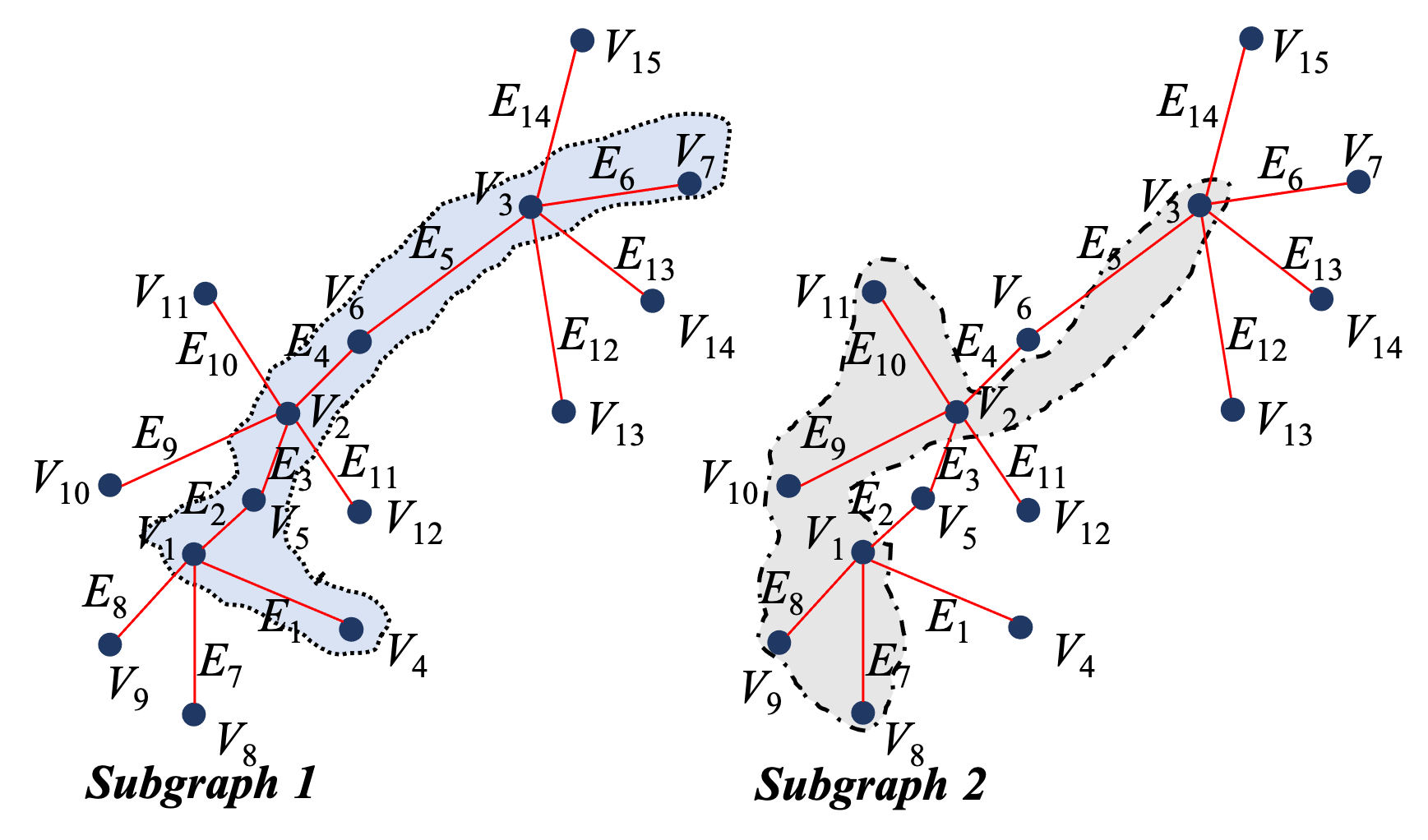
We illustrate the concept through an example in Fig. 8, showing a graph with vertices $\mathchar 29014_{\mathchar 28721}$ through $\mathchar 29014_{\mathchar 28721\mathchar 28725}$. The highest degree vertices are first brought into the cache, i.e., the input buffer: vertices $\mathchar 29014_{\mathchar 28721}$, $\mathchar 29014_{\mathchar 28722}$, and $\mathchar 29014_{\mathchar 28723}$ of degree 3, vertices $\mathchar 29014_{\mathchar 28725}$ and $\mathchar 29014_{\mathchar 28726}$ of degree 2, and then two vertices of degree 1, $\mathchar 29014_{\mathchar 28724}$ and $\mathchar 29014_{\mathchar 28727}$. The subgraph, Subgraph 1, consists of these vertices and edges $\mathchar 28997_{\mathchar 28721}$ to $\mathchar 28997_{\mathchar 28726}$ which connect them. After edges $\mathchar 28997_{\mathchar 28721}$ through $\mathchar 28997_{\mathchar 28726}$ are processed, vertices $\mathchar 29014_{\mathchar 28724}$ through $\mathchar 29014_{\mathchar 28727}$ have no unprocessed edges and may be replaced in the cache by $\mathchar 29014_{\mathchar 28728}$ through $\mathchar 29014_{\mathchar 28721\mathchar 28721}$ in Iteration 2. This creates Subgraph 2, the subgraph with edges $\mathchar 28997_{\mathchar 28727}$ through $\mathchar 28997_{\mathchar 28721\mathchar 28720}$), which is processed next, and so on.

The policy requires inexpensive preprocessing to sort vertices in order of their degrees. In practice, it is enough to sort vertices into bins based to their degrees, differentiating high-degree vertices from medium-/low-degree vertices to prioritize higher-degree vertices. After preprocessing, vertices of the input graph are stored contiguously in DRAM in descending degree order of the bins. are broken in dictionary order of vertex IDs. The key to avoiding random-access fetches from DRAM is the preprocessing step and the replacement policy.

We track the number of unprocessed edges, $\mathchar 28939_{\mathchar 29033}$ for vertex $\mathchar 29033$, decrementing it as each neighbor is processed. Initially $\mathchar 28939_{\mathchar 29033}$ is the vertex degree; when $\mathchar 28939_{\mathchar 29033}\mathchar 12349\mathchar 28720$, ${\bf\mathchar 29032}_{\mathchar 29033}^{\mathchar 29036}$ is fully computed. Tracking $\mathchar 28939_{\mathchar 29033}$ requires minimal hardware overhead (a decrementer and one word of storage per vertex), and its tracking enables GNNIE to maximize edge processing in each iteration.

Fig. 9 illustrates our policy, managed by a cache controller using a 4-way set associative cache. Graph vertices are stored contiguously in DRAM in descending degree order, where vertex 1 has the highest degree. If the input buffer capacity is $\mathchar 29038$ vertices, initially data (i.e., feature vector, connectivity information, $\mathchar 28939_{\mathchar 29033}$) for vertices 1 to $\mathchar 29038$ are loaded from DRAM.

The algorithm processes each such set of vertices in the input buffer in an iteration. This continues until all vertices are processed. At the end of iteration 1, i.e., after finishing computation of the subgraph corresponding to the first $\mathchar 29038$ vertices, if $\mathchar 28939_{\mathchar 29033}\mathchar 12604\mathchar 28941$ for any vertex, where $\mathchar 28941$ is a predefined threshold, it is replaced from the cache. We replace $\mathchar 29042$ vertices in each iteration using dictionary order if fewer (or more) than $\mathchar 29042$ candidates are available. These vertices are replaced in the input buffer by vertices $\delimiter 67273472\mathchar 29038\mathchar 8235\mathchar 28721\delimiter 84054785$ to $\delimiter 67273472\mathchar 29038\mathchar 8235\mathchar 28721\mathchar 8235\mathchar 29042\delimiter 84054785$ from DRAM: these have the next highest vertex degrees. For each such vertex $\mathchar 29033$, we write back the $\mathchar 28939_{\mathchar 29033}$ value into DRAM. When all vertices are processed once, we have completed a Round.

Similarly, the partial sums for the vertex feature vector in the output buffer are updated as more edges in the subgraphs are processed. Any ${\bf\mathchar 29032}_{\mathchar 29033}^{\mathchar 29036}$ for which all accumulations are complete is written back to DRAM. Due to limited output buffer capacity, and only a subset of partial vertex feature vector sums can be retained in the buffer, and the rest must be written to off-chip DRAM. To reduce the cost of off-chip access, we use a degree-based criterion for prioritizing writes to the output buffer vs. DRAM. As partial Aggregation results for softmax are written to DRAM, the numerator and denominator components for a vertex are stored nearby, for locality during future fetches.

Vertices evicted from the cache, with $\mathchar 28939_{\mathchar 29033}\mathchar 12604\mathchar 28941$, may be fetched again in a subsequent Round. Even in these Rounds, data blocks are brought into cache in serial order from DRAM: there are no random accesses from DRAM. During DRAM fetches, a cache block is skipped if all of its vertices are fully processed. The total unprocessed edges in a cache block is tracked through inexpensive hardware, similar to tracking $\mathchar 28939_{\mathchar 29033}$.

The effectiveness of the approach is illustrated in Fig. 10, which shows the histogram of $\mathchar 28939_{\mathchar 29033}$ distributions in the input buffer after each Round. The initial distribution corresponds to the power-law degree distribution, and in each successive Round, the histogram grows flatter – with both the peak frequency and maximum $\mathchar 28939$ becoming lower, thus mitigating the problems of power-law distribution. In contrast, HyGCN ignores the power-law problem, and AWB-GCN overcomes it using high inter-PE communication. Moreover, our approach is shown to be effective even for much more intensive GAT computations (prior accelerators do not address GATs).

Fig. 11 shows the impact of $\mathchar 28941$ on DRAM accesses for three datasets. As $\mathchar 28941$ increases, more vertices are evicted and may have to be brought back to the cache, resulting in more DRAM accesses. However, if $\mathchar 28941$ is too low, vertices may not be evicted from the cache, resulting in deadlock as new vertices cannot be brought in. In our experiments, we use a static value $\mathchar 28941\mathchar 12349\mathchar 28725$, but in practice, $\mathchar 28941$ may have to be changed dynamically when deadlock arises. Deadlock detection is inexpensive and is based on the number of total unprocessed edges in the partition, which is monitored by a counter, and this dynamic scheme will be inexpensive in hardware.

Software frameworks for GNNs include Deep Graph Library [34], AliGraph [39], and TensorFlow [1]. Some hardware accelerators have been proposed, but we know of no prior work that can handle networks that require softmax nonlinearities on graphs such as GATs. Although some GAT computations are addressed in [4], the crucial attention normalization step is left out. To our knowledge, no methods handle extreme input feature vector sparsity using graph-specific methods.

The HyGCN acclerator [38] uses an Aggregation engine for graph processing and a Combination engine for neural operations. This requires separate on-chip buffers for each engine: with workload imbalance at different stages of computation, these are not fully utilized. HyGCN must arbitrate off-chip memory access requests coming from on-chip buffers of two different engines, which involves complicated memory access control. Using a single hardware platform optimized to handle both the irregular graph computation and compute-intensive, albeit regular, DNN computation, GNNIE achieves performance gains over HyGCN. Moreover, HyGCN uses sharding with window sliding/shrinking to reduce random memory access during Aggregation: this has (1) limited efficacy for highly sparse adjacency matrices as the number of overlapping neighbors of vertices is a small farction of the total number of vertices in a shard, undermining its efficacy; moreover, no specific effort is made to address power-law degree distributions. (2) limited parallelism as the sliding window of the current shard depends on the shrinking of the previous shard; HyGCN does not fully leverage data reuse opportunities of high-degree vertices during Aggregation, performing $\delimiter 67273472\tilde{\mathchar 28993}\mathbf{\mathchar 29032}_{\mathchar 29033}^{\mathchar 29036\mathchar 8704\mathchar 28721}\delimiter 84054785\mathchar 29015^{\mathchar 29036}$, instead of cheaper $\tilde{\mathchar 28993}\delimiter 67273472\mathbf{\mathchar 29032}_{\mathchar 29033}^{\mathchar 29036\mathchar 8704\mathchar 28721}\mathchar 29015^{\mathchar 29036}\delimiter 84054785$, which is much cheaper [12, 22]. Moreover, input feature vector sparsity is not addressed and can result in stalls, resulting in computational inefficiency. These factors explain GNNIE’s high speedups (35$\mathchar 8706$ on average) over HyGCN.

AWB-GCN [12], which is limited only to GCNs and not general GNNs, views the problem as a set of matrix operations. It does not specifically try to reduce random memory accesses to the highly sparse graph adjacency matrix. Its dynamic scheduling scheme in AWB-GCN for workload redistribution among PEs may incur high inter-PE communication, degrading energy efficiency. EnGN [22] uses a ring-edge-reduce (RER) dataflow for Aggregation, where each PE broadcasts its data to other PEs in the same column. To reduce communication, EnGN reorders the edges, but this is an energy-intensive step, undermined by high sparsity in the adjacency matrix, that occurs frequently as the limited number of cached edges are replaced. The scheme has large preprocessing costs. Although EnGN attempts dimension-aware stage reordering to perform Aggregation or Weighting first, their results confirm that in practice, the Weighting-first scheme used in GNNIE is better.

Prior accelerators have not fully explored load balancing. Methods that offload tasks to idler PEs (ring-edge-reduce [22], multistage networks [12]) involve high communication and control overheads. GNNIE bypasses such approaches and uses the flexible MAC architecture for load balancing, using heterogeneous PEs, and assigning computation according to need. The idea is simple, effective, and easily implemented. It results in low inter-PE communication, low control overhead, and high speedup gain for the hardware overhead (Fig. 18). Preprocessing is cheap and involves linear-time binning of vertex features blocks into groups.

Frequency-based caching techniques for graph data have been proposed in [41] using a programming interface. However, [41] is a purely software-based framework, agnostic to the underlying hardware, for traditional graph analytics and uses a static approach. GNNIE uses a hardware-centric dynamic frequency-based caching scheme that tracks the $\mathchar 28939$ value for each vertex with minimal hardware overhead, and ensures serial access to DRAM. Other schemes are also static and more computational than GNNIE: they use hashing functions [6] or perform more computation [3, 35] in finding static communities/partitions that do not specifically address cache size. On the other hand, GNNIE’s computationally cheap dynamic scheme automatically adapts to the cache size using subgraphs built from vertices in the cache. GRASP [10], another cache management scheme for graph analytics, employs a most-recently-used (MRU) approach. However, this scheme is based on past history, while GNNIE’s use of the unprocessed vertex count measures future potential for a vertex.

References

- [1] https://www.tensorflow.org.
- [2] A. Aimar, H. Mostafa, E. Calabrese, A. Rios-Navarro, R. Tapiador-Morales, I.-A. Lungu, M. B. Milde, F. Corradi, A. Linares-Barranco, S.-C. Liu et al., “Nullhop: A Flexible Convolutional Neural Network Accelerator Based on Sparse Representations of Feature Maps,” IEEE Transactions on Neural Networks and Learning Systems, vol. 30, no. 3, pp. 644–656, 2018.
- [3] J. Arai, H. Shiokawa, T. Yamamuro, M. Onizuka, and S. Iwamura, “Rabbit Order: Just-in-time parallel reordering for fast graph analysis,” in Proceedings of the IEEE International Parallel and Distributed Processing Symposium (IPDPS), 2016, pp. 22–31.
- [4] A. Auten, M. Tomei, and R. Kumar, “Hardware Acceleration of Graph Neural Networks,” in Proceedings of ACM/IEEE Design Automation Conference, 2020.
- [5] J. Bruna, W. Zaremba, A. Szlam, and Y. LeCun, “Spectral Networks and Locally Connected Networks on Graphs,” in International Conference on Learning Representations, 2013.
- [6] X. Chen, Y. Wang, X. Xie, X. Hu, A. Basak, L. Liang, M. Yan, L. Deng, Y. Ding, Z. Du, and Y. Xie, “Rubik: A hierarchical architecture for efficient graph neural network training,” IEEE Transactions on Computer-Aided Design of Integrated Circuits and Systems, 2021.
- [7] Y.-H. Chen, T. Krishna, J. S. Emer, and V. Sze, “Eyeriss: An Energy-Efficient Reconfigurable Accelerator for Deep Convolutional Neural Networks,” IEEE Journal of Solid-State Circuits, vol. 52, no. 1, pp. 127–138, 2017.
- [8] G. Dai, Y. Chi, Y. Wang, and H. Yang, “FPGP: Graph Processing Framework on FPGA A Case Study of Breadth-First Search,” in Proceedings of the ACM/SIGDA International Symposium on Field-Programmable Gate Arrays, 2016, pp. 105–110.
- [9] M. Defferrard, X. Bresson, and P. Vandergheynst, “Convolutional Neural Networks on Graphs with Fast Localized Spectral Filtering,” in International Conference on Neural Information Processing Systems, 2016, pp. 3844–3852.
- [10] P. Faldu, J. Diamond, and B. Grot, “Domain-Specialized Cache Management for Graph Analytics,” in Proceedings of the IEEE International Symposium on High Performance Computer Architecture, 2020, pp. 234–248.
- [11] J. Fowers, K. Ovtcharov, K. Strauss, E. S. Chung, and G. Stitt, “A High Memory Bandwidth FPGA Accelerator for Sparse Matrix-Vector Multiplication,” in Proceedings of the IEEE International Symposium on Field-Programmable Custom Computing Machines, 2014, pp. 36–43.
- [12] T. Geng, A. Li, T. Wang, C. Wu, Y. Li, R. Shi, A. Tumeo, S. Che, S. Reinhardt, and M. Herbordt, “AWB-GCN: A Graph Convolutional Network Accelerator with Runtime Workload Rebalancing,” in Proceedings of the IEEE/ACM International Symposium on Microarchitecture, 2020.
- [13] T. J. Ham, L. Wu, N. Sundaram, N. Satish, and M. Martonosi, “Graphicionado: A High-Performance and Energy-Efficient Accelerator for Graph Analytics,” in Proceedings of the IEEE/ACM International Symposium on Microarchitecture, 2016, pp. 1–13.
- [14] W. Hamilton, Z. Ying, and J. Leskovec, “Inductive Representation Learning on Large Graphs,” in International Conference on Neural Information Processing Systems, 2017, pp. 1024–1034.
- [15] S. Han, X. Liu, H. Mao, J. Pu, A. Pedram, M. A. Horowitz, and W. J. Dally, “EIE: Efficient Inference Engine on Compressed Deep Neural Network,” in Proceedings of the ACM/IEEE Annual International Symposium on Computer Architecture, June 2016, pp. 243–254.
- [16] J. Hruska, “HBM2 vs. GDDR6: New Video Compares, Contrasts Memory Types,” https://www.extremetech.com/computing/289391-hbm2-vs-gddr6-new-video-compares-contrasts-memory-types, 4/11/2019.
- [17] N. P. Jouppi, C. Young, N. Patil, D. Patterson, G. Agrawal, R. Bajwa, S. Bates, S. Bhatia, N. Boden, A. Borchers, R. Boyle, P. Cantin, C. Chao, C. Clark, J. Coriell, M. Daley, M. Dau, J. Dean, B. Gelb, T. V. Ghaemmaghami, R. Gottipati, W. Gulland, R. Hagmann, C. R. Ho, D. Hogberg, J. Hu, R. Hundt, D. Hurt, J. Ibarz, A. Jaffey, A. Jaworski, A. Kaplan, H. Khaitan, D. Killebrew, A. Koch, N. Kumar, S. Lacy, J. Laudon, J. Law, D. Le, C. Leary, Z. Liu, K. Lucke, A. Lundin, G. MacKean, A. Maggiore, M. Mahony, K. Miller, R. Nagarajan, R. Narayanaswami, R. Ni, K. Nix, T. Norrie, M. Omernick, N. Penukonda, A. Phelps, J. Ross, M. Ross, A. Salek, E. Samadiani, C. Severn, G. Sizikov, M. Snelham, J. Souter, D. Steinberg, A. Swing, M. Tan, G. Thorson, B. Tian, H. Toma, E. Tuttle, V. Vasudevan, R. Walter, W. Wang, E. Wilcox, and D. H. Yoon, “In-datacenter Performance Analysis of a Tensor Processing Unit,” in Proceedings of the International Symposium on Computer Architecture, June 2017, pp. 1–12.
- [18] N. P. Jouppi, D. H. Yoon, G. Kurian, S. Li, N. Patil, J. Laudon, C. Young, and D. Patterson, “A Domain-Specific Supercomputer for Training Deep Neural Networks,” Communications of the ACM, vol. 63, no. 7, pp. 67–78, Jul. 2020.
- [19] S.-W. Jun, A. Wright, S. Zhang, S. Xu et al., “GraFBoost: Using accelerated flash storage for external graph analytics,” in Proceedings of the ACM/IEEE Annual International Symposium on Computer Architecture, 2018, pp. 411–424.
- [20] Y. Kim, W. Yang, and O. Mutlu, “Ramulator: A Fast and Extensible DRAM Simulator,” IEEE Computer Architecture Letters, vol. 15, no. 1, pp. 45–49, 2015.
- [21] T. N. Kipf and M. Welling, “Semi-Supervised Classification with Graph Convolutional Networks,” in International Conference on Learning Representations, 2017.
- [22] S. Liang, Y. Wang, C. Liu, L. He, L. Huawei, D. Xu, and X. Li, “EnGN: A High-Throughput and Energy-Efficient Accelerator for Large Graph Neural Networks,” IEEE Transactions on Computers, 2020.
- [23] J. Malicevic, B. Lepers, and W. Zwaenepoel, “Everything you always wanted to know about multicore graph processing but were afraid to ask,” in 2017 USENIX Annual Technical Conference (USENIXATC 17), 2017, pp. 631–643.
- [24] L. Nai, R. Hadidi, J. Sim, H. Kim, P. Kumar, and H. Kim, “GraphPIM: Enabling Instruction-Level PIM Offloading in Graph Computing Frameworks,” in Proceedings of the IEEE International Symposium on High Performance Computer Architecture, 2017, pp. 457–468.
- [25] P. Nilsson, A. U. R. Shaik, R. Gangarajaiah, and E. Hertz, “Hardware Implementation of the Exponential Function using Taylor Series,” in NORCHIP, 2014, pp. 1–4.
- [26] M. O’Connor, N. Chatterjee, D. Lee, J. Wilson, A. Agrawal, S. W. Keckler, and W. J. Dally, “Fine-Grained DRAM: Energy-Efficient DRAM for Extreme Bandwidth Systems,” in Proceedings of the IEEE/ACM International Symposium on Microarchitecture, 2017, pp. 41–54.
- [27] A. Parashar, M. Rhu, A. Mukkara, A. Puglielli, R. Venkatesan, B. Khailany, J. Emer, S. W. Keckler, and W. J. Dally, “SCNN: An Accelerator for Compressed-sparse Convolutional Neural Networks,” in ACM SIGARCH Computer Architecture News, vol. 45, no. 2, 2017, pp. 27–40.
- [28] D. Salomon, Data Compression: The Complete Reference, 4th ed. London, UK: Springer Science & Business Media, 2007.
- [29] P. Sen, G. Namata, M. Bilgic, L. Getoor, B. Galligher, and T. Eliassi-Rad, “Collective classification in network data,” AI magazine, vol. 29, no. 3, pp. 93–93, 2008.
- [30] H. Sharma, J. Park, N. Suda, L. Lai, B. Chau, V. Chandra, and H. Esmaeilzadeh, “Bit Fusion: Bit-Level Dynamically Composable Architecture for Accelerating Deep Neural Network,” in Proceedings of the International Symposium on Computer Architecture, June 2018, pp. 764–775.
- [31] N. Srivastava, H. Jin, J. Liu, D. Albonesi, and Z. Zhang, “MatRaptor: A Sparse-Sparse Matrix Multiplication Accelerator based on Row-Wise Product,” in Proceedings of the IEEE International Symposium on High Performance Computer Architecture, 2020, pp. 766–780.
- [32] N. Srivastava, H. Jin, S. Smith, H. Rong, D. Albonesi, and Z. Zhang, “Tensaurus: A Versatile Accelerator for Mixed Sparse-Dense Tensor Computations,” in Proceedings of the IEEE/ACM International Symposium on Microarchitecture, 2020, pp. 689–702.
- [33] P. Veličković, G. Cucurull, A. Casanova, A. Romero, P. Liò, and Y. Bengio, “Graph Attention Networks,” in International Conference on Learning Representations, 2018, pp. 1–12.
- [34] M. Wang, D. Zheng, Z. Ye, Q. Gan, M. Li, X. Song, J. Zhou, C. Ma, L. Yu, Y. Gai, T. Xiao, T. He, G. Karypis, J. Li, and Z. Zhang, “Deep Graph Library: A Graph-Centric, Highly-Performant Package for Graph Neural Networks,” 2020, arxiv/1909.01315.
- [35] Y. Wang, B. Feng, G. Li, S. Li, L. Deng, Y. Xie, and Y. Ding, “GNNAdvisor: An adaptive and efficient runtime system for GNN acceleration on GPUs,” in Proceedings of the USENIX Symposium on Operating Systems Design and Implementation (OSDI), Jul. 2021.
- [36] S. Ward-Foxton, “Memory Technologies Confront Edge AI’s Diverse Challenges,” https://www.eetimes.com/memory-technologies-confront-edge-ais-diverse-challenges, 9/18/2020.
- [37] K. Xu, W. Hu, J. Leskovec, and S. Jegelka, “How Powerful are Graph Neural Networks?” in International Conference on Learning Representations, 2019.
- [38] M. Yan, L. Deng, X. Hu, L. Liang, Y. Feng, X. Ye, Z. Zhang, D. Fan, and Y. Xie, “HyGCN: A GCN Accelerator with Hybrid Architecture,” in Proceedings of the IEEE International Symposium on High Performance Computer Architecture, 2020, pp. 15–29.
- [39] H. Yang, “AliGraph: A Comprehensive Graph Neural Network Platform,” in Proceedings of ACM SIGKDD International Conference on Knowledge Discovery & Data Mining, 2019, pp. 3165–3166.
- [40] R. Ying, J. You, C. Morris, X. Ren, W. L. Hamilton, and J. Leskovec, “Hierarchical Graph Representation Learning with Differentiable Pooling,” in International Conference on Neural Information Processing Systems, 2018.
- [41] Y. Zhang, V. Kiriansky, C. Mendis, S. Amarasinghe, and M. Zaharia, “Making Caches Work for Graph Analytics,” in IEEE International Conference on Big Data, 2017, pp. 293–302.