Statistical Mechanics of Floquet Quantum Matter: Exact and Emergent Conservation Laws
Abstract
Equilibrium statistical mechanics rests on the assumption of ergodic dynamics of a system modulo the conservation laws of local observables: extremization of entropy immediately gives Gibbs’ ensemble (GE) for energy conserving systems and a generalized version of it (GGE) when the number of local conserved quantities (LCQ) is more than one. Through the last decade, statistical mechanics has been extended to describe the late-time behaviour of periodically driven (Floquet) quantum matter starting from a generic state. The structure built on the fundamental assumptions of ergodicity and identification of the relevant “conservation laws” in this inherently non-equilibrium setting. More recently, it has been shown that the statistical mechanics has a much richer structure due to the existence of emergent conservation laws: these are approximate but stable conservation laws arising due to the drive, and are not present in the undriven system. Extensive numerical and analytical results support perpetual stability of these emergent (though approximate) conservation laws, probably even in the thermodynamic limit. This banks on the recent finding of a sharp ergodicity threshold for Floquet thermalization in clean, interacting non-integrable Floquet systems. This opens up a new possibility of stable Floquet engineering in such systems. This review intends to give a theoretical overview of these developments. We conclude by briefly surveying the current experimental scenario.
I Introduction
This is an introductory review of the statistical mechanics of periodically driven
closed quantum many-body systems, or quantum Floquet matter, developed through the last decade. By ‘close’ we mean it undergoes a pure Schrödinger evolution under a time-periodic Hamiltonian, hence its energy is not conserved. The statistical mechanics is for predicting the distribution of a
subsystem of the entire closed system (or, alternatively, describing the local operators).
The strategy of building a statistical mechanical description of the steady state of a complex many-body system consists of constructing the most unbiased distribution for the system respecting all the existing constraints. This requires identification of the relevant entropy functional, and then maximizing it subject to the constraints, which, for the purpose of a local description of a system, are the additive conservation laws. Hence the conservation laws are central to the approach described here.
The subject of Floquet physics has been existing since decades in various forms in various fields like condensed matter, quantum optics and atomic physics.
However, the statistical mechanics of periodically driven quantum matter took shape
only over the last decade. Within this period, the research area of Floquet quantum matter
exploded into a voluminous field. Reviewing every aspect of it is far from what this article aims, rather, the focus is on a very specific line of development – the statistical mechanics describing the late-time behaviour of Floquet quantum matter. In the question of organization, there are several finer classifications of the Floquet phases of matter (based on symmetry classes and other criteria), but in this overview we will focus on a broader classification based on the stability (against unbounded heating) and the underlying conservation laws responsible for it. A summary
of the view presented here
is given in Fig. 1.
II Equilibrium Statistical Mechanics and Thermalization: A short recapitulation via Information Theory
Statistical mechanics is a framework for describing the equilibrium states of matter, while Floquet matter is inherently out of equilibrium. Before making a concrete connection between the two apparently disparate subjects, in this section we recall some selected basics of equilibrium statistical mechanics and thermalization which appear useful in the context of Floquet matter. We resort to the information theoretic approach Jaynes 1957, since it provides the succinctness just right for our purpose.
II.1 Unbiased Statistical Distributions and Entropy
Suppose we know nothing about a variable , and we are asked to guess the normalized probability distribution
| (1) |
over a countable set of values can take. The most unbiased answer will obviously be – a flat distribution. We arrive at this conclusion by maximizing the uncertainty – since we have no information at all, our distribution should reflect that, and hence should be the one with most uncertainty/ignorance. Now suppose we have an additional constraint – we know that whatever the distribution is, it must give a preassigned value for the expectation of a particular quantity, say, i.e., must satisfy
| (2) |
Then what is the unbiased distribution in presence of this constraint? The answer will now be a distribution that maximizes the uncertainty, obeying the constraint (since we have no information about the distribution other than that the constrained is satisfied). In order to maximize uncertainty, we first need a sensible measure of uncertainty of the probability distribution. This was provided by Shannon Shannon 1948 via his entropy functional
| (3) |
where is a positive constant. (known as Shannon entropy) was shown to have the following properties Shannon 1948.
(a) It is a faithful measure of the uncertainty in – it increases monotonically with the uncertainty in
(b) It is always positive.
(c) It is additive: If we consider two separate non-interacting systems, then the total uncertainty of those two taken together should simply add up, and so do their individual s to give the
total
for the systems taken together.
It was also shown that the form of the functional given in Eq. 3 is the unique one to satisfy (a) - (c).
Accepting Shannon entropy as the measure of uncertainty in all we have to do is to maximize (extremization is usually sufficient) with respect to , modulo the constraint. This is a simple extremization problem, and can be solved using the standard method of Lagrange’s multiplier taking into account the two constraints in Eqs. (1) and (2), employing the corresponding Lagrange multipliers and respectively.
Extremizing
| (4) |
with respect to s immediately gives the desired distribution
| (5) |
where is the normalization factor, also known as the partition function.
Above can be applied to deduce the unbiased statistical distribution for a sub-system of a large physical system. The meaningful conserved quantities are the local conserved quantities (LCQ), represented by local operators. An operator is said to be local on a lattice if its real space representation is a product of onsite operators sitting on consecutive sites. We call a local operator non-local if is not a fixed number, but scales with the system-size. Intuitively, a local operator contains information only over a finite length scale ( consecutive sites) on the lattice. A local conserved quantity is additive for two large sub-subsystems of linear dimensions Such additive integrals of motion for the entire system (e.g. energy, particle number etc as applicable) are the quantities whose sharp average values characterize the distribution for the sub-system (see, e.g., Pathria 1972), and hence play the role of for it (here denotes the complete set of variables/observables necessary for defining the state of a sub-system). If energy is the only conserved quantity of interest, then Eq. 5 immediately gives the Gibbs’s distribution
| (6) |
where is the energy (Hamiltonian), being the Boltzmann constant (which we will set to unity henceforth), and being
the temperature.
If there are number of LCQs denoted by s, then the distribution is given by
| (7) |
and the ensuing ensemble is called the generalized Gibbs’ ensemble (GGE). In quantum mechanics, integrability is an ill defined concept, and hence
there is no concrete prescription to identify the conserved quantities that are relevant for constraining the distribution of the sub-system, except that additive LCQs are always bona fide
candidates. An ab-initio
numerical verification of GGE was first reported in Rigol et al. 2007 (see also Cassidy et al. 2011).
The statistical entropy of the sub-system is the classical uncertainty in the state of the sub-system (i.e., how mixed it is). This is quantified by the Von Neumann entropy or entanglement entropy (the latter follows from the fact that the entanglement between the sub-system and the rest of the system determines how mixed the state of the sub-system is – when the entanglement is zero, the sub-system is in a pure state). The Von Neumann entropy is given by
| (8) |
where is the density matrix of the sub-system, is the total number of states of the sub-system, and is the eigenvalues of corresponding to the eigenvector , and gives the probability of obtaining the sub-system in the state in a projective measurement done in the eigen-basis of The final expression of in Eq. 8 is exactly in the form of Shannon entropy (Eq. 3), and gives the measure of how mixed the state is: if it is a pure state, then for all except one, for which it is 1. then we get Thus, is basically the Shannon entropy characterizing the classical uncertainty in the state of the sub-system due to interaction with the rest of the system.
II.2 Thermalization and the Eigenstate Thermalization Hypothesis
Thermalization broadly means emergence of the thermal behaviour of a sub-system due to interaction with the rest of the system, in a generic many-body system (which, when kept isolated, has energy as the only LCQ). Usually it refers to a dynamical process, where the entire system is allowed to evolve from a non-thermal state, and the chaotic dynamics eventually allows a sub-system to explore its phase space within a narrow energy window fixed by the initial condition. After the steady state is reached, only thing we can guess about a sub-system is that it has a sharply defined average energy determined by the initial state, and following the deduction of Eq. 6, its statics will be given by a Gibbs’ distribution.
The last two decade have seen the development of a more
stringent concept of thermalization – it hypothesizes thermal behaviour
of a sub-system right at the level of the eigenstates of a closed quantum chaotic system. This Eigenstate thermalization hypothesis (ETH) Srednicki 1994; Rigol et al. 2016 says, for a generic interacting many-body quantum system, which has no other LCQ than energy, each eigenstate is thermalized to a temperature compatible with its energy density. In the strongest form, this amounts to saying that
when the whole system is in any of its eigenstates, the expectation values
of all local observables over the eigenstate equal to their respective
thermal average value corresponding to the temperature compatible with
the energy density of the eigenstate. In the parlance of information theory discussed above, this means that even being at an eigenstate, the system
provides enough fluctuations to its finite sub-systems – sufficient to render its state completely uncertain except fixing its energy. If there are more than
one conserved quantities that affects the statistical distribution of the
sub-system, then we likewise get a GGE (Eq. 7) in the eigenstate level. At its extreme lies the integrable systems, where there are as many relevant LCQs as there are degrees of freedoms, i.e.,
one has
Even at the level of ETH, the distributions are entirely determined based on (a) the assumption of ergodicity of a sort (albeit in the eigenstate level) and (b) the LCQs. This allows one to predict the long-time average behaviour of the local observables/sub-systems of a closed quantum chaotic system evolving from a typical initial state (a quantum quench), based only on the knowledge of the relevant conserved quantities as we discuss next.
II.3 Quantum Quenches, Diagonal Ensemble Averages (DEA) and Thermalization
We now focus on the late time behaviour of the state of a generic system that satisfies ETH. It can be argues that if is the Hamiltonian, and is the initial state, where are the eigenstates of corresponding to the eigenvalues (quasi-energies) then at a later time the expectation value of a local observable will be
| (9) |
The question is, whether it can approach an approximate steady value (with small fluctuations around it) at late times. Here, by late time we mean the time longer than that required for the transients to die down and the steady state to appear. Typically a time much longer than the inverse of the relevant spectral gaps (in proper units) qualifies. If a steady state is indeed reached, then this steady value must be equal to
| (10) |
which is obtained by dropping the explicitly time-dependent terms, i.e., by retaining only the terms in the above summation Rigol et al. 2016. The expression in Eq. 10 is exactly identical with the average of the obtained over the density matrix
| (11) |
which is diagonal in the eigen-basis of the Hamiltonian The density matrix described the so-called diagonal ensemble (DE), in which, the expectation values of the local operators are given by classical averaging (i.e., with real positive weights – no interference) over their expectation values on the eigenstates of Thus, in some sense, it is sufficient to know the properties of the eigenstates of and their initial weights to determine the long-term behaviour.
The question then is, whether dropping the phases and time dependence is a valid approximation at late times (clearly it cannot be so at early times where the state is still closed to the initial state which can have a strong phase coherence in the eigen-basis ). Loosely speaking, at late times, as the phase oscillates increasing faster, and unless the contribution is cancelled out when summed over as they pick up opposite signs randomly – just in the spirit of Riemann–Lebesgue lemma for oscillatory integrals Gradshteyn and Ryzhik 2007. This process of losing phase information is often referred to as dephasing.
It should be noted that this dephasing requires significant contributions in the sum in Eq. 9 for several close by values of and . If there are only a few terms on the right hand side of Eq. 9, then one obtains a sustained oscillation with a few frequencies, and not a steady state described by a DE. This happens if either the initial state expanded in terms of the eigen-basis has only a few terms, or is a non-local projector, which, when applied on projects out only a few eigenstates. With a typical initial state and a local operator, none of the above is likely to happen for any physical (local, short-ranged) Hamiltonian, and hence one can expect a diagonal ensemble at late times. The locality of is hence a sufficient condition for getting DE for a generic initial state at late times.
A more elaborate analysis shows, that for a generic and a local observable the state of the system at late times is extremely well approximated (indistinguishable within any realistic experimental resolution) by the DE for overwhelming majority of time during its evolution Reimann 2008.
This is already a heavily approximated description, since we have thrown away the information in the phases and the cross terms, however, this still requires knowledge of exponentially many (in ) initial information (the weights s) to construct the ensemble. Now if additionally assume that the expectation value of any local observable over the energy eigenstates is a smooth function of the energy, then for an initial state with a very narrow energy variance, it is easy to see that the diagonal ensemble is nothing but the microcanonical ensemble for the whole system Rigol et al. 2016:
| (12) |
where is the mean energy of the initial state. This is obtained by assuming the width of the initial state is very narrow in energy (and hence, by ETH, in every local observable), and we can approximate all the expectation values within the sum by that for a single eigenstate with energy This implies, the effective steady density operator for a finite sub-system at late times will be given by
| (13) |
where the operation implies tracing over the rest of the system leaving out the finite sub-system. The “” symbol can be replaced by the “” sign in the thermodynamic limit. Now assuming that energy is the only quantity without fluctuations for the whole system when it is in the eigenstate , the only relevant independent constraint for the sub-system distribution is that the energy of the sub-system value should be fixed to sharp value consistent with Then the maximization of Von Newman entropy immediately gives (see, e.g. Jaynes 1957)
| (14) |
where is the bulk Hamiltonian of the sub-system, and is its partition function. The effective temperature can be determined self-consistently from the equation
| (15) |
It is important to note that obtaining the canonical ensemble from the microcanincal one rests on the assumption that the interactions are short-ranged, and while estimating energy we can neglect the boundary effects in surface to volume ratio, which vanishes in the thermodynamic limit. Hence this does not apply
prima facie to systems with sufficiently long-ranged interactions.
For an integrable system with LCQs, the late time behaviour will hence be given by a GGE:
| (16) |
where are LCQs contained within
the sub-system.
Next we discuss the basics of Floquet quantum matter and how to apply the above to characterize its late time behaviour.
III Floquet Quantum Matter and its Statistical Mechanics
III.1 Steady States of Floquet Matter
We begin with the precise definition of Floquet quantum matter.
It is essentially a closed quantum many-body system driven periodically in time.
In most cases, it is considered to be in a pure state at all time.
The dynamics of the entire system is also deterministic. The statistical description hence applies, as usual, only to a finite sub-system of the whole system, or, in other words, only for describing local operators as it is for the equilibrium
(time-independent ) case discussed above.
Given the above definition, closed Floquet matter is inherently out-of-equilibrium, hence applying the idea of equilibrium statistical mechanics to it might apparently look antithetical. So it did till the beginning of the last decade – to the least, one has to have a non-trivial stable steady state to describe, but the common wisdom was, a periodically driven system with many degrees of freedom should keep on absorbing energy without bound (as, for example, suggested by Fermi’s Golden rule) and will tend to a completely featureless random state asymptotically, since energy itself is not conserved.
However, it turns out not to be the entire story – it was shown, the polarization of an infinite integrable spin chain can remain dynamically frozen arbitrarily close to its initial state at all time under simple periodic drive, if the drive is sufficiently strong and fast Das 2010. The freezing is a non-monotonic function of the drive frequency and the amplitude, and is almost perfect under certain drive conditions. We will see the most interesting aspect of the freezing is probably that it is approximate, but perpetually stable. But from statistical mechanics point of view, the most important aspect is, the freezing is independent of the initial state. The phenomenon thus heralded the existence of a
equilibrium ensemble-like description of Floquet quantum matter.
The phenomenon was later dubbed as dynamical many-body freezing (DMF) Bhattacharyya et al. 2012; Hegde et al. 2014; Mondal et al. 2012; Russomanno et al. 2012; Das and Moessner 2012; Bastidas et al. 2012a; Bastidas et al. 2012b; D’Alessio and Polkovnikov 2013; Agarwala et al. 2016; Mukherjee et al. 2020; Ghosh et al. 2020,and is basically a many-body version
of long-known single-particle phenomenon of dynamical localization Dunlap and Kenkre 1986; Grossmann et al. 1991. Most importantly, DMF has recently been shown to persist for a large class of non-integrable interacting systems with the undriven part containing Ising or two-body Heisenberg interactions of virtually any kind, and on lattices of any dimension Haldar et al. 2021. Stability of DMF entails an approximate emergent conservation law. Subsequent works showed, non-trivial steady states are generic to non-interacting Floquet matter due to presence of exact conservation laws Lazarides et al. 2014a.
III.2 From Floquet to Quantum Quenches
The connection between the late-time behaviour of quantum Floquet matter and quantum quenches with time-independent Hamiltonian (and hence with the ensemble picture describing their late time behaviour) becomes apparent if one observes a Floquet system stroboscopically. Floquet quantum matter is described by a time-periodic many-body Hamiltonian
| (17) |
The time-evolution operator can be cast in the form (Floquet-Bloch theorem, see, e.g. Mostafazadeh 1998)
| (18) |
where denotes the time evolution operator for evolution from to is a time-independent hermitian operator (often called Floquet Hamiltonian), the Identity operator, and an integer. All the information of the stroboscopic dynamics is stored in and contains the information about the dynamics within a period (so-called micromotion). Now if one focuses only on stroboscopic observations at discrete moments given by (i.e., after complete cycles), then the states will be given by
| (19) |
This would also exactly be the state at if the evolution was carried out by the time-independent Hamiltonian Eq. 19 thus maps the evolution of a Floquet system to a quench problem with the time-independent Hamiltonian under stroboscopic observations, where
| (20) |
being hermitian, its eigenstates (Floquet states) with eigenvalues can be ortho-normalized to form a complete basis known as Floquet basis. Note that are also eigenstates of with eigenvalues
These basis plays a role similar to that played by the energy eigen-basis in time-evolution under a time-independent Hamiltonian.
We are now equipped to apply all the constructs and concepts discussed in the previous section (Sec. II) to describe the late time behaviour of Floquet matters. The rest of the review is tailored to answer questions laid down in the beginning of this subsection.
III.3 Periodic Steady State and Synchronization
The first question concerns emergence of a steady state of some sort in Floquet matter at late times. The argument of dephasing in Sec. II implies that at late times, the a generic Floquet system starting from a generic initial state will execute a periodic variation with time, synchronized with the drive. To see this, let us consider a periodic drive as discussed above. Let us expand a generic initial state
| (21) |
where are the Floquet eigenstates. Then, since when observed at instants the state will be exactly the one obtained due to evolution with the time-independent Hamiltonian corresponding to the for the given problem, (see Eqs. 19-20) we expect, following Eq, 10, for
| (22) |
Here the superscript“” indicates that we have considered the stroboscopic observation series . For this series, as we see, is expected to attain a time-independent value. Now instead of the series we could have taken the series where and carry out the above arguments exactly in the same way, only, now taking as our starting instant – is replaced by and by This immediately implies at late time, for
| (23) |
for every Here are the eigenstates of with eigenvalues (the eigenvalues are independent of ). Eq. 23 implies that the variation of the DE average of a local observable over a period given by as runs from to will be the same over the next period as runs from to In other words, get synchronized with the drive at late times – this is the Floquet “steady state.”
III.4 Floquet Dynamics vs Quantum Quench with a Local Hamiltonian: Looking Through the Magnus glass
From the viewpoint of a late-time behaviour, the main difference between quench
with a natural physical (local, short-ranged) time-independent Hamiltonian
and stroboscopic Floquet dynamics with an lies in some crucial differences
possible between the structure of and . Even when the periodically driven
Hamiltonian (which gives rise to ) is a 2-local, short-ranged Hamiltonian,
can have the following exotic properties. (a) can be long-ranged, even infinite ranged.
(b) For low drive frequency can contain substantially strong multi-body
(local, with ) interactions, and can even be non-local.
These properties can naturally make the eigenstates of
very different from the eigenstates of a standard and hence can produce a diagonal ensemble with drastically different properties from a diagonal ensemble with
There are several ways of calculating (see, e.g., Goldman and Dalibard 2014; Bukov et al. 2015a; Eckardt and Anisimovas 2015). A rather transparent and popular one is the Magnus expansion Magnus 1954 (see also Bukov et al. 2015a). This is a series expansion for in ( is the drive frequency). Magnus expansion is given in terms of nested commutators between the drive Hamiltonian at different instants as follows.
| (24) | |||||
An interesting thing about Magnus expansion is, it is hermitian at every order. Magnus expansion
provides a way to derive a sufficient condition for absence of unbounded heating and stability of Floquet matter.
If is a many-body Hamiltonian, then in the thermodynamic limit the radius of
convergence of the above expansion is usually zero Kato 1976. However, under special circumstances
this series can be shown to converge or to be asymptotic. Those are the cases where the stability of a
Floquet phase can be guaranteed. The conserved quantities relevant for
constructing the statistical mechanics for a Floquet system are local operators which
commutes with Also, the symmetries of are the symmetries that
characterize the Floquet phases.
In the rest of the article we will review the existence and nature of Floquet ensembles and the conservation laws characterizing them. Based on the nature of stability, three broad classes of Floquet matter have been discussed most widely – the non-interacting, the clean interacting, and the MBL, to which we will limit our discussions.
At this point it seems useful to clarify two important concepts, namely,
ergodicity and emergent conservation laws, especially the sense
in which they are used here.
First, we are using the word ergodicity in a more inclusive sense here
– by it we mean the dynamics and/or eigenstate properties (e.g. in ETH) are such that
the correct statistical distribution (for the sub-system observables)
maximizes the entropy respecting all exact conservation laws for local operators.
Second is the idea of emergent conservation laws. In the Floquet context, exact conservation laws may trivially be inherited from the
drive Hamiltonian broadly through three different ways – either due to the symmetries in ,
or owing to its integrability, or due to disorders (e.g., bits in MBL systems, see e.g. Abanin et al. 2019; Imbrie et al. 2017). In addition to those, there may arise further constraints due to the dynamics,
which can sometimes take the form of approximate LCQs. These emergent LCQs have no trivial
origin that can be guessed looking at at any given instant. They can often leave legible foot-prints on
but since convergent series for usually do not exist for any non-trivial many-body system,
they are hard to guess even from in general. Hence, while constructing the ensemble by maximizing the entropy, those are left out (only exact conserved quantities are taken into account).
Hence they break the ergodicity of a system in a surprising manner. An algorithm to
identify the emergent conservation laws and incorporating them in constructing statistical distributions is an important open problem in the way of constructing a complete statistical mechanics for describing
late time behaviour of complex dynamical systems. Until this problem is
solved, we are in an rather uncomfortable position: our ensemble
description could be incomplete, and ergodicity could be found broken
in an unexpected way by some ad hoc emergent conservation law. We will see, these emergent conservation laws are responsible for non-trivial late-time behaviour of interacting Floquet matter initialized to generic initial conditions. Fig. 1 charts out a broad (though incomplete) classification of
Floquet matters based on their stability and associated LCQs. We will roughly follow the flow of the diagram for the rest of the review.
IV Non-interacting Floquet Matter
IV.1 The Generalized Periodic Gibbs’ Ensemble (PGE) and its conservation laws
The stability of the polarization of an integrable Ising chain Das 2010 (which can be mapped to free fermions) under periodic drive raised the question of the role of integrability and the possibility of existence of some sort of conservation laws in such systems, that prevent unbounded heating (though energy itself is not conserved). It was shown Lazarides et al. 2014a that a general integrable system constituting of free fermions (or one that can be reduced to free fermions), when driven periodically, indeed hosts an extensive number of -periodic LCQs A general non-interacting fermionic Hamiltonian of the form
| (25) |
was considered, where are fermionic, and are complex matrices. For one dimensional lattice, can also be hardcore bosons. Now the key observation is, given the nested commutator structure of the Magnus expansion of (Eq. 24), if is bi-linear in fermions, so if Thus, in principle, using a unitary transformation (see, e.g., Suzuki et al. 2013) one can always reduce to a free fermionic Hamiltonian of the form
| (26) |
Note that the operators ’s can be quite complicated in terms of the original degrees of freedom, but the final result is still bi-linear since the algebra closes in each order of the expansion. The operators
| (27) |
are relevant (2-local) periodically conserved quantities for the stroboscopic steady series One can explicitly construct time-periodic quantities, that will be stroboscopically conserved, i.e. and hence will be useful for constructing the synchronized ensemble. The prescription is
| (28) |
for all This completes the list of ingredients to construct the ensemble that represents the late-time synchronized state of the integrable Floquet matter described above. We then just follow the statistical mechanics prescription given in Eq. 16 to construct the ensemble. The ensemble thus constructed is termed as (generalized) Periodic Gibbs’ Ensemble (PGE) Lazarides et al. 2014a. It is given by the density operator
| (29) |
where the s are fixed by requiring that
| (30) |
where is a time-independent normalization factor analogous to the
partition-function.
The density operator has the following two properties. (a) It correctly gives the conserved quantities.
(b) Since the are periodic in time, is itself manifestly periodic in time:
in conformation the synchronized steady state.
The description hence requires the values of only conserved quantities,
rather than numbers to specify the initial conditions exactly.
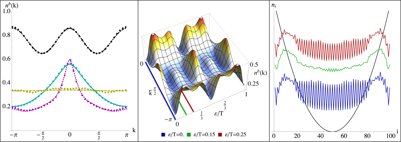
We end this section by demonstrating the predictive power of PGE. The accuracy of the PGE is demonstrated by comparison with exact numerical result for an experimentally relevant system of hardcore-bosons on a one-dimensional lattice given by the Hamiltonian Lazarides et al. 2014a
| (31) |
Here are hardcore-bosons (HCBs) obeying bosonic commutation relations off-site, with
additional hardcore condition onsite.
A Jordan-Wigner transformation, with
, maps
to Eq. (25) with
, and fermionic commutation relations for the .
The driven terms are, a time-dependent super-lattice potential superposed on a quadratic potential, and a time-dependent hopping amplitude with . The protocol used here consists of preparing the system in the ground state in the presence of a harmonic potential , fixing . This allows taking the thermodynamic limit, since for large total number of particles the dimensionless parameter Rigol and Muramatsu 2004 plays a role analogous to the density in the uniform limit. Results with different system sizes but constant are therefore comparable.
At time , the driving is switched on so that the total Hamiltonian is
with .
Considering the experimentally accessible momentum distribution
of the bosons, a numerical method consisting of solving the
fermionic time-dependent problem and, in the end, inverting the Jordan-Wigner
transformation was employed.
We demonstrate various periodic states corresponding to different sets of values of the parameters of the model. The leftmost panel of Figure 2 shows snapshots of the PGE momentum distribution
| (32) |
at late time (after cycle). The dashes lines are the PGE prediction, while the points are exact numerical
results. The agreement between the both resoundingly confirms the validity of the PGE picture at late times.
It is to be noted that at low-frequency regime, as expected, the corresponding time-averaged Hamiltonian Eckardt and Anisimovas 2015 is not an appropriate description. As a striking illustration, the black line shows a momentum distribution with peaks at the edges of the Brillouin zone. The central panel shows the time evolution of the momentum distribution over an entire period corresponding to the parameters associated with the cyan line in the left frame. Of course, the system evolves through states in which the momentum is peaked
at different locations of the Brillouin zone.
Finally, the rightmost panel shows three snapshots of the
density distribution of the same system at times indicated by the coloured
lines (black, green and red) in the central panel. The high frequency spatial oscillations and the peaking of the density at the edges is also very different from what would be obtained had the system been well-described by a
time-averaged Hamiltonian, since the time-averaged potential (shown in black) is smooth and peaks at the edges.
IV.2 Dynamical Many-body Freezing (DMF) and An Emergent Conservation Law in Non-interacting Floquet Matter
For non-interacting Floquet matter, as we have just seen, there are number of relevant periodic conserved quantities. Hence ergodicity in such system would mean a distribution that respects all those conservation laws, and no other constraints – exact or approximate – at late times. This gives us the PGE (Eq. 29).
However, already before the inception of the ideas of PGE and its exact conservation laws, it was shown, the ergodicity thus defined can be broken by emergence of a conserved quantity when the drive is sufficiently strong Das 2010. The following strongly driven integrable quantum Ising chain was considered
| (33) |
(
is the driving field and
are component of the Pauli spin sitting at site ).
The above Hamiltonian can be reduced to that of free fermions and can be cast in the form of Eq. 25 using Jordan-Wigner
transformation (see, e.g., Suzuki et al. 2013), hence should be completely
described by a PGE with exact conserved quantities. However, as
discussed below, that turns out not quite to be the case.
In the fast drive regime, starting from a highly polarized initial state the polarization acquires an steady average value depending on the drive amplitude and frequency , about which it fluctuates. In the limit, for average over infinite time, the time-averaged magnetization can be captured under a rotating-wave approximation Das 2010 by
| (34) |
where is the ordinary Bessel function of order From this, we see, for certain specific values of and satisfying the peak freezing condition:
| (35) |
the system remains maximally frozen with Similar freezing is also obtained for square-pulse drive ( is the Signum function), applied on the same model – just the condition for the peak freezing becomes
| (36) |
In these systems, there is clearly an approximate emergent
conserved quantity, namely, This is certainly a strong constraint in additional to the exactly conserved stroboscopic quantities s and evidently independent of them. This thus breaks the ergodicity further in this integrable system: the PGE, which does not include by construction, is hence not an adequate local description for the system. We will see, in the presence of non-integrable interactions (quantum-chaotic many-body systems) while the exact local conservation
laws disappear, the emergent conservation laws survive and continues to shape the statistical
mechanics of the steady state, especially, preventing it from attaining the featureless, locally infinite-temperature like state.
IV.3 Infinite-Temperature like Scenario in Integrable Floquet Matter:
We conclude this section with interesting results underscoring the
non-triviality of DMF in the above integrable systems. These systems
can actually be driven to locally infinite-temperature
ensemble under slow enough periodic drive Ishii et al. 2018!
Despite the existence of local conservation laws,
this happens at low enough when the Magnus expansion fails to converge in any local basis
(i.e., basis which is formed by the complete ortho-normal set of eigenstates of some local operator).
In that case, though the conserved quantities exist, they are unable
to constrain the statistical
distribution (Eq. 29), since in that case one
obtains for all , rendering (the identity operator), representing an infinite-temperature state.
Finally, it is noteworthy that phase coherence throughout the dynamics is crucial for the stability of the extensive number of conservation laws in a non-interacting system. It was shown that even in a non-interacting translationally invariant system, which can be mapped to a bunch of decoupled two-level systems in the momentum space, can thermalize to infinite temperature (each of the two level systems approach a state with equal probability for the two levels, and hence of maximum entropy) if the Stückelberg-like phases are randomized or discarded by hand after each half-cycle, and transition probabilities are used instead of amplitudes to calculate the probabilities after every cycle Hegde et al. 2014; Mukherjee et al. 2008. The locally infinite-temperature like state is approached exponentially fast with number of drive cycles. This shows the stability of the periodic conservation laws depends crucially on the coherence of the repeated quantum interference taking place over cycles.
V Interacting Floquet Matter under Moderate Drive: Floquet ETH and the Late-time Ensemble

Suppose a generic interacting non-integrable many-body system without disorder and localization is subjected to moderate periodic drive (i.e.,
the drive amplitude and frequency are comparable with the other
couplings in ). In such a system, the energy is not conserved, and since there is no underlying integrability, there is no obvious (periodic) conserved quantities to constraint the dynamics. This implies,
the system will keep on absorbing energy without bound, and will asymptotically approach a state which looks locally like an infinite-temperature state.
This picture is consistent with our common intuition about a closed Floquet system which does not dissipate
out its energy, as reflected, say by Fermi’s Golden rule for periodically
perturbed quantum systems with continuous spectrum (see, e.g. Sakurai 1994). For systems with finite spectral width, the energy absorption will stop, but
for any generic initial state, the final state will be a random superposition
of all states in any local basis. This means, each Floquet eigenstate
must be thermalized to infinite temperature! This Floquet ETH picture was proposed and verified for generic Hamiltonian irrespective of the form of the drive as long as it is moderate D’Alessio and Rigol 2014a; Lazarides et al. 2014b; Ponte et al. 2015a.
Of course, one should keep in mind that even a
quantum-chaotic time-periodic Hamiltonian
can have symmetries which it respects at all time, hence should also
respect those symmetries. In such a case, the chaotic hybridization of states due to the drive will hence happen only within each such symmetry sector, and not across them. Obviously, in that case,
the quantities whose conservation are protected by the symmetry will not
exhibit Floquet thermalization.
For illustration, in Lazarides et al. 2014b, a non-integrable model of hardcore bosons on a lattice given by the Hamiltonian
| (37) | |||||
has been considered,
with a time-periodic potential
with for and
for ().
In particular, taking the above Hamiltonian as an example,
it was shown that expectation value (eigenstate expectation values or EEV) of a
local operator over all the Floquet eigenstates
are almost same, with negligible state-to-state fluctuations across the spectrum (Fig. 4).
It shows that EEV for every Floquet state is almost same (a very narrow distribution., whose width was shown to vanish with
increasing ), and are almost equal to the infinite temperature average.
The consequence of this on the late-time behaviour was also demonstrated in Lazarides et al. 2014b. For a generic initial state the late-time expectation value of a local observable will be given by Eq. 22. Now according to Floquet ETH, that for every we have
| (38) |
where is the infinite-temperature average. Then, Eq 22 immediately gives,
| (39) |
regardless of the specifics of the initial state and also the
details of the Hamiltonian (since Floquet ETH is expected to hold for
any generic Hamiltonian). This is demonstrated
in Fig. 5 for the Hamiltonian in Eq. 37.
Floquet ETH and :
Floquet ETH will require to be a non-local operator –
otherwise itself will serve as a stroboscopically conserved local
operator, and the local description will be a Gibbs’ ensemble
with a serving as a local Hamiltonian, rather than an
infinite temperature ensemble. Any series expansion of in terms
of local operators hence must not converge.
Else one can obtain a controlled approximation for and using that, an approximate Gibbs’ distribution. This, of course, is a necessary but not sufficient
condition for an unbounded Floquet heating.
Floquet Prethermalization We conclude this section briefly mentioning an ephemeral but experimentally relevant phase of Floquet matter, namely, the prethermal phase. It was shown that the phenomenon of prethermalization (see, e.g., Berges et al. 2004; Gring et al. 2012; Essler et al. 2014; Mallayya et al. 2019), i.e., existence of a substantial time interval needed by an interacting, non-integrable many-body system to exhibit the chaotic dynamics in its relaxation behaviour starting from an atypical initial state, also persists for Floquet systems Canovi et al. 2016; Mallayya and Rigol 2019. In the early settings, prethermalization was shown for weakly interacting models which are in proximity with integrable ones: after switching on the integrability breaking interaction to an integrable Floquet system, the dynamics of the system continues respecting the periodic conservation laws (and the PGE) pertaining to the integrable system till some time After that, the system thermalizes steadily. Later it was shown, prethermalization does not necessarily occur only in systems close to integrability, but can exhibit memories of an atypical initial state for a long characteristic time in any generic system under fast drive Kuwahara et al. 2016; Mori et al. 2016; Abanin et al. 2017; Weidinger and Knap 2017; Machado et al. 2019; Luitz et al. 2020; Bukov et al. 2015b, and even in some slowly driven systems De Roeck and Verreet 2019. Such prethermal Floquet states can host interesting though metastable phases of quantum matter, and can often be described by a PGE Canovi et al. 2016, or a thermal (Gibbs) ensemble Machado et al. 2019, or even some interesting non-thermal phases Luitz et al. 2020; Ho and De Roeck 2020. These phases can be of considerable practical interest from a viewpoint of contemporary experiments – perfect quantum dynamics can be simulated only for a finite, rather short durations, after which several unavoidable imperfections that entail a real-life setup will anyway bring in decoherence. If the life-time of a prethermal phase is comparable with the experimentally allowed time-windows, it is as good as a stable phase from experimental perspective. Of course, a long-lived prethermal phase also appears generically when the drive amplitude is below a threshold Ji and Fine 2018.
In the next section we will see, stable Floquet states are possible in clean, interacting non-integrable systems if the drive is strong enough.
VI Strongly Driven Clean Interacting Floquet Matter and The Absence of Unbounded Heating
VI.1 Floquet Thermalization Threshold
The locally infinite-temperature like scenario that pertains to Floquet-ETH in interacting systems under moderate drive, undergoes a sharp qualitative change as the drive amplitude is increased. Beyond a sharp threshold value of the drive amplitude, it shows a strong memory of its initial state Haldar et al. 2018. The model taken for illustration is given by the periodic Hamiltonian
| (40) |
with
| (41) |
The s are Pauli matrices. The chain has periodic boundary condition, but
the translational invariance is tampered with, by putting
and
This choice was to break all obvious symmetries.
In presence of the transverse field, the
the static part
of the Hamiltonian
is known to be ergodic due to the four-fermionic interaction terms arising from the next-nearest neighbour interactions under the spin to fermion mapping, and also due to the longitudinal field.
Under the periodic drive with the amplitude above a sharp threshold, the system shows
strong freezing, while below the threshold it’s behaviour is consistent with Floquet thermalization to a locally infinite temperature state. This has been shown in Fig. 6.
Interestingly, as emphasized in the rightmost frame of the Fig., the threshold value shows no perceptible dependence on the system-size The infinite drive-time limit ( as ) is captured by taking the diagonal ensemble average in the Floquet basis (see, Eq. 22).
VI.2 Dynamical Many-body Freezing and The Emergent Conservation Law in Clean Floquet Matter

Dynamical Freezing: It was shown that the absence of thermalization and strong freezing is actually a manifestation of an emergent conservation law. Just as it is in case of integrable Ising chain Das 2010, here the magnetization emerges as an approximately conserved quantity under the drive with strength beyond the threshold. The conservation (freezing in the language of Ref. Das 2010 – see Sec. IV.2) becomes perfect (peak freezing) under the drive condition
| (42) |
( is an integer)
as can be seen from the exact numerical results (Fig. 7, left frame) for natural
(fully polarized) and generic (high temperature) initial states. This is also obtained from
various analytical methods outlined in the following sections.
This peak freezing
condition is identical to that obtained for integrable Ising chain under square drive Bhattacharyya et al. 2012 (Eq. 36).
Nature of the Conservation Law and Sub-system Entropy
This can be gleaned from the expectation value of over the Floquet eigenstates arranged in decreasing order of their value, against their label (in the same order) normalized by the Hilbert-space dimension
as shown in Fig. 8. These are compared for various values of the drive amplitude
against the step-structure obtained by similarly arranging the eigenvalue of for its unentangled eigenstates - we call them the basis states (these are the simultaneous eigenstates of all )
The result show, for which is above the threshold (the threshold is see Fig. 6(c)), the magnetization of the Floquet eigenstates are almost indistinguishable from the magnetization of the eigenstates
of in a one-to-one correspondence, which means that the Floquet eigenstates are at most hybridization of the basis states with the same eigenvalues for , but not a superposition of them with different eigenvalues of . In other words, each Floquet state is an eigenstates of though they are free to delocalize within a given
eigen subspace of The Hilbert space is thus fractured into disjoint eigen subspaces of and it emerges as a conserved quantity (Fig.9). As is reduced and the
threshold is approached, the step structure smooths out, indicating hybridization of basis states (), and below the threshold () it flattens out completely to zero, indicating all the Floquet states are locally thermalized to infinite temperature.
Whether conservation of alone suffices to determine the ensemble, i.e.
whether is an accurate description
of the Floquet ensemble is still an open question. In particular, this seems not to be the entire picture away from the peak freezing points. There is only approximately conserved. The constraints and their nature are yet to be identified. To a first approximation, the constraint consists of a local Hamiltonian given by the first few terms of the moving frame Magnus expansion away from the freezing peak, assuming the expansion is asymptotic. Further investigation in this direction is in progress.
The effect of the emergent conservation law on the growth of sub-system entropy
has been illustrated in Ref. Haldar et al. 2021. The evolution of the half-chain entanglement was tracked, taking various basis states belonging to different eigen-subspaces of of various sizes as the initial states. The entropy growth reflects the nature of the conservation - it is not that
the system remains close to an basis state because is large compared to other scales in the problem. In fact, most of the basis states will evolve substantially to generate extensive
sub-system entropy, while some will not. What is respected, is the
global conservation of
the dynamics spreads an basis state only within its own eigen-subspace corresponding to the same eigenvalue of
For example, a fully polarized state is the only member of the subspace with , hence taking this as a initial state shows no entanglement growth even after million drive cycles. But taking any basis state with (e.g., a Néel ordered state) results in substantial growth of the entanglement, since the sector has several members over which the evolving state can delocalize.
VI.3 Stability of the Conservation Laws and the Thermodynamic Limit
Stable Floquet states have been observed numerically under moderate drive
in various clean interacting finite-size systems Agarwala and Sen 2017; Dasgupta et al. 2015; Qin and Hofstetter 2018; Seetharam et al. 2018; Prosen 1998; Prosen 2002; Luitz et al. 2018. However, no evidence of stability was reported for those moderately driven systems in the large limit (see, also Luitz et al. 2017).
As already mentioned above, the situation changes drastically if the drive amplitude crosses a threshold strength Haldar et al. 2018. A systematic finite-size analysis of the stability of was made for various interacting non-integrable models - Ising and Heisenberg spins with interactions of various ranges and locality (including three spins interactions). None of them shows any discernible decline in the conservation with the system-size Haldar et al. 2021. Moreover,
for a large class of models (Ising and Heisenberg interactions of virtually any kind and in any lattice dimension in the static Hamiltonian),
it was shown that a moving frame Magnus expansion for (applies independent of hence holds as ) is an asymptotic expansion, and it is consistent with the stability
of observed from the finite size analysis of the exact numerical results. That is an indicative of the survival of the conservation in the limit, though this is certainly not a conclusive proof of the same.
Finally, it is worth emphasizing that the stability of the emergent conserved quantities in the thermodynamic limit in non-interacting systems is far from a trivial consequence of integrability. Let us consider the non-interacting Ising chain (Das 2010; Bhattacharyya et al. 2012) under strong periodic drive, where (the component of magnetization coupled to the driven field) emerges as a conserved quantity. As discussed in Sec. IV, the late-time state of these systems can be described by a PGE constrained by exact local conservation laws. The commutators of these LCQs s with does not essentially vanish in general. Hence according to principle of unbiased distribution (entropy maximization subject only to the conservation of s) and Floquet ETH, and a common eigenstate of all s is not also an eigenstate of in general, and hence the (stroboscopic) dynamics is not supposed to conserve Nonetheless, emerges as an approximate conserved quantity which is almost perfect under the freezing conditions, and it persist stably the limit at all time. Fig. 7 shows the peak-valley structure of the late-time vs for the non-integrable and integrable Ising cases, the integrable one is calculated in the limit
As discussed above, this stability
in the thermodynamic limit has no trivial connection with the integrability
of the model. This can also be gleaned from the late time (PGE) behaviour
of sub-system entanglement entropy – a state with entropy independent of system-size, like one dynamically frozen close to the fully polarized state is certainly not an essential consequence of integrability. In general, such states exhibit sub-system entanglement entropy that grows as with , where is the sub-system size (see, e.g., Sen et al. 2016).
VI.4 Emergent Symmetries in Clean Floquet Matter
Floquet matter trivially inherits the symmetries present in
at all time. In addition, there can appear emergent symmetries.
These symmetries can be approximate, in the sense, they are manifest in
few initial terms in an asymptotic or convergent expansion of Here we illustrate the
idea briefly with an example.
Let us consider the Floquet system described by the Hamiltonian of the form
| (43) |
where and depends only on while and all of them are time-independent. An example is the Hamiltonian given by Eqs. 40, 41. Direct Magnus expansion for is problematic for of this form, since is large, and will appear in the numerator of the expansion killing the possibility of having even an asymptotic expansion for moderate values of which is the regime of interest. A way around is to go to a time-dependent frame where there will be no large term in the time-dependent Hamiltonian (see e.g. Bukov et al. 2015a). This can be done by employing a time-dependent rotation via the Unitary
| (44) |
Then one applies this to (Eqs. 40, 41), and does the Magnus expansion in the moving frame for the transformed Hamiltonian Haldar et al. 2021. This
give, under the freezing condition (Eq. 42). The first two terms of the expansion is simply proportional to - a static term that commutes with This gives an example of an emergent symmetry – to the two initial orders,
is invariant under any rotation about the axis, though is not, since it contains the term.
A bit more interesting manifestation of this emergent symmetry is observed for the driven Heisenberg system Haldar et al. 2021. Consider a Floquet system of the form in Eq. 43 with
| (45) |
Switching to the moving frame via the transformation in Eq. 44, and doing the Magnus expansion with the transformed Hamiltonian one gets at the first order
| (46) |
under the freezing condition Though this term contains not only but also terms involving it still respects the emergent symmetry and the associated conservation of Surprisingly, the next order term is even more simple – we just get Haldar et al. 2021
In Ref. Haldar et al. 2021, there are strong numerical evidences of this freezing
(and its system-size independence) for a plethora of interacting models falling within the remits of the above
analytical results. These complementary results strongly point towards the asymptotic nature of the
expansion and consequent stability of the emergent conservation law in large systems.
Here, one must note that the above calculation has been explicitly done with the Floquet gauge set to
The moving frame thus beautifully betrays the emergent symmetry (of course, confirmed up to the 1st order) due to the strong field in the direction.
It is interesting to note that a usual (static frame) Magnus expansion would not be able to capture this. The first order
term will simply be the time-average of
over a period, which will leave a strongly non-integrable Hamiltonian without the symmetry or the conservation.
VI.5 Heating and Resonances: The Floquet-Dyson Perturbation Theory (FDPT)
Like any quantum many-body systems, the stability of a localized state
can be threatened by resonant transfer of energy between the localized states Goldman et al. 2015; Bukov et al. 2016; Vajna et al. 2018. For conservation of the localization needs to happens
in the basis within different eigen-subspaces of . Hence
it is natural to construct a perturbation theory in basis, and
investigate the effect of little perturbation on the states localized in
the said basis. The key results are (a) this
turns out to be the right basis, i.e., for expansion in this basis the asymptotic results are consistent with the exact numerical results and (b) relevant resonances can be avoided over a stretch of parameter space.
From the expression of (Eq. 43) note that in the absence of the Hamiltonian (including the drive) consists only of s, hence each basis state is a Floquet eigenstates.
Now, since is large, we can treat as a perturbation. At first sight, this might look like a lot of constraint on
but actuality, the only constraint is, the drive part should be of the form where is large compared to all other couplings and is time-independent. This need not be a function of
s only in general. The rest is just grouping terms
under two heads, and applies to any general Hamiltonian:
is the static part of the Hamiltonian that commutes with (hence, in general, it also need not be a function of
s only), and is the static part
that does not commute with and
basis are simply the common eigen-basis of and .
Renaming and the basis is chosen to be eigen-basis of , denoted by , These are the unperturbed Floquet states – this is possible since the drive term commutes with itself at all time, being of the form ,and hence the unperturbed Floquet states are time-independent. They satisfy
| (47) |
and .
Now, it can be assumed without any loss of generality that is completely off-diagonal in the unperturbed basis (since we can always absorb its diagonal part, if any, in ). This gives
| (48) |
for all . We will now find solutions of the time-dependent Schrödinger equation
| (49) |
which satisfy
| (50) |
For , each eigenstate of is a Floquet state, with Floquet quasienergy (defined modulo ).
For non-zero but small, a Dyson-like series is developed for the wave function to first order in . Clearly is a small perturbation as long as though it can otherwise be comparable to or larger than the other couplings of the undriven Hamiltonian. The -th eigenstate can be manifestly written as a Floquet state by inserting the time-dependent phase it gathers, and in terms of those, the Floquet state obtained by perturbing the unperturbed Floquet state may be expressed as a linear combination of the other unperturbed Floquet states as
| (51) |
where for all while is of order (and
therefore small) for all and all .
Then substituting the form for the wave-function in Eq. 51 in the time-dependent Schrödinger equation, one then demands this to be a Floquet eigenstates, i.e.,
Then taking the overlaps with the basis states one gets:
| (52) |
Note that is indeed of order All these are well-defined provided the denominator on the right hand side of Eq. (52) does not vanish. When it does, we hit a singularity under the condition
| (53) |
This is precisely the condition for a resonance between states and , and the above analysis breaks down. Now, if there are several states which are connected to by the perturbation , Eq. (52) describes the amplitude to go to each of them from . Up to order , the total probability of excitation away from is given by at time . Further simplification of Eq. 53 gives the first order resonance condition in the form
| (54) |
where is an integer including , and and are
energies of two unperturbed states and respectively, differing from each other by a single spin flip.
Applying this to the specific case of Hamiltonian (Eqs. 40. 41), one gets the condition for all first order resonances:
| (55) |
where we have used classical Ising variables
each taking values to compactly write the 32 possible different
values of (unperturbed) energy change that might occur due to the flip of a single spin interacting
with its four neighbours in presence of a field on itself. The significance of those resonance points are immediately obvious once one looks into the numerical results (Fig. 10).
The predictions from the first order of FDPT (Eq. 55)
accounts for all the sharp dips that indicates the failure of freezing and signature of unbounded heating. Finite size analysis (not shown) shows that these resonant drops grows deeper with increasing while away from the resonances, shows
no perceptible changes with This indicates that to avoid heating, all one needs to avoid are those first order resonances. Of course FDPT predicts higher order resonances as well, but for large values of somehow those higher order terms, along with their resonances, are suppressed. The
first order resonances can always be spaced apart choosing the parameters properly, as can be seen from Eq. 55. For example, one can choose all the parameters to be integers except which is chosen to be an irrational number. Then the resonances can be kept finitely apart even as Hence one would get finite patches on the parameter space, such that if the set of values of the parameters lie on the patch, then the Floquet matter will be free from first order resonances and hence the thermalization. It is interesting to note that in the numerical studies, higher order resonances do not appear even in the infinite time limit ( as ) captured by the diagonal ensemble average.
It is interesting to note, the FDPT also gives the peak freezing condition (Eq. 42) for the Floquet eigenstates obtained by perturbing the fully-polarized initial state Haldar et al. 2021. The perturbed Floquet eigenstate can be calculated to first order in this case, and expectation value of over it is given by
for where
From the above equation,
one gets under the
peak freezing condition
VI.6 Floquet Scars: The Statistically Relevant Ones
In simple terms, a quantum many-body scar is a ETH violating high energy (finite energy density)
eigenstate of a quantum chaotic many-body Hamiltonian Turner et al. 2018a; Bernien et al. 2017; Turner et al. 2018a; Shiraishi and Mori 2017; Turner et al. 2018b; Khemani et al. 2019a; Ho et al. 2019; Choi et al. 2019; Moudgalya et al. 2018a; Khemani and Nandkishore 2019; Moudgalya et al. 2018b; McClarty et al. 2020; Banerjee and Sen 2020
(see, however, Ref. Mondaini et al. 2018). Such scars are usually outliers in the spectrum, occurring at zero measure. Hence their existence usually do not affect the statistical mechanics of their hosts.
In localized systems, periodic drive often fails to delocalize certain/all of the localized eigenstates, and they are often dubbed as Floquet scars. First example of those
are actually the Floquet eigenstates of a Floquet MBL systems Lazarides et al. 2014c; Ponte et al. 2015b.
Other interesting examples include (but are not limited to)
Stark localized systems under periodic drive Mukherjee et al. 2020, scars due to projectors in the Hamiltonian surviving periodic drive Sugiura et al. 2021; Mizuta et al. 2020 etc.
These, like the equilibrium scars, do not alter
the statistical mechanics of the system.
A generic way of producing statistically significant
Floquet scars (i.e., Floquet eigenstates that violates Floquet ETH) in a quantum-chaotic system, is to drive it periodically keeping the drive strength above the Floquet thermalization
threshold Haldar et al. 2018. This will give rise to emergent conserved quantities Haldar et al. 2021 that will shatter the Hilbert space into disjoint sectors – its own eigen-subspaces. All the Floquet states will hence respect the conservation law, and will hence be unable to exhibit Floquet thermalization.
In this procedure, the scars are emergent, and appears
only due to the drive – no conservation is needed to be imposed by hand, say, in form of projectors. Needless to stay, they affect the statistical mechanics by maintaining the conservation law.
(b)-(c): Probability distribution of the eigenstate expectation values (EEVs) of the density at site . For low (b) Shows that for a low drive frequency and weaker disorder , the Floquet eigenstates expectation values for the local density tends to get more uniform over the Floquet spectrum (compared to the static EEV) with increasing system-size, indicating the approach to Floquet thermalization. (c) Shows no such significant spreading for a shtonger disorder and higher drive frequency. Data is disorder averaged over (100) realisations for (). Inset: Level statistics parameter versus inverse system size in the localised (bottom, red) delocalised (top, blue) phases. The parameter with the probability distribution of the level statistics, taking the value in the localised/delocalised regime. Data averaged over disorder realisations for , realisations for . (Taken from Lazarides et al. 2015).
VII Many-Body Localization Under Periodic Drive: Floquet MBL
VII.1 Phenomenology
Many body localization is the phenomenon where the eigenstates (including those with finite energy densities) of an interacting many-body system are found to be localized in an unentangled basis due to disorder Gornyi et al. 2005; Basko et al. 2006; Imbrie 2016; Pal and Huse 2010; Huse et al. 2014; Serbyn et al. 2013; Žnidarič et al. 2008; Kjäll et al. 2014; Nag and Garg 2019; Bardarson et al. 2017; Abanin et al. 2019; Alet and Laflorencie 2018. Technically, as shown in Basko et al. 2006, the
localization is stable to all order in perturbation theory, the
perturbation being the interaction. So far no evidence of possible instabilities due to non-perturbative effects has been found in exact numerical results obtainable for small systems. The phenomenology of
stable MBl can be rephrased in terms of an extensive local integrals of motions (LIOM) or bits Imbrie 2016; Serbyn et al. 2013; Huse et al. 2014.
A major question was, what happens to an MBL system subjected to a periodic drive – does the system absorbs heat and go to a Floquet thermzlized phase as happens in absence of disorder Lazarides et al. 2014b; D’Alessio and Rigol 2014b, or does it persist in a localized phase? An intriguing picture comes out of the numerical studies Lazarides et al. 2015; Ponte et al. 2015b. In summary, as shown in Lazarides et al. 2015, the result depends on whether the undriven system has a mobility edge: (a) if it does, the system always flows to the Floquet ETH scenario – all the Floquet state looks locally infinite-temperature like, and (b) if it does not, the system might or might not heat up depending on the disorder strength and the drive frequency (Fig. 11). The latter case, which supports an MBL-ergodic transition, was demonstrated for the following periodically driven MBL model.
| (56) |
where is a hopping operator, the are hard-core bosonic operators, an on-site random potential uniformly distributed between and and a time-periodic hopping term
| (57) |
with a dimensionless constant, in the first (second) half of each period
The results for the Floquet thermalized and Floquet MBL states are shown and explained in Fig. 11(b) and (c). These two frames corresponds to
two points on tow opposite sides of the phase boundary shown in frame (a) of the same Fig. From the physical point of view the scenario can be explained as follows.
In an undriven MBL, there is usually a classical potential-like (mutually commuting) part of the Hamiltonian (let us call it ), and there is a part that provides the quantum fluctuations (hopping/spin-flip etc). In case of Hamiltonian in Eq. 57, the density dependent part () is the classical part, while is the source of quantum fluctuations.
The classical part is trivially localized – its eigenstates are unentangled, and can be expressed as a product of single-site states. Now existence of MBL (especially in absence of mobility edge) implies that in presence of the quantum fluctuations (let us call it hopping hence forth) the eigenstates are still localized: though might not be expressible as a product of single-site states, they are still expressible as a product of states defined over conglomerations (bits) of a few neighbouring sites, to a very good approximation. Here a few means there is distance-scale : participation of spins at site
to an bit localized at a given site falls as . While there can be entanglement between the sites within an bit, different bits are practically unentangled with each other. Neglecting the cross-bit entanglements, we can consider the bits as mutually commuting LCQs - they commute with each other, and the common-basis that diagonalizes them also diagonalizes the Hamiltonian.
In this parlance, the question of Floquet heating in an MBL is tantamount to
asking if the drive can hybridize and delocalize the bits to produce locally infinite-temperature like Floquet eigenstates. The analysis of the numerical results and the Floquet MBL-ergodic phase diagram (Fig. 11)
shows that at sufficiently high when the drive is off-resonant with the local spectrum (roughly the spectrum of individual bits), there is no
energy absorption in the local level, and the system does not heat up. This is
reflected in the fact that the Floquet eigenstates are still localized, and the drive just dresses up the bits von Keyserlingk et al. 2016.
These stable Floquet bits are the emergent conserved quantities that provides a Floquet MBL phase its stability. As in the case of static MBL, stability of the bits is based on the assumption that their exists a quasi-local unitary that diagonalizes the (or, in other words, assuming a finite depth unitary connects the localized basis and the Floquet eigenstates). The higher order processes (which makes more non-local, or increases its depth) that could hybridize the bits are suppressed due to the high frequency, as can be seen, e.g., from the Magnus expansion for the (Eq.24).
This, of course, is an ex post facto explanation, and could not be guessed
unless the convergence of the Maugnus expansion is proved.
The suppression of heating needs a critical disorder strength, which monotonically
decrease with increasing As is lowered, the higher order processes that hybridizes the bit becomes important, and Floquet thermalzation sets in.
Strong Floquet drive can in general be used to tune the effective strength of the disorder,
interactions, hopping in many-body Hamiltonian and hence can serve as a smooth handle for exploring
and controlling the non-equilibrium landscape of phases Roy and Das 2015; Bairey et al. 2017; Choi et al. 2018.
VII.2 An Example of a Floquet MBL Phase: The Discrete Time Crystal
A zoo of Floquet MBL phases - both which break the symmetries of and which do not, have been studied and classified (see, von Keyserlingk and Sondhi 2016a; von Keyserlingk and Sondhi 2016b and references therein). Among those, some are absolutely stable under arbitrary small perturbations von Keyserlingk et al. 2016. Here we will not go into the details of those classifications, but briefly discuss one interesting example of an absolutely stable Floquet MBL phase, namely, the discrete time crystal (DTC) Khemani et al. 2016; Yao et al. 2017; Choi et al. 2017; Zhang et al. 2017a; Khemani et al. 2019b; Else et al. 2020. For an alternative perspective of DTC see Sacha 2015; Sacha and Zakrzewski 2017; Sacha 2020.
The possibility of breaking the continuous time-translation symmetry
of a time-independent many-body Hamiltonian in a
sense similar to the breaking of continuous translational symmetry in space by a crystal was considered by Wilczek Wilczek 2012. It was soon showed by Watanabe and Oshikawa Watanabe and Oshikawa 2015 that such a “time-crystal” phase is not possible in a quantum many-body system at equilibrium. However, it was subsequently shown, for
many-body Floquet Hamiltonian exhibiting discrete time translational symmetry: it is possible to have stable phases where this symmetry is broken by a stable state.
Such a discrete time-crystal breaks the discrete time-translation symmetry in its response in a “crystalline” way, i.e., shows stable periodic but sub-harmonic response
(e.g., a period doubled response) for special observables, starting from special initial states. The stability of the response to arbitrary but small perturbation in the
time-lattice underlying the Hamiltonian, elevated DTC to the status of a non-equilibrium phase of matter.
For illustration, let us consider a Floquet unitary defined over a drive period of the form
| (58) |
which, applies on a set of spin-1/2 s interacting via some Ising interactions in the direction given by which is the classical part here. When applied for a period on any member of the basis (i.e., a simultaneous eigenstate of all ), it will just flip all the spins and provide an overall dynamical phase due to The original bais state just flips into its spin-flip partner state and no entanglement is produced. On the next cycle, the flipped spins will get a flip again, and the initial basis state will return to itself, modulo an overall dynamical phase. This clearly means, a cat-like equal superposition of an basis states and its spin-flip partner will be a Floquet eigenstate, which will return to itself after every period. The system will hence be strongly non-thermal.
However, if one introduces a small error/perturbation in the period , say employ an unitary of the form
| (59) |
then the action of is no longer ensured to produce an innocuous overall phase factor, but is potent of producing entanglement and delocalization over basis in every cycle, starting from the second one, even taking an basis state as the initial state. If contains generic (non-integrable) interactions, the system in general will heat up without bound then Lazarides et al. 2014b; D’Alessio and Rigol 2014a. However, if contains disorder, then this unbounded heating might get arrested, since it is then a candidate for forming a Floquet MBL Lazarides et al. 2015; Ponte et al. 2015b. This stability has indeed been observed, both theoretically and experimentally (see the references at in the beginning of the section).
VIII Experiments: A Brief Outline
Floquet quantum matter can be realized in various setups, for example, in ultra-cold atoms in optical lattice Bloch et al. 2008; Gross and Bloch 2017; Singh et al. 2019; Eckardt 2017, Rydberg systems Bernien et al. 2017, trapped ions Lanyon et. al. 2011; Zhang et al. 2017b, NMR Rovny et al. 2018; Negrevergne et al. 2006; Peng et al. 2021,
NV centers Choi et al. 2017 and more.
Dynamical Many-body Freezing was demonstrated in an NMR setting for an integrable Ising chain Hegde et al. 2014.
There, the average magnetization vs drive frequency, including the freezing peaks were observed,
in surprisingly good agreement with the analytical formula (Eq. 34) derived in Das 2010.
A clear experimental demonstration of the periodic Gibbs’ ensemble (PGE), the Floquet thermalized ensemble, and crossing over from the latter to the former by tuning an integrability breaking interaction has been reported in Ref. Singh et al. 2019. There, in a periodically driven BEC, the fraction of atoms
in the ground state (bose condensate) was used to quantify the extent of thermalization. The non-interacting as well the interacting versions are studied, and the non-interacting case, the results were consistent with the PGE predictions Lazarides et al. 2014a.
Eventually, at late times, the system crosses over to the locally infinite-temperature like Floquet ETH phase Lazarides et al. 2014b; D’Alessio and Rigol 2014a.
Interesting demonstration of the prethermal regime (exponential suppression of heating with increasing drive
frequency) Rubio-Abadal et al. 2020 and persistence of
quasi-conservation laws Lazarides et al. 2014a past the expected prethermalization time Peng et al. 2021 has been reported more recently.
The existence of Floquet MBL phases Lazarides et al. 2015; Ponte et al. 2015b
are also interesting numerical studies that confirmed the stability of the Floquet
MBL phase Bordia et al. 2017; Bordia et al. 2017, especially, in the context of the discrete time crystals Choi et al. 2017; Zhang et al. 2017a; Rovny et al. 2018; Pal et al. 2018.
IX Summary and Outlook
In this review we broadly explore the structure of the statistical mechanics
of periodically driven closed quantum matter or Floquet matter. The focus was on
various ensembles and the local conserved quantities (LCQ) that characterize them. In addition to the exact periodically conserved quantities that appears, say, due to integrability of the system, the structure of the statistical mechanics is shaped also by conservation laws and symmetries
that emerges due to the drive (not present in the undriven system).
In clean, interacting cases, they prevent unbounded heating or the Floquet thermalization. In MBL systems, the Floquet bits emerges as the LCQs, and provide absolute stability to various interesting Floquet states, including the discrete time crystals.
Identifying the emergent symmetries, constraints and conservation laws in interacting Floquet system, and tailoring them to engineer novel Floquet phases of matter is a potentially rich future direction. The absolute stability of such phases in the thermodynamic limit is a harder open question which requires analytical approaches involving (most likely divergent) perturbation series and beyond. However, an intermediate scale of about 100 atoms/spins are probably simulatable in near future in quantum computers (see, e.g. Ippoliti et al. 2020).
During last few decades, experimental developments in various setups including ultra cold atoms in optical lattice, ion traps, NV centers and NMR simulators enabled realization of Floquet quantum matter in a controlled way in the laboratories. This brings up the importance of statistical characterization of the intermediate-size ( atoms/spins) samples of Floquet matter.
Non-equilibrium fluctuations relationsCampisi et al. 2011; Jarzynski 2020, statistics of large deviations Touchette 2009, are some directions in which investigating Floquet matter Dutta et al. 2015 could be interesting.
Acknowledgements: The authors thank S.Bhattacharyya, S. Dasgupta, A. Dutta, S. S. Hegde, H. Katiyar, A. Lazarides, T. S. Mahesh, R. Moessner, A. Roy, D. Sen and K. Sengupta for collaborations at various stages of the developments. We thank D. Sen for a careful reading of the MS and his comments on it.
References
- Jaynes (1957) E. T. Jaynes, Phys. Rev. 106, 620 (1957).
- Shannon (1948) C. E. Shannon, Bell System Technical Journal 27, 379 (1948), https://onlinelibrary.wiley.com/doi/pdf/10.1002/j.1538-7305.1948.tb01338.x .
- Pathria (1972) R. Pathria, Statistical Mechanics, International series of monographs in natural philosophy (Elsevier Science & Technology Books, 1972).
- Rigol et al. (2007) M. Rigol, V. Dunjko, V. Yurovsky, and M. Olshanii, Phys. Rev. Lett. 98, 050405 (2007).
- Cassidy et al. (2011) A. C. Cassidy, C. W. Clark, and M. Rigol, Phys. Rev. Lett. 106, 140405 (2011).
- Srednicki (1994) M. Srednicki, Phys. Rev. E 50, 888 (1994).
- Rigol et al. (2016) M. Rigol, V. Dunjko, and M. Olshanii, Nature 452, 854 (2016).
- Gradshteyn and Ryzhik (2007) I. S. Gradshteyn and I. M. Ryzhik, Table of integrals, series, and products, 7th ed. (Elsevier/Academic Press, Amsterdam, 2007).
- Reimann (2008) P. Reimann, Phys. Rev. Lett. 101, 190403 (2008).
- Das (2010) A. Das, Phys. Rev. B 82, 172402 (2010).
- Bhattacharyya et al. (2012) S. Bhattacharyya, A. Das, and S. Dasgupta, Phys. Rev. B 86, 054410 (2012).
- Hegde et al. (2014) S. S. Hegde, H. Katiyar, T. S. Mahesh, and A. Das, Phys. Rev. B 90, 174407 (2014).
- Mondal et al. (2012) S. Mondal, D. Pekker, and K. Sengupta, EPL 100, 60007 (2012).
- Russomanno et al. (2012) A. Russomanno, A. Silva, and G. E. Santoro, Phys. Rev. Lett. 109, 257201 (2012).
- Das and Moessner (2012) A. Das and R. Moessner, arXiv e-prints , arXiv:1208.0217 (2012), arXiv:1208.0217 [cond-mat.stat-mech] .
- Bastidas et al. (2012a) V. M. Bastidas, C. Emary, G. Schaller, and T. Brandes, Phys. Rev. A 86, 063627 (2012a).
- Bastidas et al. (2012b) V. M. Bastidas, C. Emary, B. Regler, and T. Brandes, Phys. Rev. Lett. 108, 043003 (2012b).
- D’Alessio and Polkovnikov (2013) L. D’Alessio and A. Polkovnikov, Annals of Physics 333, 19 (2013).
- Agarwala et al. (2016) A. Agarwala, U. Bhattacharya, A. Dutta, and D. Sen, Phys. Rev. B 93, 174301 (2016).
- Mukherjee et al. (2020) B. Mukherjee, S. Nandy, A. Sen, D. Sen, and K. Sengupta, Phys. Rev. B 101, 245107 (2020).
- Ghosh et al. (2020) R. Ghosh, B. Mukherjee, and K. Sengupta, Phys. Rev. B 102, 235114 (2020).
- Dunlap and Kenkre (1986) D. H. Dunlap and V. M. Kenkre, Phys. Rev. B 34, 3625 (1986).
- Grossmann et al. (1991) F. Grossmann, T. Dittrich, P. Jung, and P. Hänggi, Phys. Rev. Lett. 67, 516 (1991).
- Haldar et al. (2021) A. Haldar, D. Sen, R. Moessner, and A. Das, Phys. Rev. X 11, 021008 (2021).
- Lazarides et al. (2014a) A. Lazarides, A. Das, and R. Moessner, Phys. Rev. Letts. 112, 150401 (2014a).
- Mostafazadeh (1998) A. Mostafazadeh, Journal of Physics A: Mathematical and General 31, 9975 (1998).
- Goldman and Dalibard (2014) N. Goldman and J. Dalibard, Phys. Rev. X 4, 031027 (2014).
- Bukov et al. (2015a) M. Bukov, L. D’Alessio, and A. Polkovnikov, Advances in Physics 64, 139 (2015a).
- Eckardt and Anisimovas (2015) A. Eckardt and E. Anisimovas, New Journal of Physics 17, 093039 (2015).
- Magnus (1954) W. Magnus, Comm. Pure and Appl. Math. VII 4, 649 (1954).
- Kato (1976) T. Kato, Perturbation theory for linear operators; 2nd ed., Grundlehren der mathematischen Wissenschaften A Series of Comprehensive Studies in Mathematics (Springer, Berlin, 1976).
- Abanin et al. (2019) D. A. Abanin, E. Altman, I. Bloch, and M. Serbyn, Rev. Mod. Phys. 91, 021001 (2019).
- Imbrie et al. (2017) J. Z. Imbrie, V. Ros, and A. Scardicchio, Annalen der Physik 529, 1600278 (2017), arXiv:1609.08076 [cond-mat.dis-nn] .
- Suzuki et al. (2013) S. Suzuki, J. Inoue, and B. K. Chakrabarti, Quantum Ising Phases and Transitions in Transverse Ising Models, Vol. 862 (Lecture Notes in Physics, Springer, 2013).
- Rigol and Muramatsu (2004) M. Rigol and A. Muramatsu, Phys. Rev. A 70, 031603 (2004).
- Ishii et al. (2018) T. Ishii, T. Kuwahara, T. Mori, and N. Hatano, Phys. Rev. Lett. 120, 220602 (2018).
- Mukherjee et al. (2008) V. Mukherjee, A. Dutta, and D. Sen, Phys. Rev. B 77, 214427 (2008).
- Lazarides et al. (2014b) A. Lazarides, A. Das, and R. Moessner, Phys. Rev. E 90, 012110 (2014b).
- Sakurai (1994) J. J. Sakurai, Modern quantum mechanics; rev. ed. (Addison-Wesley, Reading, MA, 1994).
- D’Alessio and Rigol (2014a) L. D’Alessio and M. Rigol, Phys. Rev. X 4, 041048 (2014a).
- Ponte et al. (2015a) P. Ponte, A. Chandran, Z. Papić, and D. A. Abanin, Annals of Physics 353, 196 (2015a).
- Haldar et al. (2018) A. Haldar, R. Moessner, and A. Das, Phys. Rev. B 97, 245122 (2018).
- Berges et al. (2004) J. Berges, S. Borsányi, and C. Wetterich, Phys. Rev. Lett. 93, 142002 (2004).
- Gring et al. (2012) M. Gring, M. Kuhnert, T. Langen, T. Kitagawa, B. Rauer, M. Schreitl, I. Mazets, D. A. Smith, E. Demler, and J. Schmiedmayer, Science 337, 1318 (2012), https://science.sciencemag.org/content/337/6100/1318.full.pdf .
- Essler et al. (2014) F. H. L. Essler, S. Kehrein, S. R. Manmana, and N. J. Robinson, Phys. Rev. B 89, 165104 (2014).
- Mallayya et al. (2019) K. Mallayya, M. Rigol, and W. De Roeck, Phys. Rev. X 9, 021027 (2019).
- Canovi et al. (2016) E. Canovi, M. Kollar, and M. Eckstein, Phys. Rev. E 93, 012130 (2016).
- Mallayya and Rigol (2019) K. Mallayya and M. Rigol, Phys. Rev. Lett. 123, 240603 (2019).
- Kuwahara et al. (2016) T. Kuwahara, T. Mori, and K. Saito, Annals of Physics 367, 96 (2016).
- Mori et al. (2016) T. Mori, T. Kuwahara, and K. Saito, Phys. Rev. Lett. 116, 120401 (2016).
- Abanin et al. (2017) D. Abanin, W. De Roeck, W. W. Ho, and F. Huveneer, Commun. Math. Phys. 354, 809 (2017).
- Weidinger and Knap (2017) S. A. Weidinger and M. Knap, Scientific reports 7, 45382 (2017).
- Machado et al. (2019) F. Machado, G. D. Kahanamoku-Meyer, D. V. Else, C. Nayak, and N. Y. Yao, Phys. Rev. Research 1, 033202 (2019).
- Luitz et al. (2020) D. J. Luitz, R. Moessner, S. L. Sondhi, and V. Khemani, Phys. Rev. X 10, 021046 (2020).
- Bukov et al. (2015b) M. Bukov, S. Gopalakrishnan, M. Knap, and E. Demler, Phys. Rev. Lett. 115, 205301 (2015b).
- De Roeck and Verreet (2019) W. De Roeck and V. Verreet, arXiv e-prints , arXiv:1911.01998 (2019), arXiv:1911.01998 [cond-mat.stat-mech] .
- Ho and De Roeck (2020) W. W. Ho and W. De Roeck, arXiv e-prints , arXiv:2011.14583 (2020), arXiv:2011.14583 [quant-ph] .
- Ji and Fine (2018) K. Ji and B. V. Fine, Phys. Rev. Lett. 121, 050602 (2018).
- Agarwala and Sen (2017) A. Agarwala and D. Sen, Phys. Rev. B 95, 014305 (2017).
- Dasgupta et al. (2015) S. Dasgupta, U. Bhattacharya, and A. Dutta, Phys. Rev. E 91, 052129 (2015).
- Qin and Hofstetter (2018) T. Qin and W. Hofstetter, Phys. Rev. B 97, 125115 (2018).
- Seetharam et al. (2018) K. Seetharam, P. Titum, M. Kolodrubetz, and G. Refael, Phys. Rev. B 97, 014311 (2018).
- Prosen (1998) T. Prosen, Phys. Rev. Lett. 80, 1808 (1998).
- Prosen (2002) T. Prosen, Phys. Rev. E 65, 036208 (2002).
- Luitz et al. (2018) D. J. Luitz, A. Lazarides, and Y. Bar Lev, Phys. Rev. B 97, 020303 (2018).
- Luitz et al. (2017) D. J. Luitz, Y. B. Lev, and A. Lazarides, SciPost Phys. 3, 029 (2017).
- Sen et al. (2016) A. Sen, S. Nandy, and K. Sengupta, Phys. Rev. B 94, 214301 (2016).
- Goldman et al. (2015) N. Goldman, J. Dalibard, M. Aidelsburger, and N. R. Cooper, Phys. Rev. A 91, 033632 (2015).
- Bukov et al. (2016) M. Bukov, M. Heyl, D. A. Huse, and A. Polkovnikov, Phys. Rev. B 93, 155132 (2016).
- Vajna et al. (2018) S. Vajna, K. Klobas, T. c. v. Prosen, and A. Polkovnikov, Phys. Rev. Lett. 120, 200607 (2018).
- Turner et al. (2018a) C. J. Turner, A. A. Michailidis, D. A. Abanin, M. Serbyn, and Z. Papic, Nature Physics 14, 745 (2018a).
- Bernien et al. (2017) H. Bernien, S. Schwartz, A. Keesling, H. Levine, A. Omran, H. Pichler, S. Choi, A. S. Zibrov, M. Endres, M. Greiner, V. Vuletic, and M. D. Lukin, Nature 551, 579 (2017).
- Shiraishi and Mori (2017) N. Shiraishi and T. Mori, Phys. Rev. Lett. 119, 030601 (2017).
- Turner et al. (2018b) C. J. Turner, A. A. Michailidis, D. A. Abanin, M. Serbyn, and Z. Papić, Phys. Rev. B 98, 155134 (2018b).
- Khemani et al. (2019a) V. Khemani, C. R. Laumann, and A. Chandran, Phys. Rev. B 99, 161101 (2019a).
- Ho et al. (2019) W. W. Ho, S. Choi, H. Pichler, and M. D. Lukin, Phys. Rev. Lett. 122, 040603 (2019).
- Choi et al. (2019) S. Choi, C. J. Turner, H. Pichler, W. W. Ho, A. A. Michailidis, Z. Papić, M. Serbyn, M. D. Lukin, and D. A. Abanin, Phys. Rev. Lett. 122, 220603 (2019).
- Moudgalya et al. (2018a) S. Moudgalya, N. Regnault, and B. A. Bernevig, Phys. Rev. B 98, 235156 (2018a).
- Khemani and Nandkishore (2019) V. Khemani and R. M. Nandkishore, (2019), arXiv:1904.04815v2 .
- Moudgalya et al. (2018b) S. Moudgalya, S. Rachel, B. A. Bernevig, and N. Regnault, Phys. Rev. B 98, 235155 (2018b).
- McClarty et al. (2020) P. A. McClarty, M. Haque, A. Sen, and J. Richter, Phys. Rev. B 102, 224303 (2020).
- Banerjee and Sen (2020) D. Banerjee and A. Sen, arXiv e-prints , arXiv:2012.08540 (2020), arXiv:2012.08540 [cond-mat.str-el] .
- Mondaini et al. (2018) R. Mondaini, K. Mallayya, L. F. Santos, and M. Rigol, Phys. Rev. Lett. 121, 038901 (2018).
- Lazarides et al. (2014c) A. Lazarides, A. Das, and R. Moessner, Phys. Rev. Letts. 112, 150401 (2014c).
- Ponte et al. (2015b) P. Ponte, Z. Papić, F. m. c. Huveneers, and D. A. Abanin, Phys. Rev. Lett. 114, 140401 (2015b).
- Sugiura et al. (2021) S. Sugiura, T. Kuwahara, and K. Saito, Phys. Rev. Research 3, L012010 (2021).
- Mizuta et al. (2020) K. Mizuta, K. Takasan, and N. Kawakami, Phys. Rev. Research 2, 033284 (2020).
- Lazarides et al. (2015) A. Lazarides, A. Das, and R. Moessner, Phys. Rev. Lett. 115, 030402 (2015).
- Gornyi et al. (2005) I. V. Gornyi, A. D. Mirlin, and D. G. Polyakov, Phys. Rev. Lett. 95, 206603 (2005).
- Basko et al. (2006) D. Basko, I. Aleiner, and B. Altshuler, Annals of Physics 321, 1126 (2006).
- Imbrie (2016) J. Z. Imbrie, Phys. Rev. Lett. 117, 027201 (2016).
- Pal and Huse (2010) A. Pal and D. A. Huse, Phys. Rev. B 82, 174411 (2010).
- Huse et al. (2014) D. A. Huse, R. Nandkishore, and V. Oganesyan, Phys. Rev. B 90, 174202 (2014).
- Serbyn et al. (2013) M. Serbyn, Z. Papić, and D. A. Abanin, Phys. Rev. Lett. 111, 127201 (2013).
- Žnidarič et al. (2008) M. Žnidarič, T. c. v. Prosen, and P. Prelovšek, Phys. Rev. B 77, 064426 (2008).
- Kjäll et al. (2014) J. A. Kjäll, J. H. Bardarson, and F. Pollmann, Phys. Rev. Lett. 113, 107204 (2014).
- Nag and Garg (2019) S. Nag and A. Garg, Phys. Rev. B 99, 224203 (2019).
- Bardarson et al. (2017) J. H. Bardarson, F. Pollmann, U. Schneider, and S. Sondhi (Eds.), Special Issue:Many‐Body Localization, Vol. 529 (Ananlen der Physik, 2017).
- Alet and Laflorencie (2018) F. Alet and N. Laflorencie, Comptes Rendus Physique 19, 498 (2018), quantum simulation / Simulation quantique.
- D’Alessio and Rigol (2014b) L. D’Alessio and M. Rigol, Phys. Rev. X 4, 041048 (2014b).
- von Keyserlingk et al. (2016) C. W. von Keyserlingk, V. Khemani, and S. L. Sondhi, Phys. Rev. B 94, 085112 (2016).
- Roy and Das (2015) A. Roy and A. Das, Phys. Rev. B 91, 121106 (2015).
- Bairey et al. (2017) E. Bairey, G. Refael, and N. H. Lindner, Phys. Rev. B 96, 020201 (2017).
- Choi et al. (2018) S. Choi, D. A. Abanin, and M. D. Lukin, Phys. Rev. B 97, 100301 (2018).
- von Keyserlingk and Sondhi (2016a) C. W. von Keyserlingk and S. L. Sondhi, Phys. Rev. B 93, 245145 (2016a).
- von Keyserlingk and Sondhi (2016b) C. W. von Keyserlingk and S. L. Sondhi, Phys. Rev. B 93, 245146 (2016b).
- Khemani et al. (2016) V. Khemani, A. Lazarides, R. Moessner, and S. L. Sondhi, Phys. Rev. Lett. 116, 250401 (2016).
- Yao et al. (2017) N. Y. Yao, A. C. Potter, I.-D. Potirniche, and A. Vishwanath, Phys. Rev. Lett. 118, 030401 (2017).
- Choi et al. (2017) S. Choi, J. Choi, R. Landig, G. Kucsko, H. Zhou, J. Isoya, F. Jelezko, S. Onoda, H. Sumiya, V. Khemani, C. von Keyserlingk, N. Y. Yao, E. Demler, and M. D. Lukin, Nature 543, 221 (2017).
- Zhang et al. (2017a) J. Zhang, P. W. Hess, A. Kyprianidis, P. Becker, A. Lee, J. Smith, G. Pagano, I.-D. Potirniche, A. C. Potter, A. Vishwanath, N. Y. Yao, and C. Monroe, Nature 543, 217 (2017a).
- Khemani et al. (2019b) V. Khemani, R. Moessner, and S. L. Sondhi, “A brief history of time crystals,” (2019b), arXiv:1910.10745 [cond-mat.str-el] .
- Else et al. (2020) D. V. Else, C. Monroe, C. Nayak, and N. Y. Yao, Annual Review of Condensed Matter Physics 11, 467 (2020), https://doi.org/10.1146/annurev-conmatphys-031119-050658 .
- Sacha (2015) K. Sacha, Phys. Rev. A 91, 033617 (2015).
- Sacha and Zakrzewski (2017) K. Sacha and J. Zakrzewski, Reports on Progress in Physics 81, 016401 (2017).
- Sacha (2020) K. Sacha, Time Crystals, Springer Series on Atomic, Optical, and Plasma Physics (Springer International Publishing, 2020).
- Wilczek (2012) F. Wilczek, Phys. Rev. Lett. 109, 160401 (2012).
- Watanabe and Oshikawa (2015) H. Watanabe and M. Oshikawa, Phys. Rev. Lett. 114, 251603 (2015).
- Bloch et al. (2008) I. Bloch, J. Dalibard, and W. Zwerger, Rev. Mod. Phys. 80, 885 (2008).
- Gross and Bloch (2017) C. Gross and I. Bloch, Science 357, 995 (2017).
- Singh et al. (2019) K. Singh, C. J. Fujiwara, Z. A. Geiger, E. Q. Simmons, M. Lipatov, A. Cao, P. Dotti, S. V. Rajagopal, R. Senaratne, T. Shimasaki, M. Heyl, A. Eckardt, and D. M. Weld, Phys. Rev. X 9, 041021 (2019).
- Eckardt (2017) A. Eckardt, Rev. Mod. Phys. 89, 011004 (2017).
- Lanyon et. al. (2011) B. P. Lanyon et. al. , Science 334, 57 (2011).
- Zhang et al. (2017b) J. Zhang, G. Pagano, P. W. Hess, A. Kyprianidis, P. Becker, H. Kaplan, A. V. Gorshkov, Z.-X. Gong, and C. Monroe, Nature 551, 601 (2017b).
- Rovny et al. (2018) J. Rovny, R. L. Blum, and S. E. Barrett, Phys. Rev. Lett. 120, 180603 (2018).
- Negrevergne et al. (2006) C. Negrevergne, T. S. Mahesh, C. A. Ryan, M. Ditty, F. Cyr-Racine, W. Power, N. Boulant, T. Havel, D. G. Cory, and R. Laflamme, Phys. Rev. Lett. 96, 170501 (2006).
- Peng et al. (2021) P. Peng, C. Yin, X. Huang, C. Ramanathan, and P. Cappellaro, Nature Physics (2021), 10.1038/s41567-020-01120-z.
- Rubio-Abadal et al. (2020) A. Rubio-Abadal, M. Ippoliti, S. Hollerith, D. Wei, J. Rui, S. L. Sondhi, V. Khemani, C. Gross, and I. Bloch, Phys. Rev. X 10, 021044 (2020).
- Bordia et al. (2017) P. Bordia, H. Lüschen, U. Schneider, M. Knap, and I. Bloch, Nature Physics 13, 460 (2017), arXiv:1607.07868 [cond-mat.quant-gas] .
- Bordia et al. (2017) P. Bordia, H. Lüschen, U. Schneider, M. Knap, and I. Bloch, Nat. Phys. 13, 460 (2017).
- Pal et al. (2018) S. Pal, N. Nishad, T. S. Mahesh, and G. J. Sreejith, Phys. Rev. Lett. 120, 180602 (2018).
- Ippoliti et al. (2020) M. Ippoliti, K. Kechedzhi, R. Moessner, S. L. Sondhi, and V. Khemani, arXiv e-prints , arXiv:2007.11602 (2020), arXiv:2007.11602 [cond-mat.dis-nn] .
- Campisi et al. (2011) M. Campisi, P. Hänggi, and P. Talkner, Rev. Mod. Phys. 83, 771 (2011).
- Jarzynski (2020) C. Jarzynski, Physica A: Statistical Mechanics and its Applications 552, 122077 (2020), tributes of Non-equilibrium Statistical Physics.
- Touchette (2009) H. Touchette, Physics Reports 478, 1 (2009).
- Dutta et al. (2015) A. Dutta, A. Das, and K. Sengupta, Phys. Rev. E 92, 012104 (2015).