跳到论文正文
W Papers独立论文阅读器 arXiv:2105.10376 论文正文 计算阅读时间 · 0%
引用这篇论文根据当前论文元数据生成,正式投稿前建议核对。


License: arXiv.org perpetual non-exclusive license
arXiv:2105.10376v1 [math.NA] 21 May 2021

An asymptotic preserving scheme for a tumor growth model of porous medium type

Noemi David Thanks: Sorbonne Université, Inria, CNRS, Université de Paris, Laboratoire Jacques-Louis Lions UMR7598, F-75005 Paris. Email: noemi.david@sorbonne-universite.fr. Thanks: Dipartimento di Matematica, Universitá di Bologna, 40126 Bologna, Italy.    Xinran Ruan Thanks: DISMA Dipartimento di Scienze Matematiche "Giuseppe Luigi Lagrange", Politecnico di Torino, 10129 Torino, Italy. Email: xinran.ruan@polito.it.
Abstract

Mechanical models of tumor growth based on a porous medium approach have been attracting a lot of interest both analytically and numerically. In this paper, we study the stability properties of a finite difference scheme for a model where the density evolves down pressure gradients and the growth rate depends on the pressure and possibly nutrients. Based on the stability results, we prove the scheme to be asymptotic preserving (AP) in the incompressible limit.

Numerical simulations are performed in order to investigate the regularity of the pressure. We study the sharpness of the L4L^{4}-uniform bound of the gradient, the limiting case being a solution whose support contains a bubble which closes-up in finite time generating a singularity, the so-called focusing solution.


2010 Mathematics Subject Classification. 35K57; 35K65; 35Q92; 65M06; 65M12;
Keywords and phrases. porous medium equation; finite difference method; incompressible limit; asymptotic preserving scheme; focusing solution; Hele-Shaw problem.


1 Introduction

We consider a model of tumor growth describing the evolution of the cell population density n⁡(x,t)n(x,t) through a porous medium equation with a source,

∂n∂t−∇⋅(n∇p)=nG(p),x∈ℝd,t>0,\dfrac{\partial n}{\partial t}-\nabla\cdot(n\nabla p)=nG(p),\quad\qquad x\in\mathbb{R}^{d},t>0, (1)

where pp is the internal pressure of the tumor, defined by the law of state

p=nγ,γ>1.p=n^{\gamma},\qquad\gamma>1. (2)

The non-linearity and degeneracy of the diffusion term bring several difficulties to the numerical analysis of the model, and many numerical schemes have been proposed in the literature, cf. [23, 24, 27]. In this paper, we investigate the properties of the solutions to Eq. (1), using the following upwind scheme

dd​t​ni=ni+1/2​qi+1/2−ni−1/2​qi−1/2Δ​x+ni​G​(pi), with qi+1/2=pi+1−piΔ​x.\frac{d}{dt}n_{i}=\frac{n_{i+1/2}q_{i+1/2}-n_{i-1/2}q_{i-1/2}}{\Delta x}+n_{i}G(p_{i}),\qquad\text{ with }\quad q_{i+1/2}=\frac{p_{i+1}-p_{i}}{\Delta x}.

On the one hand, the simplicity of the scheme allows us to prove analytical properties which do not apply to more complex ones. We prove stability results and the asymptotics preserving (AP) property of the scheme as γ→∞\gamma\rightarrow\infty. On the other hand, despite its simplicity, we perform numerical tests that show the good efficiency of the scheme for different reaction terms GG as well as for γ≫1\gamma\gg 1.

We are also interested in analysing numerically the regularity of the so-called focusing solution of Eq. (1), whose support is initially contained outside of a compact set, see for instance [4]. Due to the degeneracy of the diffusion, the inner hole closes up in finite time and singularities occur due to this topological change. In particular, we perform numerical tests to study the blow-up of the LpL^{p}-norms of the pressure gradient, which are uniformly (with respect to γ\gamma) bounded for p≤4p\leq 4, as recently proved in [15]. This regularity is actually optimal, and the focusing solution represents the limiting case since the LpL^{p}-norms of its gradient blow up for p>4p>4 as γ→∞\gamma\rightarrow\infty. Our aim is to obtain a numerical verification of the study of the limiting exponents from [15].

Motivations.

Models as Eq. (1), possibly including advection terms or coupled with a second equation, have been largely applied to the description of tissue and tumor growth. They are based on the mechanical aspects that drive the cell motion and proliferation. Describing the fact that the cells move down pressure gradients, the flow velocity in Eq. (1) is given by Darcy’s law, namely v→=−∇p\vec{v}=-\nabla p.

Besides driving the cells movement, the pressure also controls the cell proliferation through an inhibitory effect, since the division rate is lower at higher pressure values. Therefore, we make the following assumption on the growth rate GG: there exist positive constants α\alpha and pHp_{H} such that

G′​(p)≤−α,G⁡(pH)=0,G^{\prime}(p)\leq-\alpha,\qquad G(p_{H})=0, (3)

where pHp_{H} represents the so-called homeostatic pressure, namely the lowest level of pressure that prevents cell multiplication due to contact inhibition.

Later in the paper, we also consider an extension of the model where GG depends both on the pressure and the concentration of a nutrient (for instance, oxygen or glucose), denoted by c⁡(x,t)c(x,t). In this case, Eq. (1) would be coupled with an equation on cc that depends both on the environmental conditions (in vitro or in vivo) and on the stage of the tumor development (avascular or vascular). We refer the reader to [32] for the formulation of the Hele-Shaw problem with nutrient and its traveling wave solutions.

As mentioned above, the density actually satisfies a porous medium type equation, which can be directly recovered combining the pressure law, Eq. (2), and Eq. (1), namely

∂n∂t=γγ+1​Δ​nγ+1+n​G​(p).\dfrac{\partial n}{\partial t}=\frac{\gamma}{\gamma+1}\Delta n^{\gamma+1}+nG(p).

As the solution of the classical Porous Medium Equation (PME), nn evolves with finite speed of propagation, since the diffusion term degenerates when n=0n=0. Thus, if the initial data has compact support, the solution remains compactly supported at any time and exhibits a moving front, which is the interface that separates {n>0}\{n>0\} and {n=0}\{n=0\}.

As shown in [30], as γ→∞\gamma\rightarrow\infty the solution of Eq. (1) converges to a solution of the Hele-Shaw free boundary problem defined on the set Ω⁡(t):={x,p∞​(x,t)>0}\Omega(t):=\{x,\ p_{\infty}(x,t)>0\}, in which the limit pressure satisfies an elliptic equation. The so-called incompressible limit of Eq. (1) has attracted a lot of interest in the last decades and a vast literature on the topic is now available, cf. [30, 17, 21]. The Hele-Shaw limit has also been studied for several extension of the model at hand, we refer the reader to [15, 31, 33, 9, 16] for models including nutrients, viscosity, active motion or a second species of cells.

The complete proof can be found in [30, 21], while here we present a formal argument to explain the link between the compressible model and the free boundary formulation. Upon multiplying Eq. (1) by γ​nγ−1\gamma n^{\gamma-1}, we recover the equation satisfied by the pressure, which reads

∂p∂t=γ​p​(Δ​p+G⁡(p))+|∇p|2.\dfrac{\partial p}{\partial t}=\gamma p(\Delta p+G(p))+|\nabla p|^{2}. (4)

Then passing formally to the limit γ→∞\gamma\rightarrow\infty we find the complementarity relation

p∞​(Δ​p∞+G⁡(p∞))=0.p_{\infty}(\Delta p_{\infty}+G(p_{\infty}))=0.

This implies that the limit pressure has to satisfy the elliptic equation −Δ​p∞=G⁡(p∞)-\Delta p_{\infty}=G(p_{\infty}) in the tumor region Ω⁡(t)\Omega(t).

Our contribution.

∘\circ Asymptotic preserving property. In this paper, we show that, as γ→∞\gamma\rightarrow\infty, the aforementioned scheme is asymptotic preserving and the solution converges to a solution of the following finite difference equation

pi​(δx2​pi+G⁡(pi))=0.p_{i}(\delta_{x}^{2}p_{i}+G(p_{i}))=0.

∘\circ Aronson-Bénilan estimate. The derivation of the complementarity relation in the continuous case is deeply related to a lower bound on the quantity w:=Δ​p+G⁡(p)w:=\Delta p+G(p), namely w≳−Cγ​tw\gtrsim-\frac{C}{\gamma t}, cf. [30]. This bound is an adaptation of the Aronson-Bénilan (AB in short) estimate, which is a well-known and powerful tool in the theory of porous medium equations.

It is our aim to recover a discrete version of this lower bound for our scheme. This purpose has been already addressed in the literature, in particular we refer the reader to [27] for a tracking front scheme for which the author proves the Aronson-Bénilan estimate for the classical porous medium equation (namely, with no reaction terms), and for any γ>1\gamma>1. Unlike [27], we keep a fixed grid and show that the AB estimate holds also for a restricted class of pressure-penalized growth rates G=G⁡(p)G=G(p), only in the cases γ=1\gamma=1 and γ≈∞\gamma\approx\infty which is our interest for the Hele-Shaw limit. To the best of our knowledge, we are the first to prove the discrete version of the AB estimate for a nontrivial pressure-dependent reaction term in the porous medium equation. It is not the main goal of this paper to prove the convergence of the scheme as Δ​x→0\Delta x\rightarrow 0, nevertheless, we want to point out that this estimate could be extremely useful in this direction.

∘\circ Focusing solution. The solutions of Eq. (1) exhibit different kind of singularities in the incompressible limit γ→∞\gamma\rightarrow\infty. For instance, the limit density n∞n_{\infty} shows jump discontinuities across the boundary of the tumor region ∂Ω⁡(t)\partial\Omega(t), while the pressure p∞p_{\infty} can develop singularities in time. In fact, when a new saturated region is generated outside Ω⁡(t)\Omega(t), i.e. when n∞​(⋅,s)n_{\infty}(\cdot,s) becomes 1 in a set of positive measure contained outside the original tumor region, for some s>ts>t, the pressure instantaneously becomes positive in the same set, according to the relation p∞​(1−n∞)=0p_{\infty}(1-n_{\infty})=0. Moreover, time discontinuities can also appear when the set Ω⁡(t)\Omega(t) undergoes certain topological changes, for instance when the support contains a hole which closes up at time t=T∗t=T^{*}, which is called focusing time. This particular solution is referred to as focusing solution. The hole filling problem has attracted a lot of attention since it represents the limiting case for several regularity results. For instance, in [4], Aronson and Graveleau use the focusing solution to show that the Hölder continuity of the pressure gradient is optimal, for dimension d≥2d\geq 2. In fact, the pressure gradient blows up at the focusing time T∗T^{*}.

In [15], the authors prove that the L4L^{4}-norm of ∇p\nabla p is uniformly bounded with respect to γ\gamma. Then, they show that this uniform estimate is optimal using the focusing solution as a counter-example. Through an asymptotic argument on a radial solution, they compute that 4 is the highest possible order of integrability for the gradient of the pressure of the Hele-Shaw problem. One of the main interests of this paper is to numerically investigate and confirm this property of the focusing solution. To this end, we perform 2-dimensional simulations with initial data given by the characteristic function of a spherical shell. The results obtained by computing the LpL^{p}-norms of the pressure gradient clearly show its singularity at the focusing time and confirm the worsening of the blow-up as the exponents becomes greater than 4. At the best of our knowledge, there are no numerical inspections of this sharpness result in the literature, although the focusing solution has been deeply studied both analytically and numerically [4, 3, 2].

Previous works.

The numerical simulation of the tumor growth model (1) is challenging in two aspects, the lack of regularity of solutions near the free boundary, which is a common difficulty of porous medium equations, and the stiffness appearing in the Hele-Shaw limit γ→∞\gamma\to\infty.

The numerical study of the porous medium equations lasts for decades and a variety of algorithms have been proposed. An early study of the finite difference method can be found in [19]. Further studies on the finite difference method include the interface tracking algorithm, cf. [7, 27], which works perfectly in 1D by separating the computation of the free boundaries and the solutions inside the support, a WENO scheme, [25], which eliminates the oscillations around the free boundaries, and so on. There is also an extensive study on the finite volume method, cf. [8, 18] and various finite element methods, including an early study of the convergence analysis, [34], the locally discontinuous Galerkin method, [35], and the adaptive mesh, [6, 5, 29]. The relaxation scheme, which is originally designed for conservation laws, [20], can be extended to porous medium equations successfully as well, [14, 28]. Besides the methods on Euler coordinates, there is an increasing interest in designing Lagrangian methods, see for example [10, 13, 11, 12, 22]. Despite the extensive study of the numerical methods for porous medium equations, the algorithm preserving the free boundary limit is rarely studied. A fully implicit solver is generally needed. A recent work shows that one way to avoid a fully implicit scheme is to construct a semi-implicit scheme by combining the relaxation scheme with the prediction-correction formulation, cf. [23].

Contents of the paper.

The semi-discrete scheme and the analysis of its properties are presented in Section 2. We prove stability providing a priori estimates on the main quantities and their derivatives, Subsec. 2.1. Let us point out that these estimates are uniform with respect to γ\gamma, and therefore stability holds for any γ>1\gamma>1. Then, we prove the asymptotic preserving property of the scheme, Subsec. 2.2 and recover a discrete version of the Aronson-Bénilan estimate for a nontrivial reaction term, Subsec. 2.3. We introduce the implicit scheme in Section 3, and we extend the uniform a priori estimates previously derived on the semi-discrete scheme. The solvability of the scheme is proven in detail in Appendix A. We report the results of several numerical simulations in Section 4. We test the accuracy of the scheme using the explicit Barenblatt profile, and we compare the numerical solutions with γ\gamma large to the exact solutions of the in vitro and in vivo model with nutrients. Moreover, we apply our scheme to a two-species model of tumor growth, where both populations evolve under a porous medium mechanics. Finally, we report the results of the 2-dimensional simulations on the focusing solution which confirm the sharpness of the L4L^{4}-uniform bound of ∇p\nabla p.

2 The semi-discrete scheme

To better focus on the analysis of the upwind discretization in space, we start from the semi-discrete scheme. For simplicity, only the one dimensional problem is considered. The scheme for the multi-dimensional problem can be analyzed similarly.

We suppose the domain is a closed interval Ω=[−X,X]\Omega=[-X,X]. We choose a uniform mesh with mesh size Δ​x=2​XMx\Delta x=\frac{2X}{M_{x}}, where MxM_{x} is the number of sub-intervals. Denote ni​(t)n_{i}(t) and pi​(t)p_{i}(t) to be the numerical approximations of n⁡(t,xi)n(t,x_{i}) and p⁡(t,xi)p(t,x_{i}), where xi=i​Δ​xx_{i}=i\Delta x for i∈I={−Mx,−Mx+1,…,Mx}i\in I=\{-M_{x},-M_{x}+1,\dots,M_{x}\}. Then the semi-discrete finite difference scheme for Eq. (1) is

dd​t​ni=ni+1/2​qi+1/2−ni−1/2​qi−1/2Δ​x+ni​Gi,i∈I,\frac{d}{dt}n_{i}=\frac{n_{i+1/2}q_{i+1/2}-n_{i-1/2}q_{i-1/2}}{\Delta x}+n_{i}G_{i},\quad i\in I, (5)

with

qi+1/2=pi+1−piΔ​x,Gi=G⁡(pi).q_{i+1/2}=\frac{p_{i+1}-p_{i}}{\Delta x},\quad G_{i}=G(p_{i}). (6)

The Neumann boundary condition is applied so that n−Mx−1=n−Mx+1n_{\mathchoice{\raisebox{-1.04529pt}{\resizebox{1816386}{327680}{\hbox{\raisebox{1.0pt}{$\displaystyle-M_{x}-1$}}}}}{\raisebox{-1.04529pt}{\resizebox{1816386}{327680}{\hbox{\raisebox{1.0pt}{$\textstyle-M_{x}-1$}}}}}{\raisebox{-1.09755pt}{\resizebox{1856265}{327680}{\hbox{\raisebox{0.735pt}{$\scriptstyle-M_{x}-1$}}}}}{\raisebox{-1.09755pt}{\resizebox{2167989}{327680}{\hbox{\raisebox{0.525pt}{$\scriptscriptstyle-M_{x}-1$}}}}}}=n_{\mathchoice{\raisebox{-1.04529pt}{\resizebox{2052347}{327680}{\hbox{\raisebox{1.0pt}{$\displaystyle-M_{x}+1$}}}}}{\raisebox{-1.04529pt}{\resizebox{2052347}{327680}{\hbox{\raisebox{1.0pt}{$\textstyle-M_{x}+1$}}}}}{\raisebox{-1.09755pt}{\resizebox{2069391}{327680}{\hbox{\raisebox{0.735pt}{$\scriptstyle-M_{x}+1$}}}}}{\raisebox{-1.09755pt}{\resizebox{2381117}{327680}{\hbox{\raisebox{0.525pt}{$\scriptscriptstyle-M_{x}+1$}}}}}} and nMx+1=nMx−1n_{\mathchoice{\raisebox{-1.04529pt}{\resizebox{1618273}{327680}{\hbox{\raisebox{1.0pt}{$\displaystyle M_{x}+1$}}}}}{\raisebox{-1.04529pt}{\resizebox{1618273}{327680}{\hbox{\raisebox{1.0pt}{$\textstyle M_{x}+1$}}}}}{\raisebox{-1.09755pt}{\resizebox{1553130}{327680}{\hbox{\raisebox{0.735pt}{$\scriptstyle M_{x}+1$}}}}}{\raisebox{-1.09755pt}{\resizebox{1722291}{327680}{\hbox{\raisebox{0.525pt}{$\scriptscriptstyle M_{x}+1$}}}}}}=n_{\mathchoice{\raisebox{-1.04529pt}{\resizebox{1382313}{327680}{\hbox{\raisebox{1.0pt}{$\displaystyle M_{x}-1$}}}}}{\raisebox{-1.04529pt}{\resizebox{1382313}{327680}{\hbox{\raisebox{1.0pt}{$\textstyle M_{x}-1$}}}}}{\raisebox{-1.09755pt}{\resizebox{1340004}{327680}{\hbox{\raisebox{0.735pt}{$\scriptstyle M_{x}-1$}}}}}{\raisebox{-1.09755pt}{\resizebox{1509163}{327680}{\hbox{\raisebox{0.525pt}{$\scriptscriptstyle M_{x}-1$}}}}}}. We define ni+12n_{i+\frac{1}{2}} in the upwind manner

ni+1/2={ni, if ​qi+1/2<0,ni+1, if ​qi+1/2>0.n_{i+1/2}=\begin{cases}n_{i},\quad&\text{ if }\;q_{i+1/2}<0,\\ n_{i+1},\quad&\text{ if }\;q_{i+1/2}>0.\end{cases} (7)

Multiplying Eq. (5) by γ​niγ−1\gamma n_{i}^{\gamma-1} we recover the finite difference equation on the pressure

dd​t​pi=γ​niγ−1​(ni+1/2−niΔ​x​qi+1/2+ni−ni−1/2Δ​x​qi−1/2)+γ​pi​(δx2​pi+Gi),\frac{d}{dt}p_{i}=\gamma n_{i}^{\gamma-1}\left(\frac{n_{i+1/2}-n_{i}}{\Delta x}q_{i+1/2}+\frac{n_{i}-n_{i-1/2}}{\Delta x}q_{i-1/2}\right)+\gamma p_{i}\left(\delta_{x}^{2}p_{i}+G_{i}\right),

where

δx2​pi:=qi+1/2−qi−1/2Δ​x.\delta_{x}^{2}p_{i}:=\frac{q_{i+1/2}-q_{i-1/2}}{\Delta x}.
Assumptions.

We assume that there exists positive constants CC and pHp_{H} (homeostatic pressure) such that

0≤pi0≤pH,Δx∑i|ni0|≤CΔx∑i|pi0|≤C,Δx∑i|n0i+1−n0i|≤C,Δx∑i|(dd​tni)0|≤C.\begin{split}0\leq p_{i}^{0}\leq p_{H},\qquad\Delta x\sum_{i}|n_{i}^{0}|\leq C\qquad\Delta x\sum_{i}|p_{i}^{0}|\leq C,\\ \Delta x\sum_{i}|n^{0}_{i+1}-n^{0}_{i}|\leq C,\qquad\Delta x\sum_{i}\left|\left(\frac{d}{dt}n_{i}\right)^{0}\right|\leq C.\end{split} (8)

2.1 Stability results

Now we prove the positivity preserving property of the semi-discrete Scheme (5), and the a priori estimates that imply stability for any γ>1\gamma>1.

Theorem 2.1 (A priori estimates).

Let T>0T>0 and nH:=pH1/γn_{H}:=p_{H}^{1/\gamma}. Then, for all 0≤t≤T0\leq t\leq T it holds

  • (i)

    0≤ni​(t)≤nH, 0≤pi​(t)≤pH0\leq n_{i}(t)\leq n_{H},\;0\leq p_{i}(t)\leq p_{H}, ∀i\forall i,

  • (ii)

    Δ​x​∑i|ni​(t)|≤C⁡(T),\Delta x\sum_{i}|n_{i}(t)|\leq C(T), Δ​x​∑i|pi​(t)|≤C⁡(T)\;\Delta x\sum_{i}|p_{i}(t)|\leq C(T),

  • (iii)

    Δ​x​∑i|ni+1​(t)−ni​(t)|≤C⁡(T),\Delta x\sum_{i}|n_{i+1}(t)-n_{i}(t)|\leq C(T),

  • (iv)

    Δ​x​∑i|dd​t​ni​(t)|≤C⁡(T)\Delta x\sum_{i}\left|\frac{d}{dt}n_{i}(t)\right|\leq C(T),   ∫0TΔ​x​∑i|dd​t​pi|​⁡𝑑t≤C⁡(T)\int_{0}^{T}\Delta x\sum_{i}\left|\frac{d}{dt}p_{i}\right|\mathop{}\!\mathup{d}t\leq C(T),

  • (v)

    ∫0TΔ​x​∑i|pi+1−piΔ​x|2​⁡𝑑t≤C⁡(T).\int_{0}^{T}\Delta x\sum_{i}\left|\frac{p_{i+1}-p_{i}}{\Delta x}\right|^{2}\mathop{}\!\mathup{d}t\leq C(T).

for some positive constants C⁡(T)C(T) depending on TT and independent of γ\gamma.

Proof.

𝑳∞\boldsymbol{L^{\infty}} estimates. Combining Eq. (6) and Eq. (7) we recover

γ​niγ−1​ni+1/2−niΔ​x​qi+1/2={0 if ​qi+1/2<0,γ​niγ−1​(ni+1−ni)​(pi+1−pi) if ​qi+1/2>0,\gamma n_{i}^{\gamma-1}\frac{n_{i+1/2}-n_{i}}{\Delta x}q_{i+1/2}=\begin{cases}0\quad&\text{ if }q_{i+1/2}<0,\\ \gamma n_{i}^{\gamma-1}(n_{i+1}-n_{i})(p_{i+1}-p_{i})\quad&\text{ if }q_{i+1/2}>0,\end{cases}

and

γ​niγ−1​ni−ni−1/2Δ​x​qi−1/2={γ​niγ−1​(ni−ni−1)​(pi−pi−1) if ​qi−1/2<0,0 if ​qi−1/2>0.\gamma n_{i}^{\gamma-1}\frac{n_{i}-n_{i-1/2}}{\Delta x}q_{i-1/2}=\begin{cases}\gamma n_{i}^{\gamma-1}(n_{i}-n_{i-1})(p_{i}-p_{i-1})\quad&\text{ if }q_{i-1/2}<0,\\ 0\quad&\text{ if }q_{i-1/2}>0.\end{cases}

Then, the following inequality holds

dd​t​pi≤|qi+1/2|+2+|qi−1/2|−2+γ​pi​(δx2​pi+Gi).\frac{d}{dt}p_{i}\leq\left|q_{i+1/2}\right|^{2}_{+}+\left|q_{i-1/2}\right|^{2}_{-}+\gamma p_{i}(\delta_{x}^{2}p_{i}+G_{i}). (9)

Since 0≤pi0≤pH​∀i0\leq p_{i}^{0}\leq p_{H}\;\forall i, then 0≤pi​(t)≤pH0\leq p_{i}(t)\leq p_{H} for every t>0t>0 and consequently 0≤ni​(t)≤pH1/γ0\leq n_{i}(t)\leq p_{H}^{1/\gamma}. Thus, point (i) is proven.
𝑳𝟏\boldsymbol{L^{1}} estimate. To prove estimates
(ii), we compute the sum of Eq. (5) for all ii, and we find successively

dd​t​(Δ​x​∑ini)=∑i(ni+1/2​qi+1/2−ni−1/2​qi−1/2)+Δ​x​∑ini​G​(pi)=Δ​x​∑ini​G​(pi),\frac{d}{dt}\left(\Delta x\sum_{i}n_{i}\right)=\sum_{i}(n_{i+1/2}q_{i+1/2}-n_{i-1/2}q_{i-1/2})+\Delta x\sum_{i}n_{i}G(p_{i})=\Delta x\sum_{i}n_{i}G(p_{i}),
dd​t​(Δ​x​∑ini)≤G⁡(0)​Δ​x​∑ini,\frac{d}{dt}\left(\Delta x\sum_{i}n_{i}\right)\leq G(0)\Delta x\sum_{i}n_{i},

where in the last inequality we use the assumptions on the growth term, cf. Eq. (3). By Gronwall’s lemma and Eq. (8), we have

Δ​x​∑i|ni​(t)|≤eG⁡(0)​t​Δ​x​∑i|ni0|≤C⁡(T), for ​0≤t≤T.\Delta x\sum_{i}|n_{i}(t)|\leq e^{G(0)t}\Delta x\sum_{i}|n^{0}_{i}|\leq C(T),\text{ for }0\leq t\leq T.

Upon using the L∞L^{\infty}-bound of the pressure, we finally obtain

Δ​x​∑i|pi​(t)|≤pH(γ−1)/γ​Δ​x​∑i|ni​(t)|≤C⁡(T).\Delta x\sum_{i}|p_{i}(t)|\leq p_{H}^{(\gamma-1)/\gamma}\Delta x\sum_{i}|n_{i}(t)|\leq C(T).

𝑩​𝑽\boldsymbol{BV} space estimate. We now subtract the equation for nin_{i} from the equation for ni+1n_{i+1} and multiply by sign⁡(ni+1−ni)\mathrm{sign}(n_{i+1}-n_{i})

Δ​x​dd​t​|ni+1−ni|≤\displaystyle\Delta x\frac{d}{dt}|n_{i+1}-n_{i}|\leq (ni+3/2​|qi+3/2|−2​ni+1/2​|qi+1/2|+ni−1/2​|qi−1/2|)\displaystyle(n_{i+3/2}|q_{i+3/2}|-2n_{i+1/2}|q_{i+1/2}|+n_{i-1/2}|q_{i-1/2}|)
OPEN+Δ​x​(ni+1​G​(pi+1)−ni​G​(pi))​sign​(ni+1−ni)).\displaystyle+\Delta x(n_{i+1}G(p_{i+1})-n_{i}G(p_{i}))\mathrm{sign}(n_{i+1}-n_{i})).

We sum over ii to obtain

dd​t​(Δ​x​∑i|ni+1−ni|)≤\displaystyle\frac{d}{dt}\left(\Delta x\sum_{i}|n_{i+1}-n_{i}|\right)\leq ∑i(ni+3/2​|qi+3/2|−2​ni+1/2​|qi+1/2|+ni−1/2​|qi−1/2|)\displaystyle\sum_{i}(n_{i+3/2}|q_{i+3/2}|-2n_{i+1/2}|q_{i+1/2}|+n_{i-1/2}|q_{i-1/2}|)
+Δx∑i(|ni+1−ni|G(pi)+ni+1(G(pi+1)−G(pi))sign(ni+1−ni))\displaystyle+\Delta x\sum_{i}(|n_{i+1}-n_{i}|G(p_{i})+n_{i+1}(G(p_{i+1})-G(p_{i}))\mathrm{sign}(n_{i+1}-n_{i}))
≤\displaystyle\leq Δ​x​∑i|ni+1−ni|​G​(pi),\displaystyle\Delta x\sum_{i}|n_{i+1}-n_{i}|G(p_{i}),

where in the last inequality we use the monotonicity of GG, Eq. (3). Finally, we get

dd​t​Δ​x​∑i|ni+1−ni|≤G⁡(0)​Δ​x​∑i|ni+1−ni|,\frac{d}{dt}\Delta x\sum_{i}|n_{i+1}-n_{i}|\leq G(0)\Delta x\sum_{i}|n_{i+1}-n_{i}|,

and thus we recover (iii) thanks to Gronwall’s lemma and the assumptions on the initial data, Eq. (8),

Δ​x​∑i|ni+1​(t)−ni​(t)|≤eG⁡(0)​t​Δ​x​∑i|ni+10−ni0|≤C⁡(T), for ​0≤t≤T.\Delta x\sum_{i}|n_{i+1}(t)-n_{i}(t)|\leq e^{G(0)t}\Delta x\sum_{i}|n^{0}_{i+1}-n^{0}_{i}|\leq C(T),\text{ for }0\leq t\leq T.

Estimates on the time derivatives. Now we give the proof of the boundedness of the time derivatives, (iv). Deriving Eq. (5) with respect to time, we obtain

OPENdd​t​(dd​t​ni)​Δ​x=dd​t​(ni+1/2​qi+1/2−ni−1/2​qi−1/2)+ni​G​(pi)​Δ​x).\frac{d}{dt}\left(\frac{d}{dt}n_{i}\right)\Delta x=\frac{d}{dt}\left(n_{i+1/2}q_{i+1/2}-n_{i-1/2}q_{i-1/2})+n_{i}G(p_{i})\Delta x\right).

We multiply by sign⁡(dd​t​ni)\mathrm{sign}\left(\frac{d}{dt}n_{i}\right)

dd​t​(|dd​t​ni|)​Δ​x=dd​t​(ni+1/2​qi+1/2)​sign​(dd​t​ni)⏟Ai​−dd​t​(ni−1/2​qi−1/2)​sign​(dd​t​ni)⏟Bi+(G⁡(pi)​|dd​t​ni|+ni​G′​(pi)​|dd​t​pi|)​Δ​x.\begin{split}\frac{d}{dt}\left(\left|\frac{d}{dt}n_{i}\right|\right)\Delta x=&\underbrace{\frac{d}{dt}\left(n_{i+1/2}q_{i+1/2}\right)\mathrm{sign}\left(\frac{d}{dt}n_{i}\right)}_{A_{i}}\underbrace{-\frac{d}{dt}\left(n_{i-1/2}q_{i-1/2}\right)\mathrm{sign}\left(\frac{d}{dt}n_{i}\right)}_{B_{i}}\\ &+\left(G(p_{i})\left|\frac{d}{dt}n_{i}\right|+n_{i}G^{\prime}(p_{i})\left|\frac{d}{dt}p_{i}\right|\right)\Delta x.\end{split} (10)

We now compute AiA_{i} and BiB_{i}

Ai\displaystyle A_{i} =[dd​t​ni+1/2​|qi+1/2|+−dd​t​ni+1/2|​qi+1/2|−+ni+1/2​dd​t​qi+1/2]​sign​(dd​t​ni)\displaystyle=\left[\frac{d}{dt}n_{i+1/2}\,|q_{i+1/2}|_{+}-\frac{d}{dt}n_{i+1/2}\,|q_{i+1/2}|_{-}+n_{i+1/2}\frac{d}{dt}q_{i+1/2}\right]\mathrm{sign}\left(\frac{d}{dt}n_{i}\right)
≤|dd​t​ni+1|​|qi+1/2|+−|dd​t​ni|​|qi+1/2|−+ni+1/2Δ​x​|dd​t​pi+1|−ni+1/2Δ​x​|dd​t​pi|\displaystyle\leq\left|\frac{d}{dt}n_{i+1}\right||q_{i+1/2}|_{+}-\left|\frac{d}{dt}n_{i}\right||q_{i+1/2}|_{-}+\frac{n_{i+1/2}}{\Delta x}\left|\frac{d}{dt}p_{i+1}\right|-\frac{n_{i+1/2}}{\Delta x}\left|\frac{d}{dt}p_{i}\right|
Bi\displaystyle B_{i} =[−dd​t​ni−1/2​|qi−1/2|++dd​t​ni−1/2|​qi−1/2|−−ni−1/2​dd​t​qi−1/2]​sign​(dd​t​ni)\displaystyle=\left[-\frac{d}{dt}n_{i-1/2}\,|q_{i-1/2}|_{+}+\frac{d}{dt}n_{i-1/2}\,|q_{i-1/2}|_{-}-n_{i-1/2}\frac{d}{dt}q_{i-1/2}\right]\mathrm{sign}\left(\frac{d}{dt}n_{i}\right)
≤−|dd​t​ni|​|qi−1/2|++|dd​t​ni−1|​|qi−1/2|−−ni−1/2Δ​x​|dd​t​pi|+ni−1/2Δ​x​|dd​t​pi−1|.\displaystyle\leq-\left|\frac{d}{dt}n_{i}\right||q_{i-1/2}|_{+}+\left|\frac{d}{dt}n_{i-1}\right||q_{i-1/2}|_{-}-\frac{n_{i-1/2}}{\Delta x}\left|\frac{d}{dt}p_{i}\right|+\frac{n_{i-1/2}}{\Delta x}\left|\frac{d}{dt}p_{i-1}\right|.

Upon summing over ii, we find

∑i(Ai+Bi)≤0,\sum_{i}(A_{i}+B_{i})\leq 0,

and then, from Eq. (10), we have

dd​t​(Δ​x​∑i|dd​t​ni|)≤Δ​x​∑iG⁡(pi)​|dd​t​ni|,\displaystyle\frac{d}{dt}\left(\Delta x\sum_{i}\left|\frac{d}{dt}n_{i}\right|\right)\leq\Delta x\sum_{i}G(p_{i})\left|\frac{d}{dt}n_{i}\right|,

since G′G^{\prime} is negative. Hence, we obtain

Δ​x​∑i|dd​t​ni|≤eG⁡(0)​t​Δ​x​∑i|(dd​t​ni)0|≤C⁡(T), for ​0≤t≤T.\Delta x\sum_{i}\left|\frac{d}{dt}n_{i}\right|\leq e^{G(0)t}\Delta x\sum_{i}\left|\left(\frac{d}{dt}n_{i}\right)^{0}\right|\leq C(T),\text{ for }0\leq t\leq T. (11)

It remains to prove the estimate on the time derivative of the pressure. We compute

∫0TΔx∑i|dd​tpi|dt≤∫0TΔx∑iγniγ−1|dd​tni|𝟙{ni≤1/2}dt+2∫0TΔx∑ini|dd​tpi|𝟙{ni≥1/2}dt.\int_{0}^{T}\Delta x\sum_{i}\left|\frac{d}{dt}p_{i}\right|\mathop{}\!\mathup{d}t\leq\int_{0}^{T}\Delta x\sum_{i}\gamma n_{i}^{\gamma-1}\left|\frac{d}{dt}n_{i}\right|\mathds{1}_{\{n_{i}\leq 1/2\}}\mathop{}\!\mathup{d}t+2\int_{0}^{T}\Delta x\sum_{i}n_{i}\left|\frac{d}{dt}p_{i}\right|\mathds{1}_{\{n_{i}\geq 1/2\}}\mathop{}\!\mathup{d}t. (12)

Thanks to Eq. (11) the first term in the right-hand side is bounded.

Let us denote β:=mini⁡|G′​(pi)|\beta:=\min_{i}|G^{\prime}(p_{i})|. We sum Eq. (10) over ii and we integrate in time to obtain

Δ​x​∑i|dd​t​ni|+β​∫0TΔ​x​∑ini​|dd​t​pi|​⁡𝑑t≤G⁡(0)​∫0TΔ​x​∑i|dd​t​ni|​⁡𝑑t+Δ​x​∑i|(dd​t​ni)0|≤C⁡(T),\Delta x\sum_{i}\left|\frac{d}{dt}n_{i}\right|+\beta\int_{0}^{T}\Delta x\sum_{i}n_{i}\left|\frac{d}{dt}p_{i}\right|\mathop{}\!\mathup{d}t\leq G(0)\int_{0}^{T}\Delta x\sum_{i}\left|\frac{d}{dt}n_{i}\right|\mathop{}\!\mathup{d}t+\Delta x\sum_{i}\left|\left(\frac{d}{dt}n_{i}\right)^{0}\right|\leq C(T),

where the last inequality comes from Eq. (11). Thanks to this bound, we know that

∫0TΔ​x​∑ini​|dd​t​pi|​⁡𝑑t≤C⁡(T),\int_{0}^{T}\Delta x\sum_{i}n_{i}\left|\frac{d}{dt}p_{i}\right|\mathop{}\!\mathup{d}t\leq C(T),

and from Eq. (12) we finally find

∫0TΔ​x​∑i|dd​t​pi|​⁡𝑑t≤C⁡(T).\int_{0}^{T}\Delta x\sum_{i}\left|\frac{d}{dt}p_{i}\right|\mathop{}\!\mathup{d}t\leq C(T).
𝑳𝟐\boldsymbol{L^{2}} estimate on the pressure gradient.

We sum for all ii the inequality satisfied by the pressure, Eq. (9), namely

∑idd​t​pi\displaystyle\sum_{i}\frac{d}{dt}p_{i} ≤∑i|pi+1−piΔ​x|+2+∑i|pi−pi−1Δ​x|−2+γ​∑ipi​(δx2​pi+Gi)\displaystyle\leq\sum_{i}\left|\frac{p_{i+1}-p_{i}}{\Delta x}\right|_{+}^{2}+\sum_{i}\left|\frac{p_{i}-p_{i-1}}{\Delta x}\right|_{-}^{2}+\gamma\sum_{i}p_{i}(\delta_{x}^{2}p_{i}+G_{i})
≤∑i|pi+1−piΔ​x|2+γ​∑ipi​pi+1−2​pi2+pi−1​pi|Δ​x|2+γ​∑ipi​Gi\displaystyle\leq\sum_{i}\left|\frac{p_{i+1}-p_{i}}{\Delta x}\right|^{2}+\gamma\sum_{i}\frac{p_{i}p_{i+1}-2p_{i}^{2}+p_{i-1}p_{i}}{|\Delta x|^{2}}+\gamma\sum_{i}p_{i}G_{i}
=∑i|pi+1−piΔ​x|2−γ​∑i|pi+1−piΔ​x|2+γ​∑ipi​Gi.\displaystyle=\sum_{i}\left|\frac{p_{i+1}-p_{i}}{\Delta x}\right|^{2}-\gamma\sum_{i}\left|\frac{p_{i+1}-p_{i}}{\Delta x}\right|^{2}+\gamma\sum_{i}p_{i}G_{i}.

Hence, we have

(γ−1)∑i|pi+1−piΔ​x|2≤−∑idd​tpi+γ∑ipiGi,(\gamma-1)\sum_{i}\left|\frac{p_{i+1}-p_{i}}{\Delta x}\right|^{2}\leq-\sum_{i}\frac{d}{dt}p_{i}+\gamma\sum_{i}p_{i}G_{i},

and, upon integrating in time, we recover

∫0TΔ​x​∑i|pi+1−piΔ​x|2​⁡𝑑t≤1γ−1​Δ​x​∑ipi0−Δ​x​∑ipi​(T)+γγ−1​∫0TΔ​x​∑ipi​Gi​⁡𝑑t.\int_{0}^{T}\Delta x\sum_{i}\left|\frac{p_{i+1}-p_{i}}{\Delta x}\right|^{2}\mathop{}\!\mathup{d}t\leq\frac{1}{\gamma-1}\Delta x\sum_{i}p^{0}_{i}-\Delta x\sum_{i}p_{i}(T)+\frac{\gamma}{\gamma-1}\int_{0}^{T}\Delta x\sum_{i}p_{i}G_{i}\mathop{}\!\mathup{d}t.

Thus (v) follows from the assumptions on GG and pi0p_{i}^{0}, cf. Eqs. (3, 8), and the estimates (ii) proven above.

∎

2.2 The asymptotic-preserving property

As mentioned in the introduction, it is well-known that when γ→∞\gamma\rightarrow\infty the porous medium-type equation (1) turns out to be a free boundary problem of Hele-Shaw type. In particular, passing to the limit in the equation of the pressure

∂p∂t=γ​p​(Δ​p+G⁡(p))+|∇p|2,\dfrac{\partial p}{\partial t}=\gamma p(\Delta p+G(p))+|\nabla p|^{2},

allows to recover the complementarity relation, namely

p∞​(Δ​p∞+G⁡(p∞))=0,p_{\infty}(\Delta p_{\infty}+G(p_{\infty}))=0,

in the sense of distributions.

We show that the semi-discrete scheme (5) satisfies the same property and thus is asymptotic preserving (AP) as γ→∞\gamma\rightarrow\infty. First of all, let us prove the following convergence result (where we point out the dependence of the solution on γ\gamma in the notation).

Theorem 2.2 (Convergence result).

Given nγ,i,pγ,in_{\gamma,i},p_{\gamma,i} a solution of scheme (5) with γ>1\gamma>1. Then, for all ii, we have

nγ,i\displaystyle n_{\gamma,i} →γ→∞n∞,i, in ​Lp​(0,T),for all​  1≤p<∞,\displaystyle\xrightarrow{\gamma\rightarrow\infty}n_{\infty,i},\quad\text{ in }L^{p}(0,T),\;\text{for all}\;\;1\leq p<\infty,
pγ,i\displaystyle p_{\gamma,i} →γ→∞p∞,i, in ​Lp​(0,T),for all​  1≤p<∞,\displaystyle\xrightarrow{\gamma\rightarrow\infty}p_{\infty,i},\quad\text{ in }L^{p}(0,T),\;\text{for all}\;\;1\leq p<\infty,
qγ,i+12\displaystyle q_{\gamma,i+\frac{1}{2}} ⇀γ→∞q∞,i+12, weakly in ​L2​(0,T).\displaystyle\xrightharpoonup{\gamma\rightarrow\infty}q_{\infty,i+\frac{1}{2}},\;\;\text{ weakly in }L^{2}(0,T).
Proof.

Thanks to the uniform bounds (ii), (iv) stated in Theorem 2.1, by standard compactness arguments we infer the convergence of nγ,in_{\gamma,i} and pγ,ip_{\gamma,i} in L1​(0,T)L^{1}(0,T). Since both the density and the pressure are bounded uniformly in L∞​(0,T)L^{\infty}(0,T), they converge strongly, up to a subsequence, in any Lp​(0,T)L^{p}(0,T), with 1≤p<∞1\leq p<\infty.

Finally, the a priori bound (v) of Theorem 2.1 yields the weak convergence of qγ,i+12q_{\gamma,i+\frac{1}{2}} in L2​(0,T)L^{2}(0,T).

∎

Now we prove the asymptotic preserving property of the scheme. First of all, let us recall the equation satisfied by the pressure

dd​t​pi−γ​niγ−1​(ni+1/2−niΔ​x​qi+1/2+ni−ni−1/2Δ​x​qi−1/2)=γ​pi​(δx2​pi+Gi).\frac{d}{dt}p_{i}-\gamma n_{i}^{\gamma-1}\left(\frac{n_{i+1/2}-n_{i}}{\Delta x}q_{i+1/2}+\frac{n_{i}-n_{i-1/2}}{\Delta x}q_{i-1/2}\right)=\gamma p_{i}\left(\delta_{x}^{2}p_{i}+G_{i}\right). (13)

Since

|γ​niγ−1​(ni+1/2−niΔ​x​qi+1/2+ni−ni−1/2Δ​x​qi−1/2)|≤|qi+1/2|+2+|qi−1/2|−2,\left|\gamma n_{i}^{\gamma-1}\left(\frac{n_{i+1/2}-n_{i}}{\Delta x}q_{i+1/2}+\frac{n_{i}-n_{i-1/2}}{\Delta x}q_{i-1/2}\right)\right|\leq\left|q_{i+1/2}\right|^{2}_{+}+\left|q_{i-1/2}\right|^{2}_{-},

thanks to Theorem 2.1 we know that the left-hand side of Eq. (13) is uniformly bounded in L1​(0,T)L^{1}(0,T). Testing Eq. (13) against a function φ∈Cc1​(0,T)\varphi\in C_{c}^{1}(0,T), we obtain

∫0Tγ​pi​(δx2​pi+G⁡(pi))​φ​⁡𝑑t\displaystyle\int_{0}^{T}\gamma p_{i}\left(\delta_{x}^{2}p_{i}+G(p_{i})\right)\varphi\mathop{}\!\mathup{d}t
=−1γ​(∫0Tpi​φ′​⁡𝑑t−∫0Tγ​niγ−1​(ni+1/2−niΔ​x​qi+1/2+ni−ni−1/2Δ​x​qi−1/2)​φ​⁡𝑑t).\displaystyle=-\frac{1}{\gamma}\left(\int_{0}^{T}p_{i}\varphi^{\prime}\mathop{}\!\mathup{d}t-\int_{0}^{T}\gamma n_{i}^{\gamma-1}\left(\frac{n_{i+1/2}-n_{i}}{\Delta x}q_{i+1/2}+\frac{n_{i}-n_{i-1/2}}{\Delta x}q_{i-1/2}\right)\varphi\mathop{}\!\mathup{d}t\right).

Hence, passing to the limit γ→∞\gamma\rightarrow\infty using Theorem 2.2, we recover

p∞,i​(δx2​p∞,i+G⁡(p∞,i))=0,p_{\infty,i}\ (\delta_{x}^{2}p_{\infty,i}+G(p_{\infty,i}))=0,

which is the discrete formulation of the complementarity relation.

We now pass to the limit also in the equation for the density, which reads

dd​t​ni=ni+1/2​qi+1/2−ni−1/2​qi−1/2Δ​x+ni​Gi.\frac{d}{dt}n_{i}=\frac{n_{i+1/2}q_{i+1/2}-n_{i-1/2}q_{i-1/2}}{\Delta x}+n_{i}G_{i}.

Multiplying by a test function, we obtain

−∫0Tniφ′dt=∫0Tni+1/2​qi+1/2−ni−1/2​qi−1/2Δ​xφdt+∫0TniG(pi)φdt,-\int_{0}^{T}n_{i}\varphi^{\prime}\mathop{}\!\mathup{d}t=\int_{0}^{T}\frac{n_{i+1/2}q_{i+1/2}-n_{i-1/2}q_{i-1/2}}{\Delta x}\varphi\mathop{}\!\mathup{d}t+\int_{0}^{T}n_{i}G(p_{i})\varphi\mathop{}\!\mathup{d}t,

hence, thanks to Theorem 2.2, we find (in the weak sense)

dd​t​n∞,i=n∞,i+1/2​q∞,i+1/2−n∞,i−1/2​q∞,i−1/2Δ​x+n∞,i​G​(p∞,i).\frac{d}{dt}n_{\infty,i}=\frac{n_{\infty,i+1/2}q_{\infty,i+1/2}-n_{\infty,i-1/2}q_{\infty,i-1/2}}{\Delta x}+n_{\infty,i}G(p_{\infty,i}).

2.3 Stronger estimate on the pressure - The Aronson-Bénilan estimate

In [30], Perthame, Quirós and Vázquez recover the compactness needed to pass to the limit in Eq. (4) relying on a lower bound on the Laplacian of the pressure. In fact, they extend the celebrated Aronson-Bénilan estimate of the PME to the case of non-trivial reaction term, i.e. G≠0G\neq 0, proving the following bound

Δ​p+G⁡(p)≳−Cγ​t.\Delta p+G(p)\gtrsim-\frac{C}{\gamma t}. (14)

It is our interest to investigate whether this lower bound on the second derivatives still holds for Eq. (5), in order to obtain a discrete counterpart of a fundamental property of porous medium-type equations.

We are able to prove the discrete version of the Aronson-Bénilan estimate, Eq. (14), for γ=1\gamma=1 and γ≈∞\gamma\approx\infty and for a pressure-dependent growth term of the form G⁡(p)=α⁡(pH−p)G(p)=\alpha(p_{H}-p). It remains an open question how to recover the discrete AB estimate for γ>1\gamma>1 and for a general reaction term GG. The discrete version of the AB property for non-trivial reaction terms could be extremely useful in order to pass to the limit as Δ​x\Delta x vanishes and therefore to prove the convergence of the scheme.

Theorem 2.3 (Aronson-Bénilan estimate).

Let G⁡(p)=α⁡(pH−p)G(p)=\alpha(p_{H}-p), with α≥0\alpha\geq 0. We set

wi:=δx2​pi+G⁡(pi)=pi+1−2​pi+pi−1(Δ​x)2+G⁡(pi),∀i.w_{i}:=\delta_{x}^{2}p_{i}+G(p_{i})=\frac{p_{i+1}-2p_{i}+p_{i-1}}{(\Delta x)^{2}}+G(p_{i}),\qquad\forall i.

Then, for γ=1\gamma=1 and γ≈∞\gamma\approx\infty, Scheme (5) satisfies the Aronson-Bénilan estimate, i.e.

wi≥−1γ​t.w_{i}\geq-\frac{1}{\gamma t}.
Proof.

As in [30], it is sufficient to prove

d​w¯d​t≥γ​(w¯)2,with ​w¯:=mini⁡{wi}.\frac{d\underline{w}}{dt}\geq\gamma(\underline{w})^{2},\qquad\text{with }\underline{w}:=\min_{i}\{w_{i}\}.

∙\bullet Case 𝜸=𝟏\boldsymbol{\gamma=1}.

We have pi=nip_{i}=n_{i} and thus Scheme (5) can be reformulated as

d​pid​t=pi​wi+(qi+12+)2+(qi−12−)2,\frac{dp_{i}}{dt}=p_{i}w_{i}+(q_{i+\frac{1}{2}}^{+})^{2}+(q_{i-\frac{1}{2}}^{-})^{2},

where qi+12+=max⁡{qi+12,0}q_{i+\frac{1}{2}}^{+}=\max\{q_{i+\frac{1}{2}},0\} and qi−12−=max⁡{−qi−12,0}q_{i-\frac{1}{2}}^{-}=\max\{-q_{i-\frac{1}{2}},0\}, and it further implies that

d​wid​t\displaystyle\frac{dw_{i}}{dt} =δx2​(pi​wi)+δx2​[(qi+12+)2]+δx2​[(qi−12−)2]−α​pi​wi−α​(qi+12+)2−α​(qi−12−)2.\displaystyle=\delta_{x}^{2}(p_{i}w_{i})+\delta_{x}^{2}[(q_{i+\frac{1}{2}}^{+})^{2}]+\delta_{x}^{2}[(q_{i-\frac{1}{2}}^{-})^{2}]-\alpha p_{i}w_{i}-\alpha(q_{i+\frac{1}{2}}^{+})^{2}-\alpha(q_{i-\frac{1}{2}}^{-})^{2}. (15)

In order to consider the evolution of the minimal wiw_{i} we denote

wj:=mini⁡wi.w_{j}:=\min_{i}w_{i}.

On the one hand, it is easy to see that

δx2​(pj​wj)≥wj​δx2​pj.\delta_{x}^{2}(p_{j}w_{j})\geq w_{j}\delta_{x}^{2}p_{j}. (16)

On the other hand, by definition

wj=qj+12−qj−12Δ​x+α⁡(pH−pj),\ w_{j}=\dfrac{q_{j+\frac{1}{2}}-q_{j-\frac{1}{2}}}{\Delta x}+\alpha(p_{H}-p_{j}),

and the inequality wj≤wj+1w_{j}\leq w_{j+1} indicates that

qj+32+qj−12≥qj+12​(2+α​|Δ​x|2).q_{j+\frac{3}{2}}+q_{j-\frac{1}{2}}\geq q_{j+\frac{1}{2}}(2+\alpha|\Delta x|^{2}).

As a result,

qj+32++qj−12+\displaystyle q_{j+\frac{3}{2}}^{+}+q_{j-\frac{1}{2}}^{+} ≥max⁡{qj+32+qj−12, 0}\displaystyle\geq\max\{q_{j+\frac{3}{2}}+q_{j-\frac{1}{2}},\,0\}
≥max⁡{qj+12​(2+α​|Δ​x|2), 0}\displaystyle\geq\max\{q_{j+\frac{1}{2}}(2+\alpha|\Delta x|^{2}),\,0\}
=qj+12+​(2+α​|Δ​x|2).\displaystyle=q_{j+\frac{1}{2}}^{+}(2+\alpha|\Delta x|^{2}).

And then, by Jensen’s inequality, we get

(qj+32+)2+(qj−12+)2\displaystyle(q_{j+\frac{3}{2}}^{+})^{2}+(q_{j-\frac{1}{2}}^{+})^{2} ≥(qj+12+)2​(2+α​|Δ​x|2),\displaystyle\geq(q_{j+\frac{1}{2}}^{+})^{2}(2+\alpha|\Delta x|^{2}),

or equivalently,

δx2​[(qj+12+)2]≥α​(qj+12+)2.\delta_{x}^{2}[(q_{j+\frac{1}{2}}^{+})^{2}]\geq\alpha(q_{j+\frac{1}{2}}^{+})^{2}. (17)

Similarly, we recover δx2​[(qj−12−)2]≥α​(qj−12−)2\delta_{x}^{2}[(q_{j-\frac{1}{2}}^{-})^{2}]\geq\alpha(q_{j-\frac{1}{2}}^{-})^{2}. Upon combining Eq. (16) with Eq. (15) and adding and subtracting G⁡(pj)​wjG(p_{j})w_{j}, we get

d​wid​t≥wi2−G⁡(pj)​wj+δx2​[(qi+12+)2]+δx2​[(qi−12−)2]−α​pi​wi−α​(qi+12+)2−α​(qi−12−)2,\frac{dw_{i}}{dt}\geq w_{i}^{2}-G(p_{j})w_{j}+\delta_{x}^{2}[(q_{i+\frac{1}{2}}^{+})^{2}]+\delta_{x}^{2}[(q_{i-\frac{1}{2}}^{-})^{2}]-\alpha p_{i}w_{i}-\alpha(q_{i+\frac{1}{2}}^{+})^{2}-\alpha(q_{i-\frac{1}{2}}^{-})^{2},

which yields

d​wid​t≥wi2−G⁡(pj)​wj+−α​pi​wi,\frac{dw_{i}}{dt}\geq w_{i}^{2}-G(p_{j})w_{j}+-\alpha p_{i}w_{i},

thanks to Eq. (17). Finally, using the definition of GG and assuming without loss of generality that wj≤0w_{j}\leq 0, we obtain

wj≥wi2,w_{j}\geq w_{i}^{2},

which implies

wj≥−1t.w_{j}\geq-\frac{1}{t}.

∙\bullet Case 𝜸≈∞\boldsymbol{\gamma\approx\infty}.

Now, we prove the AB estimate for γ\gamma very large. We recall that

dd​t​pi=γ​niγ−1​(ni+1/2−niΔ​x​qi+1/2+ni−ni−1/2Δ​x​qi−1/2)+γ​pi​(δx2​pi+Gi),\frac{d}{dt}p_{i}=\gamma n_{i}^{\gamma-1}\left(\frac{n_{i+1/2}-n_{i}}{\Delta x}q_{i+1/2}+\frac{n_{i}-n_{i-1/2}}{\Delta x}q_{i-1/2}\right)+\gamma p_{i}\left(\delta_{x}^{2}p_{i}+G_{i}\right),

and we use the following definitions

wi=δx2​pi=qi+1/2−qi−1/2Δ​x+G⁡(pi),qi+12=ni+1γ−niγΔ​x.w_{i}=\delta_{x}^{2}p_{i}=\frac{q_{i+1/2}-q_{i-1/2}}{\Delta x}+G(p_{i}),\qquad\qquad q_{i+\frac{1}{2}}=\frac{n_{i+1}^{\gamma}-n_{i}^{\gamma}}{\Delta x}.

Computing the time derivative of qi+1/2q_{i+1/2} we find

1γ​dd​t​qi+1/2=1|Δ​x|2​[ni+1γ−1​(ni+3/2​qi+3/2−ni+1/2​qi+1/2)−niγ−1​(ni+1/2​qi+1/2−ni−1/2​qi−1/2)].\frac{1}{\gamma}\frac{d}{dt}q_{i+1/2}=\frac{1}{|\Delta x|^{2}}\left[n_{i+1}^{\gamma-1}\left(n_{i+3/2}q_{i+3/2}-n_{i+1/2}q_{i+1/2}\right)-n_{i}^{\gamma-1}\left(n_{i+1/2}q_{i+1/2}-n_{i-1/2}q_{i-1/2}\right)\right].

Hence,

1γ​dd​t​wi=1|Δ​x|3​[ni+1γ−1​(ni+3/2​qi+3/2−ni+1/2​qi+1/2)−niγ−1​(ni+1/2​qi+1/2−ni−1/2​qi−1/2)]+1|Δ​x|3​[−niγ−1​(ni+1/2​qi+1/2−ni−1/2​qi−1/2)+ni−1γ−1​(ni−1/2​qi−1/2−ni−3/2​qi−3/2)]−αγ​(γ​niγ−1​(ni+1/2−niΔ​x​qi+1/2+ni−ni−1/2Δ​x​qi−1/2)+γ​pi​(δx2​pi+Gi)).\begin{split}\frac{1}{\gamma}\frac{d}{dt}w_{i}=&\frac{1}{|\Delta x|^{3}}\left[n_{i+1}^{\gamma-1}\left(n_{i+3/2}q_{i+3/2}-n_{i+1/2}q_{i+1/2}\right)-n_{i}^{\gamma-1}\left(n_{i+1/2}q_{i+1/2}-n_{i-1/2}q_{i-1/2}\right)\right]\\ &+\frac{1}{|\Delta x|^{3}}\left[-n_{i}^{\gamma-1}\left(n_{i+1/2}q_{i+1/2}-n_{i-1/2}q_{i-1/2}\right)+n_{i-1}^{\gamma-1}\left(n_{i-1/2}q_{i-1/2}-n_{i-3/2}q_{i-3/2}\right)\right]\\ &-\frac{\alpha}{\gamma}\left(\gamma n_{i}^{\gamma-1}\left(\frac{n_{i+1/2}-n_{i}}{\Delta x}q_{i+1/2}+\frac{n_{i}-n_{i-1/2}}{\Delta x}q_{i-1/2}\right)+\gamma p_{i}\left(\delta_{x}^{2}p_{i}+G_{i}\right)\right).\end{split} (18)

Once again we define mini⁡wi=:wj\min_{i}w_{i}=:w_{j}. Let us notice that

limγ→∞nj+1γ−1​nj+2=pj+1,\lim_{\gamma\to\infty}n_{j+1}^{\gamma-1}n_{j+2}=p_{j+1},

since

nj+1γ−1​nj+2=(pj+1)γ−1γ​(pj+2)1γ.n_{j+1}^{\gamma-1}n_{j+2}=(p_{j+1})^{\frac{\gamma-1}{\gamma}}(p_{j+2})^{\frac{1}{\gamma}}.

Analogously, we also have

limγ→∞njγ−1​nj+1/2=pjlimγ→∞njγ−1​nj−1/2=pj.\lim_{\gamma\to\infty}n_{j}^{\gamma-1}n_{j+1/2}=p_{j}\qquad\lim_{\gamma\to\infty}n_{j}^{\gamma-1}n_{j-1/2}=p_{j}.

Thus, from Eq. (18), we recover

1γ​dd​t​wj=\displaystyle\frac{1}{\gamma}\frac{d}{dt}w_{j}= limγ→∞{1(Δ​x)3[nj+1γ−1(nj+3/2qj+3/2−nj+1/2qj+1/2)−njγ−1(nj+1/2qj+1/2−nj−1/2qj−1/2)]\displaystyle\lim_{\gamma\to\infty}\left\{\frac{1}{(\Delta x)^{3}}\left[n_{j+1}^{\gamma-1}\left(n_{j+3/2}q_{j+3/2}-n_{j+1/2}q_{j+1/2}\right)-n_{j}^{\gamma-1}\left(n_{j+1/2}q_{j+1/2}-n_{j-1/2}q_{j-1/2}\right)\right]\right.
+1(Δ​x)3​[−njγ−1​(nj+1/2​qj+1/2−nj−1/2​qj−1/2)+nj−1γ−1​(nj−1/2​qj−1/2−nj−3/2​qj−3/2)]\displaystyle\>\>\left.+\frac{1}{(\Delta x)^{3}}\left[-n_{j}^{\gamma-1}\left(n_{j+1/2}q_{j+1/2}-n_{j-1/2}q_{j-1/2}\right)+n_{j-1}^{\gamma-1}\left(n_{j-1/2}q_{j-1/2}-n_{j-3/2}q_{j-3/2}\right)\right]\right.
−αpjwj−αΔ​xniγ−1((ni+1/2−ni)qi+1/2+(ni−ni−1/2)qi−1/2)}\displaystyle\>\>\left.-\alpha p_{j}w_{j}-\frac{\alpha}{\Delta x}n_{i}^{\gamma-1}\left((n_{i+1/2}-n_{i})q_{i+1/2}+(n_{i}-n_{i-1/2})q_{i-1/2}\right)\right\}
=\displaystyle= 1(Δ​x)3​[pj+1​(qj+3/2−qj+1/2)−pj​(qj+1/2−qj−1/2)]\displaystyle\ \frac{1}{(\Delta x)^{3}}\left[p_{j+1}\left(q_{j+3/2}-q_{j+1/2}\right)-p_{j}\left(q_{j+1/2}-q_{j-1/2}\right)\right]
+1(Δ​x)3​[−pj​(qj+1/2−qj−1/2)+pj−1​(qj−1/2−qj−3/2)]−α​pj​wj\displaystyle\>\>+\frac{1}{(\Delta x)^{3}}\left[-p_{j}\left(q_{j+1/2}-q_{j-1/2}\right)+p_{j-1}\left(q_{j-1/2}-q_{j-3/2}\right)\right]-\alpha p_{j}w_{j}
≥\displaystyle\geq pj+1​wj+1−2​pj​wj+pj−1​wj−1(Δ​x)2\displaystyle\ \dfrac{p_{j+1}w_{j+1}-2p_{j}w_{j}+p_{j-1}w_{j-1}}{(\Delta x)^{2}}
≥\displaystyle\geq wj2,\displaystyle\ w_{j}^{2},

where we assumed again wj≤0.w_{j}\leq 0. Hence

dd​t​wj≥γ​wj2,\frac{d}{dt}w_{j}\geq\gamma w_{j}^{2},

thus the result is proven.

∎

3 The fully discrete implicit scheme

Now we consider the fully discrete implicit scheme and show that all the properties for the semi-discrete scheme hold for the fully discrete scheme if the time step Δ​t\Delta t is small enough.

Similar to Section 2, we only consider the one dimensional problem and the scheme for the multidimensional problem is straightforward. In space, we use the same notations as in Section 2. We denote NikN_{i}^{k} to be the numerical approximation of n⁡(tk,xi)n(t_{k},x_{i}), where tk=k​Δ​tt_{k}=k\Delta t and xi=i​Δ​xx_{i}=i\Delta x, k≥0k\geq 0, i∈Ii\in I. Then Pik:=(Nik)γP_{i}^{k}:=\left(N_{i}^{k}\right)^{\gamma} is the numerical approximation of p⁡(tk,xi)p(t_{k},x_{i}) and the fully implicit scheme can be written as

δt​Nik=Ni+12k+1​Qi+12k+1−Ni−12k+1​Qi−12k+1Δ​x+Nik+1​Gik+1,\delta_{t}N_{i}^{k}=\frac{N_{i+\frac{1}{2}}^{k+1}Q_{i+\frac{1}{2}}^{k+1}-N_{i-\frac{1}{2}}^{k+1}Q_{i-\frac{1}{2}}^{k+1}}{\Delta x}+N_{i}^{k+1}G_{i}^{k+1}, (19)

where

δt​Nik=Nik+1−NikΔ​t,Qi+12k=Pi+1k−PikΔ​x,Gik=G⁡(Pik)≤G⁡(0),\delta_{t}N_{i}^{k}=\frac{N_{i}^{k+1}-N_{i}^{k}}{\Delta t},\quad Q_{i+\frac{1}{2}}^{k}=\frac{P_{i+1}^{k}-P_{i}^{k}}{\Delta x},\quad G_{i}^{k}=G(P_{i}^{k})\leq G(0),

and

Ni+1/2k={Nik, if ​Qi+1/2k<0,Ni+1k, if ​Qi+1/2k>0.N_{i+1/2}^{k}=\begin{cases}N_{i}^{k},\quad&\text{ if }Q_{i+1/2}^{k}<0,\\ N_{i+1}^{k},\quad&\text{ if }Q_{i+1/2}^{k}>0.\end{cases}

For simplicity, we introduce

A⁡(U,V)=V​Q+​(U,V)−U​Q−​(U,V), for ​U,V≥0,A(U,V)=VQ_{+}(U,V)-UQ_{-}(U,V),\quad\text{ for }U,V\geq 0, (20)

where Q⁡(U,V)=(Vγ−Uγ)/Δ​xQ(U,V)=(V^{\gamma}-U^{\gamma})/\Delta x and

Q+​(U,V)=max⁡{Q⁡(U,V),0},Q−​(U,V)=max⁡{−Q⁡(U,V),0}.Q_{+}(U,V)=\max\{Q(U,V),0\},\quad Q_{-}(U,V)=\max\{-Q(U,V),0\}.

A direct computation shows that

∂1A⁡(U,V)=−γ​H​(U,V)​Uγ−1−Q−​(U,V)≤0,\displaystyle\partial_{1}A(U,V)=-\gamma H(U,V)U^{\gamma-1}-Q_{-}(U,V)\leq 0,
∂2A⁡(U,V)=γ​H​(U,V)​Vγ−1+Q+​(U,V)≥0,\displaystyle\partial_{2}A(U,V)=\gamma H(U,V)V^{\gamma-1}+Q_{+}(U,V)\geq 0,

where

H⁡(U,V)={U, if ​Q​(U,V)<0,V, if ​Q​(U,V)>0.H(U,V)=\begin{cases}U,\quad&\text{ if }Q(U,V)<0,\\ V,\quad&\text{ if }Q(U,V)>0.\end{cases}

With the notations defined above, Scheme (19) can be reformulated as

(1−Δ​t​Gik+1)​Nik+1−ν⁡(Ai+12k+1−Ai−12k+1)=Nik,(1-\Delta tG_{i}^{k+1})N_{i}^{k+1}-\nu\left(A_{i+\frac{1}{2}}^{k+1}-A_{i-\frac{1}{2}}^{k+1}\right)=N_{i}^{k}, (21)

where ν=Δ​t/Δ​x\nu=\Delta t/\Delta x and

Ai+12k+1=A⁡(Nik+1,Ni+1k+1)=Ni+12k+1​Qi+12k+1.A_{i+\frac{1}{2}}^{k+1}=A(N_{i}^{k+1},N_{i+1}^{k+1})=N_{i+\frac{1}{2}}^{k+1}Q_{i+\frac{1}{2}}^{k+1}.
Theorem 3.1 (A priori estimates).

Let T>0T>0 and nH:=pH1/γn_{H}:=p_{H}^{1/\gamma}, Δ​t<1/G⁡(0)\Delta t<1/G(0) and k⁡(T)=⌊T/Δ​t⌋k(T)=\lfloor T/\Delta t\rfloor. Then, there exists a unique solution NikN_{i}^{k} satisfying

  • (i)

    0≤Nik≤nH, 0≤Pik≤pH0\leq N_{i}^{k}\leq n_{H},\;0\leq P_{i}^{k}\leq p_{H}, ∀t>0,∀i,\forall t>0,\forall i, and ∀n\forall n,

  • (ii)

    Δ​x​∑iNik≤C⁡(T),Δ​x​∑iPik≤C⁡(T),\Delta x\sum_{i}N_{i}^{k}\leq C(T),\Delta x\sum_{i}P_{i}^{k}\leq C(T),

  • (iii)

    let MikM_{i}^{k} be a non-negative solution satisfying Eq. (21), then Δ​x​∑i|Mik−Nik|≤C⁡(T)\Delta x\sum_{i}|M_{i}^{k}-N_{i}^{k}|\leq C(T),

  • (iv)

    Δ​x​∑i|Ni+1k−Nik|≤C⁡(T)\Delta x\sum_{i}|N_{i+1}^{k}-N_{i}^{k}|\leq C(T),

  • (v)

    Δ​x​∑i|δt​Nik|≤C⁡(T),\Delta x\sum_{i}|\delta_{t}N_{i}^{k}|\leq C(T), Δ​x​∑i|δt​Pik|≤C⁡(T),\Delta x\sum_{i}|\delta_{t}P_{i}^{k}|\leq C(T),

  • (vi)

    Δ​t​Δ​x​∑j=0k∑i|Qi+12j|2≤C⁡(T)\Delta t\Delta x\sum_{j=0}^{k}\sum_{i}|Q_{i+\frac{1}{2}}^{j}|^{2}\leq C(T),

for some positive constant C⁡(T)C(T) depending on TT and independent of γ\gamma.

Proof.

Solvability and L∞L^{\infty} estimate. When Δ​t<1/G⁡(0)\Delta t<1/G(0) and 0≤Nik≤pH1γ0\leq N_{i}^{k}\leq p_{H}^{\frac{1}{\gamma}} for all ii, we claim that there exists a unique solution Nik+1N_{i}^{k+1} satisfying 0≤Nik+1≤pH1γ0\leq N_{i}^{k+1}\leq p_{H}^{\frac{1}{\gamma}}.

The proof relies on the the existence of sub- and supersolutions. When N¯i=pH1γ\bar{N}_{i}=p_{H}^{\frac{1}{\gamma}} for all ii, we have G⁡(N¯iγ)<0G(\bar{N}_{i}^{\gamma})<0 and A⁡(N¯i,N¯i+1)=0A(\bar{N}_{i},\bar{N}_{i+1})=0, which implies that

(1−Δ​t​G​(N¯iγ))​N¯i−ν⁡(A⁡(N¯i,N¯i+1)−A⁡(N¯i−1,N¯i))≥Nik(1-\Delta tG(\bar{N}_{i}^{\gamma}))\bar{N}_{i}-\nu\left(A(\bar{N}_{i},\bar{N}_{i+1})-A(\bar{N}_{i-1},\bar{N}_{i})\right)\geq N_{i}^{k}

and thus N¯i=pH1γ\bar{N}_{i}=p_{H}^{\frac{1}{\gamma}} is a supersolution. Similarly, we can prove that N¯i=0\bar{N}_{i}=0 is a subsolution. Then following the proof in [1], we can prove the existence and uniqueness of the solution. The detailed proof can be found in Appendix A.
𝑳𝟏\boldsymbol{L^{1}} estimate. Summing up Eq. (19) over ii, we have

Δ​x​∑iNik+1−Δ​x​∑iNik=Δ​t​Δ​x​∑iNik+1​Gik+1≤G⁡(0)​Δ​t​Δ​x​∑iNik+1.\Delta x\sum_{i}N_{i}^{k+1}-\Delta x\sum_{i}N_{i}^{k}=\Delta t\Delta x\sum_{i}N_{i}^{k+1}G_{i}^{k+1}\leq G(0)\Delta t\Delta x\sum_{i}N_{i}^{k+1}.

As a result, when Δ​t≤α/G⁡(0)\Delta t\leq\alpha/G(0) with α<1\alpha<1, we have

Δ​x​∑iNik≤1(1−Δ​t​G​(0))k​Δ​x​∑iNi0≤1(1−α)G⁡(0)​Tα​Δ​x​∑iNi0,\Delta x\sum_{i}N_{i}^{k}\leq\frac{1}{(1-\Delta tG(0))^{k}}\Delta x\sum_{i}N_{i}^{0}\leq\frac{1}{(1-\alpha)^{\frac{G(0)T}{\alpha}}}\Delta x\sum_{i}N_{i}^{0},

where T=k​Δ​tT=k\Delta t. Further, we have ∑iPik≤pHγ−1​∑iNik≤C⁡(T)\sum_{i}P_{i}^{k}\leq p_{H}^{\gamma-1}\sum_{i}N_{i}^{k}\leq C(T).
𝑳𝟏\boldsymbol{L^{1}}-contraction. Denote MikM_{i}^{k} to be another non-negative solution satisfying Eq. (21), or more specifically

(1−Δ​t​GM,ik+1)​Mik+1−ν⁡(AM,i+12k+1−AM,i−12k+1)=Mik,(1-\Delta tG_{M,i}^{k+1})M_{i}^{k+1}-\nu\left(A_{M,i+\frac{1}{2}}^{k+1}-A_{M,i-\frac{1}{2}}^{k+1}\right)=M_{i}^{k},

where

GM,ik=G⁡(PM,ik)​ with ​PM,ik=(Mik)γ,AM,i+12k+1=Ai+12​(Mik+1,Mi+1k+1).G_{M,i}^{k}=G(P_{M,i}^{k})\text{ with }P_{M,i}^{k}=(M_{i}^{k})^{\gamma},\,A_{M,i+\frac{1}{2}}^{k+1}=A_{i+\frac{1}{2}}(M_{i}^{k+1},M_{i+1}^{k+1}).

Subtracting the equation for NikN_{i}^{k} from the equation for MikM_{i}^{k}, we get

I1−ν⁡(AM,i+12k+1−AN,i+12k+1)+ν⁡(AM,i−12k+1−AN,i−12k+1)=Mik−Nik,I_{1}-\nu\left(A_{M,i+\frac{1}{2}}^{k+1}-A_{N,i+\frac{1}{2}}^{k+1}\right)+\nu\left(A_{M,i-\frac{1}{2}}^{k+1}-A_{N,i-\frac{1}{2}}^{k+1}\right)=M_{i}^{k}-N_{i}^{k},

where the term I1I_{1} is defined as

I1\displaystyle I_{1} =[(1−Δ​t​GM,ik+1)​Mik+1−(1−Δ​t​GN,ik+1)​Nik+1]\displaystyle=\left[(1-\Delta tG_{M,i}^{k+1})M_{i}^{k+1}-(1-\Delta tG_{N,i}^{k+1})N_{i}^{k+1}\right]
=(1−Δ​t​GM,ik+1)​(Mik+1−Nik+1)−Δ​t​(GM,ik+1−GN,ik+1)​Nik+1\displaystyle=(1-\Delta tG_{M,i}^{k+1})(M_{i}^{k+1}-N_{i}^{k+1})-\Delta t(G_{M,i}^{k+1}-G_{N,i}^{k+1})N_{i}^{k+1}
=(1−Δ​t​GM,ik+1)​(Mik+1−Nik+1)−Δ​t​G′​(Pη,ik+1)​Nik+1​(PM,ik+1−PN,ik+1)\displaystyle=(1-\Delta tG_{M,i}^{k+1})(M_{i}^{k+1}-N_{i}^{k+1})-\Delta tG^{\prime}(P_{\eta,i}^{k+1})N_{i}^{k+1}(P_{M,i}^{k+1}-P_{N,i}^{k+1})

where Pη,ik+1=(ηik+1)γP_{\eta,i}^{k+1}=(\eta_{i}^{k+1})^{\gamma} with ηik+1\eta_{i}^{k+1} being some non-negative number between Mik+1M_{i}^{k+1} and Nik+1N_{i}^{k+1}. Noticing that G′​(⋅)≤0G^{\prime}(\cdot)\leq 0 and the fact that PM,ik+1−PN,ik+1P_{M,i}^{k+1}-P_{N,i}^{k+1} shares the same sign with Mik+1−Nik+1M_{i}^{k+1}-N_{i}^{k+1}, we have that

I1​sign​(Mik+1−Nik+1)\displaystyle I_{1}\mathrm{sign}(M_{i}^{k+1}-N_{i}^{k+1}) ≥(1−Δ​t​G​(0))|Mik+1−Nik+1​|+Δ​t​minp|​G′​(p)|Nik+1​|PM,ik+1−PN,ik+1|.\displaystyle\geq(1-\Delta tG(0))|M_{i}^{k+1}-N_{i}^{k+1}|+\Delta t\min_{p}|G^{\prime}(p)|N_{i}^{k+1}\left|P_{M,i}^{k+1}-P_{N,i}^{k+1}\right|.

In fact, we can further prove that

I1​sign​(Mik+1−Nik+1)≥(1−Δ​t​G​(0))​|Mik+1−Nik+1|+Δ​t​minp⁡|G′​(p)|​max​{Mik+1,Nik+1}​|PM,ik+1−PN,ik+1|≥(1−Δ​t​G​(0))​|Mik+1−Nik+1|.\begin{split}I_{1}\mathrm{sign}(M_{i}^{k+1}-N_{i}^{k+1})&\geq(1-\Delta tG(0))|M_{i}^{k+1}-N_{i}^{k+1}|\\[1.99997pt] &\qquad+\Delta t\min_{p}|G^{\prime}(p)|\max\{M_{i}^{k+1},N_{i}^{k+1}\}\left|P_{M,i}^{k+1}-P_{N,i}^{k+1}\right|\\[1.99997pt] &\geq(1-\Delta tG(0))|M_{i}^{k+1}-N_{i}^{k+1}|.\end{split} (22)

By the mean value theorem, we have

AM,i+12k+1−AN,i+12k+1\displaystyle A_{M,i+\frac{1}{2}}^{k+1}-A_{N,i+\frac{1}{2}}^{k+1} =αik+1​(Mik+1−Nik+1)+βi+1k+1​(Mi+1k+1−Ni+1k+1)\displaystyle=\alpha_{i}^{k+1}\left(M_{i}^{k+1}-N_{i}^{k+1}\right)+\beta_{i+1}^{k+1}\left(M_{i+1}^{k+1}-N_{i+1}^{k+1}\right)

where αik+1≤0\alpha_{i}^{k+1}\leq 0 and βik+1≥0\beta_{i}^{k+1}\geq 0 are defined as

αik+1:=∂1A⁡(ξik+1,Mi+1k+1)=A⁡(Mik+1,Mi+1k+1)−A⁡(Nik+1,Mi+1k+1)Mik+1−Nik+1,\displaystyle\alpha_{i}^{k+1}:=\partial_{1}A(\xi_{i}^{k+1},M_{i+1}^{k+1})=\frac{A(M_{i}^{k+1},M_{i+1}^{k+1})-A(N_{i}^{k+1},M_{i+1}^{k+1})}{M_{i}^{k+1}-N_{i}^{k+1}},
βik+1:=∂2A⁡(Nik+1,ηi+1k+1)=A⁡(Nik+1,Mi+1k+1)−A⁡(Nik+1,Ni+1k+1)Mi+1k+1−Ni+1k+1,\displaystyle\beta_{i}^{k+1}:=\partial_{2}A(N_{i}^{k+1},\eta_{i+1}^{k+1})=\frac{A(N_{i}^{k+1},M_{i+1}^{k+1})-A(N_{i}^{k+1},N_{i+1}^{k+1})}{M_{i+1}^{k+1}-N_{i+1}^{k+1}},

for some ξik+1\xi_{i}^{k+1}, ηik+1\eta_{i}^{k+1} between Mik+1M_{i}^{k+1} and Nik+1N_{i}^{k+1}. As a result,

(AM,i+12k+1−AN,i+12k+1)​sign​(Mik+1−Nik+1)≤αik+1​|Mik+1−Nik+1|+βi+1k+1​|Mi+1k+1−Ni+1k+1|.\left(A_{M,i+\frac{1}{2}}^{k+1}-A_{N,i+\frac{1}{2}}^{k+1}\right)\mathrm{sign}(M_{i}^{k+1}-N_{i}^{k+1})\leq\alpha_{i}^{k+1}\left|M_{i}^{k+1}-N_{i}^{k+1}\right|+\beta_{i+1}^{k+1}\left|M_{i+1}^{k+1}-N_{i+1}^{k+1}\right|. (23)

Similarly, we can prove that

(AM,i−12k+1−AN,i−12k+1)​sign​(Mik+1−Nik+1)≥αi−1k+1​|Mi−1k+1−Ni−1k+1|+βik+1​|Mik+1−Nik+1|.\left(A_{M,i-\frac{1}{2}}^{k+1}-A_{N,i-\frac{1}{2}}^{k+1}\right)\mathrm{sign}(M_{i}^{k+1}-N_{i}^{k+1})\geq\alpha_{i-1}^{k+1}\left|M_{i-1}^{k+1}-N_{i-1}^{k+1}\right|+\beta_{i}^{k+1}\left|M_{i}^{k+1}-N_{i}^{k+1}\right|. (24)

Combining Eqs. (22, 23, 24), we finally get

(1−Δ​t​G​(0)−ν​αik+1+ν​βik+1)​|Mik+1−Nik+1|−ν​βi+1k+1​|Mi+1k+1−Ni+1k+1|\displaystyle\left(1-\Delta tG(0)-\nu\alpha_{i}^{k+1}+\nu\beta_{i}^{k+1}\right)\left|M_{i}^{k+1}-N_{i}^{k+1}\right|-\nu\beta_{i+1}^{k+1}\left|M_{i+1}^{k+1}-N_{i+1}^{k+1}\right|
+ν​αi−1k+1​|Mi−1k+1−Ni−1k+1|≤|Mik−Nik|.\displaystyle+\nu\alpha_{i-1}^{k+1}\left|M_{i-1}^{k+1}-N_{i-1}^{k+1}\right|\leq\left|M_{i}^{k}-N_{i}^{k}\right|.

Summing over ii, we have

(1−Δ​t​G​(0))​∑i|Mik+1−Nik+1|≤∑i|Mik−Nik|.\left(1-\Delta tG(0)\right)\sum_{i}|M_{i}^{k+1}-N_{i}^{k+1}|\leq\sum_{i}|M_{i}^{k}-N_{i}^{k}|.

which indicates that, when Δ​t<1/G⁡(0)\Delta t<1/G(0),

Δ​x​∑i|Mik−Nik|≤1(1−Δ​t​G​(0))k​Δ​x​∑i|Mi0−Ni0|≤C⁡(T),\Delta x\sum_{i}\left|M_{i}^{k}-N_{i}^{k}\right|\leq\frac{1}{(1-\Delta tG(0))^{k}}\Delta x\sum_{i}\left|M_{i}^{0}-N_{i}^{0}\right|\leq C(T), (25)

since we assumed that Δ​x​∑i|Mi0−Ni0|≤C\Delta x\sum_{i}\left|M_{i}^{0}-N_{i}^{0}\right|\leq C.
𝑩​𝑽\boldsymbol{BV} estimate. When Δ​t<1/G⁡(0)\Delta t<1/G(0), by taking Mik=Ni+1kM_{i}^{k}=N_{i+1}^{k} in Eq. (25), we get that,

Δ​x​∑i|Ni+1k−Nik|≤1(1−Δ​t​G​(0))k​Δ​x​∑i|Ni+10−Ni0|≤C⁡(T).\Delta x\sum_{i}|N_{i+1}^{k}-N_{i}^{k}|\leq\frac{1}{(1-\Delta tG(0))^{k}}\Delta x\sum_{i}|N_{i+1}^{0}-N_{i}^{0}|\leq C(T).

Estimate on time derivative. The boundedness of the discrete time derivative of the density comes directly from the L1L^{1}-contraction (25). Assuming Δ​t<1/G⁡(0)\Delta t<1/G(0) and taking Mik=Nik+1M_{i}^{k}=N_{i}^{k+1} in Eq. (25), we have that

Δ​x​∑i|δt​Nik|≤1(1−Δ​t​G​(0))k​Δ​x​∑i|δt​Ni0|≤C⁡(T).\Delta x\sum_{i}|\delta_{t}N_{i}^{k}|\leq\frac{1}{(1-\Delta tG(0))^{k}}\Delta x\sum_{i}|\delta_{t}N_{i}^{0}|\leq C(T). (26)

Analogous to the semi-discrete case, we can prove an estimate of the discrete time derivative of the pressure. Denoting k⁡(T)=⌊T/Δ​t⌋k(T)=\lfloor T/\Delta t\rfloor, where ⌊x⌋\lfloor x\rfloor is the largest integer that is less or equal than xx, then we are able to prove that

Δ​t​Δ​x​∑n=1k⁡(T)∑i|δt​PN,ik|≤C⁡(T).\Delta t\Delta x\sum_{n=1}^{k(T)}\sum_{i}\left|\delta_{t}P_{N,i}^{k}\right|\leq C(T). (27)

The proof is similar to the semi-discrete case. To begin with, we have that

|δtPN,ik|=|δtPN,ik|𝟙{max{Nik,Nik+1}≤12}+|δtPN,ik+1|𝟙{max{Nik,Nik+1}>12}.|\delta_{t}P_{N,i}^{k}|=|\delta_{t}P_{N,i}^{k}|\mathds{1}_{\{\max\{N_{i}^{k},N_{i}^{k+1}\}\leq\frac{1}{2}\}}+|\delta_{t}P_{N,i}^{k+1}|\mathds{1}_{\{\max\{N_{i}^{k},N_{i}^{k+1}\}>\frac{1}{2}\}}.

The first term is uniformly bounded in γ\gamma thanks to Eq. (26) and

|δt​PN,ik|≤γ​max⁡{(Nik)γ−1,(Nik+1)γ−1}​|δt​Nik|≤γ2γ−1​|δt​Nik|.|\delta_{t}P_{N,i}^{k}|\leq\gamma\max\{(N_{i}^{k})^{\gamma-1},(N_{i}^{k+1})^{\gamma-1}\}|\delta_{t}N_{i}^{k}|\leq\frac{\gamma}{2^{\gamma-1}}|\delta_{t}N_{i}^{k}|. (28)

To give an estimate of the second term, we recall the first inequality in Eq. (22), i.e.

I1​sign​(Mik+1−Nik+1)≥\displaystyle I_{1}\mathrm{sign}(M_{i}^{k+1}-N_{i}^{k+1})\geq (1−Δ​t​G​(0))​|Mik+1−Nik+1|\displaystyle(1-\Delta tG(0))|M_{i}^{k+1}-N_{i}^{k+1}|
+Δ​t​minp⁡|G′​(p)|​max​{Mik+1,Nik+1}​|PM,ik+1−PN,ik+1|.\displaystyle+\Delta t\min_{p}|G^{\prime}(p)|\max\{M_{i}^{k+1},N_{i}^{k+1}\}\left|P_{M,i}^{k+1}-P_{N,i}^{k+1}\right|.

And then following a similar procedure as before, we have that

(1−Δ​t​G​(0)−ν​αik+1+ν​βik+1)\displaystyle\left(1-\Delta tG(0)-\nu\alpha_{i}^{k+1}+\nu\beta_{i}^{k+1}\right) |Mik+1−Nik+1|\displaystyle\left|M_{i}^{k+1}-N_{i}^{k+1}\right|
+Δ​t​minp⁡|G′​(p)|​max​{Mik+1,Nik+1}​|PM,ik+1−PN,ik+1|\displaystyle+\Delta t\min_{p}|G^{\prime}(p)|\max\{M_{i}^{k+1},N_{i}^{k+1}\}\left|P_{M,i}^{k+1}-P_{N,i}^{k+1}\right|
−ν​βi+1k+1​|Mi+1k+1−Ni+1k+1|+ν​αi−1k+1​|Mi−1k+1−Ni−1k+1|\displaystyle-\nu\beta_{i+1}^{k+1}\left|M_{i+1}^{k+1}-N_{i+1}^{k+1}\right|+\nu\alpha_{i-1}^{k+1}\left|M_{i-1}^{k+1}-N_{i-1}^{k+1}\right|
≤|Mik−Nik|.\displaystyle\leq\left|M_{i}^{k}-N_{i}^{k}\right|.

Now taking Mik=Nik+1M_{i}^{k}=N_{i}^{k+1}, dividing both sides by Δ​t\Delta t and summing over ii and n=0,1,…n=0,1,\dots, we proved that

minp⁡|G′​(p)|​Δ​t​Δ​x​∑n=1k⁡(T)∑imax⁡{Nik,Nik+1}​|δt​PN,ik|\displaystyle\min_{p}|G^{\prime}(p)|\Delta t\Delta x\sum_{n=1}^{k(T)}\sum_{i}\max\{N_{i}^{k},N_{i}^{k+1}\}\left|\delta_{t}P_{N,i}^{k}\right|
≤\displaystyle\leq Δ​x​∑i|δt​Ni0|−Δ​x​∑i|δt​Nik⁡(T)|+G⁡(0)​Δ​t​Δ​x​∑n=1k⁡(T)∑i|δt​Nik|≤C⁡(T),\displaystyle\Delta x\sum_{i}\left|\delta_{t}N_{i}^{0}\right|-\Delta x\sum_{i}\left|\delta_{t}N_{i}^{k(T)}\right|+G(0)\Delta t\Delta x\sum_{n=1}^{k(T)}\sum_{i}|\delta_{t}N_{i}^{k}|\leq C(T),

which further implies that

Δ​t​Δ​x​∑n=1k⁡(T)∑i|δt​PN,ik|𝟙{max{Nik,Nik+1}>12}≤2​Δ​t​Δ​x​∑n=1k⁡(T)∑imax⁡{Nik,Nik+1}​|δt​PN,ik|≤C⁡(T).\begin{split}\Delta t\Delta x\sum_{n=1}^{k(T)}\sum_{i}|\delta_{t}P_{N,i}^{k}|&\mathds{1}_{\{\max\{N_{i}^{k},N_{i}^{k+1}\}>\frac{1}{2}\}}\\ &\leq 2\Delta t\Delta x\sum_{n=1}^{k(T)}\sum_{i}\max\{N_{i}^{k},N_{i}^{k+1}\}|\delta_{t}P_{N,i}^{k}|\\ &\leq C(T).\end{split} (29)

The conclusion (27) is then obvious by combining Eq. (28) and Eq. (29).
𝑳𝟐\boldsymbol{L^{2}} estimate on the pressure gradient. Rewriting Eq. (19) to be

δt​Nik=Ni+12k+1−Nik+1Δ​x​Qi+12k+1+Nik+1−Ni−12k+1Δ​x​Qi−12k+1+Nik+1​(δx2​Pik+1+Gik+1)\delta_{t}N_{i}^{k}=\frac{N_{i+\frac{1}{2}}^{k+1}-N_{i}^{k+1}}{\Delta x}Q_{i+\frac{1}{2}}^{k+1}+\frac{N_{i}^{k+1}-N_{i-\frac{1}{2}}^{k+1}}{\Delta x}Q_{i-\frac{1}{2}}^{k+1}+N_{i}^{k+1}(\delta_{x}^{2}P_{i}^{k+1}+G_{i}^{k+1})

and multiplying both sides by γ​(Nik+1)γ−1\gamma(N_{i}^{k+1})^{\gamma-1}, we get

γ​(Nik+1)γ−1​δt​Nik≤|Qi+12k+1|+2+|Qi−12k+1|−2+γ​Pik+1​(δx2​Pik+1+Gik+1).\displaystyle\gamma(N_{i}^{k+1})^{\gamma-1}\delta_{t}N_{i}^{k}\leq\left|Q_{i+\frac{1}{2}}^{k+1}\right|_{+}^{2}+\left|Q_{i-\frac{1}{2}}^{k+1}\right|_{-}^{2}+\gamma P_{i}^{k+1}(\delta_{x}^{2}P_{i}^{k+1}+G_{i}^{k+1}).

Noticing that δt​Pik≤γ​(Nik+1)γ−1​δt​Nik\delta_{t}P_{i}^{k}\leq\gamma(N_{i}^{k+1})^{\gamma-1}\delta_{t}N_{i}^{k} due to the convexity, we proved

δt​Pik≤|Qi+12k+1|+2+|Qi−12k+1|−2+γ​Pik+1​(δx2​Pik+1+Gik+1).\delta_{t}P_{i}^{k}\leq\left|Q_{i+\frac{1}{2}}^{k+1}\right|_{+}^{2}+\left|Q_{i-\frac{1}{2}}^{k+1}\right|_{-}^{2}+\gamma P_{i}^{k+1}(\delta_{x}^{2}P_{i}^{k+1}+G_{i}^{k+1}). (30)

Summing Eq. (30) over all ii, we have

δt​∑iPik\displaystyle\delta_{t}\sum_{i}P_{i}^{k} ≤∑i|Qi+12k+1|+2+∑i|Qi−12k+1|−2+∑iγ​Pik+1​(δx2​Pik+1+Gik+1)\displaystyle\leq\sum_{i}\left|Q_{i+\frac{1}{2}}^{k+1}\right|_{+}^{2}+\sum_{i}\left|Q_{i-\frac{1}{2}}^{k+1}\right|_{-}^{2}+\sum_{i}\gamma P_{i}^{k+1}(\delta_{x}^{2}P_{i}^{k+1}+G_{i}^{k+1})
=(1−γ)​∑i|Qi+12k+1|2+γ​∑iPik+1​Gik+1\displaystyle=(1-\gamma)\sum_{i}|Q_{i+\frac{1}{2}}^{k+1}|^{2}+\gamma\sum_{i}P_{i}^{k+1}G_{i}^{k+1}
≤(1−γ)​∑i|Qi+12k+1|2+γ​G​(0)​∑iPik+1.\displaystyle\leq(1-\gamma)\sum_{i}|Q_{i+\frac{1}{2}}^{k+1}|^{2}+\gamma G(0)\sum_{i}P_{i}^{k+1}.

Then summing over n=0,1,2,…n=0,1,2,\dots and dividing both sides by γ−1\gamma-1, we get

Δ​t​Δ​x​∑j=0k∑i|Qi+12j|2≤Δ​x​∑iPi0−Δ​x​∑iPikγ−1+γγ−1​G​(0)​Δ​t​Δ​x​∑j=0k∑iPij≤C⁡(T).\Delta t\Delta x\sum_{j=0}^{k}\sum_{i}|Q_{i+\frac{1}{2}}^{j}|^{2}\leq\dfrac{\Delta x\sum_{i}P_{i}^{0}-\Delta x\sum_{i}P_{i}^{k}}{\gamma-1}+\frac{\gamma}{\gamma-1}G(0)\Delta t\Delta x\sum_{j=0}^{k}\sum_{i}P_{i}^{j}\leq C(T).

∎

4 Numerical simulations

Now we present some numerical results on Eq. (1) and for some extensions of the model including the effect of a nutrient. In particular, we are interested in the performance of the implicit scheme (19) for large values of γ\gamma, hence confirming the AP property of the scheme.

4.1 Accuracy test: the Barenblatt solution

At first, we consider the simplest example in order to test the accuracy of the scheme as γ\gamma increases. Let us take the standard porous medium equation in dimension 1, i.e. Eq. (1) with trivial reaction terms

∂n∂t=∂2nγ+1∂x2,\dfrac{\partial n}{\partial t}=\frac{\partial^{2}n^{\gamma+1}}{\partial x^{2}},

where for sake of simplicity we take p=γ+1γ​nγp=\frac{\gamma+1}{\gamma}n^{\gamma}. We take as initial data the delayed Barenblatt solution

n⁡(x,0)=1t0β​|C−β​γ2​(γ+1)​x2t02​β|+1γ,n(x,0)=\frac{1}{t_{0}^{\beta}}\left|C-\beta\frac{\gamma}{2(\gamma+1)}\frac{x^{2}}{t_{0}^{2\beta}}\right|_{+}^{\frac{1}{\gamma}}, (31)

with t0=0.01t_{0}=0.01, β=1/(γ+2)\beta=1/(\gamma+2) and CC a positive constant to be chosen later.

We compare the numerical solution of the scheme to the Barenblatt profile for γ=3\gamma=3, γ=12\gamma=12, γ=40\gamma=40. We compute the L1L^{1}-error for Δ​x=1/2k\Delta x=1/2^{k}, with k=4,5,6,7,8k=4,5,6,7,8 and Δ​t=0.01​Δ​x\Delta t=0.01\Delta x.

We choose [−5,5][-5,5] to be the spatial computational domain and T=0.1T=0.1 as final time. Upon defining Nx=10/Δ​xN_{x}=10/\Delta x, Nt=0.1/Δ​tN_{t}=0.1/\Delta t, the error is given by

e​r​r1=∑i=1Nx∑j=1Nt|Nik−n⁡(i​Δ​x,j​Δ​t)|​Δ​x​Δ​t.err_{1}=\sum_{i=1}^{N_{x}}\sum_{j=1}^{N_{t}}|N_{i}^{k}-n(i\Delta x,j\Delta t)|\Delta x\Delta t. (32)

In the formula of the exact solution, Eq. (31), we choose C=1C=1 for γ=3\gamma=3 and C=0.1C=0.1 for γ=12,40\gamma=12,40. In Figure 1, the plots of both the analytical solution and the numerical solution are displayed. We notice that as γ\gamma increases, the moving boundary becomes sharper and sharper and this affects the accuracy of the scheme as can be seen in Figure 2, where on the left we plot the error (32) with respect to Δ​x\Delta x, and for different values of γ\gamma, and on the right we display the error along the time variable, namely

e​r​r1​(j​Δ​t)=∑i=1Nx|Nij−n⁡(i​Δ​x,j​Δ​t)|​Δ​x.err_{1}(j\Delta t)=\sum_{i=1}^{N_{x}}|N_{i}^{j}-n(i\Delta x,j\Delta t)|\Delta x.
Refer to caption
Refer to caption
Figure 1: Porous Medium Equation in 1D: we compare the analytical solution and the numerical solution for γ=3\gamma=3 (left) and γ=12\gamma=12 (right), with Δ​x=1/64\Delta x=1/64 and Δ​t=0.01​Δ​x\Delta t=0.01\Delta x.
Refer to caption
Refer to caption
Figure 2: Porous Medium Equation in 1D: Left: plot of the error with respect to Δ​x\Delta x for different values of γ\gamma. Right: plot of the error along time for γ=12\gamma=12

.

The oscillations of the error along time confirm the effect of the free boundary on the accuracy.

4.2 1D model with nutrient: in vitro and in vivo

Including the effect of a nutrient (e.g. oxygen) into the model, the density equation (1) is coupled with an equation for the nutrient concentration c⁡(x,t)c(x,t), to obtain the system

{∂n∂t−∇⋅(n∇p)=nG(p,c),τ​∂c∂t−Δ​c+H⁡(n,c)=0,\begin{cases}\dfrac{\partial n}{\partial t}-\nabla\cdot(n\nabla p)=nG(p,c),\\ \tau\dfrac{\partial c}{\partial t}-\Delta c+H(n,c)=0,\end{cases}

where HH denotes the nutrient consumption and τ\tau is a time scaling parameter. Since the nutrient diffuses much faster than the tumor invasion, it is usual to take τ=0\tau=0. The consumption term HH can take different forms, depending on which stage of tumor growth we put under investigation.

For instance, if one considers an in vitro setting, which means that the tumor is developing surrounded by an homogeneous liquid, then the level of nutrient is assumed to be constant outside the region occupied by the tumor, while inside it is consumed linearly, with a rate ψ⁡(n)\psi(n) depending on the tumor cell population density. The model reads

{−Δ​c+ψ⁡(n)​c=0, in {n>0},c=cB, in ℝd∖{n>0},\begin{cases}-\Delta c+\psi(n)c=0,&\text{ in }\{n>0\},\\[3.00003pt] c=c_{B},&\text{ in }\mathbb{R}^{d}\setminus\{n>0\},\end{cases} (in vitro)

The consumption rate ψ⁡(n)\psi(n) is always non-negative and vanishes for n=0n=0.

A second kind of models are the in vivo models, which include the effect of the blood vessels that deliver the nutrient supply. During the early stages of tumor growth, the vasculature is present only outside the tumor region (avascular phase), and the equation reads

−Δc+ψ(n)c=(cB−c)𝟙{n=0}.-\Delta c+\psi(n)c=(c_{B}-c)\mathds{1}_{\{n=0\}}. (in vivo)

On the other hand, if the tumor is already in its vascular phase, we have

−Δ​c+ψ⁡(n)​c=(cB−c)​K​(p),-\Delta c+\psi(n)c=(c_{B}-c)K(p), (in vivo: vascular)

where KK is the nutrient release rate which depends on the pressure. In particular, we assume it to decrease with respect to the pressure to describe the shrinking effect of the mechanical stress generated by the cells on the vessels, which may cause the reduction of nutrients delivery, cf. [26]. We refer the reader to [32] for an extensive study of the Hele-Shaw model in both the in vitro and in vivo cases.

From now on, we assume that the growth term GG depends only on the nutrient concentration, forgetting the effect of the pressure. Then, passing to the incompressible limit γ→∞\gamma\rightarrow\infty, we obtain the limit problem

{∂n∞∂t−∇⋅(n∞∇p∞)=n∞G(c∞),−Δ​c∞+H⁡(n∞,c∞)=0,\begin{cases}\dfrac{\partial n_{\infty}}{\partial t}-\nabla\cdot(n_{\infty}\nabla p_{\infty})=n_{\infty}G(c_{\infty}),\\[3.00003pt] -\Delta c_{\infty}+H(n_{\infty},c_{\infty})=0,\end{cases}

and since it holds p∞​(1−n∞)=0,p_{\infty}(1-n_{\infty})=0, the density is constantly equal to 11 in the set {p∞>0}\{p_{\infty}>0\}.

As shown in [15], one can also pass to the limit in the equation for the pressure, which leads to the Hele-Shaw problem

{−Δ​p∞=G⁡(c∞), in ​Ω​(t),p∞=0, on ​∂Ω⁡(t),\begin{cases}-\Delta p_{\infty}=G(c_{\infty}),&\text{ in }\Omega(t),\\[3.00003pt] p_{\infty}=0,&\text{ on }\partial\Omega(t),\end{cases}

where Ω⁡(t):={x|p∞​(x,t)>0}\Omega(t):=\{x\ |\ p_{\infty}(x,t)>0\}.

4.2.1 In vitro model: comparison with the exact solution of the Hele-Shaw problem

We consider the model (in vitro) in 1D with linear growth, i.e. G⁡(c)=cG(c)=c, and ψ⁡(n)=n\psi(n)=n, namely

{∂tn−∂x(n​∂xp)=n​c,−∂x​xc+nc=0, in {n>0},c=cB, in ℝd∖{n>0}.\begin{cases}\partial_{t}n-\partial_{x}(n\partial_{x}p)=nc,&\\ -\partial_{xx}c+nc=0,\qquad&\text{ in }\{n>0\},\\ c=c_{B},\qquad&\text{ in }\mathbb{R}^{d}\setminus\{n>0\}.\end{cases} (33)

We take as initial density n⁡(x,0)n(x,0) the characteristic function of the interval [−R0,R0][-R_{0},R_{0}], with R0>0R_{0}>0. Then, passing to the incompressible limit, the density remains always a patch, with support [−R⁡(t),R⁡(t)][-R(t),R(t)]. Therefore, we have

n∞=𝟙[−R⁡(t),R⁡(t)].n_{\infty}=\mathds{1}_{[-R(t),R(t)]}. (34)

Thus, as computed in [24], the explicit solution is

c∞={cB​cosh⁡(x)cosh⁡(R⁡(t)), for ​x∈[−R⁡(t),R⁡(t)],cB, for ​x∉[−R⁡(t),R⁡(t)],c_{\infty}=\begin{cases}\dfrac{c_{B}\cosh(x)}{\cosh(R(t))},&\text{ for }x\in[-R(t),R(t)],\\[3.00003pt] c_{B},&\text{ for }x\notin[-R(t),R(t)],\end{cases}

and

p∞={−cB​cosh⁡(x)cosh⁡(R⁡(t))+cB, for ​x∈[−R⁡(t),R⁡(t)],0, for ​x∉[−R⁡(t),R⁡(t)].p_{\infty}=\begin{cases}-\dfrac{c_{B}\cosh(x)}{\cosh(R(t))}+c_{B},&\text{ for }x\in[-R(t),R(t)],\\[3.00003pt] 0,&\text{ for }x\notin[-R(t),R(t)].\end{cases} (35)

The velocity of the front is

R′​(t)=cB​tanh⁡(R⁡(t)).R^{\prime}(t)=c_{B}\tanh(R(t)).

We perform numerical simulations using our scheme for system (33) for γ=80\gamma=80 and compare the results to the exact solution (34)-(35). We use the computational domain [−5,5][-5,5] and choose as initial data

n⁡(x,0)=(p∞​(x,0))1γ,n(x,0)=\left(p_{\infty}(x,0)\right)^{\frac{1}{\gamma}}, (36)

with p∞p_{\infty} defined by (35). We also set cB=1c_{B}=1, R⁡(0)=1R(0)=1, Δ​x=0.025\Delta x=0.025 and Δ​t=10−6\Delta t=10^{-6}, cf. Fig. 3.

Refer to caption
Refer to caption
Figure 3: In vitro model in 1D: comparison between the numerical solution and the analytical solution at different times, t=0.5, t=1, t=1.5, with γ=80\gamma=80, Δ​x=0.025\Delta x=0.025 and Δ​t=10−6\Delta t=10^{-6}.

4.2.2 In vivo model: comparison with the exact solution

Using again a characteristic function as initial data, in the limit γ→∞\gamma\rightarrow\infty the model (in vivo) reads

−∂x​xc∞+c∞=(cB−c∞)𝟙{n=0},-\partial_{xx}c_{\infty}+c_{\infty}=(c_{B}-c_{\infty})\mathds{1}_{\{n=0\}},

with {n=0}=ℝ∖[−R(t),R(t)]{\{n=0\}}=\mathbb{R}\setminus[-R(t),R(t)]. Thus, the explicit solution is given by

c∞={cBeR⁡(t)​cosh⁡(R⁡(t)), for ​x∈[−R⁡(t),R⁡(t)],cB−cB​sinh⁡(R⁡(t))​e−|x|, for ​x∉[−R⁡(t),R⁡(t)],c_{\infty}=\begin{cases}\dfrac{c_{B}}{e^{R(t)}}\cosh(R(t)),&\text{ for }x\in[-R(t),R(t)],\\[3.00003pt] c_{B}-c_{B}\sinh(R(t))e^{-|x|},&\text{ for }x\notin[-R(t),R(t)],\end{cases}

cf. [24]. The limit pressure is

p∞={−cB​G0eR⁡(t)​cosh⁡(x)+cB​G0eR⁡(t)​cosh⁡(R⁡(t)), for ​x∈[−R⁡(t),R⁡(t)],0, for ​x∉[−R⁡(t),R⁡(t)],p_{\infty}=\begin{cases}-\dfrac{c_{B}G_{0}}{e^{R(t)}}\cosh(x)+\dfrac{c_{B}G_{0}}{e^{R(t)}}\cosh(R(t)),&\text{ for }x\in[-R(t),R(t)],\\[3.00003pt] 0,&\text{ for }x\notin[-R(t),R(t)],\end{cases} (37)

with a front invasion speed given by

R′​(t)=cB​G0​sinh⁡R⁡(t)eR⁡(t).R^{\prime}(t)=c_{B}G_{0}\frac{\sinh{R(t)}}{e^{R(t)}}.

As for the previous case, we perform numerical simulations using our scheme for the system (in vivo) with γ=80\gamma=80 and compare the results to the exact solution. As before we choose (36) as initial data where the pressure is defined by (37) and we set cB=1c_{B}=1, R⁡(0)=1R(0)=1, Δ​x=0.025\Delta x=0.025 and Δ​t=10−6\Delta t=10^{-6}, cf. Fig. 4. As in [23], we notice that the scheme is more accurate for the in vivo model than for the in vitro.

Refer to caption
Refer to caption
Figure 4: In vivo model in 1D: comparison between the numerical solution and the analytical solution at different times, t=0.5, t=1, t=1.5, with γ=80\gamma=80, Δ​x=0.025\Delta x=0.025 and Δ​t=10−6\Delta t=10^{-6}.

4.3 Two-species model: proliferating and necrotic cells

We consider a model in including a second species of cells. Indeed, at the early stages of its growth, the tumor mass develop a necrotic core of dead cells, which is surrounded by a rim of quiescent or proliferating cells. The model reads

{∂nP∂t−∂∂x​(nP​∂p∂x)=nP​G​(c),∂nD∂t−∂∂x​(nD​∂p∂x)=nP​|G⁡(c)|−,\begin{cases}\dfrac{\partial n_{P}}{\partial t}-\dfrac{\partial}{\partial x}\left(n_{P}\dfrac{\partial p}{\partial x}\right)=n_{P}G(c),\\[1.99997pt] \dfrac{\partial n_{D}}{\partial t}-\dfrac{\partial}{\partial x}\left(n_{D}\dfrac{\partial p}{\partial x}\right)=n_{P}|G(c)|_{-},\end{cases} (38)

where nPn_{P} and nDn_{D} represent the cell densities of proliferating and necrotic (dead) cells. The total population density and the pressure are, respectively, n=nP+nD,p=nγn=n_{P}+n_{D},\;p=n^{\gamma}.

Since in this case the growth rate G=G⁡(c)G=G(c) can be negative, the proliferating cells die and turn into necrotic with the same rate. In particular, we assure there exist a positive constant c¯\bar{c} such that G⁡(c)<0G(c)<0 if c<c¯c<\bar{c}, to indicate that the cells die because of the lack of nutrients.

We use the scheme (19) for both the equations on nPn_{P} and nDn_{D} and we test it for both (in vitro) and (in vivo). We take as computational domain [−6,6][-6,6], and we set cB=1c_{B}=1,

G⁡(c)={12 if ​c<0.4,−15 if ​c≥0.4,G(c)=\begin{cases}12&\text{ if }c<0.4,\\[1.99997pt] -15&\text{ if }c\geq 0.4,\end{cases}

and as initial data

nP0=𝟙[−1,1],nD0=0.n_{P}^{0}=\mathds{1}_{[-1,1]},\qquad n^{0}_{D}=0.

The numerical simulations for the in vitro and in vivo environments are displayed along time in Fig. 5 and Fig. 6, respectively.

Refer to caption
Refer to caption
Refer to caption
Refer to caption
Refer to caption
Refer to caption
Figure 5: In vitro two-species model in 1D: plot of nP,nD,n,cn_{P},n_{D},n,c with γ=80\gamma=80, Δ​x=0.025\Delta x=0.025 and Δ​t=10−4\Delta t=10^{-4}.
Refer to caption
Refer to caption
Refer to caption
Refer to caption
Refer to caption
Refer to caption
Figure 6: In vivo two-species model in 1D: plot of nP,nD,n,cn_{P},n_{D},n,c with γ=80\gamma=80, Δ​x=0.025\Delta x=0.025 and Δ​t=10−4\Delta t=10^{-4}.

4.4 2D model: the focusing problem

The focusing solution of the porous medium equation is the solution of Eq. (1) with an initial data whose support is contained outside of a compact set. At finite time the empty bubble closes up and the topological change of the support generates a singularity of the pressure gradient. In [15], the authors show that the pressure gradient is uniformly bounded with respect to γ\gamma in L4​(ℝd×(0,T))L^{4}(\mathbb{R}^{d}\times(0,T)). Then, they prove the sharpness of this uniform bound using the focusing solution as counterexample.

Refer to caption
Refer to caption
Refer to caption
Refer to caption
Refer to caption
Refer to caption
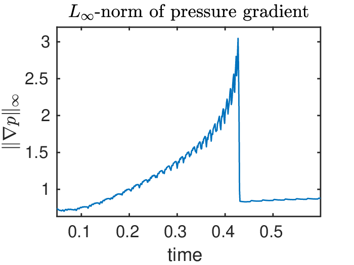
Figure 7: Focusing solution: pressure gradient norms. Plot of the pressure gradient norms along time, from the left ot the right, from the top down, L2,L4,L6,L8,L10,L∞L^{2},L^{4},L^{6},L^{8},L^{10},L^{\infty}-norm, with γ=10\gamma=10, Δ​x=0.02\Delta x=0.02, Δ​t=0.001\Delta t=0.001, pH=1p_{H}=1 and initial internal radius 0.60.6.
Refer to caption
Refer to caption
Refer to caption
Refer to caption
Refer to caption
Refer to caption
Figure 8: Focusing solution (density). Numerical solution of the focusing problem with γ=10\gamma=10, Δ​x=0.02\Delta x=0.02, initial internal radius 11.
Refer to caption
Refer to caption
Refer to caption
Refer to caption
Refer to caption
Refer to caption
Figure 9: Focusing solution (pressure). Numerical solution of the focusing problem with γ=10\gamma=10, Δ​x=0.02\Delta x=0.02, initial internal radius 11.

The Hele-Shaw problem in a spherical shell is defined by the following system

{−Δ​p∞=G⁡(p∞) in ​Ω​(t),V=−∂νp∞ on ​∂Ω⁡(t),\begin{cases}-\Delta p_{\infty}=G(p_{\infty})&\text{ in }\Omega(t),\\ \quad V\quad\,=-\partial_{\nu}p_{\infty}&\text{ on }\partial\Omega(t),\end{cases} (39)

where ν\nu and VV denote the outward normal and the normal velocity of the free boundary, with

Ω(t)={x;R1(t)≤|x|≤R2(t)}.\Omega(t)=\{x;\ R_{1}(t)\leq|x|\leq R_{2}(t)\}.

In [15] the authors compute the asymptotic behaviour of the LpL^{p}-norms in space and time of the gradient of a radial solution, choosing for the sake of simplicity a constant reaction term and external radius R2​(t)=R2R_{2}(t)=R_{2} fixed. They show that the LpL^{p}-norms are uniformly bounded (with respect to γ\gamma) if and only if p≤4p\leq 4, which confirms that the uniform L4L^{4} bound of the PME solution gradient is optimal.

We use our fully discrete scheme (19) in 2D to verify this interesting behaviour. We approximate the solution of system (39), taking γ=10\gamma=10, which is a value that well approximate the behaviour of the solution as γ→∞\gamma\rightarrow\infty.

We take as computational domain [−8,8]×[−8,8][-8,8]\times[-8,8] and G⁡(p)=1−pG(p)=1-p. The initial data is given by

n⁡(x,y)={0.8if0.6<x2+y2<6,0otherwise.n(x,y)=\begin{cases}0.8\qquad&\text{if}\quad 0.6<\sqrt{x^{2}+y^{2}}<6,\\ 0\qquad&\text{otherwise}.\end{cases} (40)

The plots of the LxqL_{x}^{q}-norms of ∇p​(t)\nabla p(t), with q=2,4,6,8q=2,4,6,8, are displayed along time in Fig. 7. We notice that at the focusing time, which is around t=0.428t=0.428, the norms with exponent larger than 44 develop a singularity. We also present 3D plots of the solution and its pressure as time evolves, cf. Fig. 8 and Fig. 9. In order to better show the behaviour and the shape of the focusing solution, we choose to take a larger initial internal radius. Hence, we take it to be equal to 1 rather than 0.6 in Eq. (40).

5 Conclusions

We studied the properties of an upwind finite difference scheme for a mechanical model of tumor growth proving stability results which allowed us to infer the asymptotic preserving property of the scheme in the so-called incompressible limit. We performed numerical simulations in order to investigate the sharpness of the L4L^{4}-uniform bound of the pressure gradient, using the focusing solution as limiting example.

The question of how to derive the Aronson-Bénilan estimate for a fixed grid and γ>1\gamma>1 remains completely open and faces several technical difficulties, due to the stronger non-linearity of the equation. Moreover, as aforementioned, it could be of use in order to pass to the limit as Δ​x→0\Delta x\rightarrow 0 in the semi-discrete scheme. Extending our approach on the Aronson-Bénilan estimate to finite difference schemes for cross-reaction-diffusion systems of porous medium type could also represent a challenging problem.

Acknowledgements

This project has received funding from the European Union’s Horizon 2020 research and innovation program under the Marie Skłodowska-Curie (grant agreement No 754362).
The authors are grateful to Benoît Perthame for many valuable discussions during the preparation of this paper.

Appendix A Proof of the solvability of (21)

The following theorem, which is a generalization of [1, Theorem A.1] holds.

Theorem A.1.

Denote n¯i​(t)\bar{n}_{i}(t) and n¯i​(t)\underline{n}_{i}(t) to be two solutions of the system of equations

d​ni​(t)d​t+(1−αi​(t))​ni​(t)−ν⁡[A⁡(ni​(t),ni+1​(t))−A⁡(ni−1​(t),ni​(t))]=Nik,i∈I,\frac{dn_{i}(t)}{dt}+(1-\alpha_{i}(t))n_{i}(t)-\nu\left[A(n_{i}(t),n_{i+1}(t))-A(n_{i-1}(t),n_{i}(t))\right]=N_{i}^{k},\quad i\in I, (41)

where A⁡(ni​(t),ni+1​(t))A(n_{i}(t),n_{i+1}(t)) is defined from (20), ν=Δ​t/Δ​x\nu=\Delta t/\Delta x, αi​(t)=Δ​t​G​(niγ​(t))\alpha_{i}(t)=\Delta tG(n_{i}^{\gamma}(t)) and Δ​t<1/G⁡(0)\Delta t<1/G(0), with a super- and a sub-solution initial data, respectively, i.e.

n¯i​(0)=pH1γ,n¯i​(0)=0.\bar{n}_{i}(0)=p_{H}^{\frac{1}{\gamma}},\quad\underline{n}_{i}(0)=0.

Then we have
(i) n¯i​(t)\bar{n}_{i}(t) and n¯i​(t)\underline{n}_{i}(t) are nonnegative for all t>0t>0 and i∈Ii\in I.
(ii) n¯i​(t)\bar{n}_{i}(t) and n¯i​(t)\underline{n}_{i}(t) are super- and sub-solutions for all t>0t>0 and i∈Ii\in I.
(iii) n¯i​(t)≥n¯i​(t)\bar{n}_{i}(t)\geq\underline{n}_{i}(t) for all t>0t>0 and i∈Ii\in I.
(iv) for any i∈Ii\in I, both n¯i​(t)\bar{n}_{i}(t) and n¯i​(t)\underline{n}_{i}(t) converges to the same limit, which is the unique solution of (21).

Proof.

(i) We prove the case of supersolution. The proof for the case of subsolution is similar. Consider the moment t∗t^{*} when n¯i​(t)\bar{n}_{i}(t) first reach 0 for some i0i_{0}, i.e. n¯i0​(t∗)=0\bar{n}_{i_{0}}(t^{*})=0 while n¯i​(t∗)≥0\bar{n}_{i}(t^{*})\geq 0 for all i≠i0i\neq i_{0}, then A⁡(n¯i0​(t),n¯i0+1​(t))≥0A(\bar{n}_{i_{0}}(t),\bar{n}_{i_{0}+1}(t))\geq 0, A⁡(n¯i0−1​(t),n¯i0​(t))≤0A(\bar{n}_{i_{0}-1}(t),\bar{n}_{i_{0}}(t))\leq 0 and thus

d​n¯i0​(t∗)d​t=ν⁡[A⁡(n¯i0​(t),n¯i0+1​(t))−A⁡(n¯i0−1​(t),n¯i0​(t))]+Ni0k≥0\frac{d\bar{n}_{i_{0}}(t^{*})}{dt}=\nu\left[A(\bar{n}_{i_{0}}(t),\bar{n}_{i_{0}+1}(t))-A(\bar{n}_{i_{0}-1}(t),\bar{n}_{i_{0}}(t))\right]+N_{i_{0}}^{k}\geq 0

via the evolution equation (41). As a result, n¯i​(t)\bar{n}_{i}(t) can’t change signs and thus remain nonnegative for all t≥0t\geq 0.

(ii) Here we prove the case of subsolution. The proof for the case of supersolution is similar. Denote

z¯i​(t)=d​n¯i​(t)d​t,α¯i​(t)=Δ​t​G​(n¯iγ​(t)),A¯i+12​(t)=A⁡(n¯i​(t),n¯i+1​(t)),\underline{z}_{i}(t)=\frac{d\underline{n}_{i}(t)}{dt},\quad\underline{\alpha}_{i}(t)=\Delta tG(\underline{n}_{i}^{\gamma}(t)),\quad\underline{A}_{i+\frac{1}{2}}(t)=A(\underline{n}_{i}(t),\underline{n}_{i+1}(t)),

then z¯i​(0)≥0\underline{z}_{i}(0)\geq 0 for all ii since n¯i​(0)\underline{n}_{i}(0) is a subsolution. Differentiating (41), we get

d​z¯i​(t)d​t+(1−α¯i​(t))​z¯i​(t)−α¯i′​(t)​n¯i​(t)−ν⁡[∂1A¯i+12−∂2A¯i−12]​z¯i​(t)\displaystyle\frac{d\underline{z}_{i}(t)}{dt}+(1-\underline{\alpha}_{i}(t))\underline{z}_{i}(t)-\underline{\alpha}_{i}^{\prime}(t)\underline{n}_{i}(t)-\nu\left[\partial_{1}\underline{A}_{i+\frac{1}{2}}-\partial_{2}\underline{A}_{i-\frac{1}{2}}\right]\underline{z}_{i}(t)
=\displaystyle= ν​∂2A¯i+12​z¯i+1​(t)−ν​∂1A¯i−12​z¯i−1​(t).\displaystyle\nu\partial_{2}\underline{A}_{i+\frac{1}{2}}\underline{z}_{i+1}(t)-\nu\partial_{1}\underline{A}_{i-\frac{1}{2}}\underline{z}_{i-1}(t).

Noticing that α¯i′​(t)=0\underline{\alpha}_{i}^{\prime}(t)=0 when z¯i​(t)=0\underline{z}_{i}(t)=0, the function z¯i​(t)\underline{z}_{i}(t) can’t change signs following a similar argument as in (i), which implies that z¯i​(t)≥0\underline{z}_{i}(t)\geq 0 for all t≥0t\geq 0. Then combining with (41), we have that

(1−α¯i​(t))​n¯i​(t)−ν⁡[A¯i+12​(t)−A¯i−12​(t)]≤Nik, for all ​t≥0,(1-\underline{\alpha}_{i}(t))\underline{n}_{i}(t)-\nu\left[\underline{A}_{i+\frac{1}{2}}(t)-\underline{A}_{i-\frac{1}{2}}(t)\right]\leq N_{i}^{k},\text{ for all }t\geq 0,

which shows that n¯i​(t)\underline{n}_{i}(t) is always a subsolution.

(iii) Denote wi​(t)=n¯i​(t)−n¯i​(t)w_{i}(t)=\bar{n}_{i}(t)-\underline{n}_{i}(t), then initially we have wi​(0)≥0w_{i}(0)\geq 0 for all ii. We wish to show that wi​(t)≥0w_{i}(t)\geq 0 for all t≥0t\geq 0 and i∈Ii\in I. For simplicity of notations, we denote

α¯i​(t)=Δ​t​G​(n¯iγ​(t)),α¯i​(t)=Δ​t​G​(n¯iγ​(t)).\bar{\alpha}_{i}(t)=\Delta tG(\bar{n}_{i}^{\gamma}(t)),\quad\underline{\alpha}_{i}(t)=\Delta tG(\underline{n}_{i}^{\gamma}(t)).

Noticing (3) and the fact that both n¯i​(t)\bar{n}_{i}(t) and n¯i​(t)\underline{n}_{i}(t) are nonnegative, when Δ​t<1/G⁡(0)\Delta t<1/G(0), we have α¯i​(t)≤1\bar{\alpha}_{i}(t)\leq 1 and α¯i​(t)≤1\underline{\alpha}_{i}(t)\leq 1. A direct computation shows that

(1−α¯i​(t))​n¯i​(t)−(1−α¯i​(t))​n¯i​(t)\displaystyle(1-\bar{\alpha}_{i}(t))\bar{n}_{i}(t)-(1-\underline{\alpha}_{i}(t))\underline{n}_{i}(t) =(1−α¯i​(t))​wi​(t)+(α¯i​(t)−α¯i​(t))​n¯i​(t)\displaystyle=(1-\bar{\alpha}_{i}(t))w_{i}(t)+(\underline{\alpha}_{i}(t)-\bar{\alpha}_{i}(t))\underline{n}_{i}(t)
=(1−α¯i​(t)+βi​(t))​wi​(t),\displaystyle=(1-\bar{\alpha}_{i}(t)+\beta_{i}(t))w_{i}(t),

where βi​(t)=−Δ​t​G′​(ηiγ​(t))​γ​ηiγ−1​(t)​n¯i​(t)≥0\beta_{i}(t)=-\Delta tG^{\prime}(\eta_{i}^{\gamma}(t))\gamma\eta_{i}^{\gamma-1}(t)\underline{n}_{i}(t)\geq 0 for some nonnegative ηi​(t)\eta_{i}(t) between n¯i​(t)\bar{n}_{i}(t) and n¯i​(t)\underline{n}_{i}(t). By (41) and the fact that n¯i​(t)\bar{n}_{i}(t) and n¯i​(t)\underline{n}_{i}(t) are super- and subsolutions, we have

(1−α¯i​(t)+βi​(t))​wi​(t)\displaystyle(1-\bar{\alpha}_{i}(t)+\beta_{i}(t))w_{i}(t) −ν⁡[Ai+12​(n¯i,n¯i+1)−Ai−12​(n¯i−1,n¯i)]\displaystyle-\nu\left[A_{i+\frac{1}{2}}(\bar{n}_{i},\bar{n}_{i+1})-A_{i-\frac{1}{2}}(\bar{n}_{i-1},\bar{n}_{i})\right]
+ν⁡[Ai+12​(n¯i,n¯i+1)−Ai−12​(n¯i−1,n¯i)]≥0.\displaystyle+\nu\left[A_{i+\frac{1}{2}}(\underline{n}_{i},\underline{n}_{i+1})-A_{i-\frac{1}{2}}(\underline{n}_{i-1},\underline{n}_{i})\right]\geq 0.

Combining the above inequality with the following expression

Ai+12​(n¯i,n¯i+1)−Ai+12​(n¯i,n¯i+1)=∂1Ai+12​(ξi,n¯i+1)​wi+∂2Ai+12​(n¯i,ηi+1)​wi+1,A_{i+\frac{1}{2}}(\bar{n}_{i},\bar{n}_{i+1})-A_{i+\frac{1}{2}}(\underline{n}_{i},\underline{n}_{i+1})=\partial_{1}A_{i+\frac{1}{2}}(\xi_{i},\bar{n}_{i+1})w_{i}+\partial_{2}A_{i+\frac{1}{2}}(\underline{n}_{i},\eta_{i+1})w_{i+1},

where ∂1Ai+12​(ξi,n¯i+1)≤0\partial_{1}A_{i+\frac{1}{2}}(\xi_{i},\bar{n}_{i+1})\leq 0 with some ξi\xi_{i} between n¯i\bar{n}_{i} and n¯i\underline{n}_{i} and ∂2Ai+12​(n¯i,ηi+1)≥0\partial_{2}A_{i+\frac{1}{2}}(\underline{n}_{i},\eta_{i+1})\geq 0 with some ηi+1\eta_{i+1} between n¯i+1\bar{n}_{i+1} and n¯i+1\underline{n}_{i+1}, we have

[1−α¯i​(t)+βi​(t)−ν⁡(∂1Ai+12​(ξi,n¯i+1)−∂2Ai−12​(n¯i−1,ηi))]​wi​(t)\displaystyle\left[1-\bar{\alpha}_{i}(t)+\beta_{i}(t)-\nu\left(\partial_{1}A_{i+\frac{1}{2}}(\xi_{i},\bar{n}_{i+1})-\partial_{2}A_{i-\frac{1}{2}}(\underline{n}_{i-1},\eta_{i})\right)\right]w_{i}(t)
−ν∂2Ai+12(n¯i,ηi+1)wi+1(t)+ν∂1Ai−12(ξi−1,n¯i)wi−1(t)≥0.\displaystyle-\nu\partial_{2}A_{i+\frac{1}{2}}(\underline{n}_{i},\eta_{i+1})w_{i+1}(t)+\nu\partial_{1}A_{i-\frac{1}{2}}(\xi_{i-1},\underline{n}_{i})w_{i-1}(t)\geq 0.

Multiplying both sides by 𝟙{wi<0}\mathds{1}_{\{w_{i}<0\}} and summing over ii, we get

−∑i(1−α¯i(t)+βi(t))wi−+I1+I2≥0,\displaystyle-\sum_{i}(1-\bar{\alpha}_{i}(t)+\beta_{i}(t))w_{i}^{-}+I_{1}+I_{2}\geq 0,

where wi−=max⁡{−wi,0}w_{i}^{-}=\max\{-w_{i},0\} and

I1=ν∑i∂2Ai−12(n¯i−1,ηi)wi(𝟙{wi<0}−𝟙{wi−1<0}),\displaystyle I_{1}=\nu\sum_{i}\partial_{2}A_{i-\frac{1}{2}}(\underline{n}_{i-1},\eta_{i})w_{i}(\mathds{1}_{\{w_{i}<0\}}-\mathds{1}_{\{w_{i-1}<0\}}),
I2=−ν∑i∂1Ai+12(ξi,n¯i+1)wi(𝟙{wi<0}−𝟙{wi+1<0}).\displaystyle I_{2}=-\nu\sum_{i}\partial_{1}A_{i+\frac{1}{2}}(\xi_{i},\underline{n}_{i+1})w_{i}(\mathds{1}_{\{w_{i}<0\}}-\mathds{1}_{\{w_{i+1}<0\}}).

It is worth noticing that

wi(𝟙{wi<0}−𝟙{wi±1<0})≤0,w_{i}(\mathds{1}_{\{w_{i}<0\}}-\mathds{1}_{\{w_{i\pm 1}<0\}})\leq 0,

which implies that I1≤0I_{1}\leq 0, I2≤0I_{2}\leq 0 and further

∑i(1−α¯i​(t)+βi​(t))​wi−≤0.\sum_{i}(1-\bar{\alpha}_{i}(t)+\beta_{i}(t))w_{i}^{-}\leq 0. (42)

It is easy to see from (42) that we must have wi−​(t)≡0w_{i}^{-}(t)\equiv 0, i.e. wi​(t)≥0w_{i}(t)\geq 0 for all t>0t>0.

(iv) The monotonicity of n¯i​(t)\bar{n}_{i}(t) and n¯i​(t)\underline{n}_{i}(t) indicates that there exist the limits

N¯i=limt→∞n¯i​(t),N¯i=limt→∞n¯i​(t).\bar{N}_{i}=\lim_{t\to\infty}\bar{n}_{i}(t),\quad\underline{N}_{i}=\lim_{t\to\infty}\underline{n}_{i}(t).

Denote Wi=N¯i−N¯iW_{i}=\bar{N}_{i}-\underline{N}_{i}, we can show that

[1−Δ​t​G​(N¯iγ)+βi​(t)−ν⁡(∂1Ai+12​(ξi,N¯i+1)−∂2Ai−12​(N¯i−1,ηi))]​Wi\displaystyle\left[1-\Delta tG(\bar{N}_{i}^{\gamma})+\beta_{i}(t)-\nu\left(\partial_{1}A_{i+\frac{1}{2}}(\xi_{i},\bar{N}_{i+1})-\partial_{2}A_{i-\frac{1}{2}}(\underline{N}_{i-1},\eta_{i})\right)\right]W_{i}
−ν∂2Ai+12(N¯i,ηi+1)Wi+1+ν∂1Ai−12(ξi−1,N¯i)Wi−1=0,\displaystyle-\nu\partial_{2}A_{i+\frac{1}{2}}(\underline{N}_{i},\eta_{i+1})W_{i+1}+\nu\partial_{1}A_{i-\frac{1}{2}}(\xi_{i-1},\underline{N}_{i})W_{i-1}=0,

for some ξi\xi_{i}’s and ηi\eta_{i}’s. Summing over all ii, we have

∑i[1−Δ​t​G​(N¯iγ)+βi​(t)]​Wi=0.\sum_{i}\left[1-\Delta tG(\bar{N}_{i}^{\gamma})+\beta_{i}(t)\right]W_{i}=0.

Noticing that Wi≥0W_{i}\geq 0 and 1−Δ​t​G​(N¯iγ)+βi​(t)>01-\Delta tG(\bar{N}_{i}^{\gamma})+\beta_{i}(t)>0, we have Wi=0W_{i}=0 for all i∈Ii\in I. In other words, for each ii, there is a unique limit of n¯i​(t)\bar{n}_{i}(t) and n¯i​(t)\underline{n}_{i}(t) as t→∞t\to\infty, which is Nik+1N_{i}^{k+1}, the unique solution of (21).

∎

References

  • [1] L. Almeida, F. Bubba, B. Perthame, and C. Pouchol. Energy and implicit discretization of the fokker-planck and keller-segel type equations. Networks & Heterogeneous Media, 14:23–41, 2019.
  • [2] D. G. Aronson. The focusing problem for the porous medium equation: Experiment, simulation and analysis. Nonlinear Analysis, 137:135 – 147, 2016. Nonlinear Partial Differential Equations, in honor of Juan Luis Vázquez for his 70th birthday.
  • [3] D. G. Aronson, O. Gil, and J. L. Vázquez. Limit behaviour of focusing solutions to nonlinear diffusions. Comm. Partial Differential Equations, 23(1-2):307–332, 1998.
  • [4] D. G. Aronson and J. L. Graveleau. A selfsimilar solution to the focusing problem for the porous medium equation. European Journal of Applied Mathematics, 4(1):65–81, 1993.
  • [5] M. J. Baines, M. E. Hubbard, and P. K. Jimack. A moving mesh finite element algorithm for the adaptive solution of time-dependent partial differential equations with moving boundaries. Appl. Numer. Math., 54:450–469, 2005.
  • [6] M. J. Baines, M. E. Hubbard, P. K. Jimack, and A. C. Jones. Scale-invariant moving finite elements for nonlinear partial differential equations in two dimensions. Appl. Numer. Math., 56:230–252, 2006.
  • [7] E. D. Benedetto and D. Hoff. An interface tracking algorithm for the porous medium equation. Transactions of the American Mathematical Society, 284:463–500, 1984.
  • [8] M. Bessemoulin-Chatard and F. Filbet. A finite volume scheme for nonlinear degenerate parabolic equations. SIAM J. Sci. Comput., 34:B559–B583, 2012.
  • [9] F. Bubba, B. Perthame, C. Pouchol, and M. Schmidtchen. Hele-Shaw limit for a system of two reaction-(cross-)diffusion equations for living tissues. Arch. Rational. Mech. Anal., 236:735–766, 2020.
  • [10] C. J. Budd, G. J. Collins, W. Z. Huang, and R. D. Russell. Self–similar numerical solutions of the porous–medium equation using moving mesh methods. Philos. T. Roy. Soc. A., 357:1047–1077, 1999.
  • [11] J. A. Carrillo, B. Düring, D. Matthes, and D. McCormick. A lagrangian scheme for the solution of nonlinear diffusion equations using moving simplex meshes. J. Sci. Comp., 75:463–1499, 2018.
  • [12] J. A. Carrillo, Y. Huang, F. S. Patacchini, and G. Wolansky. Numerical study of a particle method for gradient flows. Kinet. Relat. Mod., 10, 2017.
  • [13] J. A. Carrillo, H. Ranetbauer, and M.-T. Wolfram. Numerical simulation of nonlinear continuity equations by evolving diffeomorphisms. J. Comp. Phys., 327:186–202, 2016.
  • [14] F. Cavalli, G. Naldi, G. Puppo, and M. Semplice. High-order relaxation schemes for nonlinear degenerate diffusion problems. SIAM J. Numer. Analy., 45, 2007.
  • [15] N. David and B. Perthame. Free boundary limit of a tumor growth model with nutrient. Journal de Mathématiques Pures et Appliquées, 2021.
  • [16] T. Dębiec, B. Perthame, M. Schmidtchen, and N. Vauchelet. Incompressible limit for a two-species model with coupling through Brinkman’s law in any dimension. Journal de Mathématiques Pures et Appliquées, 145:204–239, 2021.
  • [17] P. Degond, S. Hecht, and N. Vauchelet. Incompressible limit of a continuum model of tissue growth for two cell populations. Networks & Heterogeneous Media, 15(1):57–85, 2020.
  • [18] R. Eymard, T. Gallout, R. Herbin, and A. Michel. Convergence of a finite volume scheme for nonlinear degenerate parabolic equations. Numer. Math., 92:41–82, 2002.
  • [19] J. L. Graveleau and P. Jamet. A finite difference approach to some degenerate nonlinear parabolic equation. SIAM J. Appl. Math., 20:199–223, 1971.
  • [20] S. Jin and Z. P. Xin. Commu. Pure Appl. Math., 48:235–277, 1995.
  • [21] I. Kim and N. Požár. Porous medium equation to Hele-Shaw flow with general initial density. Trans. Amer. Math. Soc., 370(2):873–909, 2018.
  • [22] C. Liu and Y. Wang. On lagrangian schemes for porous medium type generalized diffusion equations: A discrete energetic variational approach. J. Comp. Phys, 417:109566, 2020.
  • [23] J.-G. Liu, M. Tang, L. Wang, and Z. Zhou. An accurate front capturing scheme for tumor growth models with a free boundary limit. Journal of Computational Physics, 364:73–94, 2018.
  • [24] J.-G. Liu, M. Tang, L. Wang, and Z. Zhou. Analysis and computation of some tumor growth models with nutrient: From cell density models to free boundary dynamics. Discrete & Continuous Dynamical Systems - B, 24:3011, 2019.
  • [25] Y. Liu, C.-W. Shu, and M. Zhang. High order finite difference weno schemes for nonlinear degenerate parabolic equations. SIAM J. Sci. Comp., 33:939–965, 2011.
  • [26] P. Macklin, S. McDougall, A. R. A. Anderson, M. A. J. Chaplain, V. Cristini, and J. Lowengrub. Multiscale modelling and nonlinear simulation of vascular tumour growth. Journal of Mathematical Biology, 58(4):765–798, 2009.
  • [27] L. Monsaingeon. An explicit finite-difference scheme for one-dimensional generalized porous medium equations: Interface tracking and the hole filling problem. ESAIM: M2AN, 50(4):1011–1033, 2016.
  • [28] G. Naldi, L. Pareschi, and G. Toscani. Relaxation schemes for partial differential equations and applications to degenerate diffusion problems. Surv. Math. Ind., 10:315–343, 2002.
  • [29] C. Ngo and W. Huang. A study on moving mesh finite element solution of the porous medium equation. J. Comp. Phys., 331:357–380, 2017.
  • [30] B. Perthame, F. Quirós, and J. L. Vázquez. The Hele-Shaw asymptotics for mechanical models of tumor growth. Arch. Ration. Mech. Anal., 212(1):93–127, 2014.
  • [31] B. Perthame, F. Quirós, M. Tang, and N. Vauchelet. Derivation of a Hele-Shaw type system from a cell model with active motion. Interfaces Free Bound., 16(4):489–508, 2014.
  • [32] B. Perthame, M. Tang, and N. Vauchelet. Traveling wave solution of the Hele-Shaw model of tumor growth with nutrient. Math. Models Methods Appl. Sci., 24(13):2601–2626, 2014.
  • [33] B. Perthame and N. Vauchelet. Incompressible limit of a mechanical model of tumour growth with viscosity. Philos. Trans. Roy. Soc. A, 373(2050):20140283, 16, 2015.
  • [34] M. E. Rose. Numerical methods for flows through porous media. i. Math. Comp., 40:435–467, 1983.
  • [35] Q. Zhang and Z.-L. Wu. Numerical simulation for porous medium equation by local discontinuous galerkin finite element method. J. Sci. Comp., 38:127–148, 2009.