跳到论文正文
W Papers独立论文阅读器 arXiv:2105.10253 论文正文 计算阅读时间 · 0%
引用这篇论文根据当前论文元数据生成,正式投稿前建议核对。


License: arXiv.org perpetual non-exclusive license
arXiv:2105.10253v1 [math.AP] 21 May 2021

Elastic anisotropy of nematic liquid crystals in the two-dimensional Landau-de Gennes model

Yucen Han1 Affiliation: 1 Department of Mathematics and Statistics, University of Strathclyde, G1 1XQ, United Kindom.
2Beijing International Center for Mathematical Research, Center for Quantitative Biology, Peking University, Beijing 100871, China.
   Joseph Harris1 Affiliation: 1 Department of Mathematics and Statistics, University of Strathclyde, G1 1XQ, United Kindom.
2Beijing International Center for Mathematical Research, Center for Quantitative Biology, Peking University, Beijing 100871, China.
   Lei Zhang2 Affiliation: 1 Department of Mathematics and Statistics, University of Strathclyde, G1 1XQ, United Kindom.
2Beijing International Center for Mathematical Research, Center for Quantitative Biology, Peking University, Beijing 100871, China.
   Apala Majumdar1 Affiliation: 1 Department of Mathematics and Statistics, University of Strathclyde, G1 1XQ, United Kindom.
2Beijing International Center for Mathematical Research, Center for Quantitative Biology, Peking University, Beijing 100871, China.
Abstract

We study the effects of elastic anisotropy on the Landau-de Gennes critical points for nematic liquid crystals, in a square domain. The elastic anisotropy is captured by a parameter, L2L_{2}, and the critical points are described by three degrees of freedom. We analytically construct a symmetric critical point for all admissible values of L2L_{2}, which is necessarily globally stable for small domains i.e., when the square edge length, λ\lambda, is small enough. We perform asymptotic analyses and numerical studies to discover at least 55 classes of these symmetric critical points - the W​O​R​SWORS, R​i​n​g±Ring^{\pm}, C​o​n​s​t​a​n​tConstant and p​W​O​R​SpWORS solutions, of which the W​O​R​SWORS, R​i​n​g+Ring^{+} and C​o​n​s​t​a​n​tConstant solutions can be stable. Furthermore, we demonstrate that the novel C​o​n​s​t​a​n​tConstant solution is energetically preferable for large λ\lambda and large L2L_{2}, and prove associated stability results that corroborate the stabilising effects of L2L_{2} for reduced Landau-de Gennes critical points. We complement our analysis with numerically computed bifurcation diagrams for different values of L2L_{2}, which illustrate the interplay of elastic anisotropy and geometry for nematic solution landscapes, at low temperatures.

I Introduction

Nematic liquid crystals (NLCs) are quintessential examples of partially ordered materials that combine fluidity with the directionality of solids prost1995physics. The nematic molecules are typically asymmetric in shape e.g., rod- or disc-shaped, and these molecules tend to align along certain locally preferred averaged directions, referred to as nematic directors in the literature. Consequently, NLCs have a degree of long-range orientational order and direction-dependent physical, optical and rheological properties. It is precisely this anisotropy that makes them the working material of choice for a range of electro-optic devices such as the multi-billion dollar liquid crystal display industry lagerwallreview; wang2021modeling.

There has been substantial recent interest in multistable NLC systems i.e., NLCs, confined to two-dimensional (2D), or three-dimensional (3D) geometries that can support multiple stable states without any external electric fields robinson2017molecular; kusumaatmaja2015free; luo2012multistability; canevari2017order; canevariharrismajumdarwang; han2019transition; yin2020construction. Multistable NLC systems offer new prospects for device technologies, materials technologies, self-assembly processes and hydrodynamics. This paper is motivated by a bistable system reported in tsakonas2007multistable. Here, the authors experimentally and numerically study NLCs inside periodic arrays of 3D wells, with a square cross-section, such that the well height is typically much smaller than the square cross-sectional length. Furthermore, the authors speculate that the structural characteristics only vary in the plane of the square cross-section, and are translationally invariant along the well-height, effectively reducing this to a 2D problem. Hence, the authors restrict attention to the bottom square cross-section of the well geometry, where the square edge length is denoted by λ\lambda and is typically on the micron scale. The choice of boundary conditions is crucial for any confined NLC system and, in tsakonas2007multistable, the authors impose tangent boundary conditions (TBCs) on the well surfaces i.e., the nematic directors, in the plane of the well surfaces, are constrained to be tangent to those well surfaces. However, this necessarily means that the nematic director has to be tangent to the square edges, creating defects at the vertices where the director is not defined. The authors observe two classes of stable NLC states in this geometry: the diagonal DD states, for which the nematic director aligns along one of the square diagonals and; the rotated RR states, for which the director rotates by π\pi radians between a pair of opposite square edges.

In kralj2014order, luo2012multistability, the authors model this square system within the celebrated continuum Landau-de Gennes (LdG) theory for NLCs. The LdG theory describes the state of nematic anisotropy by a macroscopic order parameter - the 𝐐\mathbf{Q}-tensor order parameter prost1995physics. From an experimental perspective, the 𝐐\mathbf{Q}-tensor is measured in terms of NLC responses to external electric or magnetic fields, which are necessarily anisotropic in nature. Mathematically, the 𝐐\mathbf{Q}-tensor order parameter is a symmetric, traceless, 3×33\times 3 matrix whose eigenvectors represent the special directions of preferred molecular alignment, and the corresponding eigenvalues measure the degree of orientational order about these directions; more details are given in the next section. The nematic director can be identified with the eigenvector that has the largest positive eigenvalue. For a square domain with TBCs on the square edges, it suffices to work in a reduced LdG framework where the 𝐐\mathbf{Q}-tensor only has three degrees of freedom, q1,q2,q3q_{1},q_{2},q_{3}. The degree of nematic order in the plane is captured by q1q_{1} and q2q_{2}, whereas q3q_{3} measures the out-of-plane order, such that positive (negative) q3q_{3} implies that the nematic director lies out of the plane (in the plane) of the square, respectively. The TBCs naturally constrain q3q_{3} to be negative on the square edges, but q3q_{3} could be positive in the interior, away from the square edges, for energetic reasons. The LdG theory is a variational theory i.e., experimentally observable states can be modelled by local or global minimizers of an appropriately defined LdG free energy. In the simplest setting, the LdG energy has two contributions - a bulk energy that only depends on the eigenvalues of the 𝐐\mathbf{Q}-tensor, and an elastic energy that penalises spatial inhomogeneities of the 𝐐\mathbf{Q}-tensor. In these papers, the authors work with low temperatures that favour an ordered nematic state for a spatially homogeneous system i.e., the bulk energy attains its minimum at an ordered nematic state for low temperatures, and attains its minimum at a disordered isotropic phase for high temperatures. The elastic energy is typically a quadratic and convex function of ∇𝐐\nabla\mathbf{Q} and, in kralj2014order, luo2012multistability, the authors work with an isotropic elastic energy - the Dirichlet elastic energy. In a reduced LdG setting, the authors recover the stable DD and RR states for large λ\lambda and, in kralj2014order, they discover a novel stable Well Order Reconstruction Solution (W​O​R​SWORS) for small λ\lambda. The W​O​R​SWORS is special because it exhibits a pair of mutually orthogonal defect lines, with no planar nematic order, along the square diagonals as will be described in Section III. In han2020pol, the authors generalise this work to arbitrary 2D regular polygons and, in canevariharrismajumdarwang, the authors study 3D wells, with an emphasis on novel mixed solutions which interpolate between two distinct DD solutions on the top and bottom well surfaces.

In this paper, we study the same problem of NLCs on a square domain with TBCs on the square edges, with an anisotropic elastic energy as opposed to the isotropic energy studied in kralj2014order and luo2012multistability. Notably, we take the elastic energy density to be w⁡(∇𝐐)=|∇𝐐|2+L2​(div​𝐐)2w(\nabla\mathbf{Q})=|\nabla\mathbf{Q}|^{2}+L_{2}\left(\textrm{div}\mathbf{Q}\right)^{2}, where −1<L2-1<L_{2} is the anisotropy parameter. Physically speaking, positive L2L_{2} implies that splay and twist deformations of the nematic director are energetically expensive compared to out-of-plane twist deformations i.e., we would expect the physically observable states to have positive q3q_{3} in the square interior as L2L_{2} increases. Therefore, we would expect to see competing effects of the TBCs on the square edges, which prefer in-plane director orientation, and the preferred out-of-plane director orientation in the square interior, for larger values of L2L_{2}. We construct a critical point of the LdG energy, for any L2>−1L_{2}>-1, for which q1=0q_{1}=0 on the square diagonals and q2=0q_{2}=0 on the coordinate axes such that the axes are parallel to the square edges. This symmetric critical point is globally stable for λ\lambda small enough. The W​O​R​SWORS is a special case of this symmetric critical point with q2≡0q_{2}\equiv 0 on the square domain, for L2=0L_{2}=0. For L2≠0L_{2}\neq 0, this class of symmetric critical points cannot have q2q_{2} identically zero on the domain, and this destroys the perfect cross symmetry of the W​O​R​SWORS. We perform an asymptotic analysis for small λ\lambda and small L2L_{2}, about the W​O​R​SWORS, which is the globally stable branch in this regime for L2=0L_{2}=0. The anisotropy has a first order effect on q3q_{3} i.e., q3q_{3} is perturbed linearly by L2L_{2}, whereas q1q_{1} and q2q_{2} exhibit quadratic perturbations. We show that q3q_{3} increases at the square centre for positive L2L_{2}, relative to its value for L2=0L_{2}=0, corroborating the trend of increasing q3q_{3} with increasing L2L_{2}. The globally stable symmetric critical point for small λ\lambda and small L2L_{2}, labelled as the R​i​n​g+Ring^{+} solution, effectively smoothens out the W​O​R​SWORS and exhibits a stable central +1+1-degree point defect. We perform formal calculations to show that as L2→∞L_{2}\to\infty, energy minimizers (and consequently the symmetric critical point described above for small λ\lambda) approach the C​o​n​s​t​a​n​tConstant state with (q1,q2,q3)=(0,0,s+/3)(q_{1},q_{2},q_{3})=(0,0,s_{+}/3) away from the square edges. The special choice of q3=s+/3q_{3}=s_{+}/3 stems from energy minimality and the choice of TBCs on the square edges. Thus, there are three different classes of the symmetric critical point discussed above: the W​O​R​SWORS, which only exists for L2=0L_{2}=0; the R​i​n​g+Ring^{+} solution, which only ceases to exist for L2L_{2} large enough, and can be stable for moderate values of λ\lambda and non-zero L2L_{2} and; the C​o​n​s​t​a​n​tConstant solution, which exists for L2L_{2} large enough and is always stable according to our heuristics and numerical calculations. Additionally, we also find two unstable classes of this symmetric critical point, both of which exist for moderate values of λ\lambda and L2L_{2}. These are the R​i​n​g−Ring^{-} solution which exhibits a central −1-1-degree point defect, and the novel p​W​O​R​SpWORS which exhibits an oscillating sequence of nematic point defects along the square diagonals. We provide asymptotic approximations for the novel p​W​O​R​SpWORS solution branch.

Whilst most of our work is restricted to the small λ\lambda-limit, we also provide rigorous results for energy minimizers in the λ→∞\lambda\to\infty limit. The competitors in the large λ\lambda-limit are the familiar DD and RR states, and the C​o​n​s​t​a​n​tConstant solution. Using Gamma-convergence arguments, we show that the C​o​n​s​t​a​n​tConstant solution has lower energy than the DD and RR states, for large enough L2L_{2}. We complement our analysis with numerical computations of bifurcation diagrams for five different values of L2L_{2}. As L2L_{2} increases, we observe that the unique minimizer for small λ\lambda changes from the W​O​R​SWORS (L2=0L_{2}=0), to the R​i​n​g+Ring^{+} and then to the C​o​n​s​t​a​n​tConstant solution. As L2L_{2} increases further, the R​i​n​g+Ring^{+} and C​o​n​s​t​a​n​tConstant solutions retain stability in the reduced framework, over an increasing range of λ\lambda. We further prove this by performing an analysis of the corresponding second variation of the reduced LdG energy. It is interesting to note that whilst the W​O​R​SWORS and R​i​n​g+Ring^{+} solution branches are connected to the DD and RR states, the C​o​n​s​t​a​n​tConstant solution branch appears to be disconnected from the DD and RR solution branches. Our notable findings concern the response of the NLC solution landscape for this model problem, to the elastic anisotropy L2L_{2}. We report (i) novel stable states (R​i​n​g+Ring^{+} and C​o​n​s​t​a​n​tConstant) for small λ\lambda, and (ii) enhanced multistability in the large λ\lambda-limit due to the competing C​o​n​s​t​a​n​tConstant and R​i​n​g+Ring^{+} states, for large L2L_{2}. As L2L_{2} increases, we expect that there are further, not necessarily energy-minimizing, LdG critical points with positive q3q_{3}, or out-of-plane nematic directors. Furthermore, L2L_{2} has a stabilising effect with respect to certain classes of perturbations: planar perturbations and out-of-plane perturbations, and so we expect enhanced multistability as L2L_{2} increases, for all values of λ\lambda.

A lot of open questions remain with regards to the interplay between L2L_{2}, λ\lambda and temperature on NLC solution landscapes, but our work is an informative forward step in this direction. Our paper is organised as follows. We provide all the mathematical preliminaries in Section II. We construct the symmetric critical points described above and prove their global stability for small λ\lambda in Section III. In Section IV, we perform separate asymptotic studies in the small λ\lambda and small L2L_{2} limit; large L2L_{2} limit; large λ\lambda-limit. In Section V, we present bifurcation diagrams for the solution landscapes with five different values of L2L_{2}, accompanied by some rigorous stability results. We conclude with some perspectives in Section VI.

II Preliminaries

In this section, we review the Landau-de Gennes (LdG) continuum theory of nematic liquid crystals. Within this framework, the nematic state is described by a macroscopic LdG order parameter - the 𝐐\mathbf{Q}-tensor order parameter. The 𝐐\mathbf{Q}-tensor is a symmetric, traceless, 3×33\times 3 matrix, which is a macroscopic measure of the nematic anisotropy. The eigenvectors of 𝐐\mathbf{Q} represent the averaged directions of preferred molecular alignment and the corresponding eigenvalues measure the degree of order about these eigen-directions. The 𝐐\mathbf{Q}-tensor is said to be: (i) isotropic if 𝐐=0\mathbf{Q}=0; (ii) uniaxial if 𝐐\mathbf{Q} has a pair of degenerate non-zero eigenvalues; and (iii) biaxial if 𝐐\mathbf{Q} has three distinct eigenvalues. A uniaxial 𝐐\mathbf{Q}-tensor can be written as 𝐐u=s⁡(𝐧⊗𝐧−𝐈/3)\mathbf{Q}_{u}=s\left(\mathbf{n}\otimes\mathbf{n}-\mathbf{I}/3\right), where 𝐈\mathbf{I} is the 3×33\times 3 identity matrix, 𝐧∈S2\mathbf{n}\in S^{2} is the distinguished eigenvector with the non-degenerate eigenvalue, and s∈ℝs\in\mathbb{R} is a scalar order parameter that measures the degree of orientational order about 𝐧\mathbf{n}. The unit vector, 𝐧\mathbf{n}, is referred to as the “director”, and physically denotes the single distinguished direction of uniaxial nematic alignment Virga94, prost1995physics. The LdG theory is a variational theory, and hence, has an associated free energy, and the basic modelling hypothesis is that the physically observable configurations correspond to global or local energy minimizers subject to imposed boundary conditions. We work with two-dimensional (2D) domains, Ω⊂ℝ2\Omega\subset\mathbb{R}^{2}, in the context of modelling thin three-dimensional (3D) systems. In the absence of a surface anchoring energy and external electric/magnetic fields, the LdG free energy is given by

ℱ⁡[𝐐]:=∫Ωfe​l​(𝐐,∇𝐐)+fb​(𝐐)​dA,\displaystyle\mathcal{F}[\mathbf{Q}]:=\int_{\Omega}f_{el}(\mathbf{Q},\nabla\mathbf{Q})+f_{b}(\mathbf{Q})\,\mathrm{dA}, (2.1)

where fe​lf_{el} and fbf_{b} are the elastic and thermotropic bulk energy densities, respectively. We consider a two-term elastic energy density given by

fe​l​(𝐐)=L2​(|∇𝐐|2+L2​(div​𝐐)2),\displaystyle f_{el}(\mathbf{Q})=\frac{L}{2}\left(|\nabla\mathbf{Q}|^{2}+L_{2}(\mathrm{div}{\mathbf{Q}})^{2}\right), (2.2)

where L>0L>0 is an elastic constant, and L2∈(−1,∞)L_{2}\in(-1,\infty) is the “elastic anisotropy” parameter. The elastic energy density penalises spatial inhomogeneities, typically quadratic in ∇𝐐\nabla\mathbf{Q}. In terms of notation, we use |∇𝐐|2:=∂Qi​j∂xk​∂Qi​j∂xk|\nabla\mathbf{Q}|^{2}:=\frac{\partial Q_{ij}}{\partial x_{k}}\frac{\partial Q_{ij}}{\partial x_{k}} and (div​𝐐)2:=∂Qi​j∂xj​∂Qi​k∂xk(\mathrm{div}{\mathbf{Q}})^{2}:=\frac{\partial Q_{ij}}{\partial x_{j}}\frac{\partial Q_{ik}}{\partial x_{k}}, i,j,k=1,2,3,i,j,k=1,2,3, where the Einstein summation convention is assumed throughout this manuscript. Since in this work we assume a 2D confining geometry Ω\Omega, we have that ∂Qi​j∂x3=0\frac{\partial Q_{ij}}{\partial x_{3}}=0 for all 1≤i,j≤31\leq i,j\leq 3. We work with the simplest form of fbf_{b}, that allows for a first-order isotropic-nematic transition as a function of the temperature:

fb​(𝐐):=A2​tr​𝐐2−B3​tr​𝐐3+C4​(tr​𝐐2)2.\displaystyle f_{b}(\mathbf{Q}):=\frac{A}{2}\mathrm{tr}\mathbf{Q}^{2}-\frac{B}{3}\mathrm{tr}\mathbf{Q}^{3}+\frac{C}{4}(\mathrm{tr}\mathbf{Q}^{2})^{2}. (2.3)

Here, tr​𝐐2=Qi​j​Qi​j\mathrm{tr}\mathbf{Q}^{2}=Q_{ij}Q_{ij}, and tr​𝐐3=Qi​j​Qj​k​Qk​i\mathrm{tr}\mathbf{Q}^{3}=Q_{ij}Q_{jk}Q_{ki}, for i,j,k=1,2,3i,j,k=1,2,3. We take A=α⁡(T−T∗)A=\alpha(T-T^{*}) to be the rescaled temperature and α,B,C>0\alpha,B,C>0 are material-dependent constants. In this regime, TT is the absolute temperature in the system, and T∗T^{*} is the characteristic nematic supercooling temperature. The rescaled temperature, AA, has three physically relevant values: (i) A=0A=0, below which the isotropic state 𝐐=0\mathbf{Q}=0 loses stability; (ii) the nematic super-heating temperature A=B2/24​CA=B^{2}/24C, above which the isotropic state is the unique critical point of fbf_{b}; and (iii) the nematic-isotropic phase transition temperature A=B2/27​CA=B^{2}/27C, at which fbf_{b} is minimized by the isotropic phase and a continuum of uniaxial states. We work with low temperatures, A<0A<0, for which fbf_{b} is minimized on the set of uniaxial 𝐐\mathbf{Q}-tensors defined by 𝒩:={𝐐∈S0:𝐐=s+​(𝐧⊗𝐧−𝐈/3)}\mathcal{N}:=\{\mathbf{Q}\in S_{0}:\mathbf{Q}=s_{+}(\mathbf{n}\otimes\mathbf{n}-\mathbf{I}/3)\} where S0S_{0} is the space of traceless symmetric 3×33\times 3 matrices and

s+=B+B2+24​|A|​C4​C,𝐧∈S2​arbitrary.\displaystyle s_{+}=\frac{B+\sqrt{B^{2}+24|A|C}}{4C},\quad\mathbf{n}\in S^{2}\,\,\text{arbitrary}. (2.4)

We non-dimensionalize the system using a change of variables, 𝐱¯=𝐱/λ\mathbf{\bar{x}}=\mathbf{x}/\lambda, where λ\lambda is a characteristic geometrical length-scale e.g., edge length of a 2D regular polygon. The rescaled LdG energy functional (upto a multiplicative constant) is given by:

ℱλ​[𝐐]:=∫Ω¯{12​|∇𝐱¯𝐐|2+L22​(div𝐱¯​𝐐)2+λ2L​fb​(𝐐)}​𝑑A¯,\displaystyle\mathcal{F}_{\lambda}[\mathbf{Q}]:=\int_{\bar{\Omega}}\left\{\frac{1}{2}|\nabla_{\mathbf{\bar{x}}}\mathbf{Q}|^{2}+\frac{L_{2}}{2}(\mathrm{div}_{\mathbf{\bar{x}}}\mathbf{Q})^{2}+\frac{\lambda^{2}}{L}f_{b}(\mathbf{Q})\right\}\,\mathrm{d\bar{A}}, (2.5)

where Ω¯\bar{\Omega} is the rescaled domain in ℝ2\mathbb{R}^{2}, and d​A¯\mathrm{d\bar{A}} is the rescaled area element. We drop the ‘bars’ but all computations should be interpreted in terms of the rescaled variables.

Next, we define the working domain and Dirichlet boundary conditions for the purposes of this paper, although we believe that our methods can be generalised to arbitrary 2D domains, and other types of Dirichlet conditions. We focus on square domains, building on the substantial work in Walton2018, canevari2017order, wang2019order. We impose Dirichlet tangent boundary conditions (TBCs) on the square edges, which require the nematic director to be tangent to the edges, necessarily creating a mismatch at the square vertices. To avoid the discontinuities at the vertices, we take Ω⊂ℝ2\Omega\subset\mathbb{R}^{2} to be a truncated square whose edges are parallel to the coordinate axes:

Ω:={(x,y)∈ℝ2:|x|<1,|y|<1,|x+y|<2−ϵ,|x−y|<2−ϵ}.\displaystyle\Omega:=\{(x,y)\in\mathbb{R}^{2}:|x|<1,|y|<1,|x+y|<2-\epsilon,|x-y|<2-\epsilon\}. (2.6)

Provided ϵ≪1\epsilon\ll 1, the truncation does not change the qualitative properties of the LdG energy minimizers away from the square vertices. The boundary, ∂Ω\partial\Omega, has four “long” edges parallel to the coordinate axes which we define in a clockwise fashion as C1,…,C4C_{1},\dots,C_{4}, where C1C_{1} lies parallel to the xx-axis at y=1y=1. The truncation creates four additional “short” edges, of length 2​ϵ\sqrt{2}\epsilon, parallel to the lines y=xy=x and y=−xy=-x, which we label as S1,…,S4S_{1},\dots,S_{4} in a clockwise fashion, starting at the top-left corner of the domain. The domain is illustrated in Figure 2.1.

Figure 2.1: The truncated square domain Ω\Omega.

We impose tangent uniaxial Dirichlet conditions on the long edges, consistent with the experimentally and numerically investigated TBCs, tsakonas2007multistable, luo2012multistability and kralj2014order. In particular, we fix 𝐧=(±1,0)\mathbf{n}=\left(\pm 1,0\right) on the edges, C1C_{1} and C3C_{3}, and 𝐧=(0,±1)\mathbf{n}=\left(0,\pm 1\right) on C2C_{2} and C4C_{4}. From a physical standpoint, this constitutes strong (infinite) anchoring on the long edges. One could also model weak (finite) anchoring condition with an additional surface energy in the LdG free energy newtonmottram, but that would make the analysis more complicated for the time being. We set

𝐐=𝐐bon∂Ω,\displaystyle\mathbf{Q}=\mathbf{Q}_{b}\qquad\text{on}\qquad\partial\Omega, (2.7)

where

𝐐b​(x,y):={s+(𝐱^⊗𝐱^−𝐈/3),(x,y)∈C1∪C3,s+(𝐲^⊗𝐲^−𝐈/3),(x,y)∈C2∪C4,\displaystyle\mathbf{Q}_{b}(x,y):=\begin{cases}s_{+}\left(\hat{\mathbf{x}}\otimes\hat{\mathbf{x}}-\mathbf{I}/3\right),\qquad&(x,y)\in C_{1}\cup C_{3},\\ s_{+}\left(\hat{\mathbf{y}}\otimes\hat{\mathbf{y}}-\mathbf{I}/3\right),\qquad&(x,y)\in C_{2}\cup C_{4},\end{cases} (2.8)

where 𝐱^\hat{\mathbf{x}} and 𝐲^\hat{\mathbf{y}} are unit vectors in the xx- and yy-direction, respectively. In particular, 𝐐b∈𝒩\mathbf{Q}_{b}\in\mathcal{N} on C1,…,C4C_{1},\ldots,C_{4}. On the short edges, S1,…,S4S_{1},\dots,S_{4}, we effectively prescribe a continuous interpolation between the boundary conditions on the associated long edges (2.8) given by:

𝐐b​(x,y):={g(x+y)(𝐱^⊗𝐱^−𝐲^⊗𝐲^)−s+2(𝐳^⊗𝐳^−𝐈/3),(x,y)∈S1,g(y−x)(𝐱^⊗𝐱^−𝐲^⊗𝐲^)−s+2(𝐳^⊗𝐳^−𝐈/3),(x,y)∈S2,g(−x−y)(𝐱^⊗𝐱^−𝐲^⊗𝐲^)−s+2(𝐳^⊗𝐳^−𝐈/3),(x,y)∈S3,g(x−y)(𝐱^⊗𝐱^−𝐲^⊗𝐲^)−s+2(𝐳^⊗𝐳^−𝐈/3),(x,y)∈S4,\displaystyle\mathbf{Q}_{b}(x,y):=\begin{cases}g(x+y)(\hat{\mathbf{x}}\otimes\hat{\mathbf{x}}-\hat{\mathbf{y}}\otimes\hat{\mathbf{y}})-\frac{s_{+}}{2}(\hat{\mathbf{z}}\otimes\hat{\mathbf{z}}-\mathbf{I}/3),\quad&(x,y)\in S_{1},\\ g(y-x)(\hat{\mathbf{x}}\otimes\hat{\mathbf{x}}-\hat{\mathbf{y}}\otimes\hat{\mathbf{y}})-\frac{s_{+}}{2}(\hat{\mathbf{z}}\otimes\hat{\mathbf{z}}-\mathbf{I}/3),\quad&(x,y)\in S_{2},\\ g(-x-y)(\hat{\mathbf{x}}\otimes\hat{\mathbf{x}}-\hat{\mathbf{y}}\otimes\hat{\mathbf{y}})-\frac{s_{+}}{2}(\hat{\mathbf{z}}\otimes\hat{\mathbf{z}}-\mathbf{I}/3),\quad&(x,y)\in S_{3},\\ g(x-y)(\hat{\mathbf{x}}\otimes\hat{\mathbf{x}}-\hat{\mathbf{y}}\otimes\hat{\mathbf{y}})-\frac{s_{+}}{2}(\hat{\mathbf{z}}\otimes\hat{\mathbf{z}}-\mathbf{I}/3),\quad&(x,y)\in S_{4},\end{cases} (2.9)

where 𝐳^\hat{\mathbf{z}} is a unit vector in the zz-direction, and g:[−ϵ,ϵ]→[−s+/2,s+/2]g:[-\epsilon,\epsilon]\to[-s_{+}/2,s_{+}/2] is a smoothing function defined as

g⁡(l)=s+2​ϵ​l,−ϵ≤l≤ϵ.\displaystyle g(l)=\frac{s_{+}}{2\epsilon}l,\qquad-\epsilon\leq l\leq\epsilon. (2.10)

Although the boundary conditions (2.9) do not minimize fbf_{b} on S1,…,S4S_{1},\dots,S_{4}, and do not respect TBCs, they are short by construction and are chosen purely for mathematical convenience. Given the Dirichlet boundary conditions (2.8) and (2.9), we define our admissible space to be

𝒜:={𝐐∈W1,2​(Ω,S0):𝐐=𝐐b​on​∂Ω}.\displaystyle\mathcal{A}:=\{\mathbf{Q}\in W^{1,2}(\Omega;S_{0}):\mathbf{Q}=\mathbf{Q}_{b}\,\,\,\,\text{on}\,\,\,\partial\Omega\}. (2.11)

The energy minimizers, or indeed any critical point of the LdG energy (2.5), are solutions of the associated Euler-Lagrange equations:

Δ​Qi​j+L22​(Qi​k,k​j+Qj​k,k​i−23​δi​j​Qk​l,k​l)=λ2L​{A​Qi​j−B⁡(Qi​k​Qk​j−13​δi​j​tr​𝐐2)+C​Qi​j​tr​𝐐2},\displaystyle\Delta Q_{ij}+\frac{L_{2}}{2}\left(Q_{ik,kj}+Q_{jk,ki}-\frac{2}{3}\delta_{ij}Q_{kl,kl}\right)=\frac{\lambda^{2}}{L}\left\{AQ_{ij}-B\left(Q_{ik}Q_{kj}-\frac{1}{3}\delta_{ij}\mathrm{tr}{\mathbf{Q}^{2}}\right)+CQ_{ij}\mathrm{tr}{\mathbf{Q}^{2}}\right\}, (2.12)

which comprise a system of five nonlinear coupled partial differential equations. The terms 23​Qk​l,k​l\frac{2}{3}Q_{kl,kl} and 13​tr​𝐐2\frac{1}{3}\mathrm{tr}{\mathbf{Q}^{2}} are Lagrange multipliers associated with the tracelessness constraint.

Finally, we comment on the physical relevance of the 2D domain, Ω⊂ℝ2\Omega\subset\mathbb{R}^{2}. Consider a 3D well,

ℬ={(x,y,z)∈ℝ3;(x,y)∈Ω;z∈(0,h)},\mathcal{B}=\left\{(x,y,z)\in\mathbb{R}^{3};(x,y)\in\Omega;z\in(0,h)\right\},

where h≪λh\ll\lambda, and λ\lambda is a characteristic length scale associated with Ω\Omega. In this limit, one can assume (at least for modelling purposes) that physically relevant 𝐐\mathbf{Q}-tensors are independent of the zz-coordinate i.e., the profiles are invariant across the height of the well, and that 𝐳^\hat{\mathbf{z}} is a fixed eigenvector (see golovaty2017dimension and bauman2012analysis for some rigorous analysis and justification). This implies that we can restrict ourselves to 𝐐\mathbf{Q}-tensors with three degrees of freedom:

𝐐=q1​(x,y)​(𝐱^⊗𝐱^−𝐲^⊗𝐲^)+q2​(x,y)​(𝐱^⊗𝐲^+𝐲^⊗𝐱^)\displaystyle\mathbf{Q}=q_{1}(x,y)(\hat{\mathbf{x}}\otimes\hat{\mathbf{x}}-\hat{\mathbf{y}}\otimes\hat{\mathbf{y}})+q_{2}(x,y)(\hat{\mathbf{x}}\otimes\hat{\mathbf{y}}+\hat{\mathbf{y}}\otimes\hat{\mathbf{x}})
+q3​(x,y)​(2​𝐳^⊗𝐳^−𝐱^⊗𝐱^−𝐲^⊗𝐲^),\displaystyle+q_{3}(x,y)(2\hat{\mathbf{z}}\otimes\hat{\mathbf{z}}-\hat{\mathbf{x}}\otimes\hat{\mathbf{x}}-\hat{\mathbf{y}}\otimes\hat{\mathbf{y}}), (2.13)

subject to the boundary conditions

q1​(x,y)=qb​(x,y)={s+/2,onC1∪C3,−s+/2,onC2∪C4,g(x+y),onS1,g(y−x),onS2,g(−x−y),onS3,g(x−y),onS4,\displaystyle q_{1}(x,y)=q_{b}(x,y)=\begin{cases}s_{+}/2,\quad&\text{on}\quad C_{1}\cup C_{3},\\ -s_{+}/2,\quad&\text{on}\quad C_{2}\cup C_{4},\\ g(x+y),\quad&\text{on}\quad S_{1},\\ g(y-x),\quad&\text{on}\quad S_{2},\\ g(-x-y),\quad&\text{on}\quad S_{3},\\ g(x-y),\quad&\text{on}\quad S_{4},\end{cases} (2.14)

and

q2=0, andq3(x,y)=−s+/6 on∂Ω.\displaystyle q_{2}=0,\quad\text{ and}\quad q_{3}(x,y)=-s_{+}/6\quad\text{ on}\quad\partial\Omega. (2.15)

The conditions (2.14) and (2.15) are equivalent to Dirichlet conditions in (2.7).

III Qualitative Properties of Equilibrium Configurations

In kralj2014order, the authors numerically compute critical points of (2.5) with L2=0L_{2}=0, satisfying the Dirichlet boundary conditions (2.7), on the square cross-section Ω\Omega with edge length λ\lambda. For λ\lambda small enough, the authors report a new Well Order Reconstruction Solution (W​O​R​SWORS). The W​O​R​SWORS has a constant set of eigenvectors, 𝐱^,𝐲^\hat{\mathbf{x}},\hat{\mathbf{y}}, and 𝐳^\mathbf{\hat{z}}, which are the coordinate unit vectors. The W​O​R​SWORS is further distinguished by a uniaxial cross, with negative scalar order parameter, along the square diagonals. Physically, this implies that there is a planar defect cross along the square diagonals, and the nematic molecules are disordered along the square diagonals. In canevari2017order, the authors analyse this system at a fixed temperature A=−B2/3CA=-B^{2}/3C with L2=0L_{2}=0, and show that the W​O​R​SWORS is a classical solution of the associated Euler-Lagrange equations (2.12) of the form:

𝐐W​O​R​S​(x,y)=q⁡(𝐱^⊗𝐱^−𝐲^⊗𝐲^)−B6​C​(2​𝐳^⊗𝐳^−𝐱^⊗𝐱^−𝐲^⊗𝐲^).\displaystyle\mathbf{Q}_{WORS}(x,y)=q(\hat{\mathbf{x}}\otimes\hat{\mathbf{x}}-\hat{\mathbf{y}}\otimes\hat{\mathbf{y}})-\frac{B}{6C}(2\mathbf{\hat{z}}\otimes\mathbf{\hat{z}}-\hat{\mathbf{x}}\otimes\hat{\mathbf{x}}-\hat{\mathbf{y}}\otimes\hat{\mathbf{y}}). (3.1)

There is a single degree of freedom, q:Ω→ℝq:\Omega\to\mathbb{R}, which satisfies the Allen-Cahn equation and exhibits the following symmetry properties:

q=0on{y=x}∪{y=−x},(y2−x2)q(x,y)≥0.\displaystyle q=0\quad\text{on}\quad\{y=x\}\cup\{y=-x\},\qquad(y^{2}-x^{2})q(x,y)\geq 0. (3.2)

Notably, q2=0q_{2}=0 everywhere for the W​O​R​SWORS (refer to (2.13)), which is equivalent to having a set of constant eigenvectors in the plane of Ω\Omega. They prove that the W​O​R​SWORS is globally stable for λ\lambda small enough, and unstable for λ\lambda large enough, demonstrating a pitchfork bifurcation in a scalar setting. Their analysis is restricted to the specific temperature and, in canevariharrismajumdarwang, the authors extend the analysis to all A<0A<0, with L2=0L_{2}=0. In this section, we analyse the equilibrium configurations with L2≠0L_{2}\neq 0, including their symmetry properties in the small λ\lambda limit. Notably, we show that the cross structure of the W​O​R​SWORS does not survive with L2≠0L_{2}\neq 0, in the following propositions.

Proposition III.1.

There exists at least one solution to the Euler-Lagrange equations (2.12) of the form (2.13) in 𝒜\mathcal{A}, given the Dirichlet boundary conditions (2.8) and (2.9), provided the functions q1,q2,q3q_{1},q_{2},q_{3} satisfy the following systems of PDEs:

(1+L22)​Δ​q1+L22​(q3,y​y−q3,x​x)=\displaystyle\left(1+\frac{L_{2}}{2}\right)\Delta q_{1}+\frac{L_{2}}{2}(q_{3,yy}-q_{3,xx})= λ2L​q1​(A+2​B​q3+2​C​(q12+q22+3​q32)),\displaystyle\frac{\lambda^{2}}{L}q_{1}(A+2Bq_{3}+2C(q_{1}^{2}+q_{2}^{2}+3q_{3}^{2})), (3.3)
(1+L22)​Δ​q2−L2​q3,x​y=\displaystyle\left(1+\frac{L_{2}}{2}\right)\Delta q_{2}-L_{2}q_{3,xy}= λ2L​q2​(A+2​B​q3+2​C​(q12+q22+3​q32)),\displaystyle\frac{\lambda^{2}}{L}q_{2}(A+2Bq_{3}+2C(q_{1}^{2}+q_{2}^{2}+3q_{3}^{2})), (3.4)
(1+L26)​Δ​q3+L26​(q1,y​y−q1,x​x)−L23​q2,x​y=\displaystyle\left(1+\frac{L_{2}}{6}\right)\Delta q_{3}+\frac{L_{2}}{6}(q_{1,yy}-q_{1,xx})-\frac{L_{2}}{3}q_{2,xy}= λ2L​q3​(A−B​q3+2​C​(q12+q22+3​q32))+λ2​B3​L​(q12+q22),\displaystyle\frac{\lambda^{2}}{L}q_{3}(A-Bq_{3}+2C(q_{1}^{2}+q_{2}^{2}+3q_{3}^{2}))+\frac{\lambda^{2}B}{3L}(q_{1}^{2}+q_{2}^{2}), (3.5)

and the boundary conditions (2.14) and (2.15).

Proof.

Our proof is analogous to Theorem 2.2 in bauman2012analysis. Substituting the 𝐐\mathbf{Q}-tensor ansatz (2.13) into the general form of the LdG energy (2.5), let

J⁡[q1,q2,q3]:=\displaystyle J[q_{1},q_{2},q_{3}]:= ∫Ωfe​l​(q1,q2,q3)+λ2L​fb​(q1,q2,q3)​dA,\displaystyle\int_{\Omega}f_{el}(q_{1},q_{2},q_{3})+\frac{\lambda^{2}}{L}f_{b}(q_{1},q_{2},q_{3})\,\mathrm{dA}, (3.6)

where

fe​l​(q1,q2,q3):=\displaystyle f_{el}(q_{1},q_{2},q_{3}):= (1+L22)​|∇q1|2+(1+L22)​|∇q2|2+(3+L22)​|∇q3|2\displaystyle\left(1+\frac{L_{2}}{2}\right)|\nabla q_{1}|^{2}+\left(1+\frac{L_{2}}{2}\right)|\nabla q_{2}|^{2}+\left(3+\frac{L_{2}}{2}\right)|\nabla q_{3}|^{2}
+L2​(q1,y​q3,y−q1,x​q3,x−q2,y​q3,x−q2,x​q3,y)+|L2|​(q2,y​q1,x−q1,y​q2,x),\displaystyle+L_{2}(q_{1,y}q_{3,y}-q_{1,x}q_{3,x}-q_{2,y}q_{3,x}-q_{2,x}q_{3,y})+|L_{2}|(q_{2,y}q_{1,x}-q_{1,y}q_{2,x}), (3.7)

and

fb​(q1,q2,q3):=\displaystyle f_{b}(q_{1},q_{2},q_{3}):= A⁡(q12+q22+3​q32)+C​(q12+q22+3​q32)2+2​B​q3​(q12+q22−q32),\displaystyle A(q_{1}^{2}+q_{2}^{2}+3q_{3}^{2})+C(q_{1}^{2}+q_{2}^{2}+3q_{3}^{2})^{2}+2Bq_{3}(q_{1}^{2}+q_{2}^{2}-q_{3}^{2}), (3.8)

are the elastic and thermotropic bulk energy densities, respectively. We prove the existence of minimizers of JJ in the admissible class

𝒜0:={(q1,q2,q3)∈W1,2(Ω;ℝ3):q1=qb,q2=0,q3=−s+/6on∂Ω},\displaystyle\mathcal{A}_{0}:=\{(q_{1},q_{2},q_{3})\in W^{1,2}(\Omega;\mathbb{R}^{3}):q_{1}=q_{b},\,q_{2}=0,\,q_{3}=-s_{+}/6\,\,\text{on}\,\,\partial\Omega\}, (3.9)

which will also be solutions of (2.12) in the admissible space, 𝒜\mathcal{A}. Since the boundary conditions (2.14) and (2.15) are piece-wise of class C1C^{1}, we have that the admissible space 𝒜0\mathcal{A}_{0} is non-empty. The next step, is to check that JJ is coercive in 𝒜0\mathcal{A}_{0}. The elastic energy density can be rewritten as a function of (q1,q2,q3)∈W1,2​(Ω,ℝ3)(q_{1},q_{2},q_{3})\in W^{1,2}(\Omega;\mathbb{R}^{3}) in the following two ways:

fe​l=|∇q1|2+|∇q2|2+3​|∇q3|2+L22​((q1,x+q2,y−q3,x)2+(q2,x−q1,y−q3,y)2),\displaystyle f_{el}=|\nabla q_{1}|^{2}+|\nabla q_{2}|^{2}+3|\nabla q_{3}|^{2}+\frac{L_{2}}{2}((q_{1,x}+q_{2,y}-q_{3,x})^{2}+(q_{2,x}-q_{1,y}-q_{3,y})^{2}), (3.10)

if L2∈[0,∞)L_{2}\in[0,\infty), and

fe​l=(1+L2)​(|∇q1|2+|∇q2|2+3​|∇q3|2)−L22​((−q3,x−q1,x−q2,y)2+(q2,x−q1,y+q3,y)2+4​|∇q3|2),\displaystyle f_{el}=(1+L_{2})(|\nabla q_{1}|^{2}+|\nabla q_{2}|^{2}+3|\nabla q_{3}|^{2})-\frac{L_{2}}{2}((-q_{3,x}-q_{1,x}-q_{2,y})^{2}+(q_{2,x}-q_{1,y}+q_{3,y})^{2}+4|\nabla q_{3}|^{2}), (3.11)

if L2∈(−1,0)L_{2}\in(-1,0). The difference between the expressions for fe​lf_{el} in (3.10) and (3.11), is a null Lagrangian, and hence can be ignored under the Dirichlet boundary condition. Since we assume that 1+L2>01+L_{2}>0, we see that the elastic energy density can be written as the sum of non-negative terms for any L2>−1L_{2}>-1 and, more specifically,

fe​l​(q1,q2,q3)≥min⁡{1,1+L2}​(|∇q1|2+|∇q2|2+3​|∇q3|2),L2≥0.\displaystyle f_{el}(q_{1},q_{2},q_{3})\geq\min\{1,1+L_{2}\}\left(|\nabla q_{1}|^{2}+|\nabla q_{2}|^{2}+3|\nabla q_{3}|^{2}\right),\qquad L_{2}\geq 0. (3.12)

Furthermore, the bulk energy potential fbf_{b} also satisfies

fb​(q1,q2,q3)≥fb​(±s+2,0,−s+6)=:M1​(A,B,C),\displaystyle f_{b}(q_{1},q_{2},q_{3})\geq f_{b}(\pm\frac{s_{+}}{2},0,-\frac{s_{+}}{6})=:M_{1}(A,B,C), (3.13)

for some constant, M1>0M_{1}>0, depending only on the material-dependent parameters A,BA,B, and CC. Hence J⁡[q1,q2,q3]J[q_{1},q_{2},q_{3}] is coercive in 𝒜0\mathcal{A}_{0}. Finally, we note that JJ is weakly lower semi-continuous on W1,2​(Ω)W^{1,2}(\Omega), which follows immediately from the fact that fe​lf_{el} is quadratic and convex in ∇(q1,q2,q3)\nabla(q_{1},q_{2},q_{3}). Thus, the direct method in the calculus of variations yields the existence of a global minimizer of the functional JJ among the finite energy triplets (q1,q2,q3)∈W1,2​(Ω,ℝ3)(q_{1},q_{2},q_{3})\in W^{1,2}(\Omega;\mathbb{R}^{3}), satisfying the boundary conditions (2.14)–(2.15) Evans49. One can verify that the semilinear elliptic system (3.3)–(3.5) corresponds to the Euler-Lagrange equations associated with JJ, and the minimizers for JJ are C∞​(Ω)∩C2​(Ω¯)C^{\infty}(\Omega)\cap C^{2}(\bar{\Omega}) solutions of (3.3)–(3.5). The corresponding 𝐐\mathbf{Q}-tensor (2.13) is an exact solution of the LdG Euler-Lagrange equations (2.12). ∎

Proposition III.2.

There exists a critical point (q1s,q2s,q3s)(q_{1}^{s},q_{2}^{s},q_{3}^{s}) of the energy functional (3.6) in the admissible space 𝒜0\mathcal{A}_{0}, for all λ>0\lambda>0, such that q1=0q_{1}=0 on the square diagonals y=xy=x and y=−xy=-x, and q2=0q_{2}=0 on x=0x=0 and y=0y=0.

Proof.

We follow the approach in canevari2017order. We define the following 1/8t​h1/8^{th} of a square located in the positive quadrant of Ω\Omega:

Ωq:={(x,y)∈Ω:0<y<x,  0<x<1}.\displaystyle\Omega_{q}:=\{(x,y)\in\Omega:0<y<x,\,\,0<x<1\}. (3.14)

The following boundary conditions on Ωq\Omega_{q} are consistent with the boundary conditions (2.14) and (2.15) on the whole of Ω\Omega:

{q1=qb,q2=0,q3=−s+6,(x,y)∈∂Ωq∩∂Ω;q1=∂νq2=∂νq3=0,(x,y)∈∂Ωq∩{y=x};∂νq1=q2=∂νq3=0,(x,y)∈∂Ωq∩{y=0},\displaystyle\begin{cases}q_{1}=q_{b},\,q_{2}=0,\,q_{3}=-\frac{s_{+}}{6},\quad&(x,y)\in\partial\Omega_{q}\cap\partial\Omega;\\ q_{1}=\partial_{\nu}q_{2}=\partial_{\nu}q_{3}=0,\quad&(x,y)\in\partial\Omega_{q}\cap\{y=x\};\\ \partial_{\nu}q_{1}=q_{2}=\partial_{\nu}q_{3}=0,\quad&(x,y)\in\partial\Omega_{q}\cap\{y=0\},\\ \end{cases} (3.15)

where ∂ν\partial_{\nu} represents the outward normal derivative. We minimize the associated LdG energy functional in Ωq\Omega_{q}, given by:

J⁡[q1,q2,q3]=∫Ωqfe​l​(q1,q2,q3)+λ2L​fb​(q1,q2,q3)​dA,\displaystyle J[q_{1},q_{2},q_{3}]=\int_{\Omega_{q}}f_{el}(q_{1},q_{2},q_{3})+\frac{\lambda^{2}}{L}f_{b}(q_{1},q_{2},q_{3})\,\mathrm{dA}, (3.16)

on the admissible space

𝒜q:={(q1,q2,q3)∈W1,2(Ωq;ℝ3):(3.15)is satisfied}.\displaystyle\mathcal{A}_{q}:=\{(q_{1},q_{2},q_{3})\in W^{1,2}(\Omega_{q};\mathbb{R}^{3}):(\ref{ANquadrantBCs})\quad\textrm{is satisfied}\}. (3.17)

As the boundary conditions on Ωq\Omega_{q} are continuous and piecewise of class C1C^{1}, we have that 𝒜q\mathcal{A}_{q} is non-empty. Furthermore, we have shown that JJ is coercive on 𝒜q\mathcal{A}_{q} and convex in the gradient ∇(q1,q2,q3)\nabla(q_{1},q_{2},q_{3}). Thus, by the direct method in the calculus of variations, we have the existence of a minimizer (q1∗,q2∗,q3∗)∈𝒜q(q_{1}^{*},q_{2}^{*},q_{3}^{*})\in\mathcal{A}_{q}. We define a function q1s∈Ωq_{1}^{s}\in\Omega by odd reflection of q1∗∈Ωqq_{1}^{*}\in\Omega_{q} about the square diagonals and even reflection about xx- and yy-axis. An illustration of the reflected solution q1s​(x,y)q_{1}^{s}(x,y) is given in Figure 3.2. We can do the same for the function q2s∈Ωq_{2}^{s}\in\Omega defined by even reflections of q2∗q_{2}^{*} about the square diagonals and odd reflection about xx- and yy-axis and lastly, for the function q3s∈Ωq_{3}^{s}\in\Omega defined by even reflections of q3∗q_{3}^{*} about the square diagonals and xx- and yy-axis.

Figure 3.2: The reflected solution q1s​(x,y)q_{1}^{s}(x,y) in Proposition III.2.

By repeating the arguments in dangfifepeletier, we can prove the new triple, (q1s,q2s,q3s)(q_{1}^{s},q_{2}^{s},q_{3}^{s}), is a weak solution of the associated Euler-Lagrange equation on Ω\Omega. One can verify that (q1s,q2s,q3s)(q_{1}^{s},q_{2}^{s},q_{3}^{s}) is a critical point of JJ on 𝒜0\mathcal{A}_{0} with the desired properties. ∎

Proposition III.3.

For A<0A<0 and L2≠0L_{2}\neq 0, the critical solution (q1s,q2s,q3s)(q_{1}^{s},q_{2}^{s},q_{3}^{s}) constructed in Proposition III.2, has non-constant q2sq_{2}^{s} on Ω\Omega, for all λ>0\lambda>0.

Proof.

We proceed by contradiction. Assume that q2sq_{2}^{s} is constant on Ω\Omega. Recalling the boundary conditions (2.15), we necessarily have that q2s≡0q_{2}^{s}\equiv 0 in Ω\Omega. Substituting q2s≡0q_{2}^{s}\equiv 0 into (3.4), we obtain

q3s​(x,y)=F⁡(x)+G⁡(y),\displaystyle q_{3}^{s}(x,y)=F(x)+G(y), (3.18)

for arbitrary real-valued functions F,GF,G, with q3s=−s+/6q_{3}^{s}=-s_{+}/6 on ∂Ω\partial\Omega. Therefore, q3s≡−s+/6q_{3}^{s}\equiv-s_{+}/6 in Ω\Omega. Substituting q2s≡0q_{2}^{s}\equiv 0 and q3s≡−s+/6q_{3}^{s}\equiv-s_{+}/6 into (3.3) and (3.5) yields

q1,y​ys+q1,x​xs\displaystyle q_{1,yy}^{s}+q_{1,xx}^{s} =f⁡(q1s),\displaystyle=f(q_{1}^{s}), (3.19)
q1,y​ys−q1,x​xs\displaystyle q_{1,yy}^{s}-q_{1,xx}^{s} =g⁡(q1s)+Cg,\displaystyle=g(q_{1}^{s})+C_{g}, (3.20)

where

f⁡(q1s)\displaystyle f(q_{1}^{s}) =4​C​λ2(2+L2)​L​(q1s)3+2​λ2(2+L2)​L​(A−B​s+3+C​s+26)​q1s,\displaystyle=\frac{4C\lambda^{2}}{(2+L_{2})L}(q_{1}^{s})^{3}+\frac{2\lambda^{2}}{(2+L_{2})L}(A-\frac{Bs_{+}}{3}+\frac{Cs_{+}^{2}}{6})q_{1}^{s}, (3.21)
g⁡(q1s)\displaystyle g(q_{1}^{s}) =2​λ2L​L2​(B−C​s+)​(q1s)2,\displaystyle=\frac{2\lambda^{2}}{LL_{2}}(B-Cs_{+})(q_{1}^{s})^{2}, (3.22)
Cg=\displaystyle C_{g}= −λ2​s+L​L2​(A+B​s+6+C​s+26).\displaystyle-\frac{\lambda^{2}s_{+}}{LL_{2}}(A+\frac{Bs_{+}}{6}+\frac{Cs_{+}^{2}}{6}). (3.23)

From the reduced PDEs for q1sq_{1}^{s}, (3.19) and (3.20), one can calculate

2​(q1,x​xs)y​y−2​(q1,y​ys)x​x=f′′​(q1s)​((q1,ys)2−(q1,xs)2)−g′′​(q1s)​((q1,ys)2+(q1,xs)2)+f′​(q1s)​(g⁡(q1s)+Cg)−g′​(q1s)​f​(q1s).2(q_{1,xx}^{s})_{yy}-2(q_{1,yy}^{s})_{xx}=f^{\prime\prime}(q_{1}^{s})((q_{1,y}^{s})^{2}-(q_{1,x}^{s})^{2})-g^{\prime\prime}(q_{1}^{s})((q_{1,y}^{s})^{2}+(q_{1,x}^{s})^{2})\\ +f^{\prime}(q_{1}^{s})(g(q_{1}^{s})+C_{g})-g^{\prime}(q_{1}^{s})f(q_{1}^{s}).\\ (3.24)

Furthermore, from the symmetry properties of the constructed solution q1sq_{1}^{s} in Proposition III.2, we have

q1s|(0,0)=q1,xs|(0,0)=q1,ys|(0,0)=0.q_{1}^{s}|_{(0,0)}=q_{1,x}^{s}|_{(0,0)}=q_{1,y}^{s}|_{(0,0)}=0. (3.25)

Substituting (3.25) into (3.24), we obtain

(2​q1,x​x​y​ys−2​q1,y​y​x​xs)|(0,0)=(f′​(q1s)​Cg)|(0,0)=−2​λ2(2+L2)​L​(A−B​s+3+C​s+26)​λ2​s+L​L2​(A+B​s+6+C​s+26).(2q_{1,xxyy}^{s}-2q_{1,yyxx}^{s})|_{(0,0)}=(f^{\prime}(q_{1}^{s})C_{g})|_{(0,0)}=-\frac{2\lambda^{2}}{(2+L_{2})L}(A-\frac{Bs_{+}}{3}+\frac{Cs_{+}^{2}}{6})\frac{\lambda^{2}s_{+}}{LL_{2}}(A+\frac{Bs_{+}}{6}+\frac{Cs_{+}^{2}}{6}). (3.26)

If A≠−B2/3CA\neq-B^{2}/3C, then the right hand side of equation (3.26) at (0,0)(0,0) is non-zero, which leads to a contradiction. If A=−B2/3CA=-B^{2}/3C, then q3s≡−s+/6=−B/6Cq_{3}^{s}\equiv-s_{+}/6=-B/6C and (3.20) reduces to

q1,y​ys−q1,x​xs=0,\displaystyle q_{1,yy}^{s}-q_{1,xx}^{s}=0, (3.27)

which implies that q1sq_{1}^{s} is of the following form:

q1s​(x,y)=F1​(x−y)+F2​(x+y),\displaystyle q_{1}^{s}(x,y)=F_{1}(x-y)+F_{2}(x+y), (3.28)

for arbitrary real-valued functions F1,F2F_{1},F_{2}. From Proposition (III.2), we know that for any λ>0\lambda>0, q1sq_{1}^{s} satisfies the symmetry property q1s​(x,y)=q1s​(x,−y)q_{1}^{s}(x,y)=q_{1}^{s}(x,-y) and hence,

F1​(x−y)+F2​(x+y)=F1​(x+y)+F2​(x−y),(x,y)∈Ω.\displaystyle F_{1}(x-y)+F_{2}(x+y)=F_{1}(x+y)+F_{2}(x-y),\quad(x,y)\in\Omega. (3.29)

Subtracting F2​(x−y)+F2​(x+y)F_{2}(x-y)+F_{2}(x+y) on both sides of the equality (3.29), we get

G⁡(x−y)=F1​(x−y)−F2​(x−y)=F1​(x+y)−F2​(x+y)=G⁡(x+y),(x,y)∈Ω.\displaystyle G(x-y)=F_{1}(x-y)-F_{2}(x-y)=F_{1}(x+y)-F_{2}(x+y)=G(x+y),\quad(x,y)\in\Omega. (3.30)

Therefore,

G⁡(z)=F1​(z)−F2​(z)≡K,z∈(−2,2),\displaystyle G(z)=F_{1}(z)-F_{2}(z)\equiv K,\quad z\in(-2,2), (3.31)

for some constant KK. The function q1sq_{1}^{s} may now be rewritten as

q1s​(x,y)=F1​(x+y)+F1​(x−y)−K,(x,y)∈Ω.\displaystyle q_{1}^{s}(x,y)=F_{1}(x+y)+F_{1}(x-y)-K,\quad(x,y)\in\Omega. (3.32)

This formulation cannot be extended continuously on the boundary since, for (x,y)=(0,1)(x,y)=(0,1), (−1,0)(-1,0) and (1,0)(1,0), we have

F1​(1)+F1​(−1)−K=s+2, 2​F1​(−1)−K=−s+2, 2​F1​(1)−K=−s+2,\displaystyle F_{1}(1)+F_{1}(-1)-K=\frac{s_{+}}{2},\ 2F_{1}(-1)-K=-\frac{s_{+}}{2},\ 2F_{1}(1)-K=-\frac{s_{+}}{2}, (3.33)

which again leads to the required contradiction. ∎

Proposition III.4.

There exists a critical edge length λ0>0\lambda_{0}>0 such that, for any λ<λ0\lambda<\lambda_{0}, the critical point, (q1,q2,q3)(q_{1},q_{2},q_{3}), constructed in Proposition III.2 is the unique critical point of the LdG energy (3.6).

Proof.

We adapt the uniqueness criterion argument in Lemma 8.2 of lamy2014. Let (q1λ,q2λ,q3λ)(q_{1}^{\lambda},q_{2}^{\lambda},q_{3}^{\lambda}) be a global minimizer of energy functional JJ in (3.6) for λ>0\lambda>0. Let (q1∞​(𝐱),q2∞​(𝐱),q3∞​(𝐱))∈𝒜0(q_{1}^{\infty}(\mathbf{x}),q_{2}^{\infty}(\mathbf{x}),q_{3}^{\infty}(\mathbf{x}))\in\mathcal{A}_{0} be such that

fb​(q1∞​(𝐱),q2∞​(𝐱),q3∞​(𝐱))=min⁡fb=A3​s+2−2​B27​s+3+C9​s+4,f_{b}(q_{1}^{\infty}(\mathbf{x}),q_{2}^{\infty}(\mathbf{x}),q_{3}^{\infty}(\mathbf{x}))=\min f_{b}=\frac{A}{3}s_{+}^{2}-\frac{2B}{27}s_{+}^{3}+\frac{C}{9}s_{+}^{4}, (3.34)

a.e. 𝐱∈Ω\mathbf{x}\in\Omega. Defining f¯b​(q1,q2,q3)=1L​(fb​(q1,q2,q3)−min⁡fb​(q1,q2,q3))\bar{f}_{b}(q_{1},q_{2},q_{3})=\frac{1}{L}(f_{b}(q_{1},q_{2},q_{3})-\min f_{b}(q_{1},q_{2},q_{3})), where LL is constant, we have

∫Ωfe​l​(q1λ,q2λ,q3λ)​dA≤∫Ωfe​l​(q1λ,q2λ,q3λ)+λ2​f¯b​(q1λ,q2λ,q3λ)​dA≤∫Ωfe​l​(q1∞,q2∞,q3∞)​dA=M2​(A,B,C,L2),\int_{\Omega}f_{el}(q_{1}^{\lambda},q_{2}^{\lambda},q_{3}^{\lambda})\,\textrm{dA}\leq\int_{\Omega}f_{el}(q_{1}^{\lambda},q_{2}^{\lambda},q_{3}^{\lambda})+\lambda^{2}\bar{f}_{b}(q_{1}^{\lambda},q_{2}^{\lambda},q_{3}^{\lambda})\,\textrm{dA}\leq\int_{\Omega}f_{el}(q_{1}^{\infty},q_{2}^{\infty},q_{3}^{\infty})\,\textrm{dA}=M_{2}(A,B,C,L_{2}), (3.35)

for some constant, M2>0M_{2}>0, depending only on A,B,CA,B,C and L2L_{2}. Thus, we restrict ourselves to the following admissible space of 𝐐\mathbf{Q}-tensors:

𝒜u​p​p​e​r={𝐐:∫Ω12​|∇𝐐|2​dA≤M2​(A,B,C,L2)}.\mathcal{A}_{upper}=\left\{\mathbf{Q}:\int_{\Omega}\frac{1}{2}|\nabla\mathbf{Q}|^{2}\textrm{dA}\leq M_{2}(A,B,C,L_{2})\right\}. (3.36)

We note that the second derivatives of fbf_{b} are quadratic polynomials in (q1,q2,q3)(q_{1},q_{2},q_{3}). By an application of the relevant embedding theorem in brezis2010functional (Theorem 9.16 which implies that for a bounded domain Ω⊂ℝN\Omega\subset\mathbb{R}^{N} with Lipschitz boundary, for any u∈Cc1​(Ω)u\in C^{1}_{c}(\Omega), ‖u‖Lp≤c​‖u‖W1,2||u||_{L^{p}}\leq c||u||_{W^{1,2}}, ∀p∈[N,∞)\forall p\in[N,\infty), with constant cc depending only on Ω\Omega), we have that there exists some constant c0c_{0}, depending only on A,B,CA,B,C and Ω\Omega, such that

(∫Ω|fb′′|2​dA)1/2≤c0​(A,B,C,Ω)​(∫Ω|∇𝐐|2​dA)1/2≤c0​M2.\left(\int_{\Omega}|f_{b}^{\prime\prime}|^{2}\textrm{dA}\right)^{1/2}\leq c_{0}(A,B,C,\Omega)\left(\int_{\Omega}|\nabla\mathbf{Q}|^{2}\,\mathrm{dA}\right)^{1/2}\leq c_{0}\sqrt{M_{2}}. (3.37)

We apply the Hölder inequality to get, for any x,y∈𝒜u​p​p​e​rx,y\in\mathcal{A}_{upper},

∫Ωfb​(x+y2)−12​fb​(x)−12​fb​(y)​dA≤18​sup𝒜u​p​p​e​r(∫Ω|fb′′|2​dA)1/2​(∫Ω|x−y|4​dA)1/2≤c0​M28​‖x−y‖L42\int_{\Omega}f_{b}\left(\frac{x+y}{2}\right)-\frac{1}{2}f_{b}(x)-\frac{1}{2}f_{b}(y)\,\textrm{dA}\leq\frac{1}{8}\sup_{\mathcal{A}_{upper}}\left(\int_{\Omega}|f_{b}^{\prime\prime}|^{2}\textrm{dA}\right)^{1/2}\left(\int_{\Omega}|x-y|^{4}\textrm{dA}\right)^{1/2}\leq\frac{c_{0}\sqrt{M_{2}}}{8}||x-y||^{2}_{L_{4}} (3.38)

Therefore, for any (q1,q2,q3),(q1~,q2~,q3~)∈𝒜u​p​p​e​r(q_{1},q_{2},q_{3}),(\tilde{q_{1}},\tilde{q_{2}},\tilde{q_{3}})\in\mathcal{A}_{upper}, we have

∫Ωfb(q1+q1~2,q2+q2~2,q3+q3~2)−12fb(q1,q2,q3)−12fb(q1~,q2~,q3~)dA≤c1||q1−q1~,q2−q2~,q3−q3~||L42\int_{\Omega}f_{b}\left(\frac{q_{1}+\tilde{q_{1}}}{2},\frac{q_{2}+\tilde{q_{2}}}{2},\frac{q_{3}+\tilde{q_{3}}}{2}\right)-\frac{1}{2}f_{b}(q_{1},q_{2},q_{3})-\frac{1}{2}f_{b}(\tilde{q_{1}},\tilde{q_{2}},\tilde{q_{3}})\,\mathrm{dA}\leq c_{1}||q_{1}-\tilde{q_{1}},q_{2}-\tilde{q_{2}},q_{3}-\tilde{q_{3}}||^{2}_{L_{4}} (3.39)

where c1=c1​(A,B,C,L2,Ω)>0c_{1}=c_{1}(A,B,C,L_{2},\Omega)>0. Using (3.12), an application of the Poincaré inequality, and repeating the same arguments as above, we have

∫Ωfe​l​(q1−q1~,q2−q2~,q3−q3~)​dA\displaystyle\int_{\Omega}f_{el}(q_{1}-\tilde{q_{1}},q_{2}-\tilde{q_{2}},q_{3}-\tilde{q_{3}})\,\mathrm{dA} ≥min⁡{1,1+L2}​∫Ω|∇(q1−q~1)|2+|∇(q2−q~2)|2+3​|∇(q3−q3~)|2​dA\displaystyle\geq\,\min\{1,1+L_{2}\}\int_{\Omega}|\nabla(q_{1}-\tilde{q}_{1})|^{2}+|\nabla(q_{2}-\tilde{q}_{2})|^{2}+3|\nabla(q_{3}-\tilde{q_{3}})|^{2}\,\mathrm{dA} (3.40)
≥min⁡{1,1+L2}​K​(Ω)​(||q1−q~1||W1,22+‖q2−q~2‖W1,22+3|​|q3−q3~||W1,22)\displaystyle\geq\min\{1,1+L_{2}\}K(\Omega)\left(||q_{1}-\tilde{q}_{1}||^{2}_{W^{1,2}}+||q_{2}-\tilde{q}_{2}||^{2}_{W^{1,2}}+3||q_{3}-\tilde{q_{3}}||^{2}_{W^{1,2}}\right) (3.41)
≥c2(Ω,L2)||q1−q1~,q2−q2~,q3−q3~||L42\displaystyle\geq\,\,c_{2}(\Omega,L_{2})||q_{1}-\tilde{q_{1}},q_{2}-\tilde{q_{2}},q_{3}-\tilde{q_{3}}||^{2}_{L^{4}} (3.42)

for some constant, c2>0c_{2}>0, depending only on Ω\Omega and the sign of L2L_{2}. Using both (3.39) and (3.42), we have

J⁡[q1+q1~2,q2+q2~2,q3+q3~2]≤\displaystyle J\left[\frac{q_{1}+\tilde{q_{1}}}{2},\frac{q_{2}+\tilde{q_{2}}}{2},\frac{q_{3}+\tilde{q_{3}}}{2}\right]\leq 12J[q1,q2,q3]+12J[q1~,q2~,q3~]−c24||q1−q1~,q2−q2~,q3−q3~||L42\displaystyle\,\,\frac{1}{2}J[q_{1},q_{2},q_{3}]+\frac{1}{2}J[\tilde{q_{1}},\tilde{q_{2}},\tilde{q_{3}}]-\frac{c_{2}}{4}||q_{1}-\tilde{q_{1}},q_{2}-\tilde{q_{2}},q_{3}-\tilde{q_{3}}||^{2}_{L^{4}}
+c1​λ2L||q1−q1~,q2−q2~,q3−q3~||2L4\displaystyle\qquad+\frac{c_{1}\lambda^{2}}{L}||q_{1}-\tilde{q_{1}},q_{2}-\tilde{q_{2}},q_{3}-\tilde{q_{3}}||^{2}_{L^{4}} (3.43)
=\displaystyle= 12J[q1,q2,q3]+12J[q1~,q2~,q3~]−c28||q1−q1~,q2−q2~,q3−q3~||L42\displaystyle\,\,\frac{1}{2}J[q_{1},q_{2},q_{3}]+\frac{1}{2}J[\tilde{q_{1}},\tilde{q_{2}},\tilde{q_{3}}]-\frac{c_{2}}{8}||q_{1}-\tilde{q_{1}},q_{2}-\tilde{q_{2}},q_{3}-\tilde{q_{3}}||^{2}_{L^{4}}
−c1(c28​c1−λ2L)||q1−q1~,q2−q2~,q3−q3~||L42,\displaystyle\qquad-c_{1}\left(\frac{c_{2}}{8c_{1}}-\frac{\lambda^{2}}{L}\right)||q_{1}-\tilde{q_{1}},q_{2}-\tilde{q_{2}},q_{3}-\tilde{q_{3}}||^{2}_{L^{4}},
≤\displaystyle\leq\,\, 12​J​[q1,q2,q3]+12​J​[q1~,q2~,q3~]\displaystyle\frac{1}{2}J[q_{1},q_{2},q_{3}]+\frac{1}{2}J[\tilde{q_{1}},\tilde{q_{2}},\tilde{q_{3}}] (3.44)

for λ≤λ0:=c2​L/(8​c1)\lambda\leq\lambda_{0}:=\sqrt{c_{2}L/(8c_{1})}. Thus, JJ is strictly convex for the finite energy triplets (q1,q2,q3)(q_{1},q_{2},q_{3}), and has a unique critical point for λ<λ0\lambda<\lambda_{0}. We deduce that the critical point constructed in Proposition III.2 is the unique minimizer of J⁡[q1,q2,q3]J[q_{1},q_{2},q_{3}] and, in fact, the unique global LdG energy minimizer (when we consider 𝐐\mathbf{Q}-tensors with the full five degrees of freedom, as opposed to this reduced setting, (2.13), with three degrees of freedom), for sufficiently small λ\lambda. ∎

Lemma III.5.

Suppose that (q1,q2,q3)(q_{1},q_{2},q_{3}) is the unique global minimizer of the energy (3.6), for λ<λ0\lambda<\lambda_{0} given by Proposition III.4. Then for any L2>−1L_{2}>-1, the function q1:Ω→ℝq_{1}:\Omega\to\mathbb{R} vanishes along the square diagonals y=xy=x and y=−xy=-x, and the function q2:Ω→ℝq_{2}:\Omega\to\mathbb{R} vanishes along y=0y=0 and x=0x=0.

Proof.

This is in fact an immediate consequence of Proposition III.2, but we present an alternative short proof based on symmetry observations. Suppose that (q1,q2,q3)∈W1,2​(Ω,ℝ3)(q_{1},q_{2},q_{3})\in W^{1,2}(\Omega,\mathbb{R}^{3}) is a global minimizer of the associated energy functional JJ, in the admissible class 𝒜0\mathcal{A}_{0} for a given λ>0\lambda>0. Then (q1​(x,y),q2​(x,y),q3​(x,y))(q_{1}(x,y),q_{2}(x,y),q_{3}(x,y)) is a solution of the Euler-Lagrange system (3.3)–(3.5), subject to the boundary conditions (2.14) and (2.15). So are the triples

(q1​(−x,y),−q2​(−x,y),q3​(−x,y)),(q1​(x,−y),−q2​(x,−y),q3​(x,−y)),(−q1​(y,x),q2​(y,x),q3​(y,x))\displaystyle(q_{1}(-x,y),-q_{2}(-x,y),q_{3}(-x,y)),\quad(q_{1}(x,-y),-q_{2}(x,-y),q_{3}(x,-y)),\quad(-q_{1}(y,x),q_{2}(y,x),q_{3}(y,x))

that are compatible with the imposed boundary conditions. We combine this symmetry result with the uniqueness result in Proposition III.4 to get the desired conclusion. For example, we simply use q1​(x,y)=−q1​(y,x)q_{1}(x,y)=-q_{1}(y,x) with x=yx=y to deduce that q1​(x,x)=0q_{1}(x,x)=0. Also, q1​(−x,y)=q1​(x,y)q_{1}(-x,y)=q_{1}(x,y) with x=yx=y yields that q1​(x,−x)=q1​(x,x)=0q_{1}(x,-x)=q_{1}(x,x)=0. Furthermore, we use the relation q2​(x,y)=−q2​(−x,y)q_{2}(x,y)=-q_{2}(-x,y) with x=0x=0 to deduce that q2​(0,y)=0q_{2}(0,y)=0, and similarly, q2​(x,y)=−q2​(x,−y)q_{2}(x,y)=-q_{2}(x,-y) with y=0y=0 to deduce that q2​(x,0)=0q_{2}(x,0)=0. ∎

Remark: Let (q1∗,q2∗,q3∗)(q_{1}^{*},q_{2}^{*},q_{3}^{*}) be a critical point of JJ in 𝒜0\mathcal{A}_{0}. If q3∗q_{3}^{*} is a constant, then we necessarily have q3∗≡−s+/6q_{3}^{*}\equiv-s_{+}/6 in Ω\Omega. Therefore, equations (3.3)–(3.4) become

(1+L22)​Δ​q1\displaystyle\left(1+\frac{L_{2}}{2}\right)\Delta q_{1} =λ2L​q1​(A−B​s+3+2​C​(q12+q22)+C​s+26),\displaystyle=\frac{\lambda^{2}}{L}q_{1}\left(A-\frac{Bs_{+}}{3}+2C(q_{1}^{2}+q_{2}^{2})+\frac{Cs_{+}^{2}}{6}\right), (3.45)
(1+L22)​Δ​q2\displaystyle\left(1+\frac{L_{2}}{2}\right)\Delta q_{2} =λ2L​q2​(A−B​s+3+2​C​(q12+q22)+C​s+26).\displaystyle=\frac{\lambda^{2}}{L}q_{2}\left(A-\frac{Bs_{+}}{3}+2C(q_{1}^{2}+q_{2}^{2})+\frac{Cs_{+}^{2}}{6}\right). (3.46)

From Proposition III.4, we know that for λ<λ0​(A,B,C,L,L2)\lambda<\lambda_{0}(A,B,C,L,L_{2}), the solution is unique, and hence we have q2∗≡0q_{2}^{*}\equiv 0 in Ω\Omega. Analogous to the proof in Proposition III.3, we get a contradiction and deduce that q2∗q_{2}^{*} and q3∗q_{3}^{*} are non-constant throughout Ω\Omega, for λ\lambda small enough.

Refer to caption
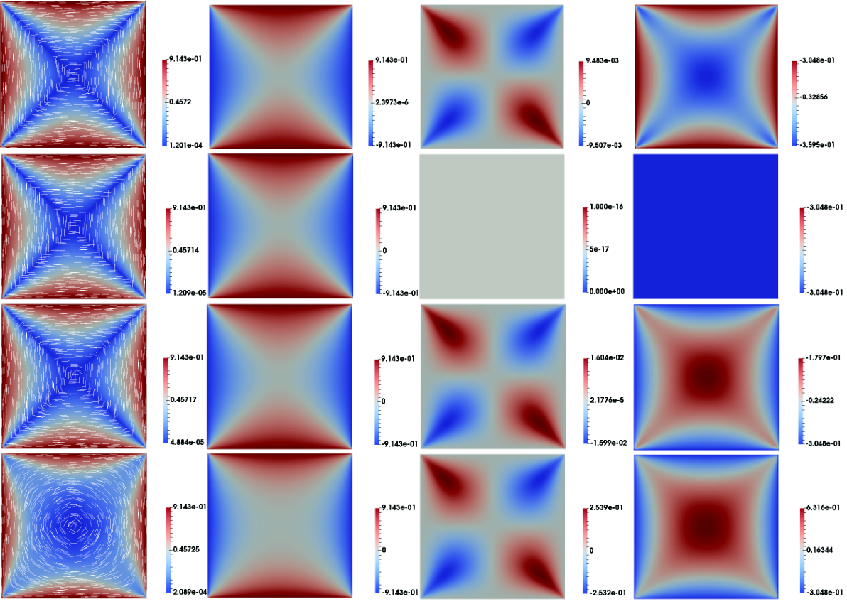
Figure 3.3: The unique stable solution of the Euler-Lagrange equations (3.3)–(3.5), with λ¯2=5\bar{\lambda}^{2}=5, and (from the first to fourth row) L2=−0.5L_{2}=-0.5, 00, 11 and 1010, respectively. In the first column, we plot the scalar order parameter s2=q12+q22s^{2}=q_{1}^{2}+q_{2}^{2} by color from blue to red, and the director profile 𝐧=(cos⁡(a​r​c​t​a​n​(q2/q1)/2),sin⁡(a​r​c​t​a​n​(q2/q1)/2))\mathbf{n}=(\cos(arctan(q_{2}/q_{1})/2),\sin(arctan(q_{2}/q_{1})/2)) in terms of white lines. We plot the corresponding q1,q2q_{1},q_{2} and q3q_{3} profiles, in the second to fourth columns, respectively.

As in wang2019order; canevariharrismajumdarwang, we frequently refer to the following dimensionless parameter in our numerical simulations:

λ¯2:=2​C​λ2L.\displaystyle\bar{\lambda}^{2}:=\frac{2C\lambda^{2}}{L}.

In Figure 3.3, we plot the unique stable solution of (3.3)–(3.5) with λ¯2=5\bar{\lambda}^{2}=5, for L2=−0.5L_{2}=-0.5, 00, 11, 1010. In this figure, and all subsequent figures in this paper, we fix A=−B2/3CA=-B^{2}/3C with B=0.64×10⁴​Nm−2B=0.64\times 10^{4}\,\mathrm{Nm}^{-2} and C=0.35×10⁴​Nm−2C=0.35\times 10^{4}\,\mathrm{Nm}^{-2}. When L2=0L_{2}=0, the solution is the W​O​R​SWORS defined by (3.1). When L2=−0.5L_{2}=-0.5, 11, and 1010, q2q_{2} and q3q_{3} are non-constant as proven above. One can check that q1:Ω→ℝq_{1}:\Omega\to\mathbb{R} vanishes along the square diagonals y=xy=x and y=−xy=-x, and the function q2:Ω→ℝq_{2}:\Omega\to\mathbb{R} vanishes along y=0y=0 and x=0x=0, as proven in Lemma III.5. When L2=−0.5,1,L_{2}=-0.5,1, and 1010, we observe a central +1+1-point defect in the profile of (q1,q2)(q_{1},q_{2}), and we label this as the R​i​n​g+Ring^{+} solution.

Refer to caption
Figure 3.4: A solution branch for the Euler-Lagrange system (3.3)–(3.5) with λ¯2=500\bar{\lambda}^{2}=500, and L2=−0.5L_{2}=-0.5, 00, 11 and 1010 respectively, plotted in the first, second, third and fourth row respectively. This solution branch is a symmetric solution branch, as described in Proposition III.2. When L2=−0.5L_{2}=-0.5, 00 and 11, the plotted solution is unstable. When L2=10L_{2}=10, the plotted solution is stable. The first column contains plots of the order parameter, s2s^{2}, and the director 𝐧\mathbf{n}. In the second to fourth column, we plot the corresponding, q1,q2q_{1},q_{2} and q3q_{3} profiles.

We perform a parameter sweep of λ¯2\bar{\lambda}^{2}, from 55 to 500500, and find one of the symmetric solution branches constructed in Proposition III.2, such that q1:Ω→ℝq_{1}:\Omega\to\mathbb{R} vanishes along the square diagonals y=xy=x and y=−xy=-x and q2:Ω→ℝq_{2}:\Omega\to\mathbb{R} vanishes along y=0y=0 and x=0x=0. This branch is a continuation of the R​i​n​g+Ring^{+} branch. The solutions with λ¯2=500\bar{\lambda}^{2}=500 are plotted in Figure 3.4. When L2=0L_{2}=0, we find the W​O​R​SWORS for all λ>0\lambda>0. When −1<L2<0-1<L_{2}<0, the solution exhibits a +1+1-defect at the square center, continued from the R​i​n​g+Ring^{+} branch and hence, we refer to it as the R​i​n​g+Ring^{+} solution. When L2L_{2} is positive and moderate in value, we recover the R​i​n​g+Ring^{+} solution branch and and the corresponding q3<−s+/6q_{3}<-s_{+}/6 at the square center for negative L2L_{2}, but q3>−s+/6q_{3}>-s_{+}/6 for positive L2L_{2}. When L2L_{2} is large enough, we recover a symmetric solution which is approximately constant, (0,0,s+/3)(0,0,s_{+}/3), away from the square edges, shown in the fourth row of Figure 3.4 for L2=10L_{2}=10. We refer to this solution as the Constant solution in the remainder of this manuscript.

IV Asymptotic Studies

IV.1 The Small λ\lambda and Small Anisotropy L2→0L_{2}\to 0 limit

We work at the special temperature A=−B2/3CA=-B^{2}/3C to facilitate comparison with the results in hansiap2020, where the authors investigate solution landscapes with L2=0.L_{2}=0. Notably, for L2=0L_{2}=0 and A=−B2/3CA=-B^{2}/3C, reduced LdG solutions on 2D polygons have q3≡−s+/6=−B/6Cq_{3}\equiv-s_{+}/6=-B/6C for our choice of TBCs, and it is natural to investigate the effects of the anisotropy parameter, L2L_{2}, on these reduced solutions in 2D frameworks. At A=−B2/3CA=-B^{2}/3C, the governing Euler-Lagrange equations are given by the following system of partial differential equations:

(1+L22)​Δ​q1+L22​(q3,y​y−q3,x​x)\displaystyle\left(1+\frac{L_{2}}{2}\right)\Delta q_{1}+\frac{L_{2}}{2}(q_{3,yy}-q_{3,xx}) =λ2L​q1​(−B23​C+2​B​q3+2​C​(q12+q22+3​q32)),\displaystyle=\frac{\lambda^{2}}{L}q_{1}\left(-\frac{B^{2}}{3C}+2Bq_{3}+2C(q_{1}^{2}+q_{2}^{2}+3q_{3}^{2})\right), (4.1)
(1+L22)​Δ​q2−L2​q3,x​y\displaystyle\left(1+\frac{L_{2}}{2}\right)\Delta q_{2}-L_{2}q_{3,xy} =λ2L​q2​(−B23​C+2​B​q3+2​C​(q12+q22+3​q32)),\displaystyle=\frac{\lambda^{2}}{L}q_{2}\left(-\frac{B^{2}}{3C}+2Bq_{3}+2C(q_{1}^{2}+q_{2}^{2}+3q_{3}^{2})\right), (4.2)
(1+L26)​Δ​q3+L26​(q1,y​y−q1,x​x)−L23​q2,x​y\displaystyle\left(1+\frac{L_{2}}{6}\right)\Delta q_{3}+\frac{L_{2}}{6}(q_{1,yy}-q_{1,xx})-\frac{L_{2}}{3}q_{2,xy} =λ2L​q3​(−B23​C−B​q3+2​C​(q12+q22+3​q32))+λ2​B3​L​(q12+q22),\displaystyle=\frac{\lambda^{2}}{L}q_{3}\left(-\frac{B^{2}}{3C}-Bq_{3}+2C(q_{1}^{2}+q_{2}^{2}+3q_{3}^{2})\right)+\frac{\lambda^{2}B}{3L}(q_{1}^{2}+q_{2}^{2}), (4.3)

satisfying q1=qbq_{1}=q_{b}, q2=0q_{2}=0, and q3=−B/6Cq_{3}=-B/6C on ∂Ω\partial\Omega. We take a regular perturbation expansion of these functions in the L2→0L_{2}\to 0 limit. The leading order approximation is given by the W​O​R​SWORS, (q,0,−B/6C)(q,0,-B/6C), where qq is a solution of the Allen-Cahn equation, as in canevari2017order:

Δq=2​C​λ2Lq(q2−B24​C2),q=qbon∂Ω.\displaystyle\Delta q=\frac{2C\lambda^{2}}{L}q\left(q^{2}-\frac{B^{2}}{4C^{2}}\right),\qquad q=q_{b}\quad\text{on}\quad\partial\Omega. (4.4)

We may assume that q1,q2,q3q_{1},q_{2},q_{3} are expanded in powers of L2L_{2} as follows:

q1​(x,y)\displaystyle q_{1}(x,y) =q⁡(x,y)+L2​f​(x,y)+…\displaystyle=q(x,y)+L_{2}f(x,y)+\dots (4.5)
q2​(x,y)\displaystyle q_{2}(x,y) =L2​g​(x,y)+…\displaystyle=L_{2}g(x,y)+\dots
q3​(x,y)\displaystyle q_{3}(x,y) =−B6​C+L2​h​(x,y)+…\displaystyle=-\frac{B}{6C}+L_{2}h(x,y)+\dots

for some functions f,g,hf,g,h which vanish on the boundary. Up to 𝒪⁡(L2)\mathcal{O}(L_{2}), the governing partial differential equations for f,g,hf,g,h are given by:

Δ​f\displaystyle\Delta f =C​λ2L​(4​q2​f+(2​f−q)​(q2−B24​C2)),\displaystyle=\frac{C\lambda^{2}}{L}\left(4q^{2}f+(2f-q)\left(q^{2}-\frac{B^{2}}{4C^{2}}\right)\right), (4.6)
Δ​g\displaystyle\Delta g =2​C​λ2L​g​(q2−B24​C2),\displaystyle=\frac{2C\lambda^{2}}{L}g\left(q^{2}-\frac{B^{2}}{4C^{2}}\right), (4.7)
Δ​h\displaystyle\Delta h =2​C​λ2Lh(q2+B24​C2)−16(q,yy−q,xx),\displaystyle=\frac{2C\lambda^{2}}{L}h\left(q^{2}+\frac{B^{2}}{4C^{2}}\right)-\frac{1}{6}(q_{,yy}-q_{,xx}), (4.8)

where q=qb,f=g=h=0q=q_{b},f=g=h=0 on ∂Ω\partial\Omega. One can easily verify that the system (4.6)–(4.8), are the Euler-Lagrange equations for the following functional:

F⁡(f,g,h):=\displaystyle F(f,g,h):= ∫Ω{|∇f|2+|∇g|2+|∇h|2+13(q,yh,y−q,xh,x)}dA\displaystyle\int_{\Omega}\left\{|\nabla f|^{2}+|\nabla g|^{2}+|\nabla h|^{2}+\frac{1}{3}(q_{,y}h_{,y}-q_{,x}h_{,x})\right\}\,\mathrm{dA}
+2​C​λ2L∫Ω{(f2+g2)(q2−B24​C2)+h2(q2+B24​C2)−fq(q2−B24​C2−2fq)}dA.\displaystyle+\frac{2C\lambda^{2}}{L}\int_{\Omega}\left\{(f^{2}+g^{2})(q^{2}-\frac{B^{2}}{4C^{2}})+h^{2}(q^{2}+\frac{B^{2}}{4C^{2}})-fq(q^{2}-\frac{B^{2}}{4C^{2}}-2fq)\right\}\,\mathrm{dA}. (4.9)

For λ\lambda small enough, one can show that there exists a unique solution (f,g,h)∈W01,2​(Ω,ℝ3)(f,g,h)\in W^{1,2}_{0}(\Omega;\mathbb{R}^{3}) of the system (4.6)–(4.8), by following the approach in lamy2014 to show that FF is strictly convex in W01,2​(Ω,ℝ3)W^{1,2}_{0}(\Omega;\mathbb{R}^{3}) for sufficiently small λ\lambda. Hence, for λ\lambda small enough, we have g≡0g\equiv 0 on Ω\Omega. Similarly to Proposition III.5, we can check that if (q⁡(x,y),f⁡(x,y),g⁡(x,y),h⁡(x,y))(q(x,y),f(x,y),g(x,y),h(x,y)) is a solution of (4.4),(4.6)–(4.8), then the quadruplets, (−q⁡(y,x),−f⁡(y,x),g⁡(y,x),h⁡(y,x))(-q(y,x),-f(y,x),g(y,x),h(y,x)) and (q⁡(−x,y),f⁡(−x,y),g⁡(−x,y),h⁡(−x,y))(q(-x,y),f(-x,y),g(-x,y),h(-x,y)), are also solutions of (4.4),(4.6)–(4.8). Thus we have f⁡(x,y)=0f(x,y)=0 on diagonals for λ\lambda small enough. Hence, for λ\lambda small enough, the cross structure of the W​O​R​SWORS is lost mainly because of effects of L2L_{2} on the component q3q_{3}, as we discuss below.

From fang2020surface, the solutions of (4.4) with λ=0\lambda=0, are a good approximation to the solutions of (4.4) for sufficiently small λ\lambda. When λ=0\lambda=0, q=q0q=q_{0} where

Δq0=0,(x,y)∈Ω,q0=q1​b,on∂Ω\displaystyle\Delta q_{0}=0,\quad(x,y)\in\Omega,\qquad q_{0}=q_{1b},\quad\text{on}\quad\partial\Omega (4.10)

The analytical solution of (4.10) is given by lewis2015defects:

q0​(x,y)\displaystyle q_{0}(x,y) =s+2​∑k​o​d​d4k​π​(sin⁡(k​π​(x+1)2)​sinh⁡(k​π​(1−y)/2)+sinh⁡(k​π​(1+y)/2)sinh⁡(k​π)CLOSE\displaystyle=\frac{s_{+}}{2}\sum_{k\ odd}\frac{4}{k\pi}\left(\sin\left(\frac{k\pi(x+1)}{2}\right)\frac{\sinh(k\pi(1-y)/2)+\sinh(k\pi(1+y)/2)}{\sinh(k\pi)}\right.
OPEN−sin⁡(k​π​(y+1)2)​sinh⁡(k​π​(1−x)/2)+sinh⁡(k​π​(1+x)/2)sinh⁡(k​π)).\displaystyle\left.-\sin\left(\frac{k\pi(y+1)}{2}\right)\frac{\sinh(k\pi(1-x)/2)+\sinh(k\pi(1+x)/2)}{\sinh(k\pi)}\right). (4.11)

When λ=0\lambda=0, the unique solution of (4.6)–(4.8) is f=f0≡0f=f_{0}\equiv 0, g=g0≡0g=g_{0}\equiv 0 and h=h0h=h_{0} where

Δ​h0=−16​(q0,y​y−q0,x​x),\Delta h_{0}=-\frac{1}{6}(q_{0,yy}-q_{0,xx}), (4.12)

with h0=0h_{0}=0 on ∂Ω\partial\Omega. In Figure 4.5, we plot the difference between the solution, (q1,q2,q3)(q_{1},q_{2},q_{3}) of (4.3) and the triplet, (q0+L2​f0,L2​g0,−s+6+L2​h0)=(q0,0,−s+6+L2​h0)(q_{0}+L_{2}f_{0},L_{2}g_{0},-\frac{s_{+}}{6}+L_{2}h_{0})=(q_{0},0,-\frac{s_{+}}{6}+L_{2}h_{0}), which is the solution of (4.6)-(4.8) for λ=0\lambda=0.

Proposition IV.1.

The analytical solution of (4.12) is given by

h0​(x,y)=∑m,n​o​d​d16​s+​m​n3​π2​(m2+n2)2​sin⁡(m​π​(x+1)2)​sin⁡(n​π​(y+1)2),h_{0}(x,y)=\sum_{m,n\ odd}\frac{16s_{+}mn}{3\pi^{2}(m^{2}+n^{2})^{2}}\sin\left(\frac{m\pi(x+1)}{2}\right)\sin\left(\frac{n\pi(y+1)}{2}\right), (4.13)

where h0​(0,0)h_{0}(0,0) is positive.

Proof.

Firstly, we calculate the analytical solution of (4.12). Substituting (IV.1) into (4.12), we have

Δ​h0\displaystyle\Delta h_{0} =−∑k​o​d​ds+​k​π6​sinh⁡(k​π){sin(k​π​(x+1)2)(sinh(k​π​(1−y)2)+sinh(k​π​(1+y)2))\displaystyle=-\sum_{k\ odd}\frac{s_{+}k\pi}{6\sinh(k\pi)}\left\{\sin\left(\frac{k\pi(x+1)}{2}\right)\left(\sinh\left(\frac{k\pi(1-y)}{2}\right)+\sinh\left(\frac{k\pi(1+y)}{2}\right)\right)\right.
+sin(k​π​(y+1)2)(sinh(k​π​(1−x)2)+sinh(k​π​(1+x)2))},\displaystyle\left.+\sin\left(\frac{k\pi(y+1)}{2}\right)\left(\sinh\left(\frac{k\pi(1-x)}{2}\right)+\sinh\left(\frac{k\pi(1+x)}{2}\right)\right)\right\}, (4.14)

which is a homogeneous Poisson equation. We consider the transformations x^=x+1\hat{x}=x+1 and y^=y+1\hat{y}=y+1, such that h0​(x^,y^):[0,2]2→ℝh_{0}(\hat{x},\hat{y}):[0,2]^{2}\to\mathbb{R}. We apply the method of eigenfunction expansions

h0​(x^,y^)=∑n=1∞∑m=1∞Em​n​sin⁡(m​π​x^2)​sin⁡(n​π​y^2),\displaystyle h_{0}(\hat{x},\hat{y})=\sum_{n=1}^{\infty}\sum_{m=1}^{\infty}E_{mn}\sin\left(\frac{m\pi\hat{x}}{2}\right)\sin\left(\frac{n\pi\hat{y}}{2}\right), (4.15)

where Em​nE_{mn} are double Fourier sine series coefficients. Following standard Fourier series-type calculations, we obtain:

h0​(x^,y^)=∑m,n​o​d​d16​s+​m​n3​π2​(m2+n2)2​sin⁡(m​π​x^2)​sin⁡(n​π​y^2),\displaystyle h_{0}(\hat{x},\hat{y})=\sum_{m,n\ odd}\frac{16s_{+}mn}{3\pi^{2}(m^{2}+n^{2})^{2}}\sin\left(\frac{m\pi\hat{x}}{2}\right)\sin\left(\frac{n\pi\hat{y}}{2}\right), (4.16)

which yields the form (4.13). Substituting (x,y)=(0,0)(x,y)=(0,0) i.e., (x^,y^)=(1,1)(\hat{x},\hat{y})=(1,1) into (4.13), we obtain

h0​(1,1)\displaystyle h_{0}(1,1) =16​s+3​π2​∑m,n​o​d​dm​n(m2+n2)2​sin⁡(m​π2)​sin⁡(n​π2)\displaystyle=\frac{16s_{+}}{3\pi^{2}}\sum_{m,n\ odd}\frac{mn}{(m^{2}+n^{2})^{2}}\sin\left(\frac{m\pi}{2}\right)\sin\left(\frac{n\pi}{2}\right)
=16​s+3​π2​∑m,n​o​d​dm​n(m2+n2)2​(−1)m+n−22\displaystyle=\frac{16s_{+}}{3\pi^{2}}\sum_{m,n\ odd}\frac{mn}{(m^{2}+n^{2})^{2}}(-1)^{\frac{m+n-2}{2}}
=16​s+3​π2​∑m​o​d​d14​m2+32​s+3​π2​∑m>n​o​d​dm​n(m2+n2)2​(−1)m+n−22\displaystyle=\frac{16s_{+}}{3\pi^{2}}\sum_{m\ odd}\frac{1}{4m^{2}}+\frac{32s_{+}}{3\pi^{2}}\sum_{m>n\ odd}\frac{mn}{(m^{2}+n^{2})^{2}}(-1)^{\frac{m+n-2}{2}}
=s+6+32​s+3​π2​∑m>n​o​d​dm​n(m2+n2)2​(−1)m+n−22\displaystyle=\frac{s_{+}}{6}+\frac{32s_{+}}{3\pi^{2}}\sum_{m>n\ odd}\frac{mn}{(m^{2}+n^{2})^{2}}(-1)^{\frac{m+n-2}{2}} (4.17)

The summed term in (4.17) is

∑m>n​o​d​dm​n(m2+n2)2​(−1)m+n−22\displaystyle\sum_{m>n\ odd}\frac{mn}{(m^{2}+n^{2})^{2}}(-1)^{\frac{m+n-2}{2}} =∑n​o​d​d,m=n+4​s−2m​n(m2+n2)2​(−1)m+n−22\displaystyle=\sum_{n\ odd,m=n+4s-2}\frac{mn}{(m^{2}+n^{2})^{2}}(-1)^{\frac{m+n-2}{2}}
+∑n​o​d​d,m=n+4​sm​n(m2+n2)2(−1)m+n−22\displaystyle+\sum_{n\ odd,m=n+4s}\frac{mn}{(m^{2}+n^{2})^{2}}(-1)^{\frac{m+n-2}{2}}
≥∑n​o​d​d,m=n+4​s−2m​n(m2+n2)2​(−1)m+n−22\displaystyle\geq\sum_{n\ odd,m=n+4s-2}\frac{mn}{(m^{2}+n^{2})^{2}}(-1)^{\frac{m+n-2}{2}} (4.18)

Setting k=m+nk=m+n, l=m−nl=m-n, we have m​n/(m2+n2)2=(k2−l2)/(k2+l2)2mn/(m^{2}+n^{2})^{2}=(k^{2}-l^{2})/(k^{2}+l^{2})^{2}. Since nn is odd, we have k=m+n=2​n+4​s−2=2​(2​p+1)+4​s−2=4​(p+s)=4​rk=m+n=2n+4s-2=2(2p+1)+4s-2=4(p+s)=4r, (p≥0,s,r≥1)(p\geq 0,s,r\geq 1), and l=m−n=4​s−2l=m-n=4s-2. Substituting k=m+nk=m+n, l=m−nl=m-n into (4.18), we obtain

∑n​o​d​d,m=n+4​s−2m​n(m2+n2)2​(−1)m+n−22\displaystyle\sum_{n\ odd,m=n+4s-2}\frac{mn}{(m^{2}+n^{2})^{2}}(-1)^{\frac{m+n-2}{2}} =∑k>l,k=4​r,l=4​s−2k2−l2(k2+l2)2​(−1)k−22\displaystyle=\sum_{k>l,k=4r,l=4s-2}\frac{k^{2}-l^{2}}{(k^{2}+l^{2})^{2}}(-1)^{\frac{k-2}{2}}
=−∑k>l,k=4​r,l=4​s−2k2−l2(k2+l2)2\displaystyle=-\sum_{k>l,k=4r,l=4s-2}\frac{k^{2}-l^{2}}{(k^{2}+l^{2})^{2}}
≥−∑k=4​r1k2=−∑r=1∞116​r2=−π296\displaystyle\geq-\sum_{k=4r}\frac{1}{k^{2}}=-\sum_{r=1}^{\infty}\frac{1}{16r^{2}}=-\frac{\pi^{2}}{96} (4.19)

Hence, from (4.17) we have h0​(0,0)≥s+6−s+9>0h_{0}(0,0)\geq\frac{s_{+}}{6}-\frac{s_{+}}{9}>0. ∎

Refer to caption
Figure 4.5: First row: plots of (q1,q2,q3)(q_{1},q_{2},q_{3}), the solution of (3.3)–(3.5) with λ¯2=0.01\bar{\lambda}^{2}=0.01, L2=0.1L_{2}=0.1. Second row: plots of asymptotic solution (q0+L2​f0,L2​g0,−s+6+L2​h0)=(q0,0,−s+6+L2​h0)(q_{0}+L_{2}f_{0},L_{2}g_{0},-\frac{s_{+}}{6}+L_{2}h_{0})=(q_{0},0,-\frac{s_{+}}{6}+L_{2}h_{0}), where q0q_{0} and h0h_{0} are the solutions of (4.10) and (4.12), respectively. Third row: plots of the difference between solution in first and second row, (q1,q2,q3)−(q0+L2​f0,L2​g0,−s+6+L2​h0)(q_{1},q_{2},q_{3})-(q_{0}+L_{2}f_{0},L_{2}g_{0},-\frac{s_{+}}{6}+L_{2}h_{0}).

IV.2 The L2→+∞L_{2}\to+\infty limit

Consider the regular perturbation expansion in powers of 1/L21/L_{2} of the solutions, q1,q2,q3q_{1},q_{2},q_{3}, of the Euler-Lagrange system (3.3)–(3.5) subject to the boundary conditions (2.14) and (2.15). Then the governing Euler-Lagrange equations (3.3)–(3.5) to leading order that is, 𝒪⁡(L2)\mathcal{O}(L_{2}), are given by the following system of PDEs:

12​Δ​ρ+12​(τy​y−τx​x)\displaystyle\frac{1}{2}\Delta\rho+\frac{1}{2}(\tau_{yy}-\tau_{xx}) =0,\displaystyle=0, (4.20)
12​Δ​σ−τx​y\displaystyle\frac{1}{2}\Delta\sigma-\tau_{xy} =0,\displaystyle=0, (4.21)
16​Δ​τ+16​(ρy​y−ρx​x)−13​σx​y\displaystyle\frac{1}{6}\Delta\tau+\frac{1}{6}(\rho_{yy}-\rho_{xx})-\frac{1}{3}\sigma_{xy} =0,\displaystyle=0, (4.22)

where the ρ,σ,τ\rho,\sigma,\tau are the leading order approximations of q1,q2,q3q_{1},q_{2},q_{3}, respectively in the L2→∞L_{2}\to\infty limit.

Proposition IV.2.

The leading order system of Euler-Lagrange equations in the L2→∞L_{2}\to\infty limit, (4.20)–(4.22), is not an elliptic PDE system.

Proof.

The system of equations (4.20)–(4.22) can be written as

A​𝐪0,x​x+2​B​𝐪0,x​y+C​𝐪0,y​y=𝟎,\displaystyle A\mathbf{q}_{0,xx}+2B\mathbf{q}_{0,xy}+C\mathbf{q}_{0,yy}=\mathbf{0},

where 𝐪0=(ρ,σ,τ)\mathbf{q}_{0}=(\rho,\sigma,\tau) and

A=(120−120120−16016),B=(00000−120−160),C=(12012012016016).\displaystyle A=\begin{pmatrix}\frac{1}{2}&0&-\frac{1}{2}\\ 0&\frac{1}{2}&0\\ -\frac{1}{6}&0&\frac{1}{6}\end{pmatrix},\quad B=\begin{pmatrix}0&0&0\\ 0&0&-\frac{1}{2}\\ 0&-\frac{1}{6}&0\end{pmatrix},\quad C=\begin{pmatrix}\frac{1}{2}&0&\frac{1}{2}\\ 0&\frac{1}{2}&0\\ \frac{1}{6}&0&\frac{1}{6}\end{pmatrix}.

The system is said to be elliptic, in the sense of I.G. Petrovsky Gu, if the determinant

|A​α2+2​B​α​β+C​β2|≠0,\displaystyle|A\alpha^{2}+2B\alpha\beta+C\beta^{2}|\neq 0,

for any real numbers α,β≠0\alpha,\beta\neq 0. We can check that for this system, we have

|A​α2+2​B​α​β+C​β2|≡0.\displaystyle|A\alpha^{2}+2B\alpha\beta+C\beta^{2}|\equiv 0.

for any real numbers α,β\alpha,\beta. Hence, the limiting problem (4.20)–(4.22) is not an elliptic problem. ∎

Proposition IV.3.

There is no classical solution of the limiting problem (4.20)–(4.22), with the boundary conditions (2.14) in the ϵ→0\epsilon\to 0 limit and (2.15), where ϵ\epsilon is the short edge length of the truncated unit square, Ω\Omega.

Proof.

As L2→∞L_{2}\to\infty, the minimizers (q1,q2,q3)(q_{1},q_{2},q_{3}) of the energy JJ in (3.6), with fe​lf_{el} as in (3.10), are constrained to satisfy

fd​i​v​(q1,q2,q3)=(q1,x+q2,y−q3,x)2+(q2,x−q1,y−q3,y)2=0,a.e.(x,y)∈Ω,\displaystyle f_{div}(q_{1},q_{2},q_{3})=(q_{1,x}+q_{2,y}-q_{3,x})^{2}+(q_{2,x}-q_{1,y}-q_{3,y})^{2}=0,\quad\text{a.e.}\quad(x,y)\in\Omega,

subject to the Dirichlet TBCs (2.14) and (2.15). Up to 𝒪⁡(L2)\mathcal{O}(L_{2}), this corresponds to the following PDEs for the leading order approximations ρ,σ,τ\rho,\sigma,\tau:

(ρ−τ)x+σy=0,\displaystyle(\rho-\tau)_{x}+\sigma_{y}=0, (4.23)
σx−(ρ+τ)y=0,\displaystyle\sigma_{x}-(\rho+\tau)_{y}=0, (4.24)

almost everywhere, subject to the same TBCs, ρ=qb\rho=q_{b}, σ=0\sigma=0, τ=−s+/6\tau=-s_{+}/6 on ∂Ω\partial\Omega. As ϵ→0\epsilon\to 0, the boundary conditions for ρ,σ,τ\rho,\sigma,\tau are piecewise constant, and hence the tangential derivatives of ρ,σ\rho,\sigma and τ\tau vanish on the long square edges. On y=±1y=\pm 1, the tangential derivative (ρ−τ)x=0(\rho-\tau)_{x}=0, hence we obtain σy=0\sigma_{y}=0 in (4.23). Similarly, we have σx=0\sigma_{x}=0 on x=±1x=\pm 1. This implies that ∂νσ=0\partial_{\nu}\sigma=0 on ∂Ω\partial\Omega, where ∂ν\partial_{\nu} is the outward pointing normal derivative, and we view the equation (4.21) to be of the form

Δ​σ=u⁡(x,y),σ|∂Ω=0.\displaystyle\Delta\sigma=u(x,y),\qquad\left.\sigma\right|_{\partial\Omega}=0.

By the Hopf Lemma, when ∂ν=0\partial_{\nu}=0, we have σ≡0\sigma\equiv 0. Following the same arguments as in Proposition III.3, this requires that τ≡−s+/6\tau\equiv-s_{+}/6. Substituting τ≡−s+/6\tau\equiv-s_{+}/6 into equations (4.23) and (4.24), we obtain ρx=ρy=0\rho_{x}=\rho_{y}=0, contradicting the boundary condition (2.14). Hence, there are no classical solutions of the system (4.20)–(4.22). ∎

Although there is no classical solution of (4.20)–(4.22) subject to the imposed boundary conditions, we can use finite difference methods to calculate a numerical solution, see Figure 4.6. We label this solution (ρ,σ,τ)≡(0,0,s+/3)(\rho,\sigma,\tau)\equiv(0,0,s_{+}/3) on Ω\Omega as the Constant solution, where ρ\rho and τ\tau are discontinuous on ∂Ω\partial\Omega.

Refer to caption
Figure 4.6: Solutions, ρ,σ,τ\rho,\sigma,\tau, of the leading order Euler-Lagrange system (4.20)–(4.22) in the L2→∞L_{2}\to\infty limit. Plots of (from left to right) ρ,σ,τ\rho,\sigma,\tau, and (x,y,τ)(x,y,\tau).

We now give a heuristic argument to explain the emergence of the Constant solution in the interior of Ω\Omega, as L2→∞L_{2}\to\infty. Assuming ρ=a\rho=a, σ=b\sigma=b, and τ=c\tau=c, where a,b,c∈ℝa,b,c\in\mathbb{R} are constants, we have fd​i​v=0f_{div}=0 in Ω\Omega up to 𝒪⁡(L2)\mathcal{O}(L_{2}). On the boundary, using finite difference methods, the first derivatives e.g., ρx\rho_{x}, are calculated from the difference between the interior value and the value on the boundary i.e., ρx|x=−1=(ρ|i​n​t​e​r​i​o​r−ρ|b​o​u​n​d​a​r​y)/h=(a−(−s+/2))/h\rho_{x}|_{x=-1}=(\rho|_{interior}-\rho|_{boundary})/h=(a-(-s_{+}/2))/h, where hh is the size of square mesh. We compute the choices of a,ba,b, and cc, that ensure fd​i​v=0f_{div}=0 on the boundary, below:

(a+s+2−c−s+6)2+b2\displaystyle(a+\frac{s_{+}}{2}-c-\frac{s_{+}}{6})^{2}+b^{2} =0on​x=−1,\displaystyle=0\quad\text{on}\,\,x=-1,
(−a−s+2+c+s+6)2+(−b)2\displaystyle(-a-\frac{s_{+}}{2}+c+\frac{s_{+}}{6})^{2}+(-b)^{2} =0on​x=1,\displaystyle=0\quad\text{on}\,\,x=1,
b2+(−a+s+2−c−s+6)2\displaystyle b^{2}+(-a+\frac{s_{+}}{2}-c-\frac{s_{+}}{6})^{2} =0on​y=−1,\displaystyle=0\quad\text{on}\,\,y=-1,
(−b)2+(a−s+2+c+s+6)2\displaystyle(-b)^{2}+(a-\frac{s_{+}}{2}+c+\frac{s_{+}}{6})^{2} =0on​y=1,\displaystyle=0\quad\text{on}\,\,y=1,

and hence a=b=0a=b=0, c=s+/3c=s_{+}/3. Therefore, ρ=σ=0\rho=\sigma=0, τ=s+/3\tau=s_{+}/3 is the unique stable solution of (4.20)–(4.21), except for zero measure sets and we label (q1,q2,q3)=(0,0,s+/3)(q_{1},q_{2},q_{3})=(0,0,s_{+}/3) as the physically relevant Constant solution in the L2→∞L_{2}\to\infty limit. This is consistent with the numerical results in Figure 3.3.

IV.3 The λ→∞\lambda\to\infty limit

The set of minimizers of the thermotropic bulk energy density, fbf_{b}, in the (q1,q2,q3)(q_{1},q_{2},q_{3})-plane can be written as 𝕊=𝕊1∪𝕊2\mathbb{S}=\mathbb{S}_{1}\cup\mathbb{S}_{2}, where

𝕊1={(q1,q2,q3):q12+q22=s+24,q3=−s+6},𝕊2=(0,0,s+3).\displaystyle\mathbb{S}_{1}=\left\{(q_{1},q_{2},q_{3}):q_{1}^{2}+q_{2}^{2}=\frac{s_{+}^{2}}{4},\,\,q_{3}=-\frac{s_{+}}{6}\right\},\qquad\mathbb{S}_{2}=\left(0,0,\frac{s_{+}}{3}\right). (4.25)

The λ→∞\lambda\to\infty limit is equivalent to the vanishing elastic constant limit, and the bulk energy density, fbf_{b}, converges uniformly to its minimum value in this limit majumdar2010landau.

Proposition IV.4.

Let Ω∈ℝ2\Omega\in\mathbb{R}^{2} be a simply connected bounded open set with smooth boundary. Let (q1λ,q2λ,q3λ)(q_{1}^{\lambda},q_{2}^{\lambda},q_{3}^{\lambda}) be a global minimizer of J⁡(q1,q2,q3)J(q_{1},q_{2},q_{3}) in the admissible class 𝒜0\mathcal{A}_{0} in (3.9), when L2>−1L_{2}>-1. Then there exists a sequence λk→∞\lambda_{k}\to\infty such that (q1λk,q2λk,q3λk)→(q1∞,q2∞,q3∞)(q_{1}^{\lambda_{k}},q_{2}^{\lambda_{k}},q_{3}^{\lambda_{k}})\to(q_{1}^{\infty},q_{2}^{\infty},q_{3}^{\infty}) strongly in W1,2​(Ω,ℝ3)W^{1,2}(\Omega;\mathbb{R}^{3}) where (q1∞,q2∞,q3∞)∈𝕊(q_{1}^{\infty},q_{2}^{\infty},q_{3}^{\infty})\in\mathbb{S}. If (q1∞,q2∞,q3∞)∈𝕊1(q_{1}^{\infty},q_{2}^{\infty},q_{3}^{\infty})\in\mathbb{S}_{1}, i.e.,

q1∞=s+2​cos⁡(2​θ∞),q2∞=s+2​sin⁡(2​θ∞),q3∞=−s+6,\displaystyle q_{1}^{\infty}=\frac{s_{+}}{2}\cos(2\theta^{\infty}),\quad q_{2}^{\infty}=\frac{s_{+}}{2}\sin(2\theta^{\infty}),\quad q_{3}^{\infty}=-\frac{s_{+}}{6}, (4.26)

then θ∞\theta^{\infty} is a minimizer of

∫Ω|∇θ|2​dA,\int_{\Omega}|\nabla\theta|^{2}\textrm{dA}, (4.27)

in the admissible class

𝒜θ={θ∈W1,2​(Ω);θ=θb​o​n​∂Ω},\mathcal{A}_{\theta}=\{\theta\in W^{1,2}(\Omega);\theta=\theta_{b}\ on\ \partial\Omega\}, (4.28)

The boundary condition, θb\theta_{b}, is compatible with (q1,q2)(q_{1},q_{2}) on ∂Ω\partial\Omega by the relation (q1​b,q2​b)=s+2​(cos⁡(2​θb),sin⁡(2​θb))(q_{1b},q_{2b})=\frac{s_{+}}{2}(\cos(2\theta_{b}),\sin(2\theta_{b})). Otherwise, (q1∞,q2∞,q3∞)​(x,y)∈𝕊2(q_{1}^{\infty},q_{2}^{\infty},q_{3}^{\infty})(x,y)\in\mathbb{S}_{2}, i.e.,

(q1∞,q2∞,q3∞)=(0,0,s+3).\displaystyle(q_{1}^{\infty},q_{2}^{\infty},q_{3}^{\infty})=\left(0,0,\frac{s_{+}}{3}\right). (4.29)
Proof.

Our proof is analogous to Lemma 3 of majumdar2010landau. Firstly, we note that (q1∞,q2∞,q3∞)(q_{1}^{\infty},q_{2}^{\infty},q_{3}^{\infty}) belongs to admissible space 𝒜0\mathcal{A}_{0}. As in Proposition III.4, we can show that the W1,2W^{1,2}-norms of the (q1λ,q2λ,q3λ)(q_{1}^{\lambda},q_{2}^{\lambda},q_{3}^{\lambda})’s are uniformly bounded. Hence there exists a weakly-convergent subsequence (q1λk,q2λk,q3λk)(q_{1}^{\lambda_{k}},q_{2}^{\lambda_{k}},q_{3}^{\lambda_{k}}) such that (q1λk,q2λk,q3λk)⇀(q11,q21,q31)(q_{1}^{\lambda_{k}},q_{2}^{\lambda_{k}},q_{3}^{\lambda_{k}})\rightharpoonup(q_{1}^{1},q_{2}^{1},q_{3}^{1}) in W1,2W^{1,2}, for some (q11,q21,q31)∈𝒜0(q_{1}^{1},q_{2}^{1},q_{3}^{1})\in\mathcal{A}_{0} as λk→∞\lambda_{k}\to\infty. Using the lower semicontinuity of the W1,2W^{1,2} norm with respect to the weak convergence, we have that

∫Ω|∇(q11,q21,q31)|2​dA≤∫Ω|∇(q1∞,q2∞,q3∞)|2​dA\int_{\Omega}|\nabla(q_{1}^{1},q_{2}^{1},q_{3}^{1})|^{2}\,\textrm{dA}\leq\int_{\Omega}|\nabla(q_{1}^{\infty},q_{2}^{\infty},q_{3}^{\infty})|^{2}\,\textrm{dA} (4.30)

The relation in (3.35) shows that ∫Ωf¯b​(q1λk,q2λk,q3λk)​dA≤1λk2​∫Ωfe​l​(q1∞,q2∞,q3∞)​dA\int_{\Omega}\bar{f}_{b}(q_{1}^{\lambda_{k}},q_{2}^{\lambda_{k}},q_{3}^{\lambda_{k}})\,\textrm{dA}\leq\frac{1}{\lambda_{k}^{2}}\int_{\Omega}f_{el}(q_{1}^{\infty},q_{2}^{\infty},q_{3}^{\infty})\,\textrm{dA}, where f¯b=1L​(fb−min⁡fb)\bar{f}_{b}=\frac{1}{L}(f_{b}-\min f_{b}), and hence

∫Ωf¯b​(q1λk,q2λk,q3λk)​dA→0a​sλk→∞.\displaystyle\int_{\Omega}\bar{f}_{b}(q_{1}^{\lambda_{k}},q_{2}^{\lambda_{k}},q_{3}^{\lambda_{k}})\,\textrm{dA}\to 0\quad as\quad\lambda_{k}\to\infty. (4.31)

Since f¯b​(q1,q2,q3)≥0\bar{f}_{b}(q_{1},q_{2},q_{3})\geq 0, ∀(q1,q2,q3)∈ℝ3\forall(q_{1},q_{2},q_{3})\in\mathbb{R}^{3} we have that, on a subsequence λkj\lambda_{k_{j}},

f¯b​(q1λkj​(𝐱),q2λkj​(𝐱),q3λkj​(𝐱))→0,\displaystyle\bar{f}_{b}(q_{1}^{\lambda_{k_{j}}}(\mathbf{x}),q_{2}^{\lambda_{k_{j}}}(\mathbf{x}),q_{3}^{\lambda_{k_{j}}}(\mathbf{x}))\to 0, (4.32)

for almost all 𝐱∈Ω\mathbf{x}\in\Omega. We know that f¯b​(q1,q2,q3)=0\bar{f}_{b}(q_{1},q_{2},q_{3})=0 if, and only if, (q1,q2,q3)∈𝕊(q_{1},q_{2},q_{3})\in\mathbb{S}. On the other hand, the sequence (q1λk,q2λk,q3λk)(q_{1}^{\lambda_{k}},q_{2}^{\lambda_{k}},q_{3}^{\lambda_{k}}) converges weakly in W1,2W^{1,2} and, on a subsequence, strongly in L2L^{2} to (q11,q21,q31)(q_{1}^{1},q_{2}^{1},q_{3}^{1}). Therefore, the weak limit (q11​(x),q21​(x),q31​(x))(q_{1}^{1}(x),q_{2}^{1}(x),q_{3}^{1}(x)) is in the set 𝕊\mathbb{S} a.e. 𝐱∈Ω\mathbf{x}\in\Omega. If (q11​(x),q21​(x),q31​(x))(q_{1}^{1}(x),q_{2}^{1}(x),q_{3}^{1}(x)) is in the set 𝕊1\mathbb{S}_{1}, then |∇(q11,q21,q31)|2=s+2​|∇θ1|2|\nabla(q_{1}^{1},q_{2}^{1},q_{3}^{1})|^{2}=s_{+}^{2}|\nabla\theta^{1}|^{2}, where q11=s+2​cos⁡(2​θ1)q_{1}^{1}=\frac{s_{+}}{2}\cos(2\theta^{1}) and q21=s+2​sin⁡(2​θ1)q_{2}^{1}=\frac{s_{+}}{2}\sin(2\theta^{1}). In this case, we take (q1∞,q2∞,q3∞)∈𝕊1(q_{1}^{\infty},q_{2}^{\infty},q_{3}^{\infty})\in\mathbb{S}_{1} as defined above, so that |∇(q1∞,q2∞,q3∞)|2=s+2​|∇θ∞|2|\nabla(q_{1}^{\infty},q_{2}^{\infty},q_{3}^{\infty})|^{2}=s_{+}^{2}|\nabla\theta^{\infty}|^{2}, where q1∞=s+2​cos⁡(2​θ∞)q_{1}^{\infty}=\frac{s_{+}}{2}\cos(2\theta^{\infty}) and q2∞=s+2​sin⁡(2​θ∞)q_{2}^{\infty}=\frac{s_{+}}{2}\sin(2\theta^{\infty}). If (q11​(x),q21​(x),q31​(x))(q_{1}^{1}(x),q_{2}^{1}(x),q_{3}^{1}(x)) is in the set 𝕊2\mathbb{S}_{2}, then we take (q1∞,q2∞,q3∞)=(q11,q21,q31)=(0,0,s+/3)(q_{1}^{\infty},q_{2}^{\infty},q_{3}^{\infty})=(q_{1}^{1},q_{2}^{1},q_{3}^{1})=(0,0,s_{+}/3). Combining (4.30) with the definition of (q1∞,q2∞,q2∞)(q_{1}^{\infty},q_{2}^{\infty},q_{2}^{\infty}), we obtain that ∫Ω|∇θ1|2​dA=∫Ω|∇θ∞|2​dA\int_{\Omega}|\nabla\theta^{1}|^{2}\,\textrm{dA}=\int_{\Omega}|\nabla\theta^{\infty}|^{2}\,\textrm{dA} and ∫Ω|∇(q11,q21,q31)|2​dA=∫Ω|∇(q1∞,q2∞,q3∞)|2​dA\int_{\Omega}|\nabla(q_{1}^{1},q_{2}^{1},q_{3}^{1})|^{2}\,\textrm{dA}=\int_{\Omega}|\nabla(q_{1}^{\infty},q_{2}^{\infty},q_{3}^{\infty})|^{2}\,\textrm{dA}. Therefore,

∫Ω|∇(q1∞,q2∞,q3∞)|2​dA\displaystyle\int_{\Omega}|\nabla(q_{1}^{\infty},q_{2}^{\infty},q_{3}^{\infty})|^{2}\,\textrm{dA} ≤lim infλkj→∞∫Ω|∇(q1λkj,q2λkj,q3λkj)|2​dA\displaystyle\leq\liminf_{\lambda_{k_{j}}\to\infty}\int_{\Omega}|\nabla(q_{1}^{\lambda_{k_{j}}},q_{2}^{\lambda_{k_{j}}},q_{3}^{\lambda_{k_{j}}})|^{2}\,\textrm{dA} (4.33)
≤lim supλkj→∞∫Ω|∇(q1λkj,q2λkj,q3λkj)|2​dA\displaystyle\leq\limsup_{\lambda_{k_{j}}\to\infty}\int_{\Omega}|\nabla(q_{1}^{\lambda_{k_{j}}},q_{2}^{\lambda_{k_{j}}},q_{3}^{\lambda_{k_{j}}})|^{2}\,\textrm{dA} (4.34)
≤∫Ω|∇(q1∞,q2∞,q3∞)|2​dA,\displaystyle\leq\int_{\Omega}|\nabla(q_{1}^{\infty},q_{2}^{\infty},q_{3}^{\infty})|^{2}\,\textrm{dA}, (4.35)

which demonstrates that limλkj→∞‖∇(q1λkj,q2λkj,q3λkj)‖L2=‖∇(q1∞,q2∞,q3∞)‖L2\lim\limits_{\lambda_{k_{j}}\to\infty}||\nabla(q_{1}^{\lambda_{k_{j}}},q_{2}^{\lambda_{k_{j}}},q_{3}^{\lambda_{k_{j}}})||_{L^{2}}=||\nabla(q_{1}^{\infty},q_{2}^{\infty},q_{3}^{\infty})||_{L^{2}}. This together with the weak convergence (q1λkj,q2λkj,q3λkj)→(q1∞,q2∞,q3∞)(q_{1}^{\lambda_{k_{j}}},q_{2}^{\lambda_{k_{j}}},q_{3}^{\lambda_{k_{j}}})\to(q_{1}^{\infty},q_{2}^{\infty},q_{3}^{\infty}) suffices to show the strong convergence (q1λkj,q2λkj,q3λkj)→(q1∞,q2∞,q3∞)(q_{1}^{\lambda_{k_{j}}},q_{2}^{\lambda_{k_{j}}},q_{3}^{\lambda_{k_{j}}})\to(q_{1}^{\infty},q_{2}^{\infty},q_{3}^{\infty}) in W1,2W^{1,2}. Since fb​(q1∞,q2∞,q3∞)f_{b}(q_{1}^{\infty},q_{2}^{\infty},q_{3}^{\infty}) is constant for (q1∞,q2∞,q3∞)∈𝕊1(q_{1}^{\infty},q_{2}^{\infty},q_{3}^{\infty})\in\mathbb{S}_{1}, we can recast our minimization problem to minimizing the elastic energy alone i.e., minimization of the limiting functional:

J∞​[q1,q2,q3]=∫Ωfe​l​(q1,q2,q3)​dA.J_{\infty}[q_{1},q_{2},q_{3}]=\int_{\Omega}f_{el}\left(q_{1},q_{2},q_{3}\right)\,\mathrm{dA}. (4.36)

Substituting

q1=s+2​cos⁡(2​θ),q2=s+2​sin⁡(2​θ),q3=−s+6,\displaystyle q_{1}=\frac{s_{+}}{2}\cos(2\theta),\quad q_{2}=\frac{s_{+}}{2}\sin(2\theta),\quad q_{3}=-\frac{s_{+}}{6}, (4.37)

into (4.36), we have that

J∞=s+2​(1+L22)​∫Ω|∇θ|2​dA.\displaystyle J_{\infty}=s_{+}^{2}\left(1+\frac{L_{2}}{2}\right)\int_{\Omega}|\nabla\theta|^{2}\,\mathrm{dA}. (4.38)

The corresponding Euler-Lagrange equation for (4.27) is simply the Laplace equation

Δ​θ=0,\Delta\theta=0, (4.39)

subject to θ=θb\theta=\theta_{b} on ∂Ω\partial\Omega, where (q1,q2,q3)=(s+2​cos⁡(2​θb),s+2​sin⁡(2​θb),−s+6)(q_{1},q_{2},q_{3})=(\frac{s_{+}}{2}\cos(2\theta_{b}),\frac{s_{+}}{2}\sin(2\theta_{b}),-\frac{s_{+}}{6}) on ∂Ω\partial\Omega. ∎

For large λ\lambda i.e., large square domains, there are two classes of stable equilibria which are almost in the set 𝕊1\mathbb{S}_{1}. The diagonal states, DD, are such that the nematic director (in the plane) is aligned along one of the square diagonals. The rotated states, labelled as RR states, are such that the director rotates by π\pi radians between a pair of opposite square edges. There are 22 rotationally equivalent DD states, and 44 rotationally equivalent RR states. The corresponding boundary conditions in terms of θ\theta are given by θb=θbD\theta_{b}=\theta_{b}^{D} or θbR\theta_{b}^{R} respectively, where

{θbD=π2,onx=±1,θbD=0,ony=±1,{θbR=π2,onx=−1,θbR=−π2,onx=1,θbR=0,ony=±1.\displaystyle\begin{cases}\theta_{b}^{D}&=\frac{\pi}{2},\ \text{on}\ x=\pm 1,\\ \theta_{b}^{D}&=0,\ \text{on}\ y=\pm 1,\end{cases}\qquad\begin{cases}\theta_{b}^{R}&=\frac{\pi}{2},\ \text{on}\ x=-1,\\ \theta_{b}^{R}&=-\frac{\pi}{2},\ \text{on}\ x=1,\\ \theta_{b}^{R}&=0,\ \text{on}\ y=\pm 1.\end{cases} (4.40)
Refer to caption
Figure 4.7: The DD and RR solutions of the Euler-Lagrange equation (3.3)–(3.5) with L2=3.5L_{2}=3.5 and λ¯2=1000\bar{\lambda}^{2}=1000. In the first and third columns, we plot the order parameter, s2s^{2}, and the director profile, 𝐧\mathbf{n}. The second and fourth columns are the corresponding plots of q3q_{3}. We see that q3q_{3} is approximately constant on Ω\Omega, except for near the vertices.
Refer to caption
Figure 4.8: The DD solution of the equations, (3.3)–(3.5), with λ¯2=1000\bar{\lambda}^{2}=1000, with L2=−0.5,0,10,30L_{2}=-0.5,0,10,30 and 4545, respectively. In the first row, we plot the order parameter, s2s^{2}, and the director profile 𝐧\mathbf{n}. In the second row, we plot the corresponding profiles of q3q_{3}. The effects of increasing L2L_{2} are most pronounced near the splay vertices.

In Figure 4.7, we plot a DD and RR solution with L2=3.5L_{2}=3.5 and λ¯2=1000\bar{\lambda}^{2}=1000. In Figure 4.8, we study the effect of increasing L2L_{2} on a DD state with λ¯2=1000\bar{\lambda}^{2}=1000. When L2=0L_{2}=0, we see that s2=q12+q22≈s+2/4s^{2}=q_{1}^{2}+q_{2}^{2}\approx s_{+}^{2}/4, q3=−s+/6q_{3}=-s_{+}/6 almost everywhere on Ω\Omega. In han2020pol, the authors show that the limiting profiles described in Proposition IV.4 are a good approximation to the solutions of (3.3)-(3.5), for large λ\lambda. The differences between the limiting profiles and the numerically computed DD solutions concentrate around the vertices, for large λ\lambda. A square vertex is referred to as splay or bend vertex, according to whether the planar director rotates by π/2\pi/2 or −π/2-\pi/2 radians along a circle centered at the vertex, oriented in an anticlockwise sense. As |L2||L_{2}| increases, q3q_{3} deviates significantly from the limiting value q3∞=−s+/6q_{3}^{\infty}=-s_{+}/6, near the square vertices; the deviation being more significant near the bend vertices compared to the splay vertices. Notably, the value of q3q_{3} near the vertices increases as L2L_{2} increases and, from an optical perspective, we expect to observe larger defects near the square vertices for more anisotropic materials with L2≫1L_{2}\gg 1, on large square domains.

In lewis2015defects, the authors compute the limiting energy, J∞J_{\infty}, of DD and RR solutions on a unit square domain Ω\Omega to be:

J∞​(D)\displaystyle J_{\infty}(D) =2​π​s+2​(1+L22)​(l​n​(1ϵ)+l​n​(2π)+s1−s2+O⁡(ϵ2)),\displaystyle=2\pi s_{+}^{2}\left(1+\frac{L_{2}}{2}\right)\left(ln\left(\frac{1}{\epsilon}\right)+ln\left(\frac{2}{\pi}\right)+s_{1}-s_{2}+O(\epsilon^{2})\right), (4.41)
J∞​(R)\displaystyle J_{\infty}(R) =2​π​s+2​(1+L22)​(l​n​(1ϵ)+l​n​(2π)+s1+s2+O⁡(ϵ2)),\displaystyle=2\pi s_{+}^{2}\left(1+\frac{L_{2}}{2}\right)\left(ln\left(\frac{1}{\epsilon}\right)+ln\left(\frac{2}{\pi}\right)+s_{1}+s_{2}+O(\epsilon^{2})\right), (4.42)

respectively where

s1=2​∑n=0∞coth⁡((2​n+1)​π)−12​n+1,s2=2​∑n=0∞csch⁡((2​n+1)​π)2​n+1.\displaystyle s_{1}=2\sum_{n=0}^{\infty}\frac{\coth((2n+1)\pi)-1}{2n+1},\qquad s_{2}=2\sum_{n=0}^{\infty}\frac{\mathrm{csch}((2n+1)\pi)}{2n+1}.

Since csch⁡((2​n+1)​π)\mathrm{csch}((2n+1)\pi) is positive, we have J∞​(D)<J∞​(R)J_{\infty}(D)<J_{\infty}(R). The numerical values of l​n​(2/π)+s1−s2ln(2/\pi)+s_{1}-s_{2} and l​n​(2/π)+s1+s2ln(2/\pi)+s_{1}+s_{2} are approximately zero, so J∞​(D)J_{\infty}(D) and J∞​(R)J_{\infty}(R) are approximately l​n​(1/ϵ)ln(1/\epsilon) for small ϵ\epsilon, and the limiting energies are linear in L2L_{2}.

The C​o​n​s​t​a​n​tConstant solution in 𝕊2\mathbb{S}_{2} has transition layers on the boundary from (0,0,s+/3)(0,0,s_{+}/3) to (s+/2,0,−s+/6)(s_{+}/2,0,-s_{+}/6) or (−s+/2,0,−s+/6)(-s_{+}/2,0,-s_{+}/6). Analogous to Section 4 of wang2019order, we define a metric dd on the (q1,q2,q3)(q_{1},q_{2},q_{3})-plane in the following way: for any two points 𝐪0,𝐪1∈ℝ3\mathbf{q}_{0},\mathbf{q}_{1}\in\mathbb{R}^{3},

d(𝐪0,𝐪1)=inf{∫01F1/2(𝐪(t))|𝐪′(t)|dt:𝐪∈C1([0,1];ℝ3),𝐪(0)=𝐪0,𝐪(1)=𝐪1},d(\mathbf{q}_{0},\mathbf{q}_{1})=\inf\left\{\int_{0}^{1}F^{1/2}(\mathbf{q}(t))|\mathbf{q}^{\prime}(t)|dt:\mathbf{q}\in C^{1}([0,1];\mathbb{R}^{3}),\mathbf{q}(0)=\mathbf{q}_{0},\mathbf{q}(1)=\mathbf{q}_{1}\right\}, (4.43)

which is the geodesic distance associated with the Riemannian metric F1/2F^{1/2}, where F=fb−min⁡fbF=f_{b}-\min f_{b}. This metric is degenerate in the sense that F⁡(𝐪)=F⁡(0,0,s+/3)=0F(\mathbf{q})=F(0,0,s_{+}/3)=0, 𝐪∈𝕊1\mathbf{q}\in\mathbb{S}_{1}. As in the arguments in Lemma 9 of 1988The, the infimum in (4.43) is achieved by a minimizing geodesic for any 𝐪0\mathbf{q}_{0} and 𝐪𝟏\mathbf{q_{1}}. There exists a subsequence λj↗+∞\lambda_{j}\nearrow+\infty such that 𝐪λj\mathbf{q}_{\lambda_{j}} converges in L1​(Ω)L^{1}(\Omega) and a.e., to a map of the form 𝐪∞=𝐪\mathbf{q}_{\infty}=\mathbf{q}, where 𝐪∈𝕊\mathbf{q}\in\mathbb{S} is a minimizer of the functional:

G∞=∫∂Ωd⁡(𝐪∞​(𝐫),𝐪b​(𝐫))​d​ℋ1​(𝐫),G_{\infty}=\int_{\partial\Omega}d(\mathbf{q}_{\infty}(\mathbf{r}),\mathbf{q}_{b}(\mathbf{r}))\,\mathrm{d}\mathcal{H}^{1}(\mathbf{r}), (4.44)

where

ℋ1(∂Ω)=sup{∫ΩdivudA:u∈Cc1(Ω),|u|≤1onΩ}\mathcal{H}^{1}(\partial\Omega)=\sup\left\{\int_{\Omega}\mathrm{div}u\,\mathrm{dA}:u\in C_{c}^{1}(\Omega),|u|\leq 1\ \text{on}\ \Omega\right\} (4.45)

denotes the length of ∂Ω\partial\Omega and formally is its 1-dimensional Hausdorff measure. Let us introduce the transition cost

c1:=d⁡(𝐪,(0,0,s+3)),𝐪∈𝕊1.\displaystyle c_{1}:=d(\mathbf{q},(0,0,\frac{s_{+}}{3})),\quad\mathbf{q}\in\mathbb{S}_{1}. (4.46)

Using (4.44), the energy of this C​o​n​s​t​a​n​tConstant configuration, as λ→+∞\lambda\to+\infty, is given by G∞​(C​o​n​s​t​a​n​t)=4​c1G_{\infty}(Constant)=4c_{1}. The numerical value of c1c_{1} is 41.681741.6817 in wang2019order. G∞​(C​o​n​s​t​a​n​t)G_{\infty}(Constant) is independent of L2L_{2}. Hence, there is a critical value

L2∗=4​c1s+2​π​(l​n​(1ϵ)+l​n​(2π)+s1−s2+O⁡(ϵ2))−2,\displaystyle L_{2}^{*}=\frac{4c_{1}}{s_{+}^{2}\pi(ln(\frac{1}{\epsilon})+ln(\frac{2}{\pi})+s_{1}-s_{2}+O(\epsilon^{2}))}-2,

such that for L2>L2∗L_{2}>L_{2}^{*}, the limiting C​o​n​s​t​a​n​tConstant solution is energetically preferable to the DD and RR solutions i.e., G∞​(C​o​n​s​t​a​n​t)<J∞​(D)<J∞​(R)G_{\infty}(Constant)<J_{\infty}(D)<J_{\infty}(R).

IV.4 The Novel pWORS Solutions

For all λ>0\lambda>0 and L2=0L_{2}=0, the W​O​R​SWORS is a solution of (3.3)–(3.5) given by (q,0,−B/6C)(q,0,-B/6C), where qq satisfies (4.4). In Section IV.1, we study the Euler-Lagrange equations, in the small λ\lambda and small L2L_{2} limit, up to 𝒪⁡(L2)\mathcal{O}(L_{2}); see (4.6)–(4.8). However, g≡0g\equiv 0 is a solution of (4.7) for all λ\lambda, and so we need to consider terms of 𝒪⁡(L22)\mathcal{O}(L_{2}^{2}) when dealing with the q2q_{2} component. We assume that the solution, (q1,q2,q3)(q_{1},q_{2},q_{3}), of (3.3)-(3.5), can be expanded as follows:

q1​(x,y)\displaystyle q_{1}(x,y) =q⁡(x,y)+L2​f​(x,y)+L22​φ​(x,y)+…\displaystyle=q(x,y)+L_{2}f(x,y)+L_{2}^{2}\varphi(x,y)+\dots
q2​(x,y)\displaystyle q_{2}(x,y) =0+L2​g​(x,y)+L22​γ​(x,y)+…\displaystyle=0+L_{2}g(x,y)+L_{2}^{2}\gamma(x,y)+\dots
q3​(x,y)\displaystyle q_{3}(x,y) =−B6​C+L2​h​(x,y)+L22​μ​(x,y)+…\displaystyle=-\frac{B}{6C}+L_{2}h(x,y)+L_{2}^{2}\mu(x,y)+\dots

Using the 𝒪⁡(L2)\mathcal{O}(L_{2}) equations in (4.6)–(4.8) with respect to the quadruples (q,f,g,h)(q,f,g,h) and rearranging, we can calculate the second order Euler-Lagrange system given by the corresponding partial differential equations for φ,γ,μ\varphi,\gamma,\mu as shown below:

Δ​φ+12​(hy​y−hx​x)=\displaystyle\Delta\varphi+\frac{1}{2}(h_{yy}-h_{xx})= 2​C​λ2L​{q2​(2​φ−f)+q⁡(3​f2+g2+3​h2)−14​(2​f−q−4​φ)​(q2−B24​C2)},\displaystyle\frac{2C\lambda^{2}}{L}\left\{q^{2}(2\varphi-f)+q(3f^{2}+g^{2}+3h^{2})-\frac{1}{4}(2f-q-4\varphi)\left(q^{2}-\frac{B^{2}}{4C^{2}}\right)\right\}, (4.47)
Δ​γ−hx​y=\displaystyle\Delta\gamma-h_{xy}= 2​C​λ2L​{2​q​f​g+(γ−12​g)​(q2−B24​C2)},\displaystyle\frac{2C\lambda^{2}}{L}\left\{2qfg+\left(\gamma-\frac{1}{2}g\right)\left(q^{2}-\frac{B^{2}}{4C^{2}}\right)\right\}, (4.48)
Δ​μ+16​(fy​y−fx​x)−13​gx​y=\displaystyle\Delta\mu+\frac{1}{6}(f_{yy}-f_{xx})-\frac{1}{3}g_{xy}= 2​C​λ2L​{2​h​(q​f−BC​h)+(μ−16​h)​(q2+B24​C2)}+136​(qy​y−qx​x),\displaystyle\frac{2C\lambda^{2}}{L}\left\{2h\left(qf-\frac{B}{C}h\right)+\left(\mu-\frac{1}{6}h\right)\left(q^{2}+\frac{B^{2}}{4C^{2}}\right)\right\}+\frac{1}{36}(q_{yy}-q_{xx}), (4.49)

where φ=γ=μ=0\varphi=\gamma=\mu=0 on ∂Ω\partial\Omega. In Fig. 4.9, we plot a branch of the γ\gamma solutions of (4.48). As λ\lambda increases, we observe an increasing number of zeroes on the square diagonals, where γ=0\gamma=0.

Refer to caption
Figure 4.9: Plots of q,f,γq,f,\gamma and hh i.e., the solutions of (from left to right) (4.4),(4.6),(4.48) and (4.8), respectively with λ¯2=5\bar{\lambda}^{2}=5, 100100 and 500500 from the first to the third row, respectively.

For any λ>0\lambda>0, we can use the initial condition (q1,q2,q3)=(q+L2​f,L2​g+L22​γ,−s+6+L2​h)(q_{1},q_{2},q_{3})=(q+L_{2}f,L_{2}g+L_{2}^{2}\gamma,-\frac{s_{+}}{6}+L_{2}h) to numerically find a new branch of unstable solutions, referred to as p​W​O​R​SpWORS configurations in Figure 4.10. f,g,h,γf,g,h,\gamma are the solutions of (4.6), (4.7), (4.8), and (4.48), respectively. In the (q1,q2)(q_{1},q_{2}) plane, the p​W​O​R​SpWORS has a constant set of eigenvectors away from the diagonals, and has multiple ±1/2\pm 1/2-point defects on the two diagonals, so that the p​W​O​R​SpWORS is similar to the W​O​R​SWORS away from the square diagonals. As λ\lambda increases, the number of alternating +1/2+1/2 and −1/2-1/2 point defects on the square diagonals increases, for the numerically computed p​W​O​R​SpWORS. This is mirrored by the function γ\gamma in (4.48) that encodes the second order effect of L2L_{2} on the W​O​R​SWORS.

Refer to caption
Figure 4.10: The configuration of the numerically computed p​W​O​R​SpWORS. In the first column, we plot the order parameter, s2s^{2}, and the director profile 𝐧\mathbf{n}. The second to fourth columns are the plots of the solutions of the Euler-Lagrange equations (3.3)–(3.5), with L2=3.5L_{2}=3.5 and λ¯2=350,1000\bar{\lambda}^{2}=350,1000 in the first and second rows, respectively.

V Bifurcation diagrams

We use the open-source package FEniCS logg2012automated to perform all the finite-element simulations, numerical integration, and stability checks in this paper AlnaesBlechta2015a; LoggMardalEtAl2012a. We apply the finite element method on a triangular mesh with mesh-size h≤1/256h\leq 1/256, for the discretization of a square domain. The non-linear equations (3.3)-(3.5) are solved by Newton’s methods with a linear LU solver at each iteration. The tolerance for convergence is set to 1e-13. We check the stability of the numerical solution by numerically calculating the smallest real eigenvalue of the Hessian matrix of the energy functional (3.6), using the LOBPCG (locally optimal block preconditioned conjugate gradient) method knyazev2001toward. If the smallest real eigenvalue is negative, the solution is unstable, and stable otherwise. In what follows, we compute bifurcation diagrams for the solution landscapes, as a function of λ¯2\bar{\lambda}^{2}, with fixed temperature A=−B2/3CA=-B^{2}/3C, for five different values of L2=0,1,2.6,3,10L_{2}=0,1,2.6,3,10. The CC and LL are fixed material-dependent constants, so λ¯\bar{\lambda} is proportional to λ\lambda and we will use these diagrams to infer qualitative solution trends in terms of the edge length, λ\lambda.

For λ\lambda small enough, there is a unique solution for any value of L2L_{2}; see the results in Section IV. For L2=0L_{2}=0, the unique stable solution for small enough λ\lambda is the W​O​R​SWORS. The unique solution deforms to the R​i​n​g+Ring^{+}, with a central point defect, for L2=1,2.6L_{2}=1,2.6. For L2=3,10L_{2}=3,10, the unique solution is the Constant solution, on the grounds that this solution approaches the constant state, (q1,q2,q3)→(0,0,s+/3)(q_{1},q_{2},q_{3})\to(0,0,s_{+}/3), in the square interior as λ→∞\lambda\to\infty. In Figure 5.11, we plot the energies of the W​O​R​SWORS, R​i​n​g+Ring^{+}, and C​o​n​s​t​a​n​tConstant solutions for two distinct values of λ¯2\bar{\lambda}^{2}, as a function of L2L_{2}. The energy is taken to be J⁡[q1,q2,q3]J[q_{1},q_{2},q_{3}] in (3.6) minus ∫Ωmin⁡fb​dA\int_{\Omega}\min f_{b}\,\mathrm{dA}, where the value of min⁡fb\min f_{b} is in (3.34), so that the energy is non-negative by definition.

Refer to caption
Figure 5.11: Energy plots, J−∫Ωmin⁡fb​𝑑AJ-\int_{\Omega}\min f_{b}\,dA, verses L2L_{2} when λ¯2=100\bar{\lambda}^{2}=100 and 200200, respectively.

The W​O​R​SWORS only exists for L2=0L_{2}=0. The R​i​n​g+Ring^{+} solution branch gains stability as L2L_{2} increases. The R​i​n​g+Ring^{+} and C​o​n​s​t​a​n​tConstant solution branches coexist for some values of L2L_{2} (2.7≤L2≤3.42.7\leq L_{2}\leq 3.4 for λ¯2=100\bar{\lambda}^{2}=100, 2.85≤L2≤5.52.85\leq L_{2}\leq 5.5 for λ¯2=200\bar{\lambda}^{2}=200). When L2L_{2} is large enough, the C​o​n​s​t​a​n​tConstant solution has lower energy than the R​i​n​g+Ring^{+} solution. When λ<λ0\lambda<\lambda_{0}, there is unique solution for any L2L_{2}, which means the W​O​R​SWORS, R​i​n​g+Ring^{+}, and C​o​n​s​t​a​n​tConstant solution branches are connected.

We distinguish between the distinct solution branches by defining two measures ∫Ωq1​(1+x+y)​𝑑x​𝑑y\int_{\Omega}q_{1}(1+x+y)\mathrm{d}x\mathrm{d}y and ∫Ωq2​(1+x+y)​𝑑x​𝑑y\int_{\Omega}q_{2}(1+x+y)\mathrm{d}x\mathrm{d}y. In addition to the W​O​R​SWORS, R​i​n​g+Ring^{+}, Constant solutions, there also exist the unstable R​i​n​g−Ring^{-} and unstable p​W​O​R​SpWORS solution branches with the same symmetries in Proposition III.2, which are indistinguishable by these measures. Hence, they appear on the same line in bifurcation diagram in Figure 5.13 for all L2>0L_{2}>0. The difference between the R​i​n​g+Ring^{+}, R​i​n​g−Ring^{-}, W​O​R​SWORS, C​o​n​s​t​a​n​tConstant, and p​W​O​R​SpWORS can be spotted from the associated q2q_{2}-profiles. If q2<0q_{2}<0 on x=yx=y and x>0x>0, the corresponding solution is the R​i​n​g+Ring^{+} solution. If q2>0q_{2}>0 on x=yx=y and x>0x>0, the corresponding solution is the R​i​n​g−Ring^{-} solution. The R​i​n​g+Ring^{+} and R​i​n​g−Ring^{-} solutions also exist for L2=0L_{2}=0. If q2≡0q_{2}\equiv 0, the solution is either the W​O​R​SWORS or C​o​n​s​t​a​n​tConstant solutions. If q2q_{2} has isolated zero points on the square diagonals, the corresponding solution is identified to be the p​W​O​R​SpWORS solution branch.

We numerically solve the Euler-Lagrange equations (3.3)-(3.5) with λ¯2=0.1\bar{\lambda}^{2}=0.1 by using Newton’s method to obtain: the unique stable W​O​R​SWORS with L2=0L_{2}=0; the R​i​n​g+Ring^{+} solution with L2=1,2.6L_{2}=1,2.6 and; the C​o​n​s​t​a​n​tConstant solution with L2=3,10L_{2}=3,10. The initial condition is not important here, since the solution is unique and the nonlinear term is small for λ¯2=0.1\bar{\lambda}^{2}=0.1. We perform an increasing λ¯2\bar{\lambda}^{2} sweep for the W​O​R​SWORS, R​i​n​g+Ring^{+} and C​o​n​s​t​a​n​tConstant solution branches and a decreasing λ¯2\bar{\lambda}^{2} sweep for the diagonal DD, and rotated RR solution branches (as described in the Section IV.3). The stable R​i​n​g+Ring^{+} branch for L2=3L_{2}=3 is obtained by taking the stable R​i​n​g+Ring^{+} branch, with L2=2.6L_{2}=2.6 as the initial condition. The unstable W​O​R​SWORS and R​i​n​g+Ring^{+} are tracked by continuing the stable W​O​R​SWORS and stable R​i​n​g+Ring^{+} branches. If the R​i​n​g+Ring^{+} branch is given by (q1,q2,q3)(q_{1},q_{2},q_{3}) for a fixed L2>0L_{2}>0, then the initial condition for the unstable R​i​n​g−Ring^{-}-solution is given by the corresponding (q1,−q2,q3)(q_{1},-q_{2},q_{3}) solution, for any λ>0\lambda>0. The initial condition for the unstable p​W​O​R​SpWORS branch is given by (q1,q2,q3)=(q+L2​f,L2​g+L22​γ,−s+6+L2​h)(q_{1},q_{2},q_{3})=(q+L_{2}f,L_{2}g+L_{2}^{2}\gamma,-\frac{s_{+}}{6}+L_{2}h), where q,f,g,h,γq,f,g,h,\gamma are the solutions of (4.6)–(4.8), and (4.48), respectively, for any λ>0\lambda>0 (see Fig. 4.10).

[Uncaptioned image]
[Uncaptioned image]
[Uncaptioned image]
[Uncaptioned image]
[Uncaptioned image]
[Uncaptioned image]
Refer to caption
Refer to caption
Refer to caption
Refer to caption
Figure 5.13: Bifurcation diagrams for the LdG model in square domain with L2=0L_{2}=0, 11, 2.62.6, 33, and 1010 from top to bottom. Left: plot of ∫q1​(1+x+y)​d​x​d​y\int q_{1}\left(1+x+y\right)\textrm{d}x\textrm{d}y, ∫q2​(1+x+y)​d​x​d​y\int q_{2}\left(1+x+y\right)\textrm{d}x\textrm{d}y verses λ¯2\bar{\lambda}^{2}. Right: plot of the energy J−∫Ωmin⁡fb​dAJ-\int_{\Omega}\min f_{b}\,\mathrm{dA} verses λ¯2\bar{\lambda}^{2}.

Consider the case L2=0L_{2}=0. For λ<λ∗\lambda<\lambda^{*}, there is the unique W​O​R​SWORS. For λ=λ∗\lambda=\lambda^{*}, the stable W​O​R​SWORS bifurcates into an unstable W​O​R​SWORS, and two stable DD solutions. When λ=λ∗⁣∗>λ∗\lambda=\lambda^{**}>\lambda^{*}, the unstable W​O​R​SWORS bifurcates into two unstable B​DBD, which are featured by isotropic lines or defect lines localised near a pair of opposite square edges. When λ=λ∗∗∗>λ∗⁣∗\lambda=\lambda^{***}>\lambda^{**}, unstable R​i​n​g±Ring^{\pm} solutions appear simultaneously. When L2=0L_{2}=0, the R​i​n​g+Ring^{+} and R​i​n​g−Ring^{-} solution have the same energy. Each unstable B​DBD further bifurcates into two unstable RR solutions. As λ\lambda increases, the unstable RR solutions gain stability. The W​O​R​SWORS has the highest energy amongst the numerically computed solutions for L2=0L_{2}=0, for large λ\lambda. For L2=1L_{2}=1, the W​O​R​SWORS ceases to exist and the unique solution is the stable R​i​n​g+Ring^{+} solution. At the first bifurcation point λ=λ∗\lambda=\lambda^{*}, the R​i​n​g+Ring^{+} solution bifurcates into an unstable R​i​n​g+Ring^{+} and two stable DD solutions. At the second bifurcation point, λ=λ∗⁣∗>λ∗\lambda=\lambda^{**}>\lambda^{*}, the unstable R​i​n​g+Ring^{+} bifurcates into two unstable B​DBD solutions and for λ=λ∗∗∗>λ∗⁣∗\lambda=\lambda^{***}>\lambda^{**}, the unstable R​i​n​g−Ring^{-} and unstable p​W​O​R​SpWORS solution branches appear. The R​i​n​g−Ring^{-} and p​W​O​R​SpWORS are always unstable and the R​i​n​g+Ring^{+} solution has slightly lower energy than the R​i​n​g−Ring^{-}. The unstable p​W​O​R​SpWORS has higher energy than the unstable R​i​n​g±Ring^{\pm} solutions when λ\lambda is large. The solution landscape for L2=1L_{2}=1 and L2=2.6L_{2}=2.6 remain unchanged qualitatively however, for L2=2.6L_{2}=2.6, the unique R​i​n​g+Ring^{+} solution for small λ\lambda remains stable for λ¯2≤200\bar{\lambda}^{2}\leq 200 and the unstable p​W​O​R​SpWORS and R​i​n​g−Ring^{-} appear for large λ\lambda. For L2=3L_{2}=3, the unique stable solution for small λ\lambda is the C​o​n​s​t​a​n​tConstant solution, which is stable for λ¯2≤200\bar{\lambda}^{2}\leq 200. We can clearly see that the C​o​n​s​t​a​n​tConstant solution approaches (q1,q2,q3)→(0,0,s+/3)(q_{1},q_{2},q_{3})\to(0,0,s_{+}/3) as λ\lambda gets large. The B​DBD and DD solution branches, which were previously connected to the unique small λ\lambda solution branch, are now disconnected from the stable C​o​n​s​t​a​n​tConstant solution branch. For λ=λ∗\lambda=\lambda^{*}, the stable R​i​n​g+Ring^{+} appears and for λ=λ∗⁣∗>λ∗\lambda=\lambda^{**}>\lambda^{*}, the unstable R​i​n​g−Ring^{-} and p​W​O​R​SpWORS appear. For L2=10L_{2}=10, the p​W​O​R​SpWORS and R​i​n​g±Ring^{\pm} states disappear, and the C​o​n​s​t​a​n​tConstant solution does not bifurcate to any known states. The B​DBD and DD branches are disconnected from the stable C​o​n​s​t​a​n​tConstant branch. As we perform a decreasing λ¯2\bar{\lambda}^{2} sweep for the DD or B​DBD solution branches, we cannot find a DD or B​DBD solution for λ<λD\lambda<\lambda^{D} or λ<λB​D\lambda<\lambda^{BD}, for small λD\lambda^{D} and λB​D\lambda^{BD}. The C​o​n​s​t​a​n​tConstant solution has lower energy than the RR and DD solutions for large λ\lambda, as suggested by the estimates in Section IV.3. For much larger values of L2L_{2}, we only numerically observe the C​o​n​s​t​a​n​tConstant solution branch.

To summarise, the primary effect of the anisotropy parameter, L2L_{2}, is on the unique stable solution for small λ\lambda. The elastic anisotropy destroys the cross structure of the W​O​R​SWORS, and also enhances the stability of the R​i​n​g+Ring^{+} and C​o​n​s​t​a​n​tConstant solutions. A further interesting feature for large L2L_{2}, is the disconnectedness of the DD and RR solution branches from the parent C​o​n​s​t​a​n​tConstant solution branch. This indicates novel hidden solutions for L2L_{2}, which may have different structural profiles to the discussed solution branches, and this will be investigated in greater detail, in future work.

In the next proposition, we prove a stability result which gives partial insight into the stabilising effects of positive L2L_{2}. Let (q1,q2,q3)(q_{1},q_{2},q_{3}) be an arbitrary critical point of the energy functional (3.6). As is standard in the calculus of variations, we say that a critical point is locally stable if the associated second variation of the energy (3.6) is positive for all admissible perturbations, and is unstable if there exists an admissible perturbation for which the second variation is negative. To this end, we consider perturbations of the form 𝐐+ϵ​𝐕\mathbf{Q}+\epsilon\mathbf{V}, where 𝐕\mathbf{V} vanishes at the boundary, ∂Ω\partial\Omega. In the following proposition, we prove the stability of these critical points with respect to two classes of admissible perturbations 𝐕\mathbf{V}, for large L2L_{2}.

Proposition V.1.

For L2≥λ2L​c​(A,B,C,Ω)L_{2}\geq\frac{\lambda^{2}}{L}c(A,B,C,\Omega), where cc is some constant depending only on A,B,CA,B,C and Ω\Omega, the critical points of the energy functional (3.6) in the restricted admissible space

𝒜∗={(q1,q2,q3)∈𝒜0:∫Ω|∇q1|2≤M1(A,B,C),∫Ω|∇q2|2≤M2(A,B,C),∫Ω|∇q3|2≤M3(A,B,C)},\displaystyle\mathcal{A}_{*}=\{(q_{1},q_{2},q_{3})\in\mathcal{A}_{0}:\int_{\Omega}|\nabla q_{1}|^{2}\leq M_{1}(A,B,C),\int_{\Omega}|\nabla q_{2}|^{2}\leq M_{2}(A,B,C),\int_{\Omega}|\nabla q_{3}|^{2}\leq M_{3}(A,B,C)\}, (5.1)

are locally stable with respect to the perturbations

𝐕⁡(x,y)=v1​(x,y)​(𝐱^⊗𝐱^−𝐲^⊗𝐲^)+v2​(x,y)​(𝐱^⊗𝐲^+𝐲^⊗𝐱^),\displaystyle\mathbf{V}(x,y)=v_{1}(x,y)(\hat{\mathbf{x}}\otimes\hat{\mathbf{x}}-\hat{\mathbf{y}}\otimes\hat{\mathbf{y}})+v_{2}(x,y)(\hat{\mathbf{x}}\otimes\hat{\mathbf{y}}+\hat{\mathbf{y}}\otimes\hat{\mathbf{x}}), (5.2)

and

𝐕⁡(x,y)=v3​(x,y)​(2​𝐳^⊗𝐳^−𝐱^⊗𝐱^−𝐲^⊗𝐲^).\displaystyle\mathbf{V}(x,y)=v_{3}(x,y)(2\hat{\mathbf{z}}\otimes\hat{\mathbf{z}}-\hat{\mathbf{x}}\otimes\hat{\mathbf{x}}-\hat{\mathbf{y}}\otimes\hat{\mathbf{y}}). (5.3)
Proof.

To begin, consider the admissible perturbation (5.3). The second variation of the LdG energy (3.6) with respect to this perturbation is given by

δ2​ℱ​[v3]=∫Ω(6+L2)​|∇v3|2+λ2​v32L​{6​A−12​B​q3+72​C​q32+6​C​(2​q12+2​q22+6​q32)}​dA,\displaystyle\delta^{2}\mathcal{F}[v_{3}]=\int_{\Omega}(6+L_{2})|\nabla v_{3}|^{2}+\frac{\lambda^{2}v_{3}^{2}}{L}\left\{6A-12Bq_{3}+72Cq_{3}^{2}+6C(2q_{1}^{2}+2q_{2}^{2}+6q_{3}^{2})\right\}\mathrm{dA}, (5.4)

where v3∈W01,2​(Ω)v_{3}\in W_{0}^{1,2}(\Omega). By an application of the Poincaré inequality and use of the relevant embedding theorem as in Proposition III.4, there exists some constant c0c_{0}, which depends on the domain Ω\Omega, such that

∫Ω(6+L2)​|∇v3|2​dA\displaystyle\int_{\Omega}(6+L_{2})|\nabla v_{3}|^{2}\,\mathrm{dA} ≥L2​c0​(Ω)​‖v3‖L4​(Ω)2\displaystyle\geq L_{2}c_{0}(\Omega)||v_{3}||_{L^{4}(\Omega)}^{2} (5.5)

We will now restrict ourselves to studying critical points in the admissible space, 𝒜∗\mathcal{A}_{*}, which respect the Dirichlet energy bounds for the scalar order parameters q1,q2,q3q_{1},q_{2},q_{3}. By applications of the Hölder inequality and further applications of the embedding theorem and Poincaré inequality in 𝒜∗\mathcal{A}_{*}, we have that there exists some constant c1c_{1} depending only on A,B,CA,B,C and Ω\Omega such that

δ2​ℱ​[v3]\displaystyle\delta^{2}\mathcal{F}[v_{3}] ≥L2​c0​‖v3‖L4​(Ω)2−λ2L​c1​(A,B,C,Ω)​‖v3‖L4​(Ω)2\displaystyle\geq L_{2}c_{0}||v_{3}||_{L^{4}(\Omega)}^{2}-\frac{\lambda^{2}}{L}c_{1}(A,B,C,\Omega)||v_{3}||_{L^{4}(\Omega)}^{2} (5.6)
=(L2​c0−λ2L​c1)​‖v3‖L4​(Ω)2\displaystyle=\left(L_{2}c_{0}-\frac{\lambda^{2}}{L}c_{1}\right)||v_{3}||_{L^{4}(\Omega)}^{2} (5.7)

The quantity (5.7) is positive if, and only if, L2≥λ2​c/LL_{2}\geq\lambda^{2}c/L where c:=c1/c0c:=c_{1}/c_{0}. Similarly, we may consider the admissible perturbation (5.2). The second variation of the energy (3.6) with respect to this perturbation is given by

δ2​ℱ​[v1,v2]=∫Ω(2+L2)​|∇v1|2+(2+L2)​|∇v2|2+2​L2​(v1,x​v2,y−v1,y​v2,x)​dA\displaystyle\delta^{2}\mathcal{F}[v_{1},v_{2}]=\int_{\Omega}(2+L_{2})|\nabla v_{1}|^{2}+(2+L_{2})|\nabla v_{2}|^{2}+2L_{2}(v_{1,x}v_{2,y}-v_{1,y}v_{2,x})\,\mathrm{dA}
+λ2L∫Ω(2A+4Bq3)(v12+v22)+2C(2q12+2q22+6q32)(v12+v22)+8C(q1v1+q2v2)2dA\displaystyle+\frac{\lambda^{2}}{L}\int_{\Omega}(2A+4Bq_{3})(v_{1}^{2}+v_{2}^{2})+2C(2q_{1}^{2}+2q_{2}^{2}+6q_{3}^{2})(v_{1}^{2}+v_{2}^{2})+8C(q_{1}v_{1}+q_{2}v_{2})^{2}\,\mathrm{dA} (5.8)

Since v1,v2∈W01,2​(Ω)v_{1},v_{2}\in W_{0}^{1,2}(\Omega), the term

v1,x​v2,y−v1,y​v2,x\displaystyle v_{1,x}v_{2,y}-v_{1,y}v_{2,x} (5.9)

is a null lagrangian and hence, applying the same reasoning as before, we have that there exist constants ξ0,ξ\xi_{0},\xi, depending only on A,B,CA,B,C and Ω\Omega such that

δ2​ℱ​[v1,v2]≥(L2​ξ0−λ2L​ξ1)​(‖v1‖L4​(Ω)2+‖v2‖L4​(Ω)2).\displaystyle\delta^{2}\mathcal{F}[v_{1},v_{2}]\geq\left(L_{2}\xi_{0}-\frac{\lambda^{2}}{L}\xi_{1}\right)(||v_{1}||_{L^{4}(\Omega)}^{2}+||v_{2}||_{L^{4}(\Omega)}^{2}). (5.10)

The right hand side of (5.10) is positive if, and only if, L2≥λ2​c/LL_{2}\geq\lambda^{2}c/L where c:=ξ1/ξ0c:=\xi_{1}/\xi_{0}, thus completing the proof. ∎

VI Conclusions and discussions

We study the effects of elastic anisotropy on stable nematic equilibria on a square domain, with tangent boundary conditions, primarily focusing on the interplay between the square edge length λ\lambda and the elastic anisotropy L2L_{2}. We study LdG critical points with three degrees of freedom: q1q_{1} and q2q_{2} which measure the degree of nematic order in the plane of the square, and q3q_{3} which measures the degree of out-of-plane order in terms of the eigenvalue about the zz-axis. We use symmetry arguments on an 1/81/8-th of the square domain, to construct a LdG critical point for which q1q_{1} vanishes on the square diagonals, and q2q_{2} vanishes on the coordinate axes. The W​O​R​SWORS is a special class of these critical points for L2=0,L_{2}=0, with q2≡0q_{2}\equiv 0 on the square domain. In particular, q2q_{2} cannot be identically zero for this LdG critical point, for L2≠0L_{2}\neq 0. This symmetric critical point is the unique LdG energy minimizer for λ\lambda small enough, as follows from a uniqueness proof. There are different classes of these symmetric critical points for large λ\lambda. We perform asymptotic studies in the small λ\lambda and small L2L_{2} limit, and large L2L_{2} limits, and provide good asymptotic approximations for the novel R​i​n​g+Ring^{+} and C​o​n​s​t​a​n​tConstant solutions, both of which are stable for small λ\lambda and moderate L2L_{2}, and large λ\lambda and relatively large values of L2L_{2}, when these solutions exist. We also provide asymptotic expansions for the novel unstable p​W​O​R​SpWORS solution branches, featured by alternating zeroes of q2q_{2} on the square diagonals. The W​O​R​SWORS, R​i​n​g±Ring^{\pm}, C​o​n​s​t​a​n​tConstant and p​W​O​R​SpWORS belong to the class of symmetric critical points constructed in Proposition III.2. The large λ\lambda-picture for L2≠0L_{2}\neq 0 is qualitatively similar to the L2=0L_{2}=0 case, with the stable diagonal, DD and rotated, RR solutions. The notable difference is the emergence of the competing stable C​o​n​s​t​a​n​tConstant solution for large L2L_{2}, which is energetically preferable to the DD and RR-solutions, for large L2L_{2} and large λ\lambda. This suggests that for highly anisotropic materials with large L2L_{2}, the experimentally observable state is the C​o​n​s​t​a​n​tConstant solution with q12+q22≈0q_{1}^{2}+q_{2}^{2}\approx 0 in the square interior. In other words, the C​o​n​s​t​a​n​tConstant state is almost perfectly uniaxial, with uniaxial symmetry along the zz-direction, and will offer highly contrasting optical properties compared to the DD and RR solutions. This offers novel prospects for multistability for highly anisotropic materials.

Another noteworthy feature is the stabilising effect of L2L_{2}, as discussed in Section V. The R​i​n​g+Ring^{+} solution has a central point defect in the square interior and is unstable for L2=0L_{2}=0. However, it gains stability for moderate values of λ\lambda, as L2L_{2} increases, and ceases to exist for very large positive values of L2L_{2}. We note some similarity with recent work on ferronematics hanwaltonharrismajumdar2021, where the coupling between the nematic director and an induced spontaneous magnetisation stabilises interior nematic point defects, with L2=0L_{2}=0. It remains an open question as to whether elastic anisotropy or coupling energies (perhaps with certain symmetry and invariance properties) can stabilise interior nematic defects, and help us tune the locations, dimensionality and multiplicity of defects for tailor-made applications.

Acknowledgments

AM ackowledges support from the University of Strathclyde New Professors Fund and a University of Strathclyde Global Engagement Grant. AM is also supported by a Leverhulme International Academic Fellowship. AM and LZ acknowledge the support from Royal Society Newton Advanced Fellowship. LZ acknowledges support from the National Natural Science Foundation of China No. 12050002. YH acknowledges support from a Royal Society Newton International Fellowship.

References

  • [1] P. G. de Gennes and J. Prost. The Physics of Liquid Crystals. Clarendon Press, Oxford, 1974.
  • [2] Jan PF Lagerwall and Giusy Scalia. A new era for liquid crystal research: applications of liquid crystals in soft matter nano-, bio-and microtechnology. Current Applied Physics, 12(6):1387–1412, 2012.
  • [3] W Wang, L Zhang, and PW Zhang. Modeling and computation of liquid crystals. arXiv preprint arXiv:210402250, 2021.
  • [4] Martin Robinson, Chong Luo, Patrick E Farrell, Radek Erban, and Apala Majumdar. From molecular to continuum modelling of bistable liquid crystal devices. Liquid Crystals, 44(14-15):2267–2284, 2017.
  • [5] Halim Kusumaatmaja and Apala Majumdar. Free energy pathways of a multistable liquid crystal device. Soft matter, 11(24):4809–4817, 2015.
  • [6] Chong Luo, Apala Majumdar, and Radek Erban. Multistability in planar liquid crystal wells. Phys. Rev. E, 85(6):061702, 2012.
  • [7] Giacomo Canevari, Apala Majumdar, and Amy Spicer. Order reconstruction for nematics on squares and hexagons: A landau–de gennes study. SIAM Journal on Applied Mathematics, 77(1):267–293, 2017.
  • [8] Giacomo Canevari, Joseph Harris, Apala Majumdar, and Yiwei Wang. The well order reconstruction solution for three-dimensional wells, in the landau–de gennes theory. International Journal of Non-Linear Mechanics, 119:103342, 2020.
  • [9] YC Han, YC Hu, PW Zhang, and L Zhang. Transition pathways between defect patterns in confined nematic liquid crystals. Journal of Computational Physics, 396(1):1–11, 2019.
  • [10] JY Yin, YW Wang, JZY Chen, PW Zhang, and L Zhang. Construction of a pathway map on a complicated energy landscape. Physical Review Letters, 124:090601, 3 2020.
  • [11] C Tsakonas, A. J. Davidson, C. V. Brown, and N. J. Mottram. Multistable alignment states in nematic liquid crystal filled wells. Appl. Phys. Lett., 90(11):111913, 2007.
  • [12] Samo Kralj and Apala Majumdar. Order reconstruction patterns in nematic liquid crystal wells. Proc. R. Soc. A, 470(2169):20140276, 2014.
  • [13] Yucen Han, Apala Majumdar, and Lei Zhang. A reduced study for nematic equilibria on two-dimensional polygons. SIAM Journal on Applied Mathematics, 80(4):1678–1703, 2020.
  • [14] E.G. Virga. Variational theories for liquid crystals. Chapman and Hall, London, 1994.
  • [15] J. Walton, N. J. Mottram, and G. McKay. Nematic liquid crystal director structures in rectangular regions. Phys. Rev. E, 97:022702, Feb 2018.
  • [16] Y. Wang, G. Canevari, and A. Majumdar. Order reconstruction for nematics on squares with isotropic inclusions: A Landau-de Gennes study. SIAM Journal on Applied Mathematics, 79(4):1314–1340, 2019.
  • [17] N. J. Mottram and C. Newton. Introduction to Q-tensor theory. Technical Report 10, Department of Mathematics, University of Strathclyde, 2004.
  • [18] Dmitry Golovaty, José Alberto Montero, and Peter Sternberg. Dimension reduction for the landau-de gennes model on curved nematic thin films. Journal of Nonlinear Science, 27(6):1905–1932, 2017.
  • [19] Patricia Bauman, Jinhae Park, and Daniel Phillips. Analysis of nematic liquid crystals with disclination lines. Archive for Rational Mechanics and Analysis, 205(3):795–826, 2012.
  • [20] L.C. Evans. Partial Differential Equations. American Mathematical Society, 1949.
  • [21] H. Dang, P. C. Fife, and L. A. Peletier. Saddle solutions of the bistable diffusion equation. Z. Angew. Math. Phys., 43(6):984–998, 1992.
  • [22] X. Lamy. Bifurcation analysis in a frustrated nematic cell. J. Nonlinear Sci., 24(6):1197–1230, 2014.
  • [23] Haim Brezis. Functional analysis, Sobolev spaces and partial differential equations. Springer Science & Business Media, 2010.
  • [24] Yucen Han, Jianyuan Yin, Pingwen Zhang, Apala Majumdar, and Lei Zhang. Solution landscape of a reduced landau–de gennes model on a hexagon. Nonlinearity, 34(4):2048, 2021.
  • [25] Lidong Fang, Apala Majumdar, and Lei Zhang. Surface, size and topological effects for some nematic equilibria on rectangular domains. Mathematics and Mechanics of Solids, 25(5):1101–1123, 2020.
  • [26] A. Lewis. Defects in liquid crystals: Mathematical and experimental studies. PhD thesis, 2015.
  • [27] C. Gu, X. Ding, and C. Yang. Partial Differential Equations in China. Springer Science+Business Media, 1994.
  • [28] Apala Majumdar and Arghir Zarnescu. Landau–de gennes theory of nematic liquid crystals: the oseen–frank limit and beyond. Archive for rational mechanics and analysis, 196(1):227–280, 2010.
  • [29] Peter Sternberg. The effect of a singular perturbation on nonconvex variational problems. Archive for Rational Mechanics & Analysis, 101(3):209–260, 1988.
  • [30] Anders Logg, Kent-Andre Mardal, and Garth Wells. Automated solution of differential equations by the finite element method: The FEniCS book, volume 84. Springer Science & Business Media, 2012.
  • [31] Martin S. Alnæs, Jan Blechta, Johan Hake, August Johansson, Benjamin Kehlet, Anders Logg, Chris Richardson, Johannes Ring, Marie E. Rognes, and Garth N. Wells. The fenics project version 1.5. Archive of Numerical Software, 3(100), 2015.
  • [32] Anders Logg, Kent-Andre Mardal, Garth N. Wells, et al. Automated Solution of Differential Equations by the Finite Element Method. Springer, 2012.
  • [33] Andrew V Knyazev. Toward the optimal preconditioned eigensolver: Locally optimal block preconditioned conjugate gradient method. SIAM journal on scientific computing, 23(2):517–541, 2001.
  • [34] Yucen Han, Joseph Harris, Joshua Walton, and Apala Majumdar. Tailored nematic and magnetization profiles on two-dimensional polygons. Physical Review E (accepted), 2021.