Approximation Algorithms for the NFV Service Distribution Problem

Distributed cloud networking builds on network functions virtualization (NFV) and software defined networking (SDN) to enable the deployment of network services in the form of elastic virtual network functions (VNFs) instantiated over general purpose servers at multiple cloud locations, and interconnected by a programmable network fabric that allows dynamically steering client flows [1]-[3]. A cloud network operator can then host a variety of services over a common physical infrastructure, reducing both capital and operational expenses. In order to make the most of this attractive scenario, a key challenge is to find the placement of VNFs and the routing of client flows through the appropriate VNFs that minimize the use of the physical infrastructure.

The work in [4] first addressed the problem of placing VNFs in a capacitated cloud network. The authors formulated the problem as a generalization of Facility Location and Generalized Assignment, and provided near optimal solutions with bi-criteria constant approximations guarantees. However, the model in [4] does not account for function ordering or service chaining nor flow routing optimization. Subsequently, the work in [5] introduced a flow based model that allows optimizing the distribution (function placement and flow routing) of services with arbitrary function relationships (e.g., chaining) over capacitated cloud networks. Cloud services are described via a directed acyclic graph and the function placement and flow routing is determined by solving a minimum cost network flow problem with service chaining constraints. In [5], it is shown that the cloud service distribution problem (CSDP) admits optimal polynomial-time solutions under convex cost functions, but remains hard otherwise. The model in [5] also allows accounting for multicast flows, in which case, general polynomial solvability requires a convex cost function and the ability to perform intra-session network coding.

In this paper, we address the design of fast approximation algorithms for the NFV Service Distribution Problem (NSDP), a specially relevant class of the CSDP in which the service graph is a line graph (i.e., chain) and all flows are unicast.

Our contributions can be summarized as follows:

• •

  We formulate the NSDP as a minimum cost multi-commodity-chain network design (MCCND) problem on a cloud-augmented graph, where the goal is to find the placement of service functions, the routing of client flows through the appropriate service functions, and the corresponding allocation of cloud and network resources that minimize the cloud network operational cost.

• •

  We first address the case of load-proportional resource costs. We show that the fractional NSDP becomes a min-cost multi-commodity-chain flow (MCCF) problem that admits optimal polynomial-time solutions. We design a queue-length based algorithm, named QNSD, that is shown to provide an $O(\epsilon)$ approximation to the fractional NSDP in time $O(1/\epsilon)$. We further conjecture that QNSD exhibits an improved $O(1/\sqrt{\epsilon})$ convergence – a result that, while not formally proved in this paper, is illustrated via simulations.

• •

  We then address the case in which resource costs are a function of the integer number of allocated resources. We design a new algorithm, C-QNSD, which constrains the evolution of QNSD to effectively drive service flows to consolidate on a limited number of active resources, yielding good practical solutions to the integer NSDP.

The rest of the paper is organized as follows. We review related work in Section II. Section III introduces the system model. Section IV describes the network flow based formulation for the NSDP. Sections V and VI present the proposed approximation algorithms for the fractional and integer NSDP, respectively. We present simulations results in Section VII, discuss possible extensions in Section VIII, and conclude the paper in Section IX.

To the best of our knowledge, the algorithms presented in this paper are the first approximation algorithms for the NSDP. While the NSDP can be seen as a special case of the CSDP introduced in [5], the authors only provided a network flow based formulation, without addressing the design of efficient approximation algorithms.

As shown in Section V, the fractional NSDP is a generalization of the minimum cost multi-commodity flow (MCF) problem. A large body of work has addressed the design of fast fully polynomial time approximation schemes (FPTAS) for MCF. The work in [6] summarizes the best known FPTAS for MCF and fractional packing problems. Based on [6], the fastest schemes use shortest-path computations in each iteration to provide $O(\epsilon)$ approximations in time $O(1/\epsilon^{2})$. The scheme in [7] runs in time $O(1/\epsilon)$, but requires solving a convex quadratic program in each iteration, yielding slower running times for moderately small $\epsilon$. Our proposed QNSD algorithm for the fractional NSDP is shown to provide an $O(\epsilon)$ approximation in time $O(1/\epsilon)$, while simply solving a set of linear time max-weight problems in each iteration. We further conjecture that the running time of our algorithm is in fact $O(1/\sqrt{\epsilon})$. QNSD is hence also an improved FPTAS for MCF. In [8], the authors extended the shortest-path based algorithms in [6] to design policy-aware routing algorithms that steer network flows through pre-defined sequences of network functions in order to maximize the total served flow. The problem addressed in [6] can be thought of as a maximum flow version of the fractional NSDP, but their algorithms still run in time $O(1/\epsilon^{2})$.

With respect to the integer NSDP, we show in Section VI that it is a generalization of the well known NP-hard multi-commodity network design (MCND) problem [9]. Our proposed C-QNSD algorithm extends QNSD with knapsack relaxation techniques similar to those used in MCND [9].

The goal of the NFV service distribution problem (NSDP) is to find the placement of service functions, the routing of service flows, and the associated allocation of cloud and network resources, that meet client demands with minimum overall resource cost. In the following, we show how the NSDP can be solved by computing a chained network flow on a properly constructed graph.

We adopt a multi-commodity-chain flow (MCCF) model, in which a commodity is uniquely identified by the triplet $(d,\phi,i)$, which indicates that commodity $(d,\phi,i)$ is the output of the $i$-th function of service $\phi$ for client $d$ (see Fig. 1).

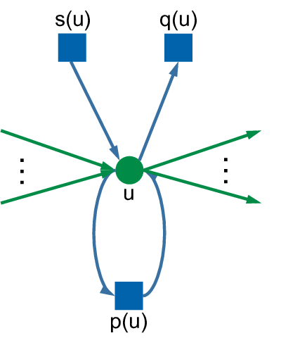
We formulate the NSDP as a MCCF problem on the cloud-augmented graph that results from augmenting each node in $\mathcal{G}$ with the gadget in Fig. 2, where $p(u),s(u)$, and $q(u)$ denote the processing unit, source unit, and demand unit at cloud node $u$, respectively. The resulting graph is denoted by $\mathcal{G}^{a}=(\mathcal{V}^{a},\mathcal{E}^{a})$, with $\mathcal{V}^{a}=\mathcal{V}\cup\mathcal{V}^{\prime}$, $\mathcal{E}^{a}=\mathcal{E}\cup\mathcal{E}^{\prime}$, and where $\mathcal{V}^{\prime}$ and $\mathcal{E}^{\prime}$ denote the set of processing, source, and demand unit nodes and edges, respectively. We denote by $\delta^{-}(u)$ and $\delta^{+}(u)$ the set of incoming and outgoing neighbors of node $u$ in $\mathcal{G}^{a}$.

In the cloud-augmented graph $\mathcal{G}^{a}$, each edge $(u,v)\in\mathcal{E}^{a}$ has an associated capacity, unit resource cost, and per-function resource requirement, as described in the following.

For the set of edges $\{(u,p(u)),(p(u),u):u\in\mathcal{V}\}$ representing the set of compute resources, we have:

• •

  $c_{u,p(u)}=c_{u}$, $c_{p(u),u}=c_{u}^{max}$

• •

  $w_{u,p(u)}=w_{u}$, $w_{p(u),u}=0$

• •

  $r^{(\phi,i)}_{u,p(u)}=r^{(\phi,i)}_{u},\forall(\phi,i)$

where $c_{u}^{max}=\sum_{(d,\phi,i)}\sum_{s\in\mathcal{S}(d,\phi)}\lambda_{s}^{(d,\phi)}r_{u}^{(\phi,i)}$. Note that we model the processing of network flows and associated allocation of compute resources using link $(u,p(u))$, and let edge $(p(u),u)$ be a free-cost edge of sufficiently high capacity that carries the processed flow back to node $u$.

For the set of edges $\{(s(u),u),(u,s(u)):u\in\mathcal{V}\}$ representing the resources via which client flows enter and exit the cloud network, we have:

• •

  $c_{s(u),u}=c_{u}^{max}$, $c_{u,q(u)}=c_{u}^{max}$

• •

  $w_{s(u),u}=0$, $w_{u,q(u)}=0$

• •

  $r^{(\phi,i)}_{s(u),u}=r^{(\phi,i)}_{u,q(u)}=0,\forall(\phi,i)$

Note that we model the ingress and egress of network flows via free-cost edges of sufficiently high capacity. In addition, the irrelevant per-function resource requirement for these edges is set to zero.

Given that the set of network resources only perform the fundamental transport function of moving bits between cloud network nodes, the per-function resource requirement for the set of edges in the original graph $(u,v)\in\mathcal{E}$ is set to $r^{tr}_{uv}$ for all $(\phi,i)$, i.e., $r^{(\phi,i)}_{uv}=r^{tr}_{uv},\forall(\phi,i)$. The capacity and unit resource cost of network edge $(u,v)\in\mathcal{E}$ is given by $c_{uv}$ and $w_{uv}$, respectively.

We now define the following MCCF flow and resource allocation variables on the cloud-augmented graph $\mathcal{G}^{a}$:

• •

  Flow variables: $f^{(d,\phi,i)}_{uv}$ indicates the fraction of commodity $(d,\phi,i)$ on edge $(u,v)\in\mathcal{E}^{a}$, i.e., the fraction of flow output of function $(\phi,i)$ for destination $d$ carried/processed by edge $(u,v)$.

• •

  Resource variables: $y_{uv}$ indicates the total amount of resource units (e.g., cloud or network resource units) allocated on edge $(u,v)\in\mathcal{E}^{a}$.

The NSDP can then be formulated via the following compact linear program:

where, when not specified for compactness, $u\in\mathcal{V}$, $d\in\mathcal{V}$, $\phi\in\Phi$, $i\in\{1,\dots,M_{\phi}\}$, and $(u,v)\in\mathcal{E}^{a}$.

The objective is to minimize the overall cloud network resource cost, described by (1a). Recall that the set $\mathcal{E}^{a}$ contains all edges in the augmented graph $\mathcal{G}^{a}$, representing both cloud and network resources. Eq. (1b) describes standard flow conservation constraints applied to all nodes in $\mathcal{V}$. A specially critical set of constraints are the service chaining constraints described by (1c). These constraints establish that in order to have flow of a given commodity $(d,\phi,i)$ coming out of a processing unit, the input commodity $(d,\phi,i-1)$ must be entering the processing unit. Constraints (1d) make sure that the total flow at a given cloud network resource is covered by enough resource units without violating capacity.¹¹ 1 Recall from the MCCF model that commodity $(d,\phi,i)$ gets processed by function $(\phi,i+1)$, and that $r^{(\phi,i)}_{uv}=r^{tr}_{uv},\forall(u,v)\in\mathcal{E},\phi,i$. Eqs. (1e) and (1f) establish the source and demand constraints. Note from (1f) that no flows of final commodity $(d,\phi,M_{\phi})$ are allowed to exit the network other than at the destination node $d$. Finally, (1g) describe the fractional and integer nature of flow and resource allocation variables, respectively.

In this work, we always assume fractional flow variables in order to capture the ability to split client flows to improve overall cloud network resource utilization. With respect to the resource allocation variables, however, we are interested in the following two main versions of the NSDP:

• •

  Integer NSDP: The use of integer resource variables allows accurately capturing the allocation of an integer number of general purpose resource units (e.g., servers). In this case, the NSDP becomes a generalization of multi-commodity network design (MCND), where the network is augmented with compute edges that model the processing of service flows and where there are additional service chaining constraints that make sure flows follow service functions in the appropriate order. In fact, for the special case that each service is composed of a single commodity, the NSDP is equivalent to the MCND. We refer to the resulting MCCND problem as the integer NSDP.

• •

  Fractional NSDP: The use of fractional resource variables becomes a specially good compromise between accuracy and tractability when the size of the cloud network resource units is much smaller than the total flow served at a given location. This is indeed the case for services that serve a large number of large-size flows (e.g., telco services [1]) and/or services deployed using small-size resource units (e.g., micro-services [10]). In this case, the NSDP becomes a generalization of min-cost MCF, with the exact equivalence holding in the case of single commodity services. We refer to the resulting MCCF problem as the fractional NSDP.

As discussed in the previous section, the fractional NSDP can be formulated as the MCCF problem that results from the linear relaxation of (1), i.e., by replacing $y_{uv}\in\mathbb{Z}^{+}$ with $y_{uv}\geq 0$ in (1g). While the resulting linear programming formulation admits optimal polynomial-time solutions, it requires solving a linear program with a large number of constraints. In this work, we are interested in designing a fast fully polynomial approximation scheme (FPTAS) for the fractional NSDP. A natural direction would be to build on state of the art FPTAS for MCF that rely on shortest-path computations [6, 8]. However, these techniques have only been shown to provide $O(\epsilon)$ approximations in time $O(1/\epsilon^{2})$. Here, we target the design of faster approximations with order improvements in running time, i.e., $O(1/\epsilon)$ and $O(1/\sqrt{\epsilon})$, by redesigning queue-length based algorithms that have been shown to be very effective for stochastic network optimization, in order to construct fast iterative algorithms for static MCCF problems such as the fractional NSDP.

It is immediate to show that the integer NSDP is NP-Hard by reduction from MCND. Recall that the integer NSDP is equivalent to MCND for the special case of single-commodity services. Hence, no $O(\epsilon)$ approximation can in general be computed in sub-exponential time. After recognizing the difficulty of approximating the integer NSDP, we now establish key observations on the behavior of QNSD that allows us to add a simple, yet effective, condition on the evolution of QNSD that enables constructing a solution to the integer NSDP of good practical performance.

We first observe that the QNSD algorithm evolves by allocating an integer number of resources in each iteration. In fact, QNSD solves a max-weight problem in each iteration and allocates either zero or the maximum number of resource units to a single commodity at each cloud network location. However, the solution in each iteration may significantly violate flow conservation constraints. On the other hand, the average over the iterations is shown to converge to a feasible, but, in general, fractional solution. Based on these observations, we propose C-QNSD (constrained QNSD), a variation of QNSD designed to constrain the solution over the algorithm iterations to satisfy flow conservation across consecutive iterations, such that when the iterative flow solution converges, we can guarantee a feasible solution to the integer NSDP. C-QNSD works just as QNSD, but with the max-weight problems solved in each iteration replaced by the fractional knapsak problems that result from adding the conditional flow conservation constraints:

Specifically, in each iteration of the main procedure, after the queue updates described by (3)-(5), the transport and processing decisions are jointly determined as follows:

• •

  Transport and processing decisions: For each $u\in\mathcal{V}$:

  		max		$\displaystyle\!\!\!\!\sum_{v\in\delta^{\!+\!}(u)}\sum_{(d,\phi,i)}W^{(d,\phi,i)}_{uv}f^{(d,\phi,i)}_{uv}(t)-Vy_{uv}(t)w_{uv}$
  		s.t.		$\displaystyle\!\!\!\eqref{cond},\eqref{cap},\eqref{vars}$
  		where
  		$\displaystyle\!\!\!\!\!\!W_{uv}^{(d,\phi,i)}(t)=\frac{1}{r_{uv}^{tr}}\left(U_{u}^{(d,\phi,i)}(t)-U_{v}^{(d,\phi,i)}(t)\right)$
  		$\displaystyle\qquad\qquad\qquad\qquad\qquad\qquad\forall v\in\delta^{\!+\!}(u)\backslash\{p(u)\}$
  		$\displaystyle\!\!\!\!\!\!W_{u,p(u)}^{(d,\phi,i)}(t)=\frac{1}{r_{u}^{(\phi,i\!+\!1)}}\left(U_{u}^{(d,\phi,i)}(t)-U_{u}^{(d,\phi,i\!+\!1)}(t)\right)$

Observe that without the conditional flow conservation constraints (11), the problem above can be decoupled into the set of max-weight problems whose solutions drive the resource allocation and flow rate assignment of QNSD. When including (11), the solution to the above maximization problem is forced to fill-up the cloud network resource units with multiple commodities, smoothing the evolution towards a feasible integer solution. In C-QNSD, the above maximization problem is solved via a linear-time heuristic that decouples the problem into a set of fractional knapsacks, one for each neighbor node $v\in\delta^{\!+\!}(u)$ and resource allocation choice $y_{uv}\in\{0,1,\dots,c_{uv}\}$.

As shown in the following section, C-QNSD effectively consolidates service flows into a limited number of active resources. Providing some form of performance guarantee is of interest to the authors, but out of the scope of this paper.

In this section, we evaluate the performance of QNSD and C-QNSD in the context of Abilene US continental network, composed of $11$ nodes and $28$ directed links, as illustrated in Fig. 3. We assume each node and link is equipped with $10$ cloud resource units and $10$ network resource units, respectively. The cost per cloud resource unit is set to $1$ at nodes $5$ and $6$, and to $3$ at all other nodes. The cost per network resource unit is set to $1$ for all $28$ links.

While not included in this paper for ease of exposition, our model and algorithms can be extended to include:

• •

  Function availability: Limiting the availability of certain functions to a subset of cloud nodes can be modeled by setting the flow variables associated with function $(\phi,i)$ to zero, $f^{(d,\phi,i)}_{p(u),u}=0$, for all $d$ and for all cloud nodes $u$ in which function $(\phi,i)$ is not available.

• •

  Function flow scaling: Capturing the fact that flows can change size as they go through certain functions can be modeled by letting $\xi^{(\phi,i)}$ denote the number of output flow units per input flow unit of function $(\phi,i)$, and modifying the service chaining constraints (1c) as $\xi^{(\phi,i)}f_{p(u),u}^{(d,\phi,i)}=f_{u,p(u)}^{(d,\phi,i-1)}$.

• •

  Per-function resource costs: If the cost function depends on the number of virtual resource units (e.g., VMs) instead of on the number of physical resource units (e.g., servers), then we can use $y^{(\phi,i)}_{uv}$ and $w^{(\phi,i)}_{uv}$ to denote the number of allocated resource units of function $(\phi,i)$ and the cost per resource unit of function $(\phi,i)$, respectively.

• •

  Nonlinear cost function: In order to capture nonlinear cost effects such as economies of scale in which the cost per resource unit decreases with the number of allocated resource units, the cost function can be modified as $\sum_{uv}y_{uv,k}w_{uv,k}$, with $y_{uv,k}\in\{0,1\}$ indicating the allocation of $k$ resource units, and $w_{uv,k}$ denoting the cost associated with the allocation of $k$ resource units. The capacity constraints in (1d) become $\sum_{(d,\phi,i)}\!f_{uv}^{(d,\phi,i)}r^{(\phi,i+1)}_{uv}\!\leq k\,y_{uv,k}\!\leq c_{uv}$.

We have formulated the NFV service distribution problem (NSDP) as a multi-commodity-chain network design problem on a cloud-augmented graph. We have shown that under load-proportional costs, the resulting fractional NSDP becomes a multi-commodity-chain network flow problem that admits optimal polynomial time solutions, and have designed QNSD, a queue-length based iterative algorithm that provides an $O(\epsilon)$ approximation in time $O(1/\epsilon)$. We further conjectured that, by exploiting the momentum obtained when combining differential queue backlogs across consecutive iterations, QNSD converges in time $O(1/\sqrt{\epsilon})$, and illustrated it via simulations. We then addressed the case in which resource costs are a function of the integer number of allocated resources. We showed that the integer NSDP is NP-Hard by reduction from MCND and designed C-QNSD, a heuristic algorithm that constrains the evolution of QNSD to effectively consolidate flows into a limited number of active resources.

Let

denote the matrix form of the QNSD queuing dynamics given by (3), where ${\bf f}(t)$, ${\bf Q}(t)$, and $\bf A$ denote the flow vector in iteration $t$, the queue-length vector in iteration $t$, and the matrix of flow coefficients, respectively.

Let

denote the dual function of the fractional NSDP weighted by the control parameter $V$, where ${\bf w}$ is the resource cost vector and $\mathcal{X}$ is the set of feasible solutions to the fractional NSDP.

Let $\mathcal{H}^{*}\triangleq\{{\bf Q}^{*}\!:\,\,{\bf Q}^{*}=\arg\max_{{\bf Q}}Z({\bf Q})\}$ denote the set of all optimizers of $Z({\bf Q})$.

Let $\mathcal{H}_{\gamma}\triangleq\left\{{\bf Q}:\sup_{{\bf Q}^{*}\in\mathcal{H}^{*}}\{\|{\bf Q}-{\bf Q}^{*}\|\}\leq\gamma\right\}$ denote the set of queue-length vectors that are at most $\gamma$-away from any point in $\mathcal{H}^{*}$. We further assume that the value of $\gamma$ is independent of the control parameter $V$.³³ 3 While we conjecture that this assumption is not needed to prove Theorem 1, it is technically needed for the type of proof used in this paper.

Since $Z({\bf Q})$ is a piecewise linear concave function of ${\bf Q}$, the locally polyhedron property is satisfied, i.e., : $\forall{\bf Q}\notin\mathcal{H}_{\gamma}$ and $\forall{\bf Q}^{*}\in{\mathcal{H}}^{*}$, there exists a $L_{\gamma}>0$ such that

We then denote the set of queue-length vectors that are $D$-away from $H^{*}$ as

with $D\triangleq\max\left\{\frac{B}{L_{\gamma}}-\frac{L_{\gamma}}{4},\frac{L_{\gamma}}{2},\gamma\right\}$ ,where $B$ is an upper bound for $\|{\bf A}{\bf f}\|^{2}$ defined as

We now state and prove the following lemmas, which are used to prove Theorem 1.

References

- [1] “Network Functions Virtualization: An Introduction, Benefits, Enablers, Challenges and Call for Action,” ETSI, White Paper, October 2012.
- [2] “Software-Defined Networking: The New Norm for Networks,” Open Networking Foundation, April 2012.
- [3] Bell Labs Strategic White Paper, “The Programmable Cloud Network - A Primer on SDN and NFV,” June 2013.
- [4] R. Cohen, L. Lewin-Eytan, J. Naor, D. Raz, “Near Optimal Placement of Virtual Network Functions,” IEEE INFOCOM, April 2015.
- [5] M. Barcelo, J. Llorca, A. M. Tulino, N. Raman, “The Cloud Servide Distribution Problem in Distributed Cloud Networks,” IEEE ICC, June 2015.
- [6] N. Garg, J. Konemann, “Faster and Simpler Algorithms for Multicommodity Flow and Other Fractional Packing Problems,” SIAM Journal on Computing, May 2007.
- [7] D. Bienstock, G. Iyengar, “Approximating Fractional Packings and Coverings in O(1/epsilon) Iterations,” SIAM Journal on Computing, July 2006.
- [8] Z. Cao, M. Kodialam, T. V. Lakshman, “Traffic Steering in Software Defined Networks: Planning and Online Routing,” ACM SIGCOMM Computer Communication Review, vol. 44, no. 4, August 2014.
- [9] T. G. Crainic, A. Frangioni, B. Gendron, “Bundle-based Relaxation Methods for Multicommodity Capacitated Fixed Charge Network Design,” Discrete Applied Mathematics, vol. 112, pp. 73-99, 2001.
- [10] N. Dragoni, S. Giallorenzo, A. L. Lafuente, M. Mazzara, F. Montesi, Ruslan Mustafin, Larisa Safina, “Microservices: Yesterday, Today, and Tomorrow,” arxiv, June 2016.
- [11] H. Feng, J. Llorca, A. M. Tulino, A. F. Molisch, “Dynamic Service Optimization in Distributed Cloud Networks,” IEEE INFOCOM SWFAN Workshop, April 2016.
- [12] S. Supittayapornpong, L. Huang, M. J. Neely, “Time-average Stochastic Optimization with Non-Convex Decision Set and its Convergence,” IEEE CDC, December 2014.
- [13] P. Tseng, “On Accelerated Proximal Gradient Methods for Convex-Concave Optimization,” SIAM Journal on Optimization, May 2008.
- [14] J. Liu, A. Eryilmaz, N. B. Shroff, E. S. Bentley, “Heavy-Ball: A New Approach to Tame Delay and Convergence in Wireless Network Optimization,” IEEE INFOCOM, April 2016.
- [15] D. P. Bertsekas, “Convex Optimization Theory,” Belmont: Athena Scientific, pp. 157-226, 2009.