Data-driven discovery of interpretable causal relations for deep learning material laws with uncertainty propagation
Abstract
This paper presents a computational framework that generates ensemble predictive mechanics models with uncertainty quantification (UQ). We first develop a causal discovery algorithm to infer causal relations among time-history data measured during each representative volume element (RVE) simulation through a directed acyclic graph (DAG). With multiple plausible sets of causal relationships estimated from multiple RVE simulations, the predictions are propagated in the derived causal graph while using a deep neural network equipped with dropout layers as a Bayesian approximation for uncertainty quantification. We select two representative numerical examples (traction-separation laws for frictional interfaces, elastoplasticity models for granular assembles) to examine the accuracy and robustness of the proposed causal discovery method for the common material law predictions in civil engineering applications.
1 Introduction
Computer simulations for mechanics problems often require material (constitutive) laws that replicate the local constitutive responses of the materials. These material laws can be used to replicate the responses of an interface (e.g., traction-separation laws or cohesive zone models) or bulk materials (e.g., elastoplasticity models for solids, porosity-permeability relationship and water retention curve). A computer model is then completed by incorporating these local constitutive laws into a discretized form of balance principles (balance of mass, linear momentum and energy) where discretized numerical solutions can be sought by a proper solver.
Constitutive laws, such as stress-strain relationship for bulk materials, traction-separation laws for interface, porosity-permeability for porous media, are often derived following a set of axioms and rules (Truesdell and Noll 2004). In these hand-crafted models, phenomenological observations are incorporated into constitutive laws (e.g., critical state theory for soil mechanics (Schofield and Wroth 1968; Sun 2013; Bryant and Sun 2019; Na et al. 2019), void-growth theory for ductile damage (Gurson 1977)). While the earlier simpler models are often amended by newer and more comprehensive models (Dafalias 1984) in order to improve the performance (e.g. accuracy, more realistic interpretation of mechanisms), these improvements are often a trade-off that may unavoidably increase the number of parameters, leading to increasing difficulty for the calibration, verification and validation processes, as well as the uncertainty quantification (Dafalias 1984; Borja and Sun 2007; Borja and Sun 2008; Clément et al. 2013; Wang and Sun 2019a; Wang et al. 2016).
The rise of big data and the great promises of machine learning have led to a new generation of approaches that either bypass the usages of constitutive laws via model-free data-driven methods (e.g., Kirchdoerfer and Ortiz 2016; He and Chen 2020; Bahmani and Sun 2021; Karapiperis et al. 2021) or replace parts of the modeling efforts/components with models generated from supervised learning (e.g., Furukawa and Yagawa 1998; Lefik and Schrefler 2003; Wang and Sun 2018; Wang and Sun 2019b; Zhang et al. 2020; Vlassis et al. 2020a; Vlassis and Sun 2021; Logarzo et al. 2021; Masi et al. 2021). However, one critical issue of these machine learning and data-driven approaches is the lack of sufficient interpretability of predictions. While there is no universally accepted definition of interpretability, we will herein employ the definition used in Miller 2019 which refers interpretability as the degree to which a human can understand the cause of the prediction.
One possible way to boost the interpretability is to introduce a proper medium to represent knowledge that can be understood by human (Sussillo and Barak 2013). Causal graph, also known as causal Bayesian network, is one such medium in which the causal relations among different entities are mathematically represented by a directed graph. In the application of computational mechanics Wang and Sun 2018; Wang and Sun 2019b; Heider et al. 2020 have derived a mathematical framework to decompose a complex prediction task into multiple easier predictions represented by subgraphs within graphs. More recent work such as Wang and Sun 2019a; Wang et al. 2019 introduce a deep reinforcement learning approach that employs the Monte Carlo Tree Search (MCTS) to assemble a directed graph that generates a sequence of interconnected predictions of physical quantities to emulate a hand-crafted constitutive law. However, these directed graphs are generated to optimize a given performance metric (e.g. accuracy, calculation speed and forward prediction robustness), but not necessarily reveal the underlying causal relations among physical quantities.
Discovering causal relations from observational data is an important problem with applications in many fields of science, such as social science (Oktay et al. 2010), finance (Gong et al. 2017), and biomedicine (Shen et al. 2020). The standard way to discover causality is through randomized controlled experiments. However, conducting such experiments can be either impractical, unethical, and/or very expensive in many disciplines (Xu et al. 2012; Xie and Xu 2020). For mechanics problems, the major issues include the time and labor cost for physical experiments, the lack of facilities or equipment to complete the required tests and the difficulties to obtain specimens (Mitchell et al. 2005; Powrie 2018; Wood 1990). As a result, an alternative approach, which is adopted in this study, is to use sub-scale simulations as the digital representation that generates auxiliary data sets to build material laws or forecast engine for the macroscopic material responses (Liu et al. 2016; Ma and Sun 2020; Frankel et al. 2019; Wang and Sun 2019b). Classic methods for causal discovery are based on probabilistic graphical modeling (Pearl 2000), the structure of which is a directed acyclic graph (DAG) with nodes representing random variables and edges representing conditional dependencies between variables. Learning a DAG from observational data is highly challenging since the number of possible DAGs is super-exponential to the number of nodes. There are two main approaches for causal discovery: the constraint-based approach and the score-based approach. The constraint-based approach aims to recover a Markov equivalence class through inferring conditional independence relationships among the variables, and the resulting Markov equivalence class may contain multiple DAGs that indicate the same conditional independence relationships (Le et al. 2016; Cui et al. 2016). On the other hand, the score-based approach uses a scoring function, such as the Bayesian Information Criterion (BIC), to search for the DAG that best fits the data (Heckerman et al. 1995; Huang et al. 2018).
In this paper, we aim to discover causal relations that can explain the underlying mechanism of a history-dependent macroscopic constitutive law upscaled from direct numerical simulations at the meso-scale. The most common method for constructing the causal relations from time-series data is Granger causality (Granger 1969), which assumes a number of lagged effects and analyzes the data in a unit no more than that number of lags. See Runge 2018 for a review of causal discovery methods on time-series data. However, most of these causal discovery methods assume that the data are generated from a stationary process, meaning that the data are generated by a distribution that does not change with time. Such an assumption does not hold in many physical processes, in which the mechanisms or parameters in the causal model may change over time. Several methods have been proposed recently to tackle time-varying causal relations in non-stationary processes (Ghassami et al. 2018; Huang et al. 2019a; Huang et al. 2020). However, they either assume linear causal models, or does not offer the flexibility of incorporating known physical knowledge, limiting their applicability to the nonlinear path-dependent relations in learning material constitutive laws.
In this work, we offer two major innovations. First, we introduce a new decoupled discovery/training approach where the discovery of causal relations represented by a DAG is enabled by a causal discovery algorithm that deduces plausible causal relations from non-stationary time series data and incorporates known physical knowledge. Second, we leverage the obtained causal graph as the representation of mechanics knowledge and adopt a Bayesian approximation using the dropout layer technique first introduced by Gal and Ghahramani 2016a to propagate epistemic uncertainty in the causal graph and generate quantitative predictions with uncertainty quantification.
The rest of the paper is organized as follows. Section 2 first introduces the two data sets (learning traction-separation law and hypo-plasticity of granular materials) used for our numerical experiments. This is followed by the description of theory and implementation of the proposed causal discovery algorithm used to deduce the causal relations from non-stationary time series data (Section 3). The setup of the deep neural network model for the prediction tasks and the uncertainty propagation are included in Sections 4 and 5 respectively. The proposed framework is then tested against two numerical experiments (Section 6), which is then followed by the conclusion.
2 Causal relations and constitutive laws
As demonstrated in previous studies such as Wang and Sun 2018; Wang and Sun 2019a; Wang and Sun 2019b; Wang et al. 2019; Heider et al. 2020; Vlassis et al. 2020a, the relationships in a constitutive model can be represented by a network of unidirectional information flow, i.e., a DAG where represents a vertex set and denotes an edge set. With appropriate assumptions that will be discussed later, the DAG can be identified as a causal graph (Pearl 2000). The causal relations are not only useful to explain the underlying mechanism of a process but also provide us a basis to formulate multi-step transfer learning to predict constitutive responses. This strategy can be beneficial because one can leverage more data gathered from physical numerical experiments to train the prediction model. For instance, while a black-box prediction of stress-strain curves only leverages the stress-strain pair for supervised learning, the introduction of knowledge graphs may introduce multiple supervised learning tasks where measurements of porosity, fabric tensors or any other physical and geometrical attributes measured during the experiments can be leveraged to improve the training. For completeness, we briefly describe the procedure to consider the data set as vertex sets in graphs and the causal discovery process used to create the directed edge set in a knowledge graph through two examples.
Note that many of the physical quantities that become the vertices in the knowledge graphs are graph metrics obtained from analyzing the connectivity topology of the granular system. For brevity, we will not provide a review on the applications of graph theory for granular matter here. Interested readers may refer to Appendix B for the definitions of the graph metrics and Satake 1978; Bagi 1996; Walker and Tordesillas 2010; Tordesillas et al. 2010; O’Sullivan 2011; Kuhn et al. 2015 and Vlassis et al. 2020a for reviews on the graph theory applied to particulate and granular systems.
2.1 Dataset for traction-separation law
In the first example, our goal is to conduct a numerical experiment to verify whether the causal discovery algorithm is able to re-discover the well-known causal relation that links the plastic dilatancy and contraction to the frictional behaviors (Scholz 1998; Popov 2010) with a small data set.
Following Wang and Sun 2018; Wang and Sun 2019a; Wang and Sun 2019b; Wang et al. 2019, we consider the vertex set consists of five elements, the displacement jump/separation , the traction , and three geometric measures, i.e.,
- 1.
Displacement jump , the relative displacement of an interface of two in-contact bodies.
- 2.
Porosity , the ratio between the volume of the void and the total volume of RVE.
- 3.
Coordination number (averaged) where is the number of particle contacts and is the number of particles in the RVE.
- 4.
Fabric tensor where is the normal vector of a particle contact in the RVE. The symbol ‘’ denotes a juxtaposition of two vectors (e.g., ) or two symmetric second order tensors [e.g., ].
- 5.
Traction , the traction vector acts on the interface.
To generate a machine learning based traction-separation law, we identify the displacement jump as the root and the traction as the leaf of the causal graph. The causal graph is a DAG where is the set consisting of the physical quantities and . Meanwhile, is a set of directed edges that connect any two elements from , and is determined from the causal discovery algorithm outlined in Section 3.
The dataset is generated using an open-source code YADE. In total, there are 100 traction-separation law simulations run with different loading paths performed on the same RVE. This RVE consists of spherical particles with radii between mm with uniform distribution. The RVE has a height of 20 mm in the normal direction of the frictional surface and is initially consolidated to an isotropic pressure of 10 MPa. The inter-particle interaction is controlled by Cundall’s elastic-frictional contact model (Cundall and Strack 1979) with an inter-particle elastic modulus of , a ratio between shear and normal stiffness of , a frictional angle of , a density , and a Cundall damping coefficient . For brevity, the generation and setup of the simulations are not included in this paper. Interested readers please refer to Wang and Sun 2019a for more information. The data required to replicate the results of this paper and for 3rd-party validation can be found in the Mendeley Data repository (Sun and Wang 2019).
2.2 Dataset for hypo-plasticity of granular materials
While the first data set is used to determine whether the causal graph algorithm may re-discover known physical relations in the literature, the second problem is designed to test whether the causal graph algorithm may successfully investigate new plausible causal relations not known a prior in the literature.
For this purpose, we run 60 discrete element simulations and use 30 of them for calibrations and 30 for blind forward predictions. In addition to the conventional microstructural attributes (e.g., porosity and fabric tensor) typically used for hand-crafted constitutive laws (Manzari and Dafalias 1997; Dafalias and Manzari 2004; Sun 2013; Bryant and Sun 2019; Na et al. 2019), we have also recorded the evolution of the particle contact pairs in each incremental time step of the discrete element simulations. The particle contact connectivity is itself an undirected graph where is the set of particles and is the set of particle contacts, one for each contact between two contacting convex particle represented. They are undirected edges. To facilitate new discovery, we compute 15 different graph metrics of (see Appendix B for definition) that have not been used for composing constitutive laws and see if (1) whether the causal discovery algorithm may discover causal relations among these new physical quantities and (2) whether the new discovery helps improve the accuracy, robustness and consistency of the forward predictions enabled by neural networks trained according to the discovered causal relations.
In total, there are 11 types of time-history data in which 3 of them are second-order tensors (strain, stress and the strong fabric tensor), and the rest are scalar (porosity, coordination number graph density, graph local efficiency, graph average clustering, graph degree assortativity coefficient, graph transitivity and graph clique number). As such there are 11 elements in the vertex set and the goal of the causal discovery is to establish the edge set to complete the causal graph. A sequence of supervised learning is then used to generate predictions via deep learning.
3 Causal discovery and knowledge graph constructions
3.1 Notations and assumptions
Let be a DAG containing only directed edges and has no directed cycles. For each , let denotes the set of parents of in . Since our data are time-history dependent, we assume that the joint probability distribution of at each time point according to can factorize as where is the number of vertices in . Here can be regarded as “causal mechanism.” For non-stationary time series data, the causal mechanism can change over time, and the changes may be due to the involved functional models or the causal strengths.
Throughout this section, we use the example of traction-separation law to illustrate the proposed causal discovery method without loss of generality. Therefore, is the set consisting of displacement jump , porosity , coordination number , fabric tensor , and traction . Huang et al. 2019b developed a constraint-based causal discovery algorithm for non-stationary time series data to identify changing causal modules and recover the causal structure. In this paper, we extend the algorithm in Huang et al. 2019b such that the proposed causal discovery algorithm not only handles non-stationary time-history data but also incorporates certain physical constraints. For example, in constructing the traction-separation law, we have the prior knowledge that the dynamic changes in can cause changes in other variables, not vice versa. Therefore, if there exists a directed edge between the displacement jump and any other variable , then .
Denote to include all other variables in excluding (e.g., porosity, fabric tensor). Since the causal mechanism can change over time, we assume that the changes can be explained by certain time-varying confounders, which can be written as functions of time. As we have the prior knowledge that itself is a time-dependent variable and could affect all other variables, we regard as such a confounder and assume that the causal relation for each can be represented by the following structural equation model:
| (1) |
where includes if the changes in can affect the changes in , denotes a function of that influences as effective parameters, is a noise term that is independent of and . The ’s are assumed to be independent. As we treat as a random variable, there is a joint distribution over . Denote to be the graph by adding to , and for each , adding an arrow from to . Note that is the induced subgraph of over . Denote the joint distribution of to be .
In order to apply any conditional independence test on the variable set for recovering causal structure, we set the following assumptions (Spirtes et al. 2000).
Assumption 1. (Causal Markov condition) and the joint distribution on satisfy the causal Markov condition if and only if a vertex of is probabilistically independent of all its non-descendants in given the set of all its parents.
Assumption 2. (Faithfulness) and the joint distribution satisfy the faithfulness condition if and only if no conditional independence holds unless entailed by the causal Markov condition.
Assumption 3. (Causal sufficiency) The common causes of all variables in are measured.
3.2 Recovery of the causal skeleton
In this section, we propose a constraint-based method building upon the PC algorithm (Spirtes et al. 2000) to first identify the skeleton of , defined as the obtained undirected graph if we ignore the directions of edges in a DAG . We prove that given Assumptions 1-3, we can apply conditional independence tests to to recover the skeleton of . Algorithm 1 describes the proposed method, which is supported by Theorem 1. The proof is provided in Appendix A following Huang et al. 2019b.
Theorem 1.
Given Assumptions 1-3, for every , and are not adjacent in if and only if they are independent conditional on some subset of .
In lines 3-7 of Algorithm 1, we determine whether the changes in cause changes in . If not, is not in the parent set of and there is no edge between and in . The lines 8-12 of Algorithm 1 aims to identify the causal skeleton between variables in except . Since how other variables change with and the relations between these variables are usually unknown and potentially very complex, we use a nonparametric conditional independence test, kernel-based condition independence (KCI) test developed by Zhang et al. 2012, to determine the dependence between variables throughout this paper. This nonparametric approach can not only capture the linear/nonlinear correlations between variables by testing for zero Hilbert-Schmidt norm of the partial cross-covariance operator, but also handle multidimensional data that are common in mechanics problems.
3.3 Determination of causal directions
After obtaining the skeleton , we need to determine the causal directions of edges. Meek 1995 provided a set of orientation rules to determine the directions of undirected edges in a graph based on conditional independence tests. However, the Meek rule (Meek 1995) is only applicable to edges that satisfy its conditions. In this section, we first introduce the Meek rule (Meek 1995), then propose an algorithm to orient the edges that are not covered by the Meek rule after incorporating known physical knowledge.
Denote to be an undirected edge. The Meek rule has the following principles:
- 1.
For all triples , if and are marginally independent but conditionally dependent given , then ;
- 2.
If and there is no edge between and , then orient ;
- 3.
If and there is an edge between and , then orient ;
- 4.
If , , and , then .
Now we describe our algorithm on how to determine the edge directions in the obtained skeleton . Firstly, for any node adjacent to , we orient due to the prior physical knowledge that only affects other variables, not vice versa. Then we apply the Meek rule to the obtained graph after orienting the edges from to its neighbours. For instance, suppose , if and are independent given a set of variables including , then we orient ; if and are independent given a set of variables excluding , then we have .
Next, we discuss how to determine the edge direction between two adjacent variables if they are both adjacent to , i.e., , , and , since such a scenario is not covered by the Meek rule. The modularity property of causal systems (Pearl 2000) demonstrated that if there are no confounders for cause and effect, then and are either fixed or change independently. Based on this principle, since both and change with , we can test the conditional independence between and , as well as between and to determine the direction between and . That says, if and are conditionally independent but and are not, then . Huang et al. 2019b developed a kernel embedding of non-stationary conditional distributions and extended the Hilbert Schmidt Independence Criterion (HSIC, Gretton et al. 2008) to measure the dependence between distributions, based on which the causal directions can be determined. For example, if we have two random variables and , we can compute the dependence between and using the normalized HSIC, denoted by . By the same token, we can compute the dependence between and using the normalized HSIC, denoted by . If , we orient ; otherwise . After orienting all possible edges, we can get the Markov equivalent class of the DAG . Algorithm 2 summarizes the proposed method on how to determine causal directions.
Remark 1.
In the numerical examples, we setup a threshold inclusion probability () below which the causality relation is not included in the hierarchical neural network models. This treatment allows us to ensure that the causalities with sufficient likelihoods are included but the less prominent relationship is omitted to improve the efficiency and simplicity of the resultant model. This threshold can be viewed as a hyperparameter. A highly threshold may yield a DAG with less vertices and therefore reduce the total number of required supervised training at the expense of being less precise on the causality relations among the data.
4 Supervised learning for path-dependent material laws
Once causal relations are identified, a directed graph can be established where there is an edge from the node to if is a direct cause of . Denote the leaf node to be the vertex that is not the cause to any other vertices, the root node to be the vertex that is not the target of any other vertices. Figure 1 demonstrates a directed graph indicating an information flow how leaf node(s) is related to root node(s) via some intermediate nodes, e.g., in Figure 1 , , and are sets of root, leaf, and intermediate nodes.
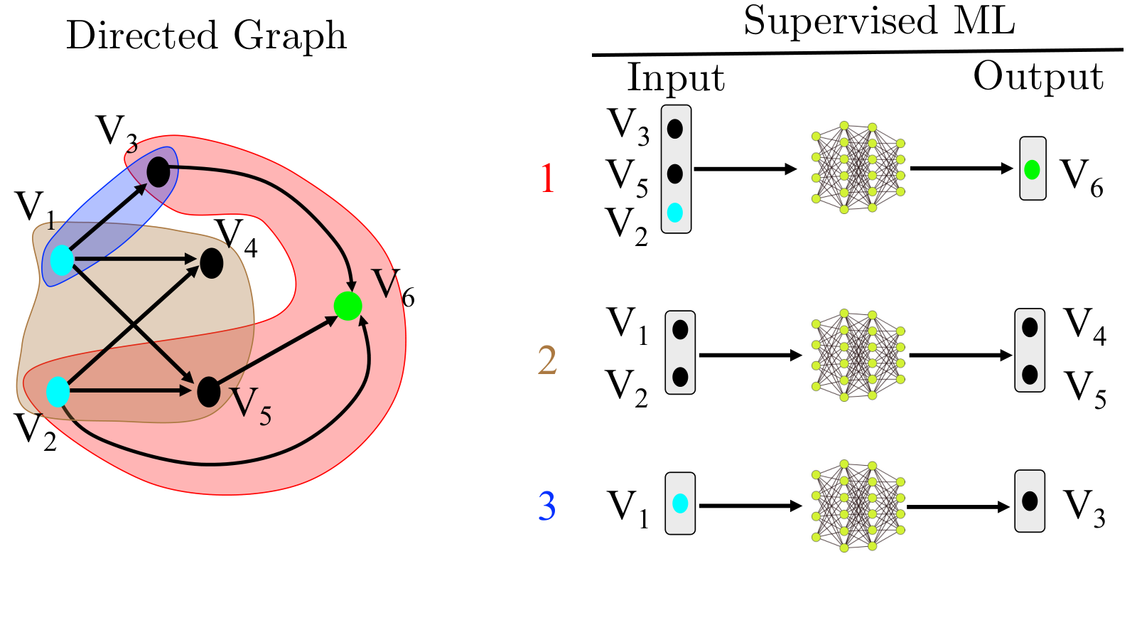
Along with the similar idea introduced in Wang and Sun 2019a, we aim to discover all sub-graphs that sequentially pass the information from the root to leaf, see Algorithm 3. Each of these subgraphs will contain leaf and root but without any intermediate nodes. As such, supervised learning can help us train neural network that predict the root of each subgraph with the corresponding leaf (or leaves) as input(s). To identify all sub-graphs, we traverse the graph backward from leaf to root nodes. The leaf with its immediate predecessors formed a directed tree which will be added into the list of potential sub-graphs. Then, we remove edges of the founded tree in the graph . In the next step, we select a new leaf node from the updated and do the process just described until there is not any edges in . For the case shown in Figure 1 we have the following potential sub-graphs:
| (2) | ||||
| (3) | ||||
| (4) | ||||
| (5) |
Those sub-graphs (directed trees) that share common upstream nodes will be merged into a bigger sub-graph. For the graph in Figure 1 final sub-graphs are:
| (6) | ||||
| (7) | ||||
| (8) |
For each sub-graph, we have a separate supervised machine learning (ML) task. In each ML task, inputs and outputs features are upstream and downstream nodes in each directed sub-graph, as shown in Figure 1(b).
In the training step, we use the same architecture for all ML tasks consisting of five layers GRU-Dropout-GRU-Dropout-Dense. Each GRU layer has 32 neurons, and the linear activation function is used for the Dense layer. Gated Recurrent Unit (GRU) is one type of Recurrent Neural Networks (RNN) to model history dependence (Chung et al. 2014). We use the GRU to strengthen the robustness of the ML black-box in dealing with any possible path-dependence (Wang et al. 2019). The dropout rate in the GRU is controlled to quantify uncertainty in the model prediction, which will be detailed in Section 5. All the input and output feature columns for each supervised learning task are normalized to zero mean and unity standard deviation. The loss function is defined as the mean squared root error between output prediction and ground truth. This loss is minimized by the Adam optimizer inside Keras library with Tensorflow 2.0 as its backend. Optimization process is done by the mini-batch stochastic gradient descent algorithm with a batch size 256 during 1000 epochs. The described neural network architecture and hyperparameters are chosen to be as close as possible to the ones used in Wang and Sun 2019a.
Note that, the tuning of the hyperparameters (e.g. number of neurons, number of layers, type of activation) may have a significant effect on the performance of the neural network models. The best combination of hyperparameters can be estimated via a variety of approaches such as the greedy search, random search (Bergstra and Bengio 2012), random forest (Probst et al. 2019), Bayesian optimization (Klein et al. 2017), meta-gradient iteration or deep reinforcement learning (Wang et al. 2020; Fuchs et al. 2021). In this work, we adopt the random search approach in Bergstra and Bengio 2012 to fine-tune the hyperparameters (cf. Sec. 6.1) A rigorous hyperparameter study that compares different hyperparameter tuning for neural networks that generates constitutive laws may provide further insights on the optimal setup of the hyperparameters but is out of the scope of this study.
For the blind prediction, after training, we start from the root (e.g., in the traction-separation law) and sequentially predict intermediate nodes via their corresponding sub-graph trained neural networks (NN) until reaching the leaf node. For example in the case shown in Figure 1: NN 3 predicts from input ; and are predicted by NN 2 from inputs and ; and finally NN 1 is used to predict the target variable from input and the obtained intermediate nodes and .
5 Uncertainty propagation in causal graph with dropout layers
As described in Section 4, we use the deep learning method, GRU in the training step and prediction to handle path-dependent predictions. However, the GRU itself is not designed to capture prediction uncertainty, which is of crucial importance in learning material law. In machine learning and statistics, Bayesian methods as probabilistic models provide us a natural way to quantify the model uncertainty through computing the posterior distribution of unknown parameters (Xie and Xu 2020). However, these methods often suffer from a prohibitively high computational cost. In this paper, we show that the dropout technique (Srivastava et al. 2014) used in the GRU can quantify uncertainty in prediction as a Bayesian approximation.
Dropout, a regularization method that randomly masks or ignores neurons during training, has been widely used in many deep learning models to avoid over-fitting and improve prediction (Hinton et al. 2012; Li et al. 2016; Boluki et al. 2020). Gal and Ghahramani 2016a firstly prove the link between dropout and a well known probabilistic model, the Gaussian process (Rasmussen 2003), and show that the use of dropout in the feed forward neural networks can be interpreted as a Bayesian approximation of Gaussian processes. In the context of RNNs, Gal and Ghahramani 2016b treated RNNs as probabilistic models by assuming network weights as random variables with a Gaussian mixture prior (with one component fixed at zero with a small variance). Such a technique is similar to the spike-and-slab prior in Bayesian statistics for variable selection (Ishwaran et al. 2005). Then Gal and Ghahramani 2016b show that optimizing the objective in the variational inference (Blei et al. 2017) for approximating the posterior distribution over the weights is equivalent to conducting dropout in the respective RNNs, and demonstrate the implementation in one commonly-used RNN model, the long short-term memory (Hochreiter and Schmidhuber 1997). In this section, we propose to extend the technique developed in Gal and Ghahramani 2016b in the context of GRUs for uncertainty quantification (UQ) in the prediction.
Given training inputs and the corresponding output , suppose that we aim to predict an output for a new input . From the Bayesian point of view, the prediction uncertainty can be characterized by the posterior predictive distribution of as follows:
| (9) |
where includes all unknown model parameters, is the posterior distribution of . In the GRU, all unknown weights can be viewed as . As the posterior distribution is generally intractable, the variational inference method approximates it by proposing a variational distribution and then finding the optimal parameters in the variational distribution through minimizing the Kullback-Leibler (KL) divergence between the approximating distribution and the full posterior distribution:
| (10) |
where is the prior distribution of .
Given an input sequence of length , the hidden state at time step in the GRU neural network can be generated as follows:
| (11) | ||||
where denotes the sigmoid function and denotes the element-wise product. Also, we assume that the model output at time step can be written as . Then the unknown parameters in the GRU are . We write and for the output in order to make the dependence on clear.
Then the right hand of (10) can be written as follows:
| (12) |
which can be approximated by Monte Carlo integration with the generated samples and plug in the sampled ’s to (12).
Following Gal and Ghahramani 2016b, we use a mixture of Gaussian distributions as the variational distribution for every weight matrix row :
| (13) |
where is the dropout probability, is the variational parameter (row vector), and is a small variance. We optimize over by minimizing the KL divergence in (12). Sampling each row of is equivalent to randomly mask rows in each weight matrix, i.e., conducting dropout. Then the predictive posterior distribution can be approximated by
| (14) |
where and is the total number of generated samples.
To implement the dropout in the GRU, we re-parametrize (11) as follows:
| (15) |
where and denote randomly masks repeated at all time steps.
We take the prediction tasks in Fig. 1 for example. The posterior predictive distribution of given is straightforward by (14) since only root and leaf nodes are involved. When involving the intermediate nodes, e.g., the subgroup , the posterior predictive distribution of given the root nodes ( and can be computed by
| (16) |
Specifically, when we generate samples from the posterior distribution of , we also generate samples for the intermediate nodes. Those samples of and the corresponding intermediate nodes can be then used in Monte Carlo integration to calculate (16). Throughout this paper, we set =200.
6 Numerical Examples
In this section, we conduct two numerical experiments to test our proposed framework that combines causal discovery with deep learning to build constitutive laws for granular materials. In Section 6.1, the causal discovery is conducted to determine the constitutive relationships for an RVE interface composed of spherical grains. The subsequent supervised machine learning then leverages the causal relations learned from the causal discovery algorithm to establish a serial of supervised learning that constitutes a forecast engine for traction. The propagation of uncertainty is enabled by the dropout technique that approximates Monte Carlo simulations to determine the confidence intervals for a given dropout rate. In Section 6.2, the same exercise is repeated for another data set to generate hypoplasticity surrogate model for a discrete element assembly where new topological measures are computed and incorporated into the proposed framework to (1) discover new physical mechanisms and (2) determine the benefit of the new discovery on the accuracy, robustness, and consistency of the forward predictions on unseen events.
6.1 Numerical Example 1: Machine Learning traction-separation law
Traction-separation laws are known as one of the main ingredients of cohesive fracture models used for brittle materials (Pandolfi et al. 2000; Park and Paulino 2011). Generally, a traction-separation law constitutes a relation between traction and displacement jump fields over the fracture surface. There exist many hand-crafted models developed by experts for different applications (Park and Paulino 2011), while no unified framework had been developed until recently by Wang and Sun 2019a who suggest an approach based on reinforcement learning. Also, in some applications such as granular materials more descriptors, e.g., porosity or fabric tensor, should be considered in these constitutive laws (Sun et al. 2013) to derive more predictive models. Lack of robustness in adding more descriptors is another weakness of classical models.
Our first test for the data-driven causal discovery model with dropout UQ is on the traction-separation law data publicly available in the repository Mendeley data (cf. Sun and Wang 2019). This dataset has also been used in Wang and Sun 2019a where the traction-separation law is determined from reinforcement learning. Our major point of departure is three-fold. Firstly, we develop a causal discovery algorithm to identify causal relations among history-dependent physical quantities in RVE simulations. Secondly, we decouple the causal discovery from the training of the neural network such that we now first discover causal relations, then utilize the discovered relationships to generate quantitative predictions using the method detailed in section 4. Thirdly, we introduce the Bayesian approximation using the dropout technique to propagate the uncertainty in the causal graph, building upon the theoretical framework established in Gal and Ghahramani 2016b.
The database includes 100 DEM experiments. In each DEM experiment, the time history of all the variables included in the DAG are recorded. Each experiment is conducted by a different ratio of normal to tangential loading rate and loading-unloading cycles on the same representative volume element of granular materials. As such, the total number of time-history data points in these experiments may vary from 51 to 111.
The interested reader is referred to the appendix in Wang and Sun 2019a for more information. In our study, feature space consists of displacement jump vector, traction vector, coordination number, symmetric part of fabric tensor, and porosity. We use half of the experiments for causal discovery and training artificial neural networks, and the rest is used for test and validation. In the causal discovery step, as different experimental setups may lead to different causal relations among variables, we apply the proposed causal discovery algorithm (Algorithms 1 and 2 in Section 3) to each of the training experiment, and then report the final causal graph by calculating the inclusion probabilities of directed edges appearing in all training experiments. The inclusion probability of one edge is defined as the proportion of causal graphs containing this edge. The directed edges with inclusion probabilities being larger than a pre-defined threshold (20% in our paper) are kept in the final causal graph. When both edge directions between two variables appear with positive inclusion probabilities (e.g., and both exist), we keep the edge direction that has a higher inclusion probability. The goal of the resultant model is to predict the same granular assembly responds to a different cyclic loading path unseen in the training. As such, the focus of this model is to generate a surrogate for one representative element volume.
Fig. 2 plots the final causal graph on the training data sets with edge inclusion probabilities. The strong confidence () in the edge starting from the displacement jump vector to porosity is consistent with the common field knowledge, i.e., the immediate consequence of displacement jump is the volume change.
The displacement jump vector, as the only control variable, affects all the intermediate physical quantities and traction vector. This observation may seem to be trivial, but it is not always the case which will be shown in the next example. The causal effects of fabric and coordination number on traction is aligned with the modern Critical State Theory (Li and Dafalias 2012) which is obtained without expert interpretation by the causal algorithm. Note that fabric encodes microstructural information in more detail such as directional dependence due to its tensorial nature, rather than porosity which smears out information into one scalar quantity. Therefore, it is reasonable to see that fabric has a considerable contribution in describing material behavior with a complex arrangement of force chains at the microstructural level.

Remark 2.
To make sure the suggested neural network architecture in Sec. 4 works satisfactorily in this problem, we trained several neural networks with different hyper-parameters for each sub-graph learning task in Fig. 2. We used the random search approach (Bergstra and Bengio 2012) implemented in Keras Tunner package (O’Malley et al. 2019) for this study. The number of GRU layers is kept fixed and equal to two, and in the training stage, the dropout rate is set to zero. The number of epochs is also set to 200. The parameters under this study are as follows: the number of units in GRU layers are sampled from the set , the Adam learning rate is sampled from the set , the batch size for the SGD algorithm is sampled from the set . Based on these hyperparameter ranges, each subgraph learning task has 240 different configurations; however, in the random search algorithm, we set the number of trials to 100 for each subgraph training task to reduce overall computational time. For this hyperparameter tuning task, we choose 50 data sets as the training set and another 50 data sets as the validation set. Our metric for selecting the best configuration is the minimum validation loss. We found that the learning rate 0.001 and batch size 32 are common among all the best configurations of subgraphs. In Table 1 we study the effect of number of units in GRU layers when learning rate and batch size have their optimal values.
| subgraph | mean | standard deviation | number of configurations | suggested NN |
|---|---|---|---|---|
| Porosity | 1.6e-6 | 7.36e-7 | 10 | 3.7e-6 |
| CN | 1.04e-3 | 2.3e-5 | 5 | 1.07e-3 |
| Fabric | 2.2e-3 | 3.98e-4 | 7 | 2.4e-3 |
| Traction | 5.1e-5 | 1.01e-5 | 8 | 9.1e-5 |
Applying Algorithm 3 to Fig. 2, we need to perform four supervised learning tasks: 1) predict Poro from the input ; 2) predict CN from the input and the intermediate node Poro; 3) predict fabric from the input and the intermediate nodes Poro and CN; and 4) predict the target variable from the input and the obtained intermediate nodes Poro, CN, and fabric. We then use the GRU to train each sub-graph with the dropout rate being 0.2 for both training and feed-forward predictions. Fig. 3 confirms that the neural network architecture proposed in section 4 yields satisfactory performance for all supervised tasks. To examine the generalization performance of the trained neural networks, we study the empirical cumulative distribution functions (eCDFs) for training and test data sets following Wang and Sun 2019a.
We define the point-wise scaled mean squared error (MSE) between a set of ground-truth values with size and its corresponding approximation set as:
| (17) |
where is a scaling function. In this paper, the scaling function linearly transforms a set of values into a new set where all values are in the range . We perform feed-forward predictions to obtain the distribution of each feature output at a specified load-step. For eCDF calculation only, we use the average of these predictions to approximate the feature output. In this way, the discrete eCDF of a target output feature, such as porosity, at data point is defined as where is the point-wise scaled MSE between the feature ground-truth value and its predictions’ average, is the total number of instances (i.e., the total number of data points across 50 training data sets) used for eCDF calculations, and is the indicator function. Fig. 4 plots eCDFs for all feature outputs in training and testing modes. In these plots, the eCDFs for test and training cases are almost the same, indicating no under-fitting or over-fitting issue exists. Note that the use of dropout in the GRU is not only for uncertainty quantification in prediction, but also to improve model generalization performance.
In the following, we present prediction results for one of the test cases where its applied normal and shear displacements are plotted in Fig. 5. Normal and shear displacement jumps experience cyclic loading-unloading path and are kept equal in magnitude.
We focus on the average of model predictions in Figs. 6 and 7. In Fig. 6, we see that the initial friction angle is close to degree which is almost half of the inter-particle friction angle. This reduction in the overall friction angle might be due to the induced dilation in the normal displacement. Another reason could be related to initial confining pressure: the higher the confining pressure is, the lower the friction angle is. In each loading-unloading branch, the behavior is almost linear without any energy dissipation, but further loading after a level makes the behavior nonlinear. If we only follow the loading path we observe the strain-softening which is the dominant mechanism of a dense granular assemblage; see Fig. 6 and 7(b). In other words, the material shows an unstable peak shear strength which is followed by a softening behavior until it reaches the critical state. The sign of changes in normal traction (Fig. 9(a)) and shear traction (Fig. 9(b)) are in agreement with the fabric normal (Fig. 10(a)) and shear (Fig. 10(b)) components, respectively. This confirms the tendency of fabric tensor to trace the load direction (Li and Li 2009; Li and Dafalias 2012; Wang and Sun 2016). Overall the proposed data-driven scheme can replicate main features of a realistic experiment, and there exists a good agreement between the model and experiment. However, there is an issue corresponding to second loading-unloading cycle where hysteresis is predicted by the model while experiment shows almost zero energy dissipation. This is mainly due to the neural network capacity and design and can be resolved by enriching the neural network architecture with wider neurons or deeper layers or hyper-parameter tuning. Note that one needs to be aware of the over-fitting issue when the model complexity increases by increasing the number of neurons. Generally, a more complex neural network should be trained with more data.
The uncertainty in traction vector prediction is shown in Fig 8. Density distributions of traction vector at three loading steps are plotted in Fig 9. In this figure, steps , , and belong to the first unloading, second peak, the last peak conditions, respectively (see Fig. 8). Fig. 8 suggests that the model is able to track the path-dependent behavior of experiments with narrow variation bands in most of the loading steps. This figure also suggests that the uncertainty for shear traction is higher than normal traction and increases at peak loads. We know that, from mechanics, the shear mode of deformation is more complex and nonlinear than the normal mode and consequently deserves higher uncertainty, which agrees with these results (also see step 47 and 100 in Fig. 9 for a quantitative comparison). At peak values, the complexity is more profound due to the cyclic loading or softening, so more uncertainty is expected.
Model prediction for fabric tensor is plotted in Fig. 10. Density distributions of fabric tensor at three loading steps are plotted in Fig. 11. The uncertainty in fabric tensor has narrow variation bands in most of the loading steps. Similar to the traction prediction, the uncertainties in normal, shear, and mixed modes are higher at peak loads due to the cyclic loading or softening. However, comparing the normal, shear, and mixed modes, we do not observe significant differences in uncertainty at the three loading steps (Fig. 11). Interestingly, we observe that traction predictions have less uncertainty at initial load steps, step 0 to 20, comparing to fabric while fabric is an intermediate node for traction prediction. This means that traction prediction is potentially less dependent on the fabric at initial loading steps and neural network weights are automatically adjusted to make predictions with high confidence as much as possible by an appropriate combination of porosity, displacement, and fabric. We observe an almost linear correlation between normal displacement jump and porosity, so we have not presented porosity prediction results due to its simplicity. Such a correlation is expected since the normal displacement is the boundary condition in this problem, and dilation is explicitly controlled during the experiment.
6.2 Numerical Example 2: Machine Learning hypoplasticity
In the second numerical experiment, we attempt to generate a predictive surrogate model for one numerical granular assembly undergoing monotonic true triaxial compression loading. For convenient purpose, discrete element simulations are used as replacement of physical tests. These discrete element simulations are run via the open-source software YADE (Šmilauer et al. 2010).
In total, we conduct 60 true triaxial compression tests with loading path that varying the principle stress and are performed on the same numerical specimen. Before the shearing phase, the material is subjected to hydrostatic loading to compress the assembly hydrostatically to reach the initial confining pressure. Following this step, a vertical compression or extension or a change of the applied tractions on the side walls are prescribed to generate different stress paths. To facilitate third-party validation and re-production of the simulation results, the data used for the causal discovery are given access to the public via Mendeley Data (Vlassis et al. 2020b).
6.2.1 Data-driven causal relations of granular matter
Fig. 12 shows the final causal graph of the causal discovery algorithm applied to the true triaxial test data generated from discrete element simulations. The number on each edge represents the edge inclusion probability in the calibration experimental data sets.

The causal discovery driven by the small set of calibration data reveals a number of key observations that are worth-noticing. First, the causal discovery algorithm does re-discover the conventional wisdoms, such as the fact that 1) the changes of coordination number is due to the expansion of the void space; 2) both the coordination number and the porosity changes may cause changes on the fabric tensors; and 3) the dominate role of the strong fabric tensors on the resultant stress. These observations are consistent with previous findings in a number of discrete element simulation literature (Wang et al. 2017; Sun et al. 2013; Kuhn et al. 2015; Shi et al. 2018) and the anisotropic critical state theory (Li and Dafalias 2012; Fu and Dafalias 2015; Zhao and Guo 2013).
In addition to the rediscoveries of known knowledge, the causal discovery algorithm also finds a few causal relationships not known in the existing literature (to the best knowledge of the authors). For instance, the causal discovery algorithm is able to establish a casual relationship that changes in average clustering coefficient may affect the local efficiency of the particle connectivity, whereas the degree of assortativity coefficient, a measure of the similarity of the connections of the graphs, may affect the graph transitivity. Interestingly, the causal discovery algorithm also finds that changes of the strong fabric tensor may be caused by changes of the strain (93%), porosity (60%), coordination number (73%), graph density (73%), local efficiency (70%) and graph transitivity (70%), degree of assortativity (70%) as well as graph clique number (73%). This discovery indicates that the changes of the strong fabric tensors are driven by the changes of the underlying connectivity topology and the volume changes of the void space.
Furthermore, another interesting discovery is that the changes of the stress tensor is only conditionally independently caused by the changes of the strong fabric tensor. This result is consistent with the previous finding of 2D granular materials reported in Shi et al. 2018 where it is shown that (1) the principal direction of the strong fabric tensor (but not necessarily other fabric tensors) is coaxial with the homogenized Cauchy stress, and (2) the fabric tensor and stress tensor are related by a scalar coefficient that may vary according to the mean pressure.
6.2.2 Predictions based on discovered causal relationships
Here we investigate the accuracy, robustness and the limitations of the machine learning predictions generated based on the deduced causal relations. For comparison purposes, we complete the training of two sets of neural networks – one employs the newly discovered causal relationships into the predictions, another one employs only the strain, fabric tensor and porosity to predict the stress. The latter neural network is then used as a controlled experiment for the former one. The supervised learning procedures used to train the two models are identical.
We first do not introduce the usage of dropout layer in the GRU and hence the dropout rate is zero. The hyperparameters are obtained from repeated trial-and-errors and they are summarized in Table 2. All the sub-graph predictions, regardless of the number of input variables, are trained by the neural network with the identical architecture listed in Table 2. After the predictions, we conduct a cross-validation in which the trained neural networks are tasked to predict both the homogenized Cauchy stress obtained from the calibration and testing simulation data. The results are shown in Fig. 13. Unlike the traction-separation law examples, the predicted stress-strain curves for the true triaxial test exhibit profound over-fitting regardless of whether the additional graph metrics are used for the predictions.
| NN setting description | Abbreviation | Values |
|---|---|---|
| Neuron type subset | GRU | |
| Hidden layers subset | ||
| Number of neurons per layer | 32 | |
| Dropout rate subset | ||
| Optimizer type subset | Adam | |
| Activation functions subset | ||
| Batch sizes subset | 128 | |
| Minimum Learning rate | 0.95 |
The roughly 2-order of difference in stress predictions suggests that either regularization strategy or more data is needed to circumvent the mismatch of accuracy on the calibration and blind prediction data. Notice that expanding the data set is not difficult for discrete element simulations, it is certainly very difficult to conduct 60 true triaxial tests physically in a typical laboratory. As such, the results indicate the difficulty to create forecast engine to predict stress responses for unconventional stress paths even when the simulations are free of the issues, noises and errors exhibited in physical experiments.
Interestingly, the predictions from the neural network with the new graph measures do not help significantly on the mean errors of predictions. However, a closer examination of the tail of the eCDF on the two testing curves in Figure 13 does indicate that the neural network armed with the new knowledge produces a less catastrophic worst-case scenario. Figures 14, 15, and 16 show the predicted principal stress difference against the benchmark data, in which , , and where are principal stresses. In both the calibration and the testing cases, the discrepancy of the principal stress difference are minor.

For brevity, we do not intend to present all the 30 forward prediction results. Here, we pick three samples, two calibrations (Test No. 23 and 29) and two blind predictions (Test No. 50 and 56) for close examination. Figs. 14, 15, and 16 compare the difference of the three principal stress inferred from the recurrent neural network and obtained from discrete element simulations. In these figures, TXC and TXE denote triaxial compression and extension tests. For simplicity, this test does not contain cyclic loading, as a result, the prediction task is much simpler. Nevertheless, despite of the relatively small data set, the trained neural networks in the causal graph is capable of predicting important characteristics, such as hardening/softening properly. The predictions also exhibit more fluctuation, which is undesirable. However, this can be presumably suppressed with a different set of activation functions and other regularization strategies.


The second important characteristics that warrants attention is the state path in the void ratio vs. logarithm of mean pressure. Here, we consider compressive pressure as positive and the results are shown in Fig. 17. Again, the predictions indicate that the trained neural network is able to predict the elastic compression followed by the plastic dilatancy in the triaxial compression (TXC) cases and the elastoplastic expansion in the triaxial extension (TXE) cases.


Next, we examine the strong fabric tensor and its relationships with graph measures. Here, the fabric tensor is computed by the summation of the dyadic product of the branch vectors divided by the number of grain contacts , i.e.,
| (18) |
The strong fabric tensor is obtained by considering only a subset of the contact of which the contact normal force is larger than a threshold value. In this work, this threshold value is set to be the averaged contact force. For brevity, we only show the normalized fabric anisotropy variable, which measures the alignment between the fabric tensor and the normalized deviatoric component of the stress ,
| (19) |
in Fig. 18. Recall that the normalized fabric anisotropy variable is a necessary condition for a material to reach the critical state (Fu and Dafalias 2011; Li and Dafalias 2012; Zhao and Guo 2013), hence the predictions of may indicate how accurate the neural network in the causal graph predicts the critical state. Comparing the predictions of in the calibration cases and blind tests indicates that the neural network prediction tends to delay the predicted onset of the critical state. This may explain the over-fitting exhibited in Fig. 13.


Finally, we examine the predictions of the graph measures most likely to be influential to the predictions of the fabric tensors. Fig. 19 shows that the graph density reduces during the shear phase in both triaxial compression and extension tests. According to the causal graph, the deformation is causing the graph density changing which in turn affects the fabric tensors. These causal relationships seem reasonable as the deformation during the shear phase is likely to cause plastic dilatancy and therefore reduces the number of contacts, which explains the drop in the graph density and the resultant changes in fabric tensors.


A similar reasoning can also be used to explain the drops in the average clustering shown in Fig. 20 where the shear deformation tends to reduce the tendency of the particles to cluster together and that in return leads to the evolution of the fabric tensor.


These results indicate that, while the causal discovery may reveal potential causal relations not apparent to domain experts, the knowledge from causal relationships does not necessarily lead to more accurate predictions. Factors such as the choices of the supervised machine learning methods and the availability of data are also key factors that affect the usefulness of the new knowledge for predictions.
6.2.3 Uncertainty propagation with dropout layer
As the final numerical experiment, we activate dropout layers to collect results of stochastic forward passes through the model. This gives us a Monte Carlo estimate of the predictions. Note that the activation of the dropout layers will lead to a different set of neuron weights even the data used for the training of the neural network are identical.
Figs. 21, 22, and 23 show the confidence interval for 200 Monte Carlo predictions of principal stress differences, , and vs. axial strain for 4 selected triaxial extension and compression loading paths.


In most of the cases shown in Figs. 21, 22, and 23, the mean paths of the stochastic predictions generated by the dropout layer is able to match qualitatively with the experimental benchmarks. Furthermore, in most cases, the principal stress differences observed from experiments are within the confidence interval. It should nevertheless be noted that the blind test is less accurate than the calibration cases, indicating that the neural networks may have been over-fitted.
To examine how uncertainty is propagated in the causal graph, we plot the diagonal components of the fabric tensor and the results are shown in Figs. 24, 25, and 26. For brevity, the off-diagonal components of the fabric tensor, which are much smaller than the diagonal components, are not provided here. Comparing the confidence interval of the fabric tensor and that of the principal stress difference, one can easily see that the predictions of stress tend to be more accurate when the fabric tensor can be more precisely determined with a narrower confidence interval.


7 Conclusions
In this paper, we introduce, for the first time, a data-driven framework that combines 1) the causal discovery algorithm that detects unknown causal relations, 2) the Bayesian approximation for uncertainty quantification enabled by the dropout technique, and 3) the recurrent neural network technique to analyze, interpret, and forecast the path-dependent responses of granular materials. Numerical experiments conducted on idealized granular system have indicated that the data-driven framework is able to investigate and discover new hidden causal relationships and propagate uncertainty generated from a sequence of structured neural network predictions within a casual graph. This approach has potentials to help modelers and experimentalists to spot hidden mechanisms not apparent to human eyes as well as deduce complex casual relationships in a high-dimensional parametric space where intuition and domain knowledge are not sufficient due to the dimensionality of the data. Further work may include improvement and comparisons of different causal inferences, extension to recover causal relations when both instantaneous and lagged causal relations exist, as well as the applications to more complex granular systems where particles are of different shapes and properties.
8 Availability of data, material, and code for reproducing results
The causal discovery algorithm can be found at Sun et al. 2020b. The recurrent neural network is built via Tensorflow and the code to complete the training and the generation of the forecast engine can be found at Sun et al. 2020a. The discrete element simulations data can be found in the Mendeley data repositories (Sun and Wang 2019; Vlassis et al. 2020b).
9 Acknowledgments
The members of the Columbia research group involved in this research are supported by National Science Foundation under grant contracts CMMI-1846875 and OAC-1940203, the Earth Materials and Processes program from the US Army Research Office under grant contract W911NF-18-2-0306, and the Dynamic Materials and Interactions Program from the Air Force Office of Scientific Research under grant contracts FA9550-17-1-0169. The members of the Johns Hopkins University are supported by National Science Foundation under grant contract 1940107. These supports are gratefully acknowledged. The authors would also like to thank Dr. Kun Wang from Los Alamos National Laboratory for providing the data for the traction-separation law.
The views and conclusions contained in this document are those of the authors, and should not be interpreted as representing the official policies, either expressed or implied, of the sponsors, including the Army Research Laboratory or the U.S. Government. The U.S. Government is authorized to reproduce and distribute reprints for Government purposes notwithstanding any copyright notation herein.
9.1 Author statement
Xiao Sun and Bahador Bahmani contribute equally as first authors. All authors have contributed to the planning/writing/reviewing/editing of this manuscript.
9.2 Declaration of Competing Interest
The authors confirm that there are no relevant financial or non-financial competing interests to report.
Appendix A Appendix: Proof of Theorem 1
Theorem 1 Given Assumptions 1-3, for every , and are not adjacent in if and only if they are independent conditional on some subset of .
Proof.
From equation (1), any variable in can be written as a function of and , where is the number of vertices included in since includes vertices. Therefore, the distribution of at each value of is determined by the distribution of and the values of . For any and , is determined by and . Since does not change with , we have
| (20) |
Denote to indicate independence, it follows that
| (21) |
Applying the weak union property of conditional independence, we have
Suppose that and are not adjacent in , then they are not adjacent in . There exists a set such that d-separates and . Because of Assumption 1, we have
| (22) |
Since all are deterministic functions of , we have .
Equations (21) and (22) imply that . By the weak union property of conditional independence, we have . Since all are deterministic functions of , it follows that .
Now we prove that if and are conditionally independent given a subset of , and are not adjacent in . Because of Assumption 2 (faithfullness), and are not adjacent in . Therefore, they are not adjacent in .
∎
Appendix B Appendix: Graph metric definitions
In this section, we provide brief review of the the terminology of the graph measures obtained from the grain connectivity graph generated in each time step of a discrete element simulation. These graph measures are used to create the knowledge graph for the machine learning constitutive law in Section 6.2.
The following graph metrics were calculated using the open-source software networkX (Hagberg et al. 2008) for exploration and analysis of graph networks.
Definition 1.
The degree assortativity coefficient measures the similarity of the connections in a graph with respect to the node degree.
Definition 2.
The graph transitivity is the fraction of all possible triangles present in the graph over the number of triads. Possible triangles are identified by the number of triads – two edges with a shared vertex.
Definition 3.
The density for undirected graphs is defined as:
| (23) |
where in the number of nodes and is the number of edges of the graph.
Definition 4.
The average clustering coefficient of the graph is defined as:
| (24) |
where in the number of nodes and is is the clustering coefficient of node defined as:
| (25) |
where is the number of triangles passing through node and is the degree of node .
Definition 5.
A clique is a subset of nodes of an undirected graph such that every two distinct nodes in the clique are adjacent. The graph clique number is the size of largest clique in the graph.
Definition 6.
The efficiency of a pair of nodes is defined as the reciprocal of the shortest path distance between the nodes. The local efficiency of a node in the graph is the average global efficiency of the subgraph induced by the neighbours of the node. The average local efficiency, used in this work, is the average of the local efficiency calculated for every node in the graph.
Appendix C Appendix: Loading conditions in bulk plasticity experiments
The database used for causal discovery and training of the neural network forecast engines for numerical example in Section 6.2 includes 60 true triaxial numerical experiments conducted via the YADE’ DEM simulator. These experiments differ according to the applied axial strain rate , initial confining pressure , initial void ratio , and a parameter that controls applied stress conditions. In all 60 cases we set . The setup of them are listed below. The tests with the bold font are the one discussed in Section 6.2. The first 30 test (labelled T0-T29) are used to train the neural network, while T30-T59 are used for forward predictions.
-
T0 , , , .
-
T1 , , , .
-
T2 , , , .
-
T3 , , , .
-
T4 , , , .
-
T5 , , , .
-
T6 , , , .
-
T7 , , , .
-
T8 , , , .
-
T9 , , , .
-
T10 , , , .
-
T11 , , , .
-
T12 , , , .
-
T13 , , , .
-
T14 , , , .
-
T15 , , , .
-
T16 , , , .
-
T17 , , , .
-
T18 , , , .
-
T19 , , , .
-
T20 , , , .
-
T21 , , , .
-
T22 , , , .
-
T23 , , , .
-
T24 , , , .
-
T25 , , , .
-
T26 , , , .
-
T27 , , , .
-
T28 , , , .
-
T29 , , , .
-
T30 , , , .
-
T31 , , , .
-
T32 , , , .
-
T33 , , , .
-
T34 , , , .
-
T35 , , , .
-
T36 , , , .
-
T37 , , , .
-
T38 , , , .
-
T39 , , , .
-
T40 , , , .
-
T41 , , , .
-
T42 , , , .
-
T43 , , , .
-
T44 , , , .
-
T45 , , , .
-
T46 , , , .
-
T47 , , , .
-
T48 , , , .
-
T49 , , , .
-
T50 , , , .
-
T51 , , , .
-
T52 , , , .
-
T53 , , , .
-
T54 , , , .
-
T55 , , , .
-
T56 , , , .
-
T57 , , , .
-
T58 , , , .
-
T59 , , , .
Appendix D Appendix: Extension to lagged causal relationships
In this section, we briefly discuss an extension of the proposal causal discovery approach to allow both instantaneous and lagged causal relations. Without loss of generality, we use the example of traction-separation law to illustrate the method. Recall that includes all other variables in excluding (e.g., porosity, fabric tensor). Assume that there are vertices in , and we denote the values of vertices at the th time point to be , where . Since there exist both instantaneous and lagged causal relations over these variables, we assume that the largest lag time to be . Furthermore, we denote the th variable from the th time point to the th time point to be , and . Then we introduce a new set of variables , where . Fig. 27 illustrates the lagged causal relationships using a DAG with only two vertices. Fig. 27(a) shows the repetitive causal graph over two time series , when the lag time . Fig. 27(b) shows the unit causal graph over the newly introduced variables . In this case, our goal is to not only recover the instantaneous causal relations between and as what did in the main manuscript, but also the lagged causal relations from to , and from to .
Recall that is the known input (i.e., displacement jump), and we have the prior knowledge that the dynamic changes in can cause changes in other variables, not vice versa. Therefore, can be used as a surrogate variable to help identify the causal relations. To recover the causal skeleton for both instantaneous and lagged causal relations, we modify Algorithm 1 as follows. Firstly, a complete undirected graph is built with the variable and the newly introduced variables . Then for each , we test for the marginal and conditional independence between and , . If they are independent, the edge between and is removed; meanwhile the edge between and is also removed, . Next, we recover lagged causal relations by testing the marginal and conditional independence between the variables in and the variables in for each th lagged relation, . In particular, if and are independent, their edge is removed from ; meanwhile the edge between and is removed, . Lastly, we recover the instantaneous causal relations by testing for the marginal and conditional independence between and , . If they are independent, their edge is removed; meanwhile the edge between and is removed, . After the causal skeleton is determined, we can apply Algorithm 2 in the paper to recover the causal directions for instantaneous causal relations. For lagged ones, they follow the rule that past causes future.
Appendix E Acknowledgments
The authors are supported by by the NSF CAREER grant from Mechanics of Materials and Structures program at National Science Foundation under grant contracts CMMI-1846875 and OAC-1940203, the Dynamic Materials and Interactions Program from the Air Force Office of Scientific Research under grant contracts FA9550-17-1-0169 and FA9550-19-1-0318. These supports are gratefully acknowledged. The views and conclusions contained in this document are those of the authors, and should not be interpreted as representing the official policies, either expressed or implied, of the sponsors, including the Army Research Laboratory or the U.S. Government. The U.S. Government is authorized to reproduce and distribute reprints for Government purposes notwithstanding any copyright notation herein.
References
- Bagi [1996] Katalin Bagi. Stress and strain in granular assemblies. Mechanics of materials, 22(3):165–177, 1996.
- Bahmani and Sun [2021] Bahador Bahmani and WaiChing Sun. A kd-tree-accelerated hybrid data-driven/model-based approach for poroelasticity problems with multi-fidelity multi-physics data. Computer Methods in Applied Mechanics and Engineering, 382:113868, 2021.
- Bergstra and Bengio [2012] James Bergstra and Yoshua Bengio. Random search for hyper-parameter optimization. Journal of machine learning research, 13(2), 2012.
- Blei et al. [2017] David M Blei, Alp Kucukelbir, and Jon D McAuliffe. Variational inference: A review for statisticians. Journal of the American statistical Association, 112(518):859–877, 2017.
- Boluki et al. [2020] Shahin Boluki, Randy Ardywibowo, Siamak Zamani Dadaneh, Mingyuan Zhou, and Xiaoning Qian. Learnable bernoulli dropout for bayesian deep learning. arXiv preprint arXiv:2002.05155, 2020.
- Borja and Sun [2007] Ronaldo I Borja and Wai Ching Sun. Estimating inelastic sediment deformation from local site response simulations. Acta Geotechnica, 2(3):183, 2007.
- Borja and Sun [2008] Ronaldo I Borja and WaiChing Sun. Coseismic sediment deformation during the 1989 loma prieta earthquake. Journal of Geophysical Research: Solid Earth, 113(B8), 2008.
- Bryant and Sun [2019] Eric C Bryant and WaiChing Sun. A micromorphically regularized cam-clay model for capturing size-dependent anisotropy of geomaterials. Computer Methods in Applied Mechanics and Engineering, 354:56–95, 2019.
- Chung et al. [2014] Junyoung Chung, Caglar Gulcehre, KyungHyun Cho, and Yoshua Bengio. Empirical evaluation of gated recurrent neural networks on sequence modeling. arXiv preprint arXiv:1412.3555, 2014.
- Clément et al. [2013] Alexandre Clément, Christian Soize, and Julien Yvonnet. Uncertainty quantification in computational stochastic multiscale analysis of nonlinear elastic materials. Computer Methods in Applied Mechanics and Engineering, 254:61–82, 2013.
- Cui et al. [2016] Ruifei Cui, Perry Groot, and Tom Heskes. Copula pc algorithm for causal discovery from mixed data. In Joint European Conference on Machine Learning and Knowledge Discovery in Databases, pages 377–392. Springer, 2016.
- Cundall and Strack [1979] Peter A Cundall and Otto DL Strack. A discrete numerical model for granular assemblies. geotechnique, 29(1):47–65, 1979.
- Dafalias [1984] Yannis F Dafalias. Modelling cyclic plasticity: simplicity versus sophistication. Mechanics of engineering materials, 153178, 1984.
- Dafalias and Manzari [2004] Yannis F Dafalias and Majid T Manzari. Simple plasticity sand model accounting for fabric change effects. Journal of Engineering mechanics, 130(6):622–634, 2004.
- Frankel et al. [2019] Ari L Frankel, Reese E Jones, Coleman Alleman, and Jeremy A Templeton. Predicting the mechanical response of oligocrystals with deep learning. Computational Materials Science, 169:109099, 2019.
- Fu and Dafalias [2011] Pengcheng Fu and Yannis F Dafalias. Fabric evolution within shear bands of granular materials and its relation to critical state theory. International Journal for numerical and analytical methods in geomechanics, 35(18):1918–1948, 2011.
- Fu and Dafalias [2015] Pengcheng Fu and Yannis F Dafalias. Relationship between void-and contact normal-based fabric tensors for 2d idealized granular materials. International Journal of Solids and Structures, 63:68–81, 2015.
- Fuchs et al. [2021] Alexander Fuchs, Yousef Heider, Kun Wang, WaiChing Sun, and Michael Kaliske. Dnn2: A hyper-parameter reinforcement learning game for self-design of neural network based elasto-plastic constitutive descriptions. Computers & Structures, 249:106505, 2021. doi: https://doi.org/10.1016/j.compstruc.2021.106505. URL https://www.sciencedirect.com/science/article/pii/S0045794921000274.
- Furukawa and Yagawa [1998] Tomonari Furukawa and Genki Yagawa. Implicit constitutive modelling for viscoplasticity using neural networks. International Journal for Numerical Methods in Engineering, 43(2):195–219, 1998.
- Gal and Ghahramani [2016a] Yarin Gal and Zoubin Ghahramani. Dropout as a bayesian approximation: Representing model uncertainty in deep learning. In international conference on machine learning, pages 1050–1059, 2016a.
- Gal and Ghahramani [2016b] Yarin Gal and Zoubin Ghahramani. A theoretically grounded application of dropout in recurrent neural networks. In Advances in neural information processing systems, pages 1019–1027, 2016b.
- Ghassami et al. [2018] AmirEmad Ghassami, Negar Kiyavash, Biwei Huang, and Kun Zhang. Multi-domain causal structure learning in linear systems. In Advances in neural information processing systems, pages 6266–6276, 2018.
- Gong et al. [2017] Mingming Gong, Kun Zhang, Bernhard Schölkopf, Clark Glymour, and Dacheng Tao. Causal discovery from temporally aggregated time series. In Uncertainty in artificial intelligence: proceedings of the… conference. Conference on Uncertainty in Artificial Intelligence, volume 2017. NIH Public Access, 2017.
- Granger [1969] Clive WJ Granger. Investigating causal relations by econometric models and cross-spectral methods. Econometrica: journal of the Econometric Society, pages 424–438, 1969.
- Gretton et al. [2008] Arthur Gretton, Kenji Fukumizu, Choon H Teo, Le Song, Bernhard Schölkopf, and Alex J Smola. A kernel statistical test of independence. In Advances in neural information processing systems, pages 585–592, 2008.
- Gurson [1977] Arthur L Gurson. Continuum theory of ductile rupture by void nucleation and growth: Part i—yield criteria and flow rules for porous ductile media. 1977.
- Hagberg et al. [2008] Aric Hagberg, Pieter Swart, and Daniel S Chult. Exploring network structure, dynamics, and function using networkx. Technical report, Los Alamos National Lab.(LANL), Los Alamos, NM (United States), 2008.
- He and Chen [2020] Qizhi He and Jiun-Shyan Chen. A physics-constrained data-driven approach based on locally convex reconstruction for noisy database. Computer Methods in Applied Mechanics and Engineering, 363:112791, 2020.
- Heckerman et al. [1995] David Heckerman, Dan Geiger, and David M Chickering. Learning bayesian networks: The combination of knowledge and statistical data. Machine learning, 20(3):197–243, 1995.
- Heider et al. [2020] Yousef Heider, Kun Wang, and WaiChing Sun. So (3)-invariance of informed-graph-based deep neural network for anisotropic elastoplastic materials. Computer Methods in Applied Mechanics and Engineering, 363:112875, 2020.
- Hinton et al. [2012] Geoffrey E Hinton, Nitish Srivastava, Alex Krizhevsky, Ilya Sutskever, and Ruslan R Salakhutdinov. Improving neural networks by preventing co-adaptation of feature detectors. arXiv preprint arXiv:1207.0580, 2012.
- Hochreiter and Schmidhuber [1997] Sepp Hochreiter and Jürgen Schmidhuber. Long short-term memory. Neural computation, 9(8):1735–1780, 1997.
- Huang et al. [2018] Biwei Huang, Kun Zhang, Yizhu Lin, Bernhard Schölkopf, and Clark Glymour. Generalized score functions for causal discovery. In Proceedings of the 24th ACM SIGKDD International Conference on Knowledge Discovery & Data Mining, pages 1551–1560, 2018.
- Huang et al. [2019a] Biwei Huang, Kun Zhang, Mingming Gong, and Clark Glymour. Causal discovery and forecasting in nonstationary environments with state-space models. Proceedings of machine learning research, 97:2901, 2019a.
- Huang et al. [2019b] Biwei Huang, Kun Zhang, Jiji Zhang, Joseph Ramsey, Ruben Sanchez-Romero, Clark Glymour, and Bernhard Schölkopf. Causal discovery from heterogeneous/nonstationary data. CoRR, abs/1903.01672, 2019b.
- Huang et al. [2020] Biwei Huang, Kun Zhang, Jiji Zhang, Joseph Ramsey, Ruben Sanchez-Romero, Clark Glymour, and Bernhard Schölkopf. Causal discovery from heterogeneous/nonstationary data. Journal of Machine Learning Research, 21(89):1–53, 2020.
- Ishwaran et al. [2005] Hemant Ishwaran, J Sunil Rao, et al. Spike and slab variable selection: frequentist and bayesian strategies. The Annals of Statistics, 33(2):730–773, 2005.
- Karapiperis et al. [2021] K Karapiperis, L Stainier, M Ortiz, and JE Andrade. Data-driven multiscale modeling in mechanics. Journal of the Mechanics and Physics of Solids, 147:104239, 2021.
- Kirchdoerfer and Ortiz [2016] Trenton Kirchdoerfer and Michael Ortiz. Data-driven computational mechanics. Computer Methods in Applied Mechanics and Engineering, 304:81–101, 2016.
- Klein et al. [2017] Aaron Klein, Stefan Falkner, Simon Bartels, Philipp Hennig, and Frank Hutter. Fast bayesian optimization of machine learning hyperparameters on large datasets. In Artificial Intelligence and Statistics, pages 528–536, 2017.
- Kuhn et al. [2015] Matthew R Kuhn, WaiChing Sun, and Qi Wang. Stress-induced anisotropy in granular materials: fabric, stiffness, and permeability. Acta Geotechnica, 10(4):399–419, 2015.
- Le et al. [2016] Thuc Le, Tao Hoang, Jiuyong Li, Lin Liu, Huawen Liu, and Shu Hu. A fast pc algorithm for high dimensional causal discovery with multi-core pcs. IEEE/ACM transactions on computational biology and bioinformatics, 2016.
- Lefik and Schrefler [2003] Marek Lefik and Bernhard A Schrefler. Artificial neural network as an incremental non-linear constitutive model for a finite element code. Computer methods in applied mechanics and engineering, 192(28-30):3265–3283, 2003.
- Li and Li [2009] Xia Li and Xiang-Song Li. Micro-macro quantification of the internal structure of granular materials. Journal of engineering mechanics, 135(7):641–656, 2009.
- Li and Dafalias [2012] Xiang Song Li and Yannis F Dafalias. Anisotropic critical state theory: role of fabric. Journal of Engineering Mechanics, 138(3):263–275, 2012.
- Li et al. [2016] Zhe Li, Boqing Gong, and Tianbao Yang. Improved dropout for shallow and deep learning. In Advances in neural information processing systems, pages 2523–2531, 2016.
- Liu et al. [2016] Yang Liu, WaiChing Sun, and Jacob Fish. Determining material parameters for critical state plasticity models based on multilevel extended digital database. Journal of Applied Mechanics, 83(1), 2016.
- Logarzo et al. [2021] Hernan J Logarzo, German Capuano, and Julian J Rimoli. Smart constitutive laws: Inelastic homogenization through machine learning. Computer Methods in Applied Mechanics and Engineering, 373:113482, 2021.
- Ma and Sun [2020] Ran Ma and WaiChing Sun. Computational thermomechanics for crystalline rock. part ii: Chemo-damage-plasticity and healing in strongly anisotropic polycrystals. Computer Methods in Applied Mechanics and Engineering, 369:113184, 2020.
- Manzari and Dafalias [1997] Majid T Manzari and Yannis F Dafalias. A critical state two-surface plasticity model for sands. Geotechnique, 47(2):255–272, 1997.
- Masi et al. [2021] Filippo Masi, Ioannis Stefanou, Paolo Vannucci, and Victor Maffi-Berthier. Thermodynamics-based artificial neural networks for constitutive modeling. Journal of the Mechanics and Physics of Solids, 147:104277, 2021.
- Meek [1995] Christopher Meek. Causal inference and causal explanation with background knowledge. In Proceedings of the Eleventh conference on Uncertainty in artificial intelligence, pages 403–410, 1995.
- Miller [2019] Tim Miller. Explanation in artificial intelligence: Insights from the social sciences. Artificial Intelligence, 267:1–38, 2019.
- Mitchell et al. [2005] James Kenneth Mitchell, Kenichi Soga, et al. Fundamentals of soil behavior, volume 3. John Wiley & Sons New York, 2005.
- Na et al. [2019] SeonHong Na, Eric C Bryant, and WaiChing Sun. A configurational force for adaptive re-meshing of gradient-enhanced poromechanics problems with history-dependent variables. Computer Methods in Applied Mechanics and Engineering, 357:112572, 2019.
- Oktay et al. [2010] Hüseyin Oktay, Brian J Taylor, and David D Jensen. Causal discovery in social media using quasi-experimental designs. In Proceedings of the First Workshop on Social Media Analytics, pages 1–9, 2010.
- O’Malley et al. [2019] Tom O’Malley, Elie Bursztein, James Long, François Chollet, Haifeng Jin, Luca Invernizzi, et al. Keras tuner. Retrieved May, 21:2020, 2019.
- O’Sullivan [2011] Catherine O’Sullivan. Particulate discrete element modelling: a geomechanics perspective. CRC Press, 2011.
- Pandolfi et al. [2000] A Pandolfi, PR Guduru, M Ortiz, and AJ Rosakis. Three dimensional cohesive-element analysis and experiments of dynamic fracture in c300 steel. International Journal of Solids and Structures, 37(27):3733–3760, 2000.
- Park and Paulino [2011] Kyoungsoo Park and Glaucio H Paulino. Cohesive zone models: a critical review of traction-separation relationships across fracture surfaces. Applied Mechanics Reviews, 64(6):060802, 2011.
- Pearl [2000] Judea Pearl. Causality: Models, reasoning and inference cambridge university press. Cambridge, MA, USA,, 9:10–11, 2000.
- Popov [2010] Valentin L Popov. Contact mechanics and friction. Springer, 2010.
- Powrie [2018] William Powrie. Soil mechanics: concepts and applications. CRC Press, 2018.
- Probst et al. [2019] Philipp Probst, Marvin N Wright, and Anne-Laure Boulesteix. Hyperparameters and tuning strategies for random forest. Wiley Interdisciplinary Reviews: Data Mining and Knowledge Discovery, 9(3):e1301, 2019.
- Rasmussen [2003] Carl Edward Rasmussen. Gaussian processes in machine learning. In Summer School on Machine Learning, pages 63–71. Springer, 2003.
- Runge [2018] Jakob Runge. Causal network reconstruction from time series: From theoretical assumptions to practical estimation. Chaos: An Interdisciplinary Journal of Nonlinear Science, 28(7):075310, 2018.
- Satake [1978] M Satake. Constitution of mechanics of granular materials through the graph theory. In Proc. US-Japan Seminar on Continuum Mech. Stat. Appr. Mech. Granul. Mater., Sendai, pages 203–215, 1978.
- Schofield and Wroth [1968] Andrew Schofield and Peter Wroth. Critical state soil mechanics. McGraw-hill, 1968.
- Scholz [1998] Christopher H Scholz. Earthquakes and friction laws. Nature, 391(6662):37–42, 1998.
- Shen et al. [2020] Xinpeng Shen, Sisi Ma, Prashanthi Vemuri, and Gyorgy Simon. challenges and opportunities with causal discovery algorithms: Application to alzheimer’s pathophysiology. Scientific reports, 10(1):1–12, 2020.
- Shi et al. [2018] Jingshan Shi, Peijun Guo, and Dieter Stolle. Noncoaxiality between fabric and stress in two-dimensional granular materials. Journal of Engineering Mechanics, 144(9):04018092, 2018.
- Šmilauer et al. [2010] Václav Šmilauer, Emanuele Catalano, Bruno Chareyre, Sergei Dorofeenko, Jerome Duriez, Anton Gladky, Janek Kozicki, Chiara Modenese, Luc Scholtès, Luc Sibille, et al. Yade reference documentation. Yade Documentation, 474(1), 2010.
- Spirtes et al. [2000] Peter Spirtes, Clark N Glymour, Richard Scheines, and David Heckerman. Causation, prediction, and search. MIT press, 2000.
- Srivastava et al. [2014] Nitish Srivastava, Geoffrey Hinton, Alex Krizhevsky, Ilya Sutskever, and Ruslan Salakhutdinov. Dropout: a simple way to prevent neural networks from overfitting. The journal of machine learning research, 15(1):1929–1958, 2014.
- Sun [2013] WaiChing Sun. A unified method to predict diffuse and localized instabilities in sands. Geomechanics and Geoengineering, 8(2):65–75, 2013.
- Sun and Wang [2019] WaiChing Sun and Kun Wang. Discrete element traction-separation data for meta-modeling game, 2019. URL https://data.mendeley.com/datasets/n5v7hyny8n/1.
- Sun et al. [2013] WaiChing Sun, Matthew R Kuhn, and John W Rudnicki. A multiscale dem-lbm analysis on permeability evolutions inside a dilatant shear band. Acta Geotechnica, 8(5):465–480, 2013.
- Sun et al. [2020a] Xiao Sun, Bahador Bahmani, Nikolaos N. Vlassis, WaiChing Sun, and Yanxun Xu. Forecast engine for data-driven discovery of interpretable causal relations. https://github.com/bbhm-90/MultiGraphRNN, 2020a.
- Sun et al. [2020b] Xiao Sun, Bahador Bahmani, Nikolaos N. Vlassis, WaiChing Sun, and Yanxun Xu. Data-driven discovery of interpretable causal relations for deep learning material laws with uncertainty quantification. https://github.com/YanxunXu/MaterialLawCausal, 2020b.
- Sussillo and Barak [2013] David Sussillo and Omri Barak. Opening the black box: low-dimensional dynamics in high-dimensional recurrent neural networks. Neural computation, 25(3):626–649, 2013.
- Tordesillas et al. [2010] Antoinette Tordesillas, David M Walker, and Qun Lin. Force cycles and force chains. Physical Review E, 81(1):011302, 2010.
- Truesdell and Noll [2004] Clifford Truesdell and Walter Noll. The non-linear field theories of mechanics. In The non-linear field theories of mechanics, pages 1–579. Springer, 2004.
- Vlassis et al. [2020a] Nikolaos Vlassis, Ran Ma, and WaiChing Sun. Geometric deep learning for computational mechanics part i: anisotropic hyperelasticity. Computer Methods in Applied Mechanics and Engineering, 371, 2020a.
- Vlassis and Sun [2021] Nikolaos N Vlassis and WaiChing Sun. Sobolev training of thermodynamic-informed neural networks for interpretable elasto-plasticity models with level set hardening. Computer Methods in Applied Mechanics and Engineering, 377:113695, 2021.
- Vlassis et al. [2020b] Nikolaos N. Vlassis, Bahador Bahmani, and WaiChing Sun. Discrete element method hypoplasticity data for data-driven causal relation discovery, 2020b. URL https://data.mendeley.com/datasets/755bk3tvz9/1.
- Walker and Tordesillas [2010] David M Walker and Antoinette Tordesillas. Topological evolution in dense granular materials: a complex networks perspective. International Journal of Solids and Structures, 47(5):624–639, 2010.
- Wang and Sun [2016] Kun Wang and Waiching Sun. A semi-implicit micropolar discrete-to-continuum method for granular materials. In M Papadrakakis, V Papadopoulos, G Stefanou, and V Plevris, editors, Proceedings of European Congress on Computational Methods in Applied Science and Engineering, number June, pages 5–10, Crete Island, 2016.
- Wang and Sun [2018] Kun Wang and WaiChing Sun. A multiscale multi-permeability poroplasticity model linked by recursive homogenizations and deep learning. Computer Methods in Applied Mechanics and Engineering, 334:337–380, 2018.
- Wang and Sun [2019a] Kun Wang and WaiChing Sun. Meta-modeling game for deriving theory-consistent, microstructure-based traction–separation laws via deep reinforcement learning. Computer Methods in Applied Mechanics and Engineering, 346:216–241, 2019a.
- Wang and Sun [2019b] Kun Wang and WaiChing Sun. An updated lagrangian lbm–dem–fem coupling model for dual-permeability fissured porous media with embedded discontinuities. Computer Methods in Applied Mechanics and Engineering, 344:276–305, 2019b.
- Wang et al. [2016] Kun Wang, WaiChing Sun, Simon Salager, SeonHong Na, and Ghonwa Khaddour. Identifying material parameters for a micro-polar plasticity model via x-ray micro-computed tomographic (ct) images: lessons learned from the curve-fitting exercises. International Journal for Multiscale Computational Engineering, 14(4), 2016.
- Wang et al. [2019] Kun Wang, WaiChing Sun, and Qiang Du. A cooperative game for automated learning of elasto-plasticity knowledge graphs and models with ai-guided experimentation. Computational Mechanics, 64(2):467–499, 2019.
- Wang et al. [2020] Kun Wang, WaiChing Sun, and Qiang Du. A non-cooperative meta-modeling game for automated third-party calibrating, validating, and falsifying constitutive laws with parallelized adversarial attacks. arXiv preprint arXiv:2004.09392, 2020.
- Wang et al. [2017] Rui Wang, Pengcheng Fu, Jian-Min Zhang, and Yannis F Dafalias. Evolution of various fabric tensors for granular media toward the critical state. Journal of Engineering Mechanics, 143(10):04017117, 2017.
- Wood [1990] David Muir Wood. Soil behaviour and critical state soil mechanics. Cambridge university press, 1990.
- Xie and Xu [2020] Fangzheng Xie and Yanxun Xu. Bayesian projected calibration of computer models. Journal of the American Statistical Association, pages 1–18, 2020.
- Xu et al. [2012] Yanxun Xu, Jie Zhang, Yuan Yuan, Riten Mitra, Peter Müller, and Yuan Ji. A bayesian graphical model for integrative analysis of tcga data. In Proceedings 2012 IEEE International Workshop on Genomic Signal Processing and Statistics (GENSIPS), pages 135–138. IEEE, 2012.
- Zhang et al. [2012] Kun Zhang, Jonas Peters, Dominik Janzing, and Bernhard Schölkopf. Kernel-based conditional independence test and application in causal discovery. arXiv preprint arXiv:1202.3775, 2012.
- Zhang et al. [2020] Pin Zhang, Zhen-Yu Yin, Yin-Fu Jin, and Guan-Lin Ye. An ai-based model for describing cyclic characteristics of granular materials. International Journal for Numerical and Analytical Methods in Geomechanics, 44(9):1315–1335, 2020.
- Zhao and Guo [2013] Jidong Zhao and Ning Guo. Unique critical state characteristics in granular media considering fabric anisotropy. Géotechnique, 63(8):695–704, 2013.