Higher-Order Topological Mott Insulator on the Pyrochlore Lattice

Nontrivial topological properties and many-body effects are the two major subjects in modern condensed matter physics. In a system involving these two subjects, obtaining knowledge of a wave function, often required for characterizing topological properties, is difficult and demanding because of the many-body nature. In such a situation, the adiabatic-connection approach and the notion of bulk-edge correspondence can still provide smoking-gun evidence for an interacting topological phase.

The topological Mott insulator (TMI) is a novel state of matter in which nontrivial topological properties and correlation effects coexist Hohenadler and Assaad 2013; Rachel 2018; not. Such a state was first proposed by Pesin and Balents as one of possible ground states for Ir-based pyrochlore oxides Pesin and Balents 2009. Among various interesting issues originated in their proposal, gapless surface spin-only excitations in the TMI are intriguing, since it is in sharp contrast to the case of the usual topological insulators where gapless edge excitations appear in the single-particle spectrum Hasan and Kane 2010; Moore 2010; Qi and Zhang 2011. Namely, in the TMI, the bulk-edge (boundary) correspondence Hatsugai 1993a; Hatsugai 1993b, one of the most distinguished and ubiquitous properties of the topological insulators, is generalized by the correlation effect. Soon after the proposal, intensive studies have examined the possibility of TMI in several condensed matter systems Yamaji and Imada 2011; Hohenadler et al. 2011; Yu et al. 2011; Zheng et al. 2011; Yoshida et al. 2012; Tada et al. 2012; Yoshida et al. 2013; Yoshida et al. 2014; Yoshida and Kawakami 2016; Bi et al. 2017; Zhang et al. 2016, yielding concrete evidences for one Yoshida et al. 2014 and two Yoshida and Kawakami 2016; Bi et al. 2017; Zhang et al. 2016 dimensional cases. However, the TMI in three dimensions (3D) has not yet been fully explored, partly because of lack of reliable methods to study the correlated systems in 3D such as the complicated model considered for the Ir oxides Pesin and Balents 2009.

On the one hand, recently, another type of unconventional topological insulators, a higher-order topological insulator (HOTI), has been attracting increasing interest Benalcazar et al. 2017a; Schindler et al. 2018a. The $n$th-order topological insulator in $d$-dimensions features gapless excitations around its ($d-n$)-dimensional boundaries. Thus, also in HOTI, the bulk-edge correspondence is generalized. The studies of the HOTI have not always been material-oriented Schindler et al. 2018b; Yue et al. 2019; Gray et al. 2019; Liu et al. 2019a; Sheng et al. 2019; Chen et al. 2020, but also have covered a wide range of models Benalcazar et al. 2017a; Schindler et al. 2018a; Hashimoto et al. 2017; Benalcazar et al. 2017b; Song et al. 2017; Fukui and Hatsugai 2018; Ezawa 2018a; Ezawa 2018b; Langbehn et al. 2017; Ezawa 2018c; Ezawa 2018d; Khalaf 2018; Liu et al. 2019b; Călugăru et al. 2019; Araki et al. 2019; Araki et al. 2020; Mizoguchi et al. 2019; You et al. 2018; Kudo et al. 2019; Dubinkin and Hughes 2019; Bibo et al. 2020; Peng et al. 2019; Guo et al. and experimental setups Imhof et al. 2018; Peterson et al. 2018; Serra-Garcia et al. 2018; Ni et al. 2019; Xue et al. 2019a; Xue et al. 2019b; Kempkes et al. 2019; Weiner et al. 2020. Among them, three of the present authors proposed a tailored model to investigate the correlation effects on the HOTI in $d=2$ and found a correlated topological state dubbed as a higher-order topological Mott insulator (HOTMI), in which gapless corner modes emerge only in spin excitations Kudo et al. 2019.

In this study, we present unbiased numerical evidence for a HOTMI in 3D by constructing a repulsive Hubbard model with spin-dependent hoppings on the pyrochlore lattice. Our results support the TMI in 3D in the sense that, both in the TMI and the HOTMI, the nontrivial bulk topological property manifests itself in the edge states only through the spin channel. As in the case of the kagome lattice Kudo et al. 2019, the repulsive Hubbard model with spin-dependent hoppings on the pyrochlore lattice can be mapped into the attractive Hubbard model by the particle-hole transformation, and hence we can utilize a quantum Monte Carlo (QMC) method for the correlated model in 3D without facing the negative-sign problem. We show that the on-site interaction ($U$) added to the HOTI closes neither the charge nor spin gap in the bulk, which suggests that the higher-order topology characterized by a $\mathbb{Z}_{4}$ spin-Berry phase Hatsugai and Maruyama 2011 in the HOTI is adiabatically preserved in the $U>0$ phase. As for the properties around the boundaries, the characteristic gapless corner modes are found only in the spin sector. These results indicate that the $U>0$ phase, next to the HOTI, is the third-order topological Mott insulator in 3D. We also show that the gapless corner modes disappear when the bulk spin gap vanishes at a phase boundary between the HOTMI and the Mott insulator (MI).

Finally, we comment on possible realizations of the HOTMI. The starting model of Eq. (1) involves the spin-dependent transfer integrals which seems difficult to realize in material. However, if we exploit the mapping of Eq. (4), the mapped attractive model turns out to have the hoppings which does not dependent on the spin. We thus expect that the HOTMI would be realized in materials with the breathing pyrochlore lattice structure and the attractive interaction at quarter filling. Such a system may also have instability to superconductivity lar. Then, we are also tempted to speculate that some aspects of the HOTMI on the kagome lattice Kudo et al. 2019 might be related to recently discovered kagome superconductors AV₃Sb₅ (A=K, Rb, Cs) Ortiz et al. 2019; Ortiz et al. 2021; Jiang et al. 2021; Liang et al. 2021.

We have studied the spinful Hubbard-like model on the pyrochlore lattice in three dimensions. Owing to the well-designed amendment of the model, namely the spin-dependent transfer integrals originally proposed in the previous study on the kagome lattice, the model yields the higher-order topological insulator in the noninteracting limit. The spin-dependent transfer integrals also enable us to study the model by the auxiliary-field quantum Monte Carlo method, which is numerically exact, without suffering the negative-sign problem. With including the interaction $U$, we have found that the gapless corner spin-only excitations persist for the system with the open boundaries, while the bulk hosts both the charge and spin gaps, which is characteristics of the topological Mott insulator. To our best knowledge, this is the first unbiased evidence for the topological Mott insulator in three dimensions. Furthermore, we have confirmed that this phase also falls within the category of the higher-order topological Mott insulator by calculating the site-resolved spin susceptibility showing the peaks at the corners. The higher-order topological Mott insulator collapses into the usual Mott insulator when the bulk spin gap solely closes.

This work was supported by JSPS KAKENHI Grant Numbers JP17H06138, JP18K03475, JP18H01183, JP19J12317, JP20H04627, JP21K13850, JP21H04446, and JP21K03395. Parts of numerical simulations have been performed on the HOKUSAI supercomputer at RIKEN (Project ID: G20006) and the FUGAKU supercomputer provided by the RIKEN Center for Computational Science (R-CCS).

Y.O. developed the numerical codes, performed the QMC simulations, and analyzed the numerical data. All authors conceived the project and participated in the discussion of the results and in the writing of the paper.

The authors declare no competing interests.

The datasets generated and/or analyzed during the current study are available from the corresponding author on reasonable request.

In this appendix, we describe the definition of the spin-Berry phase $\gamma$ and discuss its $\mathbb{Z}_{4}$ quantization Hatsugai_EPL2011SM; KK-thesisSM. The spin-Berry phase is given by an integration over the angles of local gauge twist defined below. Let us consider the bulk system on the pyrochlore lattice. Picking up a specific downward tetrahedron, we define a unitary operator as

where $j=1,\cdots,4$ is the site index of the tetrahedron, $n_{j}^{-}=n_{j\uparrow}-n_{j\downarrow}$, $\phi_{j}=\sum_{k=1}^{j}\theta_{k}$, and $\vec{\theta}=(\theta_{1},\theta_{2},\theta_{3},\theta_{4})$ is a four-dimensional parameter defined on a torus $T^{4}$. Setting $\mu=h=0$ in Eq. (1), we then rewrite the Hamiltonian as

This modification brings the Peierls phase in the hopping term within the chosen downward tetrahedron as shown in Fig. S1(a). Let us define the spin-Berry connection as

where $\vec{\nabla}_{\vec{\theta}}=(\partial/\partial\theta_{1},\cdots,\partial/\partial\theta_{4})$ and $|G(\vec{\theta})\rangle$ is the ground state of $\mathcal{H}(\vec{\theta})$. The spin-Berry phase is defined as

The integration path $L_{i}$ is given as follows. Defining five points in the parameter space as

we introduce paths from $E_{i}$ to $G$ as shown in Fig. S1(b) by setting $\phi_{4}=2\pi$, i.e., $\theta_{4}=2\pi-\theta_{1}-\theta_{2}-\theta_{3}$. They are expressed as ArakiSM

where $0\leq t\leq 1$. Along these lines, the integral path is defined as $L_{i}:E_{i-1}\rightarrow G\rightarrow E_{i}$, where $E_{0}\equiv E_{4}$.

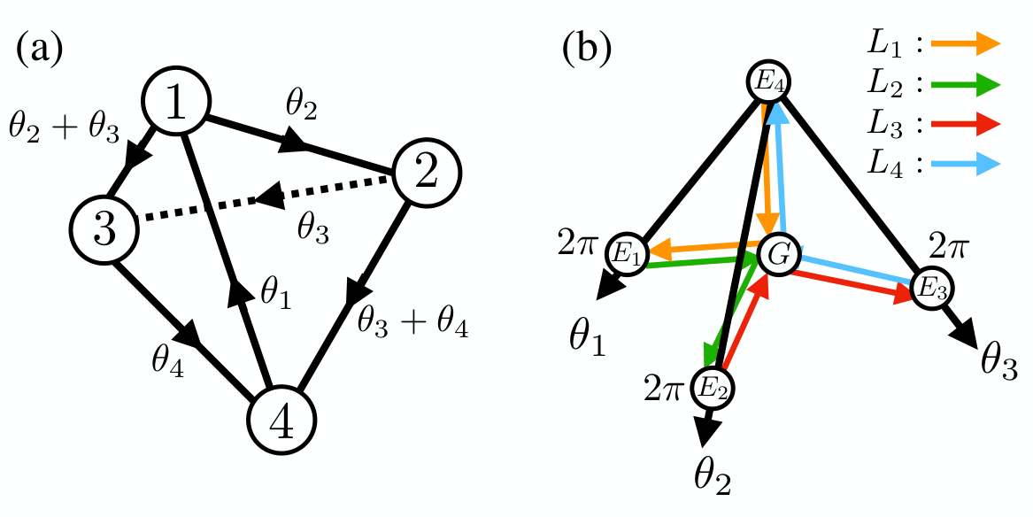
Due to the equivalence of the paths $L_{1},\cdots,L_{4}$, the spin-Berry phase is quantized into $\mathbb{Z}_{4}$ . Let us now derive it in detail. Tetrahedron is invariant for any exchange of the vertexes by the symmetric group $S_{4}$ Hatsugai_EPL2011SM. This implies that the original Hamiltonian $\mathcal{H}(\vec{\theta}=\vec{0})$ have $C_{3}$ symmetry and mirror symmetry with respect to the chosen downward tetrahedron, see Fig. S2. With finite $\vec{\theta}$, the symmetry is broken but instead we have

where $g$ is the $4\times 4$ unitary matrix satisfying $g\vec{\theta}=(\theta_{4},\theta_{1},\theta_{2},\theta_{3})$. Clearly, we have

where $i=1,\cdots,4$ and $\vec{f}_{5}\equiv\vec{f}_{1}$. This implies $\gamma_{1}\equiv\gamma_{2}\equiv\gamma_{3}\equiv\gamma_{4}\equiv\gamma\mod 2\pi$ as follows:

where $\vec{\theta}=g\vec{\theta}^{\prime}$, and we use $\partial/(\partial\theta_{l}^{\prime})|{G(g\vec{\theta}^{\prime})}\rangle=\left(U_{M}U_{C_{3}}\right)^{-1}\partial/(\partial\theta_{l}^{\prime})|{G(\vec{\theta}^{\prime})}\rangle$. Since the sum of the loop $L_{1},\cdots,L_{4}$ is equal to zero, implying

we have

where $n=0,1,2,3$.

Since the quantized value does not change unless the energy gap closes, $\gamma$ is an adiabatic invariant for gapped topological phases. For $U=0$, we have $\gamma=\pi$ for the HOTI while $\gamma=0$ for the band insulator. Let us now demonstrate it based on the decoupled limit. The HOTI phase includes the decoupled system with $t_{\bigtriangleup}=0$, whose Hamiltonian is given by $\mathcal{H}(\vec{\theta})=U_{-}(\vec{\theta})\mathcal{H}_{t}^{\bigtriangledown}U_{-}^{\dagger}(\vec{\theta})$. The spin-Berry connection $\vec{A}=(A_{1},\cdots,A_{4})$ is calculated as

where $|{G_{0}}\rangle=|{G(\vec{\theta}=\vec{0})}\rangle$. Because of symmetry, we have $\langle{G_{0}}|n_{1}^{-}|{G_{0}}\rangle=\cdots=\langle{G_{0}}|n_{4}^{-}|{G_{0}}\rangle\equiv s$ and

Consequently, the $\mathbb{Z}_{4}$ spin-Berry phase is given by

As mentioned in the main text, we have $s=-1/2$ in the half-filling, which implies $\gamma=\pi\mod 2\pi$. The other limit, i.e., $t_{\bigtriangledown}=0$ is included in the band insulating phase. Its Hamiltonian is given by $H(\vec{\theta})=H^{\bigtriangleup}$. Because of the independence of $\vec{\theta}$, we have $\gamma=0\mod 2\pi$.

In the scheme of the auxiliary field QMC, the Suzuki-Trotter decomposition Suzuki_1976SM; Trotter_1959SM is first applied to $e^{-\beta\mathcal{H}}$ as $e^{-\beta\mathcal{H}}\simeq\prod e^{-\Delta\tau\mathcal{H}_{t}/2}e^{-\Delta\tau\mathcal{H}_{U}}e^{-\Delta\tau\mathcal{H}_{t}/2}$, where $\mathcal{H}_{t}$ stands for the noninteracting parts in $\mathcal{H}$, and $\Delta\tau=\beta/M$ is a Trotter slice with $M$ being integer. The discrete Hubbard-Stratonovich transformation Hirsch_PRB1983SM is then applied to each term of $e^{-\Delta\tau Un_{i\uparrow}n_{i\downarrow}}$, introducing an auxiliary Ising-type variable at each spatial site in each imaginary time slice. The summation over the auxiliary fields involving the $MN_{\mathrm{s}}$ Ising variables is performed by Monte Carlo (MC) sampling.

We set the Trotter slice as $\Delta\tau=0.1$, for which the Trotter errors of order $O(\Delta\tau^{2})$ are sufficiently small compared with statistical errors of the MC sampling. As for the Hubbard-Stratonovich transformation, we employ one which couples to the spin degree of freedom. Typically, we perform $4\times 10^{3}$ MC sweeps for equilibration, followed by $8\times 10^{4}$ MC sweeps for measurement, which are divided into 20 bins to estimate the statistical error by the standard deviation. Each MC sweep consists of $MN_{\mathrm{s}}$ local updates and $N_{\mathrm{s}}$ global moves Scalettar_PRB1991SM. The simulations are carried out on the finite size clusters with $L$ up to 5 (8) corresponding to $N_{\mathrm{s}}=500$ (480) under the PBC (OBC).

The energy spectra as function of $\phi$ in the noninteracting limit are shown in Fig. S3. For the system under the PBC, the single-particle gap opens for the HOTI of $\phi<\phi_{\mathrm{c}1}^{0}\simeq 0.1$ and the BI of $\phi>\phi_{\mathrm{c}2}^{0}\simeq 0.4$. For the system under the OBC, the eightfold degenerate zero-energy states appear only in the HOTI. The averaged probability densities of these degenerated states are shown in Fig. S3(c) for $\phi=0.04$.

As shown in Fig. S4, we find $\phi_{\mathrm{c}1}^{U}=0.15(1)$ and $0.13(1)$ for $U=3$ and $1$. Above $\phi_{\mathrm{c}1}^{U}$, the strong finite-size effect is observed at low $T$ [see Figs. S4(c) and S4(f)], implying the absence of the bulk spin gap.

We confirm that the spin gap indeed vanishes at $\phi=\phi_{\mathrm{c}1}^{U}$ from magnetization plateaus under the magnetic field $h$ as shown in Fig. S5. It is noted that the simulations for $h\neq 0$ are possible without encountering the negative sign problem, since the model can be mapped onto the attractive model. The critical magnetic field, $h_{\mathrm{c}}$, is determined, in the similar way to $\phi_{\mathrm{c}1}^{U}$, as the point above which $\langle S_{\mathrm{tot}}^{z}\rangle/N_{\mathrm{UC}}$ deviates from $-1$. Since the spin gap is proportional to $h_{\mathrm{c}}$, the $\phi$-dependence of $h_{\mathrm{c}}$ in Fig. S5(c) represents how the spin gap decreases. Thus, the critical point $\phi_{\mathrm{c}1}^{U}$ is estimated as the point of $\phi$ for which $h_{\mathrm{c}}$ is zero. The result in Fig. S5(c) shows that $\phi_{\mathrm{c}1}^{U}$ estimated in this way turn out to agree well with those obtained from the $T$-dependence of $\langle S_{\mathrm{tot}}^{z}\rangle/N_{\mathrm{UC}}$ in Fig. S4 within the error bars.

References

- Hohenadler and Assaad (2013) M. Hohenadler and F. F. Assaad, J. Phys. Condens. Matter 25, 143201 (2013).
- Rachel (2018) S. Rachel, Reports Prog. Phys. 81, 116501 (2018).
- (3) Note that the topological Mott insulators studied here and in Ref. Raghu et al. 2008 are different, although the same term is used. In the former case, the topological Mott insulator is found as a Mott insulator possessing gapless edge spin-only excitations, while in the latter case band topology is induced from spontaneous symmetry breaking due to interactions.
- Pesin and Balents (2009) D. A. Pesin and L. Balents, Nat. Phys. 6, 376 (2009).
- Hasan and Kane (2010) M. Z. Hasan and C. L. Kane, Rev. Mod. Phys. 82, 3045 (2010).
- Moore (2010) J. E. Moore, Nature 464, 194 (2010).
- Qi and Zhang (2011) X.-L. Qi and S.-C. Zhang, Rev. Mod. Phys. 83, 1057 (2011).
- Hatsugai (1993a) Y. Hatsugai, Phys. Rev. Lett. 71, 3697 (1993a).
- Hatsugai (1993b) Y. Hatsugai, Phys. Rev. B 48, 11851 (1993b).
- Yamaji and Imada (2011) Y. Yamaji and M. Imada, Phys. Rev. B 83, 205122 (2011).
- Hohenadler et al. (2011) M. Hohenadler, T. C. Lang, and F. F. Assaad, Phys. Rev. Lett. 106, 100403 (2011).
- Yu et al. (2011) S.-L. Yu, X. C. Xie, and J.-X. Li, Phys. Rev. Lett. 107, 010401 (2011).
- Zheng et al. (2011) D. Zheng, G.-M. Zhang, and C. Wu, Phys. Rev. B 84, 205121 (2011).
- Yoshida et al. (2012) T. Yoshida, S. Fujimoto, and N. Kawakami, Phys. Rev. B 85, 125113 (2012).
- Tada et al. (2012) Y. Tada, R. Peters, M. Oshikawa, A. Koga, N. Kawakami, and S. Fujimoto, Phys. Rev. B 85, 165138 (2012).
- Yoshida et al. (2013) T. Yoshida, R. Peters, S. Fujimoto, and N. Kawakami, Phys. Rev. B 87, 085134 (2013).
- Yoshida et al. (2014) T. Yoshida, R. Peters, S. Fujimoto, and N. Kawakami, Phys. Rev. Lett. 112, 196404 (2014).
- Yoshida and Kawakami (2016) T. Yoshida and N. Kawakami, Phys. Rev. B 94, 085149 (2016).
- Bi et al. (2017) Z. Bi, R. Zhang, Y.-Z. You, A. Young, L. Balents, C.-X. Liu, and C. Xu, Phys. Rev. Lett. 118, 126801 (2017).
- Zhang et al. (2016) R. X. Zhang, C. Xu, and C. X. Liu, Phys. Rev. B 235128, 1 (2016).
- Benalcazar et al. (2017a) W. A. Benalcazar, B. A. Bernevig, and T. L. Hughes, Science 357, 61 (2017a).
- Schindler et al. (2018a) F. Schindler, A. M. Cook, M. G. Vergniory, Z. Wang, S. S. P. Parkin, B. A. Bernevig, and T. Neupert, Sci. Adv. 4, eaat0346 (2018a).
- Schindler et al. (2018b) F. Schindler, Z. Wang, M. G. Vergniory, A. M. Cook, A. Murani, S. Sengupta, A. Y. Kasumov, R. Deblock, S. Jeon, I. Drozdov, H. Bouchiat, S. Guéron, A. Yazdani, B. A. Bernevig, and T. Neupert, Nat. Phys. 14, 918 (2018b).
- Yue et al. (2019) C. Yue, Y. Xu, Z. Song, H. Weng, Y.-m. Lu, C. Fang, and X. Dai, Nat. Phys. 15, 577 (2019).
- Gray et al. (2019) M. J. Gray, J. Freudenstein, S. Y. F. Zhao, R. O’Connor, S. Jenkins, N. Kumar, M. Hoek, A. Kopec, S. Huh, T. Taniguchi, K. Watanabe, R. Zhong, C. Kim, G. D. Gu, and K. S. Burch, Nano Lett. 19, 4890 (2019).
- Liu et al. (2019a) B. Liu, G. Zhao, Z. Liu, and Z. F. Wang, Nano Lett. 19, 6492 (2019a).
- Sheng et al. (2019) X.-L. Sheng, C. Chen, H. Liu, Z. Chen, Z.-M. Yu, Y. X. Zhao, and S. A. Yang, Phys. Rev. Lett. 123, 256402 (2019).
- Chen et al. (2020) C. Chen, Z. Song, J.-Z. Zhao, Z. Chen, Z.-M. Yu, X.-L. Sheng, and S. A. Yang, Phys. Rev. Lett. 125, 056402 (2020).
- Hashimoto et al. (2017) K. Hashimoto, X. Wu, and T. Kimura, Phys. Rev. B 95, 165443 (2017).
- Benalcazar et al. (2017b) W. A. Benalcazar, B. A. Bernevig, and T. L. Hughes, Phys. Rev. B 96, 245115 (2017b).
- Song et al. (2017) Z. Song, Z. Fang, and C. Fang, Phys. Rev. Lett. 119, 246402 (2017).
- Fukui and Hatsugai (2018) T. Fukui and Y. Hatsugai, Phys. Rev. B 98, 035147 (2018).
- Ezawa (2018a) M. Ezawa, Phys. Rev. Lett. 120, 026801 (2018a).
- Ezawa (2018b) M. Ezawa, Phys. Rev. B 98, 045125 (2018b).
- Langbehn et al. (2017) J. Langbehn, Y. Peng, L. Trifunovic, F. von Oppen, and P. W. Brouwer, Phys. Rev. Lett. 119, 246401 (2017).
- Ezawa (2018c) M. Ezawa, Phys. Rev. Lett. 121, 116801 (2018c).
- Ezawa (2018d) M. Ezawa, Phys. Rev. B 97, 155305 (2018d).
- Khalaf (2018) E. Khalaf, Phys. Rev. B 97, 205136 (2018).
- Liu et al. (2019b) T. Liu, Y.-R. Zhang, Q. Ai, Z. Gong, K. Kawabata, M. Ueda, and F. Nori, Phys. Rev. Lett. 122, 076801 (2019b).
- Călugăru et al. (2019) D. Călugăru, V. Juričić, and B. Roy, Phys. Rev. B 99, 041301 (2019).
- Araki et al. (2019) H. Araki, T. Mizoguchi, and Y. Hatsugai, Phys. Rev. B 99, 085406 (2019).
- Araki et al. (2020) H. Araki, T. Mizoguchi, and Y. Hatsugai, Phys. Rev. Res. 2, 012009 (2020).
- Mizoguchi et al. (2019) T. Mizoguchi, H. Araki, and Y. Hatsugai, J. Phys. Soc. Jpn. 88, 104703 (2019).
- You et al. (2018) Y. You, T. Devakul, F. J. Burnell, and T. Neupert, Phys. Rev. B 98, 235102 (2018).
- Kudo et al. (2019) K. Kudo, T. Yoshida, and Y. Hatsugai, Phys. Rev. Lett. 123, 196402 (2019).
- Dubinkin and Hughes (2019) O. Dubinkin and T. L. Hughes, Phys. Rev. B 99, 235132 (2019).
- Bibo et al. (2020) J. Bibo, I. Lovas, Y. You, F. Grusdt, and F. Pollmann, Phys. Rev. B 102, 041126 (2020).
- Peng et al. (2019) C. Peng, R.-Q. He, and Z.-Y. Lu, Phys. Rev. B 102, 045110 (2019).
- (49) J. Guo, J. Sun, X. Zhu, C.-A. Li, H. Guo, and S. Feng, Quantum Monte Carlo study of higher-order topological spin phases, arXiv:2010.05402 .
- Imhof et al. (2018) S. Imhof, C. Berger, F. Bayer, J. Brehm, L. W. Molenkamp, T. Kiessling, F. Schindler, C. H. Lee, M. Greiter, T. Neupert, and R. Thomale, Nat. Phys. 14, 925 (2018).
- Peterson et al. (2018) C. W. Peterson, W. A. Benalcazar, T. L. Hughes, and G. Bahl, Nature 555, 346 (2018).
- Serra-Garcia et al. (2018) M. Serra-Garcia, V. Peri, R. Süsstrunk, O. R. Bilal, T. Larsen, L. G. Villanueva, and S. D. Huber, Nature 555, 342 (2018).
- Ni et al. (2019) X. Ni, M. Weiner, A. Alù, and A. B. Khanikaev, Nat. Mater. 18, 113 (2019).
- Xue et al. (2019a) H. Xue, Y. Yang, F. Gao, Y. Chong, and B. Zhang, Nat. Mater. 18, 108 (2019a).
- Xue et al. (2019b) H. Xue, Y. Yang, G. Liu, F. Gao, Y. Chong, and B. Zhang, Phys. Rev. Lett. 122, 244301 (2019b).
- Kempkes et al. (2019) S. N. Kempkes, M. R. Slot, J. J. van den Broeke, P. Capiod, W. A. Benalcazar, D. Vanmaekelbergh, D. Bercioux, I. Swart, C. Morais Smith, J. J. van den Broeke, P. Capiod, W. A. Benalcazar, D. Vanmaekelbergh, D. Bercioux, I. Swart, and C. M. Smith, Nat. Mater. 18, 1292 (2019).
- Weiner et al. (2020) M. Weiner, X. Ni, M. Li, A. Alù, and A. B. Khanikaev, Sci. Adv. 6, eaay4166 (2020).
- Hatsugai and Maruyama (2011) Y. Hatsugai and I. Maruyama, Euro. Phys. Lett. 95, 20003 (2011).
- Blankenbecler et al. (1981) R. Blankenbecler, D. J. Scalapino, and R. L. Sugar, Phys. Rev. D 24, 2278 (1981).
- Hirsch (1985) J. E. Hirsch, Phys. Rev. B 31, 4403 (1985).
- White et al. (1989) S. R. White, D. J. Scalapino, R. L. Sugar, E. Y. Loh, J. E. Gubernatis, and R. T. Scalettar, Phys. Rev. B 40, 506 (1989).
- Scalettar et al. (1991) R. Scalettar, R. Noack, and R. Singh, Phys. Rev. B 44, 10502 (1991).
- Assaad and Evertz (2008) F. Assaad and H. Evertz, in Comput. Many-Particle Phys., edited by F. H., S. R., and W. A. (Springer Berlin Heidelberg, Berlin, Heidelberg, 2008) pp. 277–356.
- Loh et al. (1990) E. Y. Loh, J. E. Gubernatis, R. T. Scalettar, S. R. White, D. J. Scalapino, and R. L. Sugar, Phys. Rev. B 41, 9301 (1990).
- dos Santos (1993) R. R. dos Santos, Phys. Rev. B 48, 3976 (1993).
- (66) See Supplemental Material for details of the spin-Berry phase, the numerical details, and additional results.
- Otsuka et al. (2002) Y. Otsuka, Y. Morita, and Y. Hatsugai, Phys. Rev. B 66, 073109 (2002).
- Otsuka and Hatsugai (2003) Y. Otsuka and Y. Hatsugai, Phys. B Condens. Matter 329-333, 580 (2003).
- Morita et al. (2004) Y. Morita, Y. Hatsugai, and Y. Otsuka, Phys. Rev. B 70, 245101 (2004).
- (70) The superconducting phase in terms of the attractive model corresponds to a ferromagnetic state in the plane, which should emerge somewhere in the MI region of the phase diagram.
- Ortiz et al. (2019) B. R. Ortiz, L. C. Gomes, J. R. Morey, M. Winiarski, M. Bordelon, J. S. Mangum, I. W. H. Oswald, J. A. Rodriguez-Rivera, J. R. Neilson, S. D. Wilson, E. Ertekin, T. M. McQueen, and E. S. Toberer, Phys. Rev. Mater. 3, 094407 (2019).
- Ortiz et al. (2021) B. R. Ortiz, P. M. Sarte, E. Kenney, S. M. L. Teicher, R. Seshadri, M. J. Graf, and S. D. Wilson, Phys. Rev. Mater. 5, 034801 (2021).
- Jiang et al. (2021) Y.-X. Jiang, J.-X. Yin, M. M. Denner, N. Shumiya, B. R. Ortiz, G. Xu, Z. Guguchia, J. He, M. S. Hossain, X. Liu, J. Ruff, L. Kautzsch, S. S. Zhang, G. Chang, I. Belopolski, Q. Zhang, T. A. Cochran, D. Multer, M. Litskevich, Z.-J. Cheng, X. P. Yang, Z. Wang, R. Thomale, T. Neupert, S. D. Wilson, and M. Z. Hasan, Nat. Mater. 20, 1353 (2021).
- Liang et al. (2021) Z. Liang, X. Hou, F. Zhang, W. Ma, P. Wu, Z. Zhang, F. Yu, J.-J. Ying, K. Jiang, L. Shan, Z. Wang, and X.-H. Chen, Phys. Rev. X 11, 031026 (2021).
- Raghu et al. (2008) S. Raghu, X.-L. Qi, C. Honerkamp, and S.-C. Zhang, Phys. Rev. Lett. 100, 156401 (2008).
Supplemental Material:
- (1) Y. Hatsugai and I. Maruyama, Euro. Phys. Lett 95, 200003 (2011).
- (2) K. Kudo, Ph. D. thesis (University of Tsukuba, 2021).
- (3) H. Araki, private communication.
- (4) M. Suzuki, Commun. Math. Phys. 51, 183 (1976).
- (5) H. F. Trotter, Proc. Am. Math. Soc. 10, 545 (1959).
- (6) J. E. Hirsch, Phys. Rev. B 28, 4059 (1983).
- (7) R. Scalettar, R. Noack, and R. Singh, Phys. Rev. B 44, 10502 (1991).