Vibration Analysis of Piezoelectric Kirchhoff-Love Shells based on Catmull-Clark Subdivision Surfaces

Zhaowei Liu zhaowei.liu@glasgow.ac.uk Address: Glasgow Computational Engineering Centre, University of Glasgow, Glasgow, G12 8LT, United Kingdom Andrew McBride Prashant Saxena Luca Heltai Address: SISSA (International School for Advanced Studies), Via Bonomea 265, 34136 Trieste, Italy Yilin Qu Address: State Key Laboratory for Strength and Vibration of Mechanical Structures, Xi’an Jiaotong University, Xi’an 710049, Shaanxi, China Paul Steinmann Address: Institute of Applied Mechanics, Friedrich-Alexander Universität Erlangen-Nürnberg, D-91052, Erlangen, Germany

Abstract

An isogeometric Galerkin approach for analysing the free vibrations of piezoelectric shells is presented. The shell kinematics is specialised to infinitesimal deformations and follow the Kirchhoff-Love hypothesis. Both the geometry and physical fields are discretised using Catmull-Clark subdivision bases. It provides the required $C^{1}$ continuous discretisation for the Kirchhoff-Love theory. The crystalline structure of piezoelectric materials is described using an anisotropic constitutive relation. Hamilton’s variational principle is applied to the dynamic analysis to derive the weak form of the governing equations. The coupled eigenvalue problem is formulated by considering the problem of harmonic vibration in the absence of external load. The formulation for the purely elastic case is verified using a spherical thin shell benchmark. Thereafter, the piezoelectric effect and vibration modes of a transverse isotropic curved plate are analysed and evaluated for the Scordelis-Lo roof problem. Finally, the eigenvalue analysis of a CAD model of a piezoelectric speaker shell structure showcases the ability of the proposed method to handle complex geometries.

keywords

piezoelectricity ,Kirchhoff-Love shell ,isogeometric analysis ,Catmull-Clark subdivision surfaces ,Eigienvalue analysis

^†^†corresponding: Corresponding author

1 Introduction

Piezoelectricity is a reversible two-way coupling effect resulting from electromechanical interactions in certain crystalline materials. In 1880, Curie and Curie 1880 discovered the direct piezoelectric effect whereby a mechanical excitation generates an electrical potential. Shortly thereafter, Lippmann 1881 derived the converse piezoelectric effect from fundamental thermodynamic principles. In 1881, Curie and Curie 1881 proved its existence as a strain that occurs when an electric field is applied. Shortly after the piezoelectric phenomenon was discovered, Langevin and Rutherford independently applied the piezoelectric effect for submarine detection devices [38]. In the subsequent hundred years, the piezoelectric effect has been extensively studied and a wide range of novel piezoelectric materials and devices invented and applied to engineering applications. The direct piezoelectric effect is used in sensors/transducers [54, 35, 1, 62, 48, 56] and energy harvesters [28, 40], while the converse piezoelectric effect is used in resonators [9, 50, 32] and actuators [30, 26, 34].

Piezoelectric sensors and actuators are often constructed from films, plates and shells as they can generate large strains under small loads. Early studies of piezoelectric structures focused on simple geometries such as rods [53], plates [61, 60] and cylindrical shells [49, 51]. Laminated piezoelectric plates [31, 23] are also well studied. With the development of active, adaptive and smart structures, piezoelectric materials are widely used because of their ability to achieve a precise and complex mechanical response to electrical loads. This motivates the requirement for analysis of piezoelectric structures with complex geometries. The finite element method is the ideal modelling framework to analyse such complex structures and to deal with inherent nonlinearities. Allik and Hughes 1970 proposed a three-dimensional finite element method for electroelastic analyses, focussing mainly on piezoelectric vibrations. The early works of the piezoelectric finite element method have been reviewed by Benjeddou 2000. Tzou and Tseng 1990 evaluated the performance of intelligent piezoelectric thin plates using a finite element approach. Hwang and Park 1993 developed a finite element model of laminated plates with piezoelectric sensors and actuators. A nonlinear finite element approach to phase transition in piezoelectric materials was proposed by Ghandi and Hagood 1996, while Lam et al. 1997 analysed piezoelectric composite laminates. A static and dynamic analysis of a piezoelectric bimorph was undertaken by Wang 2004.

Although many three-dimensional finite element approaches for piezoelectric structures have been proposed, work on piezoelectric Kirchhoff-Love shells is limited. Kirchhoff-Love and Reissner-Mindlin shell theories categorise shells into ”thin” and ”thick” according to the ratio of curvature radius to thickness. The Kirchhoff-Love shell theory, also called ”classical shell model”, is tailored to thin shells. The Reissner-Mindlin shell theory is an extension of the Kirchhoff-Love theory, which can be applied to both thin and thick shells since it accounts for shear deformations. However, Reissner-Mindlin shells theory require additional rotational degrees of freedom, resulting in a larger system matrix than the Kirchhoff-Love shell theory. Kirchhoff-Love shells require only three translational degrees of freedom, which is computationally more efficient. However, the Kirchhoff-Love finite element method requires $C^{1}$ continuity of the basis functions while a conventional Lagrangian interpolation only provides $C^{0}$ continuity.

Hughes et al. 2005 presented the framework for isogeometric analysis (IGA) in 2005. IGA provides higher-order continuity by using splines as interpolation functions and it allows for exact geometric representation which completely eliminates geometry error in the numerical solution. However, volume parameterisation of a Computer Aided Desgin (CAD) model is the most challenging problem for IGA [20]. Shell formulations are well suited for IGA since they only require a discretisation of the mid-surfaces of the shell. Kiendl et al. 2009 developed an isogeometric approach for Kirchhoff-Love shells using Non-Uniform Rational B-Splines (NURBS). Isogeometric Reissner-Mindlin shell has also been well studied in [11, 12]. Cirak et al. 2000 developed a $C^{1}$ conforming discretisation based on Loop subdivision surfaces for an elastic Kirchhoff-Love shell formulation and applied it to hyperelastic thin shells [17]. Subdivision surfaces is an alternative to NURBS surfaces and is a mature geometry modelling method widely used in the animation and gaming industry. An attractive feature of subdivision surfaces is that they can be evaluated using spline functions, while retaining a simple polygonal mesh data structure able to represent complex geometries. Extraordinary vertices in the mesh allow for local refinement and patch conforming, both challenges faced by NURBS. Subdivision surfaces shell formulations have been extended to applications including shell fracture [18], shape optimisation [6, 14], fluid-structure interaction [15], non-manifold geometry [16] and structural-acoustic analysis [44]. The ability of subdivision surfaces to analyse thin shells underpins the analysis of the electromechanical coupled thin shells presented here.

Applications for piezoelectric shells, such as resonators, actuators and energy harvesters, often involve the structural dynamics. Thus, understanding the effect of electroelastic coupling on the vibration mode of piezoelectric structures is critical. The coupling effect will influence the lattice structure of the piezoelectric material and enhance the stiffness of such structure via the so-called ”piezoelectric stiffening” effect [36]. Thus, the natural frequencies of vibration modes increase. This effect is used in laminated beams [64] and plates [25] with piezoelectric actuators to enhance their stiffness. However, the ”piezoelectric stiffening” effect of piezoelectric thin shells with complex geometry is seldom studied. This work provides a numerical analysis tool for understanding these effects in piezoelectric thin shells.

The proposed method adopts Catmull-Clark subdivision surfaces to formulate a novel isogeometric Galerkin approach to analyse piezoelectric thin shells with arbitrary geometries. The formulation for analysing the thin shell considers three different electric conditions, which are no electrodes, prescribed voltage with electrodes and short-circuited electrode. These are comprehensively derived and summarised. A method to tailor the natural frequency of piezoelectric curved plate by changing its curvature is also presented. In addition, the ”piezoelectric stiffening” effect of piezoelectric thin shells with complex geometry is also examined.

This contribution is organised as follows. Section 2 introduces the notation and defines various coordinate systems used throughout the manuscript. Section 3 illustrates the kinematics of Kirchhoff-Love shells. Section 4 briefly reiterates the theory of Catmull-Clark subdivision surfaces. Energy considerations required for piezoelectric thin shells are presented in Section 5.1 and 5.2. Hamilton’s variational principle is applied and the resulting weak form of the governing equations of piezoelectric shells derived in Section 5.6. Section 5.7 discretises the weak form of the governing equations using Catmull-Clark subdivision bases resulting in the discrete system of equations. Finally, Section 6 presents three numerical examples to demonstrate the ability of the proposed piezoelectric thin shell method to deal with various geometries and a range of mechanical and coupled problems.

2 Notations

Brackets:

Two types of brackets are used. Square brackets $[]$ are used to clarify the order of operations in an algebraic expression. Circular brackets $()$ are used to denote the parameters of a function. If brackets are used to denote an interval then $()$ stands for an open interval and $[]$ is a closed interval.

Symbols:

A variable typeset in a normal weight font represents a scalar. A bold weight font denotes a first or second-order tensor. An overline indicates that the variable is defined with respect to the reference configuration and if absent, the variable is defined with respect to the current (deformed) configuration. A scalar variable with superscript or subscript indices normally represents the components of a vector or second-order tensor. Upright font is used to denote matrices and vectors.

Indices $i,j,k,\dots$ vary from $1$ to $3$ while $a,b,c,\dots$ , used as surface variable components, vary from $1$ to $2$ . Einstein summation convention is used throughout.

The comma symbol in a subscript represents partial derivative, for example, $A_{,b}$ is the partial derivative of $A$ with respect to its $b^{\text{th}}$ component. $\nabla(\bullet)$ is the three-dimensional gradient operator.

Coordinates:

$\mathbf{c}_{i}$ represent the basis vectors of an orthonormal system in three-dimensional Euclidean space and $x,y$ and $z$ are its components. $\boldsymbol{\xi}_{i}$ denote the orthonormal basis vectors in the local element space and $\xi,\eta$ and $\zeta$ are its coordinate components. The three covariant basis vectors for a surface point are denoted as $\mathbf{a}_{i}$ , where $\mathbf{a}_{1},\mathbf{a}_{2}$ are two tangential vectors and $\mathbf{a}_{3}$ is the normal vector.

3 Kirchhoff-Love shell kinematics

The Kirchhoff-Love hypothesis can be applied to three-dimensional structures in which one dimension is much smaller than the other two. Important examples include plates and shells. It is assumed that lines perpendicular to the mid-surface remain straight and perpendicular to the mid-surface after deformation (see Figure 1).

Figure 1: Kirchhoff-Love shell coordinates

The shell occupies the physical domain $\Omega$ and has a uniform thickness $h$ . The thickness does not change upon deformation. The mid-surface of the shell is denoted by $\Gamma$ .

Refer to caption — Figure 2: Reference and deformed configurations for the mid-surface of a Kirchhoff-Love shell.

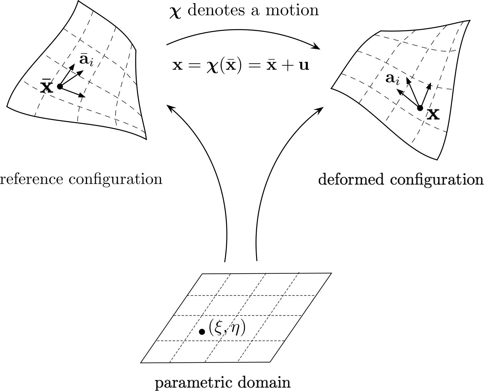
Figure 2 shows the reference and deformed configurations of the mid-surface. Points on the mid-surface in the reference and the deformed configurations are denoted by $\bar{\mathbf{x}}$ and $\mathbf{x}$ . respectively, and are obtained as map from the parametric coordinates $\xi$ and $\eta$ . The position vector of a point in the deformed configuration $\mathbf{r}$ is computed using the mid-surface point $\mathbf{x}$ and the normal vector $\mathbf{n}$ as

\mathbf{r}(\xi,\eta,\zeta)=\mathbf{x}(\xi,\eta)+\zeta\mathbf{n}(\xi,\eta),

(1)

where $\zeta\in[-{h}/{2},{h}/{2}]$ . A mid-surface point in the deformed configuration ${\mathbf{x}}$ can be expressed as

\mathbf{x}=\bar{\mathbf{x}}+\mathbf{u},

(2)

where $\mathbf{u}$ denotes the displacement.

3.1 Green-Lagrangian strain tensor

The covariant basis vectors of the tangent plane of the mid-surface in the reference and the deformed configurations are defined by

\bar{\mathbf{a}}_{1}=\frac{\partial\bar{\mathbf{x}}}{\partial\xi},\quad\bar{\mathbf{a}}_{2}=\frac{\partial\bar{\mathbf{x}}}{\partial\eta},\quad\text{and}\quad{\mathbf{a}}_{1}=\frac{\partial{\mathbf{x}}}{\partial\xi},\quad{\mathbf{a}}_{2}=\frac{\partial{\mathbf{x}}}{\partial\eta}.

(3)

Thus, the normal vectors in the two configurations can be computed as

\bar{\mathbf{n}}=\bar{\mathbf{a}}_{3}=\frac{\bar{\mathbf{a}}_{1}\times\bar{\mathbf{a}}_{2}}{\bar{J}},\quad\text{and}\quad{\mathbf{n}}={\mathbf{a}}_{3}=\frac{{\mathbf{a}}_{1}\times{\mathbf{a}}_{2}}{{J}},

(4)

where $\bar{J}$ and $J$ are the respective Jacobians given by

\bar{J}=|\bar{\mathbf{a}}_{1}\times\bar{\mathbf{a}}_{2}|,\quad\text{and}\quad J=|{\mathbf{a}}_{1}\times{\mathbf{a}}_{2}|.

(5)

Thus, the covariant components of the metric tensor for the mid-surface points $\bar{\mathbf{x}}$ and $\mathbf{x}$ are respectively given by

\bar{a}_{ij}=\bar{\mathbf{a}}_{i}\cdot\bar{\mathbf{a}}_{j},\quad\text{and}\quad{a}_{ij}={\mathbf{a}}_{i}\cdot{\mathbf{a}}_{j}.

(6)

The contravariant metric tensors are defined by

\bar{a}^{ik}\bar{a}_{kj}=\delta^{i}_{j},\quad\text{and}\quad a^{ik}a_{kj}=\delta^{i}_{j},

(7)

where $\delta^{i}_{j}$ denotes the Kronecker Delta. The three-dimensional covariant basis vectors for the shell in the reference and the deformed configurations are respectively given by

\bar{\mathbf{g}}_{1}=\frac{\partial\bar{\mathbf{r}}}{\partial\xi}=\bar{\mathbf{a}}_{1}+\zeta\bar{\mathbf{a}}_{3,1},\quad\bar{\mathbf{g}}_{2}=\frac{\partial\bar{\mathbf{r}}}{\partial\eta}=\bar{\mathbf{a}}_{2}+\zeta\bar{\mathbf{a}}_{3,2},\quad\bar{\mathbf{g}}_{3}=\frac{\partial\bar{\mathbf{r}}}{\partial\zeta}=\bar{\mathbf{a}}_{3},

(8)

and

{\mathbf{g}}_{1}=\frac{\partial{\mathbf{r}}}{\partial\xi}={\mathbf{a}}_{1}+\zeta{\mathbf{a}}_{3,1},\quad{\mathbf{g}}_{2}=\frac{\partial{\mathbf{r}}}{\partial\eta}={\mathbf{a}}_{2}+\zeta{\mathbf{a}}_{3,2},\quad{\mathbf{g}}_{3}=\frac{\partial{\mathbf{r}}}{\partial\zeta}={\mathbf{a}}_{3},

(9)

where $(\bullet)_{,1}$ and $(\bullet)_{,2}$ represent the partial differentials with respect to $\xi$ and $\eta$ , respectively. The components of the covariant metric tensors are defined by

\bar{g}_{ij}=\bar{\mathbf{g}}_{i}\cdot\bar{\mathbf{g}}_{j}\quad\text{and}\quad g_{ij}=\mathbf{g}_{i}\cdot\mathbf{g}_{j},

(10)

which allows one to define the Green-Lagrange strain tensor $\mathbf{S}_{n}$ as

\mathbf{S}_{n}\coloneqq\frac{1}{2}[g_{ij}-\bar{g}_{ij}]\bar{\mathbf{g}}^{i}\otimes\bar{\mathbf{g}}^{j},

(11)

where $\bar{\mathbf{g}}^{i}$ denote the contravariant basis vectors defined by

\bar{\mathbf{g}}^{i}\cdot\bar{\mathbf{g}}_{j}=\delta^{i}_{j}.

(12)

3.2 Linearisation and simplification of the strain tensor

On substituting equations (8) and (9) into (11) and ignoring higher-order terms, the Green-Lagrange strain tensor linearised in $\zeta$ follows as

\mathbf{S}=\mathbf{A}+\zeta\mathbf{B}.

(13)

The components of the tensors $\mathbf{A}$ and $\mathbf{B}$ are $\alpha_{ij}$ and $\beta_{ij}$ , respectively, with $\alpha_{13}$ and $\alpha_{23}$ measuring the shearing in the normal direction $\bar{\mathbf{a}}_{3}$ , and are zero under the Kirchhoff-Love assumption. The stretching in normal direction is given by $\alpha_{33}=0$ and it vanishes due to the assumption that the thickness does not change with deformation. Similarly, $\beta_{i3}=0$ as the normal vector is perpendicular to the two basis vectors. Thus, the two tensors $\mathbf{A}$ and $\mathbf{B}$ reduce to two-dimensional tensors in the subspace defined with two contravariant basis vectors as

\mathbf{A}\coloneqq\alpha_{ab}\,\mathbf{\bar{g}}^{a}\otimes\mathbf{\bar{g}}^{b}\quad\text{and}\quad\mathbf{B}\coloneqq\beta_{ab}\,\mathbf{\bar{g}}^{a}\otimes\mathbf{\bar{g}}^{b},

(14)

where their components are computed as

\displaystyle{\alpha}_{ab}=\frac{1}{2}[\mathbf{a}_{a}\cdot\mathbf{a}_{b}-\bar{\mathbf{a}}_{a}\cdot\bar{\mathbf{a}}_{b}]\quad\text{and}\quad{\beta}_{ab}=\mathbf{a}_{a}\cdot\mathbf{a}_{3,b}-\bar{\mathbf{a}}_{a}\cdot\bar{\mathbf{a}}_{3,b}.

(15)

The membrane strain components are denoted as $\alpha_{ab}$ while the bending strain components $\beta_{ab}$ measure the change in the curvature of the shell. In order to compute the bending strain tensor, the product rule of differentiation is applied and the components expressed as

\beta_{ab}=\bar{\mathbf{a}}_{a,b}\cdot\bar{\mathbf{a}}_{3}-{\mathbf{a}}_{a,b}\cdot{\mathbf{a}}_{3}.

(16)

On substituting Equation (2) into the membrane and bending strains, the components can eventually be computed to first order in $\mathbf{u}$ as

	$\displaystyle\alpha_{ab}=$	$\displaystyle\frac{1}{2}[\bar{\mathbf{a}}_{a}\cdot\mathbf{u}_{,b}+{\mathbf{u}}_{,a}\cdot\bar{\mathbf{a}}_{b}],$		(17)
	$\displaystyle\beta_{ab}=$	$\displaystyle-\mathbf{u}_{,{ab}}\cdot\bar{\mathbf{a}}_{3}+\frac{1}{\bar{J}}\big[\mathbf{u}_{,1}\cdot[\bar{\mathbf{a}}_{a,b}\times\bar{\mathbf{a}}_{2}]+\mathbf{u}_{,2}\cdot[\bar{\mathbf{a}}_{1}\times\bar{\mathbf{a}}_{a,b}]\big]+\frac{\bar{\mathbf{a}}_{3}\cdot\bar{\mathbf{a}}_{a,b}}{\bar{J}}\big[\mathbf{u}_{,1}\cdot[\bar{\mathbf{a}}_{2}\times\bar{\mathbf{a}}_{3}]+\mathbf{u}_{,2}\cdot[\bar{\mathbf{a}}_{3}\times\bar{\mathbf{a}}_{1}]\big].$		(18)

Thus, the linearised strain tensor $\mathbf{S}$ is computed using the covariant basis vectors along with the first and second derivatives of the displacement $\mathbf{u}$ .

4 Catmull-Clark subdivision surfaces

Kirchhoff-Love shells require that the test and trial functions of the Galerkin method are in the Hilbert space $H^{2}(\Omega)$ [19]. Hence a $C^{1}$ continuous discretisation is required. Conventional Lagrangian bases only provide $C^{0}$ continuity. Catmull–Clark subdivision surfaces [57], which adopt cubic B-splines as interpolating functions, display $C^{2}$ continuity everywhere except at the surface points related to extraordinary vertices [52], where continuity is only $C^{1}$ . Figure 3 shows an example of cubic B-splines for one dimensional elements. The Catmull-Clark subdivision surfaces adopt a tensor-product structure of two cubic B-splines to interpolate points on a two-dimensional surface. Figure 4 shows a smooth surface constructed by successive subdivision from a coarse polygonal mesh using the Catmull-Clark subdivision scheme [13].

The surface, composed of points $\bar{\mathbf{x}}\in\Gamma$ , can be interpolated using the basis functions (cubic B-splines) and control points as

\bar{\mathbf{x}}=\sum_{A=0}^{n_{b}-1}N^{A}\mathbf{P}_{A},

(19)

where $n_{b}$ is the number of basis functions. The $A^{\text{th}}$ basis function is denoted as $N^{A}$ and $\mathbf{P}_{A}$ denotes the $A^{\text{th}}$ control point. An element of a regular patch with $16$ basis functions is shown in Figure 4. We note that the control points are not necessarily on the surface $\Gamma$ . Further details of an isogeometric Galerkin method using Catmull-Clark subdivision surfaces can be found in [45].

5 Piezoelectric shell formulation

5.1 Energy densities

The electric enthalpy density per unit volume for a coupled piezoelectric problem [47, 58] is most generally defined by

\displaystyle\mathcal{H}(\mathbf{S},\mathbf{E})=W_{\text{ela}}(\mathbf{S})-W_{\text{piezo}}(\mathbf{S},\mathbf{E})-W_{\text{elec}}(\mathbf{E}).

(20)

The electric enthalpy density contains the elastic energy density $W_{\text{ela}}$ , the piezoelectric energy density $W_{\text{piezo}}$ and the electric energy density $W_{\text{elec}}$ . The electric field is denoted as $\mathbf{E}$ . The piezoelectric and electric energy densities are expressed as

W_{\text{piezo}}(\mathbf{S},\mathbf{E})=\mathbf{E}\cdot[\mathbf{e}:\mathbf{S}]=e^{ijk}E_{i}[\alpha_{jk}+\zeta\beta_{jk}],

(21)

and

W_{\text{elec}}(\mathbf{E})=\frac{1}{2}[\boldsymbol{\kappa}\cdot\mathbf{E}]\cdot\mathbf{E}=\frac{1}{2}\kappa^{ij}E_{i}E_{j},

(22)

respectively. The components of the third-order piezoelectric tensor $\mathbf{e}$ are $e^{ijk}$ while $\kappa^{ij}$ are the components of the second-order dielectric tensor $\boldsymbol{\kappa}$ . Since the structure is thin and has uniform thickness, we introduce the quadratic elastic strain energy density per unit area $\widetilde{W}_{\text{ela}}$ for the Kirchhoff-Love shell as

\widetilde{W}_{\text{ela}}(\mathbf{S})=\int_{-\frac{h}{2}}^{\frac{h}{2}}W_{\text{ela}}(\mathbf{S})\,\mathrm{d}\zeta.

(23)

The piezoelectric material is normally anisotropic due to the interaction between the mechanical and electrical states in crystalline materials with no inversion symmetry. Thus, with $\mathbf{S}=\mathbf{A}+\zeta\mathbf{B}$ , one defines a general formulation for the elastic energy density per unit area by

\widetilde{W}_{\text{ela}}(\mathbf{S})=\widetilde{W}_{\text{ela}}(\mathbf{A},\mathbf{B})=\frac{h}{2}\left[[\mathbf{A}:\mathbf{C}:\mathbf{A}]+\frac{h^{2}}{12}[\mathbf{B}:\mathbf{C}:\mathbf{B}]\right],

(24)

where $\mathbf{C}$ is the fourth-order elastic tensor which can be defined using the covariant base vectors by

\mathbf{C}={C}^{ijkl}\bar{\mathbf{g}}_{i}\otimes\bar{\mathbf{g}}_{j}\otimes\bar{\mathbf{g}}_{k}\otimes\bar{\mathbf{g}}_{l}=\tilde{C}^{mnop}{\mathbf{t}}_{m}\otimes{\mathbf{t}}_{n}\otimes{\mathbf{t}}_{o}\otimes{\mathbf{t}}_{p}.

(25)

The preferable anisotropy directions of the piezoelectric material is denoted as $\mathbf{t}_{m}$ . Therefore, the components of the elasticity tensor are related by

{C}^{ijkl}=\tilde{C}^{mnop}[\bar{\mathbf{g}}^{i}\cdot\mathbf{t}_{m}][\bar{\mathbf{g}}^{j}\cdot\mathbf{t}_{n}][\bar{\mathbf{g}}^{k}\cdot\mathbf{t}_{o}][\bar{\mathbf{g}}^{l}\cdot\mathbf{t}_{p}].

(26)

5.2 Kinetic energy

The kinetic energy of a Kirchhoff-Love thin shell is defined by

\Pi_{\text{kin}}=\frac{\rho h}{2}\int_{\Gamma}\left[\frac{\partial u_{i}}{\partial t}\right]^{2}\,\mathrm{d}\Gamma

(27)

where $\rho$ denotes the mass density per unit volume which is here assumed constant.

5.3 Electric enthalpy

The total electric enthalpy of the system is composed of three parts:

\displaystyle\mathfrak{E}(\mathbf{S},\mathbf{E})=\Pi_{\text{ela}}(\mathbf{S})-\Pi_{\text{piezo}}(\mathbf{S},\mathbf{E})-\Pi_{\text{elec}}(\mathbf{E}),

(28)

where $\Pi_{\text{piezo}}$ is the piezoelectric energy. The dielectric energy is denoted as $\Pi_{\text{elec}}$ and the elastic energy is defined by

\Pi_{\text{ela}}(\mathbf{S})=\int_{\Gamma}\widetilde{W}_{\text{ela}}(\mathbf{S})\,\mathrm{d}\Gamma.

(29)

To consider the piezoelectric and the dielectric energy for a thin shell formulation, a power series expansion is applied to the electric potential with respect to the thickness coordinate $\zeta$ [59] and the first three terms are retained, that is

\phi(\mathbf{r}(\xi,\eta,\zeta))\approx\phi^{(0)}(\mathbf{x}(\xi,\eta))+\zeta\phi^{(1)}(\mathbf{x}(\xi,\eta))+\left[\zeta^{2}-\left[\frac{h}{2}\right]^{2}\right]\phi^{(2)}(\mathbf{x}(\xi,\eta)).

(30)

The electric field is computed as

\mathbf{E}=-\nabla\phi,

(31)

and it can be expressed using contravariant basis vector as

\mathbf{E}=E_{i}\bar{\mathbf{g}}^{i},

(32)

Due to the large relative permittivity of piezoelectric materials, the electric field in the surrounding free space is neglected. The energy contributions and hence the coupling effect depends on the configuration of the piezoelectric shell structure. Unelectroded and electroded shells along with a special short-circuited case, as displayed in Figure 5 are three options considered here.

$\bullet$ Shell with no electrodes

In this case, the shell structure is assumed to be embedded in free space, thus $\phi^{(1)}\neq 0$ and $\phi^{(2)}\neq 0$ . Upon substituting expression (30), the contravariant coefficients of the electric field are calculated as

	$\displaystyle{E}_{1}$	$\displaystyle=-\frac{\partial\phi}{\partial\xi}=-\phi^{(0)}_{,\xi}-\zeta\phi^{(1)}_{,\xi}-\left[\zeta^{2}-\frac{h^{2}}{4}\right]\phi^{(2)}_{,\xi},\quad{E}_{2}=-\frac{\partial\phi}{\partial\eta}=-\phi^{(0)}_{,\eta}-\zeta\phi^{(1)}_{,\eta}-\left[\zeta^{2}-\frac{h^{2}}{4}\right]\phi^{(2)}_{,\eta},$
	$\displaystyle\quad{E}_{3}$	$\displaystyle=-\frac{\partial\phi}{\partial\zeta}=-\phi^{(1)}-2\zeta\phi^{(2)}.$		(33)

The piezoelectric energy is expressed as

\Pi_{\text{piezo}}(\mathbf{A},\mathbf{B},\mathbf{E})=\int_{\Omega}e^{ibc}E_{i}[\alpha_{bc}+\zeta\beta_{bc}]\,\mathrm{d}\Omega.

(34)

On substituting expressions (13) and (33) into (34), the piezoelectric energy can be expressed as

	$\displaystyle\Pi_{\text{piezo}}(\mathbf{A},\mathbf{B},\phi^{(0)},\phi^{(1)},\phi^{(2)})=$	$\displaystyle-h\int_{\Gamma}e^{abc}\phi^{(0)}_{,a}\alpha_{bc}\,\mathrm{d}\Gamma-\frac{h^{3}}{12}\int_{\Gamma}e^{abc}\phi^{(1)}_{,a}\beta_{bc}\,\mathrm{d}\Gamma-h\int_{\Gamma}e^{3bc}\phi^{(1)}\alpha_{bc}\,\mathrm{d}\Gamma$
		$\displaystyle+\frac{h^{3}}{6}\int_{\Gamma}e^{abc}\phi^{(2)}_{,a}\alpha_{bc}\,\mathrm{d}\Gamma-\frac{h^{3}}{6}\int_{\Gamma}e^{3bc}\phi^{(2)}\beta_{bc}\,\mathrm{d}\Gamma.$		(35)

The third order piezoelectric tensor is expressed either in the covariant basis or the local coordinate system as

\mathbf{e}={e}^{ijk}\bar{\mathbf{g}}_{i}\otimes\bar{\mathbf{g}}_{j}\otimes\bar{\mathbf{g}}_{k}=\tilde{e}^{lmn}{\mathbf{t}}_{l}\otimes{\mathbf{t}}_{m}\otimes{\mathbf{t}}_{n},

(36)

with components related via

e^{ijk}=\tilde{e}^{lmn}[\bar{\mathbf{g}}^{i}\cdot\mathbf{t}_{l}][\bar{\mathbf{g}}^{j}\cdot\mathbf{t}_{m}][\bar{\mathbf{g}}^{k}\cdot\mathbf{t}_{n}].

(37)

In the present work, the piezoelectric material only polarises in the thickness direction, $\mathbf{t}_{3}=\mathbf{n}$ . Then, the coefficients $e^{abc}$ can be considered as zeros. Thus two terms contribute to the piezoelectric energy, that is

\Pi_{\text{piezo}}(\mathbf{A},\mathbf{B},\phi^{(1)},\phi^{(2)})=-h\int_{\Gamma}e^{3bc}\phi^{(1)}\alpha_{bc}\,\mathrm{d}\Gamma-\frac{h^{3}}{6}\int_{\Gamma}e^{3bc}\phi^{(2)}\beta_{bc}\,\mathrm{d}\Gamma.

(38)

Because $\phi^{(0)}$ does not contribute to the piezoelectric energy, we conveniently set $\phi^{(0)}=0$ . Since the electric field in the surrounding free space is neglected, the electric energy is expressed as

\Pi_{\text{elec}}(\phi^{(1)},\phi^{(2)})=\frac{h^{3}}{24}\int_{\Gamma}\kappa^{ab}\phi^{(1)}_{,a}\phi^{(1)}_{,b}\,\mathrm{d}\Gamma+\frac{h}{2}\int_{\Gamma}\kappa^{33}[\phi^{(1)}]^{2}\,\mathrm{d}\Gamma+\frac{h^{5}}{60}\int_{\Gamma}\kappa^{ab}\phi^{(2)}_{,a}\phi^{(2)}_{,b}\,\mathrm{d}\Gamma+\frac{h^{3}}{6}\int_{\Gamma}\kappa^{33}[\phi^{(2)}]^{2}\,\mathrm{d}\Gamma

(39)

where the dielectric tensor is expressed in the covariant or the local coordinate systems as

\boldsymbol{\kappa}=\kappa^{ij}\bar{\mathbf{g}}_{i}\otimes\bar{\mathbf{g}}_{j}=\tilde{\kappa}^{kl}\mathbf{t}_{k}\otimes\mathbf{t}_{l}

(40)

with components related via

\kappa^{ij}=\tilde{\kappa}^{kl}[\bar{\mathbf{g}}^{i}\cdot\mathbf{t}_{k}][\bar{\mathbf{g}}^{j}\cdot\mathbf{t}_{l}].

(41)

$\bullet$ Symmetrically prescribed voltage with electrodes

Here we assume the shell is electroded on top and bottom surface with constant voltage $V_{1}$ and $V_{2}$ , respectively. Thus, as the surface potential is constant for all $\mathbf{x}$ and the following relation must be satisfied

	$\displaystyle\phi^{(0)}+\frac{h}{2}\phi^{(1)}=V_{1},$		(42)
	$\displaystyle\phi^{(0)}-\frac{h}{2}\phi^{(1)}=V_{2}.$		(43)

Thus $\phi^{{0}}$ and $\phi^{(1)}$ are constants and computed as

	$\displaystyle\phi^{(0)}=\frac{V_{1}+V_{2}}{2},$		(44)
	$\displaystyle\phi^{(1)}=\frac{V_{1}-V_{2}}{h}.$		(45)

If the shell is symmetrically electroded with constant voltage, $V_{1}=\bar{V}$ and $V_{2}=-\bar{V}$ , then $\phi^{(0)}\equiv 0$ and $\phi^{(1)}={2\bar{V}}/{h}$ . Equation (30) thus becomes

\phi(\mathbf{r}(\xi,\eta,\zeta))=\zeta\frac{2\bar{V}}{h}+\left[\zeta^{2}-\left[\frac{h}{2}\right]^{2}\right]\phi^{(2)}(\mathbf{x}(\xi,\eta)).

(46)

Eventually, the contravariant coefficients of the electric field simplify to

{E}_{1}=-\frac{\partial\phi}{\partial\xi}=-\left[\zeta^{2}-\frac{h^{2}}{4}\right]\phi^{(2)}_{,\xi},\quad{E}_{2}=-\frac{\partial\phi}{\partial\eta}=-\left[\zeta^{2}-\frac{h^{2}}{4}\right]\phi^{(2)}_{,\eta},\quad{E}_{3}=-\frac{\partial\phi}{\partial\zeta}=-\frac{2\bar{V}}{h}-2\zeta\phi^{(2)}.

(47)

On substituting expressions (13) and (47) into equation (34), the piezoelectric energy is now expressed as

\Pi_{\text{piezo}}(\mathbf{A},\mathbf{B},\phi^{(2)})=-\frac{h^{3}}{6}\int_{\Gamma}e^{3bc}\phi^{(2)}\beta_{bc}\,\mathrm{d}\Gamma-2\bar{V}\int_{\Gamma}e^{3bc}\alpha_{bc}\mathrm{d}\Gamma.

(48)

Furthermore, the electric energy is now expressed as

\Pi_{\text{elec}}(\phi^{(2)})=\frac{2{\bar{V}}^{2}}{h}\kappa^{33}\int_{\Gamma}\,\mathrm{d}\Gamma+\frac{h^{5}}{60}\int_{\Gamma}\kappa^{ab}\phi^{(2)}_{,a}\phi^{(2)}_{,b}\,\mathrm{d}\Gamma+\frac{h^{3}}{6}\int_{\Gamma}\kappa^{33}[\phi^{(2)}]^{2}\,\mathrm{d}\Gamma.

(49)

$\bullet$ Short-circuited electrodes

A special electric condition can be obtained by short-circuiting the electrodes, thus $\bar{V}=0$ . The piezoelectric energy is now expressed as

\Pi_{\text{piezo}}(\mathbf{B},\phi^{(2)})=-\frac{h^{3}}{6}\int_{\Gamma}e^{3bc}\phi^{(2)}\beta_{bc}\,\mathrm{d}\Gamma,

(50)

while the corresponding electric energy is given by

\Pi_{\text{elec}}(\phi^{(2)})=\frac{h^{5}}{60}\int_{\Gamma}\kappa^{ab}\phi^{(2)}_{,a}\phi^{(2)}_{,b}\,\mathrm{d}\Gamma+\frac{h^{3}}{6}\int_{\Gamma}\kappa^{33}[\phi^{(2)}]^{2}\,\mathrm{d}\Gamma.

(51)

The three electric conditions for the piezoelectric shell are summarised in Table 1.

Table 1: Three different electric conditions applied to the top and bottom surfaces of piezoelectric shells.

Electric conditions

Electric functions

Summary

\phi^{(1)}

\phi^{(2)}

\bar{V}

Unelectroded

✓

✗

The shell is embedded in free space, the linear potential function

\phi^{(1)}

is a variable coupled with the membrane strain. The quadratic

potential function

\phi^{(2)}

is a variable coupled with the bending strain.

Prescribed voltage

✗

✓

The top and bottom surfaces are electroded and a constant potential

difference

2\bar{V}

is symmetrically applied between them. Thus a linear

potential is prescribed which induces a global membrane strain.

Only the quadratic potential function

\phi^{(2)}

remains as a variable.

\bar{V}

is large, the quadratic coupling term can be ignored and the

problem reduces to a one-way coupling.

Short-circuited

✗

✓

✗

The top and bottom surfaces are electroded and short-circuited,

\bar{V}=0

Only the quadratic potential function

\phi^{(2)}

is a variable.

5.4 Stress relaxation for thin-shells

The stress tensor is denoted as $\boldsymbol{\sigma}=\sigma^{ij}\bar{\mathbf{g}}_{i}\otimes\bar{\mathbf{g}}_{j}$ with components given by

\sigma^{ij}=C^{ijkl}S_{kl}-e^{kij}E_{k},

(52)

where $S_{ij}$ denote the components of strain tensor $\mathbf{S}$ . Since the thin shell assumption is adopted in the current work, the dominant stress components are the in-plane terms $\sigma^{ab}$ . The Kirchhoff-Love assumption implies the shear stresses and strains are both neglected, thus the $\sigma^{33}$ and $S^{33}$ are the only non-zero out-of-plane components. Stress relaxation is performed by setting $\sigma^{33}=0$ , that is

\sigma^{33}={C}^{33ij}S_{ij}-e^{i33}{E}_{i}=0.

(53)

Since $S_{i3}$ and $S_{3j}$ are $0$ , the remaining out-of-plane strain is computed as

S^{33}=-\frac{1}{{C}^{3333}}[{C}^{33ab}S_{ab}-e^{i33}E_{i}].

(54)

The elastic, piezoelectric and dielectric tensors are modified accordingly as

\displaystyle\hat{C}^{abcd}={C}^{abcd}-\frac{C_{ab33}C_{33cd}}{C^{3333}},\quad\hat{e}^{ijk}={e}^{ijk}-\frac{e_{i33}C_{33jk}}{C^{3333}},\quad\text{and}\quad\hat{\kappa}^{ij}={\kappa}^{ij}+\frac{e_{i33}e_{j33}}{C^{3333}}.

(55)

Those modified tensors are used in the following formulation.

5.5 External energy

The external energy contains the elastic and dielectric parts expressed as

\Pi_{\text{ext}}(\mathbf{u},\phi)=\Pi_{\text{ext}}^{\text{ela}}(\mathbf{u})+\Pi_{\text{ext}}^{\text{elec}}(\phi).

(56)

The external elastic energy is computed as

\displaystyle\Pi_{\text{ext}}^{\text{ela}}(\mathbf{u})=h\int_{\Gamma}b_{i}u_{i}\,\mathrm{d}\Gamma+h\int_{S_{t}}\tau_{i}u_{i}\,\mathrm{d}S_{t},

(57)

where $b_{i}$ denotes the components of a body force and $\tau_{i}$ the components of a prescribed traction. $S_{t}\in\partial\Gamma$ represents the line where the traction is applied.
The external electric energy is only a function of $\phi^{(2)}$ since

\Pi_{\text{ext}}^{\text{elec}}(\phi^{(2)})=\frac{h^{3}}{6}\int_{\Gamma}q\phi^{(2)}\,\mathrm{d}\Gamma+\frac{h^{3}}{6}\int_{S_{d}}\omega\phi^{(2)}\,\mathrm{d}S_{d},

(58)

where $q$ is the volume charge density and $\omega$ is the surface charge density on the cross-section of the shell. $S_{d}\in\partial\Gamma$ represents the line where the electric loads are applied. We note that the piezoelectric shell is made of a dielectric material and is thus an insulator. Since its cross-section is very thin, both volume and surface charge are difficult to apply in practical devices. The expression (58) is kept in the formulation for the sake of completeness but the contribution neglected the subsequent numerical examples.

5.6 Variational setting

Hamilton’s principle, ignoring dissipative mechanisms, states that the variation of the action integral of a piezoelectric shell is zero, thus

\delta\int_{t_{0}}^{t_{1}}L(\mathbf{u},\psi,\varphi)\,\mathrm{d}t=0,

(59)

where $\psi$ and $\varphi$ are henceforth used to denote $\phi^{(1)}$ and $\phi^{(2)}$ to simplify the notation. $\delta(\bullet)$ represents the variational operator and the Lagrangian is defined as

L(\mathbf{u},\psi,\varphi)=\Pi_{\text{kin}}(\mathbf{u})-\mathfrak{E}(\mathbf{u},\psi,\varphi)+\Pi_{\text{ext}}(\mathbf{u},\varphi).

(60)

Thus Equation (59) expands as

\delta\int_{t_{0}}^{t_{1}}\Pi_{\text{kin}}(\mathbf{u})\,\mathrm{d}t-\delta\int_{t_{0}}^{t_{1}}\mathfrak{E}(\mathbf{u},\psi,\varphi)\,\mathrm{d}t+\delta\int_{t_{0}}^{t_{1}}\Pi_{\text{ext}}(\mathbf{u},\varphi)\,\mathrm{d}t=0,

(61)

where the variation of the kinetic and external energy integrals can be expressed as

\delta\int_{t_{0}}^{t_{1}}\Pi_{\text{kin}}(\mathbf{u})\mathrm{d}t=-\int_{t_{0}}^{t_{1}}\left[{\rho h}\int_{\Gamma}\delta u_{i}\frac{\partial^{2}u_{i}}{\partial t^{2}}\,\mathrm{d}\Gamma\right]\mathrm{d}t,

(62)

and

\displaystyle\delta\int_{t_{0}}^{t_{1}}\Pi_{\text{ext}}(\mathbf{u},\varphi)\mathrm{d}t=\int_{t_{0}}^{t_{1}}\Bigg[h\int_{\Gamma}b_{i}\delta u_{i}\,\mathrm{d}\Gamma+h\int_{S_{t}}t_{i}\delta u_{i}\,\mathrm{d}S_{t}+\frac{h^{3}}{6}\int_{\Gamma}q\delta\varphi\,\mathrm{d}\Gamma+\frac{h^{3}}{6}\int_{S_{d}}\omega\delta\varphi\,\mathrm{d}S_{d}\Bigg]\mathrm{d}t.

(63)

The variation of the electric enthalpy for the unelectroded shell is given by

$\displaystyle\delta\int_{t_{0}}^{t_{1}}\mathfrak{E}(\mathbf{u},\psi,\varphi)\,\mathrm{d}t=$	$\displaystyle\int_{t_{0}}^{t_{1}}\int_{\Gamma}h\left[\hat{C}^{abcd}\delta\alpha_{ab}\alpha_{cd}+\frac{h^{2}}{12}\hat{C}^{abcd}\delta\beta_{ab}\beta_{cd}\right]\,\mathrm{d}\Gamma\mathrm{d}t$
	$\displaystyle+\int_{t_{0}}^{t_{1}}\left[h\int_{\Gamma}\hat{e}^{3bc}\psi\delta\alpha_{bc}\,\mathrm{d}\Gamma+\frac{h^{3}}{6}\int_{\Gamma}\hat{e}^{3bc}\varphi\delta\beta_{bc}\,\mathrm{d}\Gamma\right]\mathrm{d}t$
	$\displaystyle+\int_{t_{0}}^{t_{1}}\left[h\int_{\Gamma}\hat{e}^{3bc}\delta\psi\alpha_{bc}\,\mathrm{d}\Gamma+\frac{h^{3}}{6}\int_{\Gamma}\hat{e}^{3bc}\delta\varphi\beta_{bc}\,\mathrm{d}\Gamma\right]\mathrm{d}t$
	$\displaystyle-\int_{t_{0}}^{t_{1}}\left[\frac{h^{3}}{12}\int_{\Gamma}\hat{\kappa}^{ab}\delta\psi_{,a}\psi_{,b}\,\mathrm{d}\Gamma+h\int_{\Gamma}\hat{\kappa}^{33}\delta\psi\,\psi\,\mathrm{d}\Gamma\right]\mathrm{d}t$
	$\displaystyle-\int_{t_{0}}^{t_{1}}\left[\frac{h^{5}}{30}\int_{\Gamma}\hat{\kappa}^{ab}\delta\varphi_{,a}\varphi_{,b}\,\mathrm{d}\Gamma+\frac{h^{3}}{3}\int_{\Gamma}\hat{\kappa}^{33}\delta\varphi\,\varphi\,\mathrm{d}\Gamma\right]\mathrm{d}t,$	(64)

for the symmetrically electroded shell by

$\displaystyle\delta\int_{t_{0}}^{t_{1}}\mathfrak{E}(\mathbf{u},\varphi)\,\mathrm{d}t=$	$\displaystyle\int_{t_{0}}^{t_{1}}\int_{\Gamma}h\left[\hat{C}^{abcd}\delta\alpha_{ab}\alpha_{cd}+\frac{h^{2}}{12}\hat{C}^{abcd}\delta\beta_{ab}\beta_{cd}\right]\,\mathrm{d}\Gamma\mathrm{d}t$
	$\displaystyle+\int_{t_{0}}^{t_{1}}\left[\frac{h^{3}}{6}\int_{\Gamma}\hat{e}^{3bc}\varphi\delta\beta_{bc}-2\bar{V}\int_{\Gamma}\hat{e}^{3bc}\delta\alpha_{bc}\,\mathrm{d}\Gamma\right]\mathrm{d}t+\int_{t_{0}}^{t_{1}}\left[\frac{h^{3}}{6}\int_{\Gamma}\hat{e}^{3bc}\delta\varphi\beta_{bc}\,\mathrm{d}\Gamma\right]\mathrm{d}t$
	$\displaystyle-\int_{t_{0}}^{t_{1}}\left[\frac{h^{5}}{30}\int_{\Gamma}\hat{\kappa}^{ab}\delta\varphi_{,a}\varphi_{,b}\,\mathrm{d}\Gamma+\frac{h^{3}}{3}\int_{\Gamma}\hat{\kappa}^{33}\delta\varphi\,\varphi\,\mathrm{d}\Gamma\right]\mathrm{d}t.$	(65)

To satisfy Equation (61) for all possible $\delta\mathbf{u}$ , $\delta\psi$ and $\delta\varphi$ (that vanish at the end of the time interval), the weak form of the governing equation for the unelectroded shell follows as

		$\displaystyle{\rho h}\int_{\Gamma}\delta u_{i}\frac{\partial^{2}u_{i}}{\partial t^{2}}\,\mathrm{d}\Gamma$
		$\displaystyle+\int_{t_{0}}^{t_{1}}\int_{\Gamma}h\left[\hat{C}^{abcd}\delta\alpha_{ab}\alpha_{cd}+\frac{h^{2}}{12}\hat{C}^{abcd}\delta\beta_{ab}\beta_{cd}\right]\,\mathrm{d}\Gamma\mathrm{d}t$
		$\displaystyle+\int_{t_{0}}^{t_{1}}\left[h\int_{\Gamma}\hat{e}^{3bc}\psi\delta\alpha_{bc}\,\mathrm{d}\Gamma+\frac{h^{3}}{6}\int_{\Gamma}\hat{e}^{3bc}\varphi\delta\beta_{bc}\,\mathrm{d}\Gamma\right]\mathrm{d}t+\int_{t_{0}}^{t_{1}}\left[h\int_{\Gamma}\hat{e}^{3bc}\delta\psi\alpha_{bc}\,\mathrm{d}\Gamma+\frac{h^{3}}{6}\int_{\Gamma}\hat{e}^{3bc}\delta\varphi\beta_{bc}\,\mathrm{d}\Gamma\right]\mathrm{d}t$
		$\displaystyle-\int_{t_{0}}^{t_{1}}\left[\frac{h^{3}}{12}\int_{\Gamma}\hat{\kappa}^{ab}\delta\psi_{,a}\psi_{,b}\,\mathrm{d}\Gamma+h\int_{\Gamma}\hat{\kappa}^{33}\delta\psi\,\psi\,\mathrm{d}\Gamma\right]\mathrm{d}t-\int_{t_{0}}^{t_{1}}\left[\frac{h^{5}}{30}\int_{\Gamma}\hat{\kappa}^{ab}\delta\varphi_{,a}\varphi_{,b}\,\mathrm{d}\Gamma+\frac{h^{3}}{3}\int_{\Gamma}\hat{\kappa}^{33}\delta\varphi\,\varphi\,\mathrm{d}\Gamma\right]\mathrm{d}t$
		$\displaystyle+\int_{t_{0}}^{t_{1}}\left[-h\int_{\Gamma}b_{i}\delta u_{i}\,\mathrm{d}\Gamma-h\int_{S_{t}}\tau_{i}\delta u_{i}\,\mathrm{d}S_{t}-\frac{h^{3}}{6}\int_{\Gamma}q\delta\varphi\,\mathrm{d}\Gamma-\frac{h^{3}}{6}\int_{S_{d}}\omega\delta\varphi\,\mathrm{d}S_{d}\right]\mathrm{d}t$
		$\displaystyle=\,0,$		(66)

and for the symmetrically electroded shell as

		$\displaystyle{\rho h}\int_{\Gamma}\delta u_{i}\frac{\partial^{2}u_{i}}{\partial t^{2}}\,\mathrm{d}\Gamma$
		$\displaystyle+\int_{t_{0}}^{t_{1}}\int_{\Gamma}h\left[\hat{C}^{abcd}\delta\alpha_{ab}\alpha_{cd}+\frac{h^{2}}{12}\hat{C}^{abcd}\delta\beta_{ab}\beta_{cd}\right]\,\mathrm{d}\Gamma\mathrm{d}t$
		$\displaystyle+\int_{t_{0}}^{t_{1}}\left[\frac{h^{3}}{6}\int_{\Gamma}\hat{e}^{3bc}\varphi\delta\beta_{bc}-2\bar{V}\int_{\Gamma}\hat{e}^{3bc}\delta\alpha_{bc}\,\mathrm{d}\Gamma\right]\mathrm{d}t+\int_{t_{0}}^{t_{1}}\left[\frac{h^{3}}{6}\int_{\Gamma}\hat{e}^{3bc}\delta\varphi\beta_{bc}\,\mathrm{d}\Gamma\right]\mathrm{d}t$
		$\displaystyle-\int_{t_{0}}^{t_{1}}\left[\frac{h^{5}}{30}\int_{\Gamma}\hat{\kappa}^{ab}\delta\varphi_{,a}\varphi_{,b}\,\mathrm{d}\Gamma+\frac{h^{3}}{3}\int_{\Gamma}\hat{\kappa}^{33}\delta\varphi\,\varphi\,\mathrm{d}\Gamma\right]\mathrm{d}t$
		$\displaystyle+\int_{t_{0}}^{t_{1}}\left[-h\int_{\Gamma}b_{i}\delta u_{i}\,\mathrm{d}\Gamma-h\int_{S_{t}}\tau_{i}\delta u_{i}\,\mathrm{d}S_{t}-\frac{h^{3}}{6}\int_{\Gamma}q\delta\varphi\,\mathrm{d}\Gamma-\frac{h^{3}}{6}\int_{S_{d}}\omega\delta\varphi\,\mathrm{d}S_{d}\right]\mathrm{d}t$
		$\displaystyle=\,0.$		(67)

5.7 Discretisation and system of equations

The displacement is discretised using the subdivision surface basis functions as

\mathbf{u}=\sum_{A=0}^{n_{b}-1}N^{A}\mathbf{U}_{A},

(68)

where $n_{b}$ is the number of basis functions, and $\mathbf{U}_{A}$ denotes the $A^{\text{th}}$ nodal coefficients of displacement. Thus the membrane and bending strain components are computed as

	$\displaystyle\alpha_{ab}=$	$\displaystyle\sum_{A=0}^{n_{b}-1}\frac{1}{2}[N^{A}_{,b}\bar{\mathbf{a}}_{a}+N^{A}_{,a}\bar{\mathbf{a}}_{b}]\cdot\mathbf{U}_{A},$		(69)
	$\displaystyle\beta_{ab}=$	$\displaystyle\sum_{A=0}^{n_{b}-1}\Big[-N^{A}_{,{ab}}\bar{\mathbf{a}}_{3}+\frac{1}{\bar{J}}\big[N^{A}_{,1}[\bar{\mathbf{a}}_{a,b}\times\bar{\mathbf{a}}_{2}]+N^{A}_{,2}[\bar{\mathbf{a}}_{1}\times\bar{\mathbf{a}}_{a,b}]\big]+\frac{\bar{\mathbf{a}}_{3}\cdot\bar{\mathbf{a}}_{a,b}}{\bar{J}}\big[N^{A}_{,1}[\bar{\mathbf{a}}_{2}\times\bar{\mathbf{a}}_{3}]+N^{A}_{,2}[\bar{\mathbf{a}}_{3}\times\bar{\mathbf{a}}_{1}]\big]\Big]\cdot\mathbf{U}_{A}.$		(70)

The electrical potential functions are also discretised using the same basis functions as $\mathbf{u}$ , and expressed as

\displaystyle\psi=\sum_{A=0}^{n_{b}-1}N^{A}\Psi_{A},\quad\varphi=\sum_{A=0}^{n_{b}-1}N^{A}\Phi_{A}.

(71)

Here $\Psi_{A}$ and $\Phi_{A}$ are the $A^{\text{th}}$ nodal coefficients of the potential functions. Following a Bubnov-Galerkin approach, the subdivision surface bases are also used for the trial functions $\delta\mathbf{u}$ and $\delta\varphi$ , and the weak form (66) follows in matrix format as

\begin{bmatrix}\boldsymbol{\mathsf{M}}&\boldsymbol{\mathsf{0}}&\boldsymbol{\mathsf{0}}\\ \boldsymbol{\mathsf{0}}&\boldsymbol{\mathsf{0}}&\boldsymbol{\mathsf{0}}\\ \boldsymbol{\mathsf{0}}&\boldsymbol{\mathsf{0}}&\boldsymbol{\mathsf{0}}\end{bmatrix}\begin{bmatrix}\ddot{\boldsymbol{\mathsf{u}}}\\ \boldsymbol{\mathsf{0}}\\ \boldsymbol{\mathsf{0}}\end{bmatrix}+\begin{bmatrix}\boldsymbol{\mathsf{K}}&\boldsymbol{\mathsf{C}}_{u\psi}&\boldsymbol{\mathsf{C}}_{u\varphi}\\ \boldsymbol{\mathsf{C}}_{\psi u}&\boldsymbol{\mathsf{D}}_{1}&\boldsymbol{\mathsf{0}}\\ \boldsymbol{\mathsf{C}}_{\varphi u}&\boldsymbol{\mathsf{0}}&\boldsymbol{\mathsf{D}}_{2}\\ \end{bmatrix}\begin{bmatrix}\boldsymbol{\mathsf{u}}\\ \boldsymbol{\mathsf{\psi}}\\ \boldsymbol{\mathsf{\varphi}}\end{bmatrix}=\begin{bmatrix}\boldsymbol{\mathsf{f}}_{u}\\ \boldsymbol{\mathsf{0}}\\ \boldsymbol{\mathsf{f}}_{\varphi}\end{bmatrix},

(72)

and Equation (67) follows in matrix format as

\begin{bmatrix}\boldsymbol{\mathsf{M}}&\boldsymbol{\mathsf{0}}\\ \boldsymbol{\mathsf{0}}&\boldsymbol{\mathsf{0}}\end{bmatrix}\begin{bmatrix}\ddot{\boldsymbol{\mathsf{u}}}\\ \boldsymbol{\mathsf{0}}\end{bmatrix}+\begin{bmatrix}\boldsymbol{\mathsf{K}}+\boldsymbol{\mathsf{P}}&\boldsymbol{\mathsf{C}}_{u\varphi}\\ \boldsymbol{\mathsf{C}}_{\varphi u}&\boldsymbol{\mathsf{D}}_{2}\end{bmatrix}\begin{bmatrix}\boldsymbol{\mathsf{u}}\\ \boldsymbol{\mathsf{\varphi}}\end{bmatrix}=\begin{bmatrix}\boldsymbol{\mathsf{f}}_{u}\\ \boldsymbol{\mathsf{f}}_{\varphi}\end{bmatrix}.

(73)

Here $\boldsymbol{\mathsf{M}}$ is the global mass matrix. $\ddot{\boldsymbol{\mathsf{u}}}$ is the global acceleration vector. $\boldsymbol{\mathsf{K}}$ denotes the global stiffness matrix, $\boldsymbol{\mathsf{D}}_{1}$ and $\boldsymbol{\mathsf{D}}_{2}$ are the global dielectric system matrices, $\boldsymbol{\mathsf{C}}_{u\psi}$ ( $\boldsymbol{\mathsf{C}}_{u\varphi}$ ) and $\boldsymbol{\mathsf{C}}_{\psi u}$ ( $\boldsymbol{\mathsf{C}}_{\varphi u}$ ) are the direct and converse piezoelectric coupling matrices, respectively. The global matrix $\boldsymbol{\mathsf{P}}$ has only diagonal entries and takes into account the direct piezoelectric effects caused by the prescribed voltage. $\boldsymbol{\mathsf{u}}$ , $\boldsymbol{\mathsf{\psi}}$ and $\boldsymbol{\mathsf{\varphi}}$ are the global vectors of displacement, and the first and second order electrical potential coefficients, respectively. $\boldsymbol{\mathsf{f}}_{u}$ and $\boldsymbol{\mathsf{f}}_{\varphi}$ on the right hand side denote the global structural and electrical load vectors. Note, the system of equations is non-symmetric. For computational efficiency, we modify the system of equations using the Schur complements $\boldsymbol{\mathsf{C}}_{u\psi}\boldsymbol{\mathsf{D}}_{1}^{-1}\boldsymbol{\mathsf{C}}_{\psi u}$ and $\boldsymbol{\mathsf{C}}_{u\varphi}\boldsymbol{\mathsf{D}}_{2}^{-1}\boldsymbol{\mathsf{C}}_{\varphi u}$ . Thus the problem for $\boldsymbol{\mathsf{u}}$ becomes

\boldsymbol{\mathsf{M}}\ddot{\boldsymbol{\mathsf{u}}}+[{\boldsymbol{\mathsf{K}}-\boldsymbol{\mathsf{C}}_{u\psi}\boldsymbol{\mathsf{D}}_{1}^{-1}\boldsymbol{\mathsf{C}}_{\psi u}-\boldsymbol{\mathsf{C}}_{u\varphi}\boldsymbol{\mathsf{D}}_{2}^{-1}\boldsymbol{\mathsf{C}}_{\varphi u}}]\boldsymbol{\mathsf{u}}=\boldsymbol{\mathsf{f}}_{u}-\boldsymbol{\mathsf{C}}_{u\varphi}\boldsymbol{\mathsf{D}}_{2}^{-1}\boldsymbol{\mathsf{f}}_{\varphi}

(74)

for the unelectroded case and

\boldsymbol{\mathsf{M}}\ddot{\boldsymbol{\mathsf{u}}}+[{\boldsymbol{\mathsf{K}}+\boldsymbol{\mathsf{P}}-\boldsymbol{\mathsf{C}}_{u\varphi}\boldsymbol{\mathsf{D}}_{2}^{-1}\boldsymbol{\mathsf{C}}_{\varphi u}}]\boldsymbol{\mathsf{u}}=\boldsymbol{\mathsf{f}}_{u}-\boldsymbol{\mathsf{C}}_{u\varphi}\boldsymbol{\mathsf{D}}_{2}^{-1}\boldsymbol{\mathsf{f}}_{\varphi}

(75)

for shells with symmetrically prescribed voltage electrodes. Consequently, one defines new global system matrices

\boldsymbol{\mathsf{A}}=\boldsymbol{\mathsf{K}}-\boldsymbol{\mathsf{C}}_{u\psi}\boldsymbol{\mathsf{D}}_{1}^{-1}\boldsymbol{\mathsf{C}}_{\psi u}-\boldsymbol{\mathsf{C}}_{u\varphi}\boldsymbol{\mathsf{D}}_{2}^{-1}\boldsymbol{\mathsf{C}}_{\varphi u},

(76)

\boldsymbol{\mathsf{A}}=\boldsymbol{\mathsf{K}}+\boldsymbol{\mathsf{P}}-\boldsymbol{\mathsf{C}}_{u\varphi}\boldsymbol{\mathsf{D}}_{2}^{-1}\boldsymbol{\mathsf{C}}_{\varphi u},

(77)

respectively. The system of equations is thus defined by

\boldsymbol{\mathsf{M}}\ddot{\boldsymbol{\mathsf{u}}}+\boldsymbol{\mathsf{A}}\boldsymbol{\mathsf{u}}=\boldsymbol{\mathsf{f}}_{u}-\boldsymbol{\mathsf{C}}_{u\varphi}\boldsymbol{\mathsf{D}}_{2}^{-1}\boldsymbol{\mathsf{f}}_{\varphi}.

(78)

The problem of a free vibrating piezoelectric shell can be obtained by assuming harmonic motions, and is given by

[-\omega^{2}\boldsymbol{\mathsf{M}}+\boldsymbol{\mathsf{A}}]\boldsymbol{\mathsf{u}}=\boldsymbol{\mathsf{f}}_{u}-\boldsymbol{\mathsf{C}}_{u\varphi}\boldsymbol{\mathsf{D}}_{2}^{-1}\boldsymbol{\mathsf{f}}_{\varphi},

(79)

where $\omega$ is the angular frequency. For the free vibration analysis, the external mechanical and electrical loads are set to zero, and the system of equation reduces to

-\omega^{2}\boldsymbol{\mathsf{M}}+\boldsymbol{\mathsf{A}}=\boldsymbol{\mathsf{0}}.

(80)

6 Numerical examples

Three numerical examples are considered. This first is the free vibration of an elastic spherical thin shell which is used to validate the Kirchhoff-Love shell formulation and implementation. Then, the piezoelectric effect for curved shells is investigated using the Scordelis-Lo roof geometry. The final example demonstrates the potential of the formulation by analysing the vibration of piezoelectric shell applications with complex geometry. All numerical results are computed using the open source finite element library deal.II [7, 3].

6.1 Validation using a elastic spherical shell

The first numerical example is the free vibration analysis of an elastic spherical thin shell which is used to validate the pure elastic Kirchhoff-Love shell formulation. This problem was first examined by Lamb 1882. Baker 1961 used the membrane theory to examine the axisymmetric modes of a complete spherical shell. The method developed here is based on thin shell elements and can compute both axisymmetric and nonaxisymmetric modes. Figure 6(a) shows a cross section of the spherical shell domain $\Omega$ , which has a uniform thickness $h$ and with $\Gamma$ denoting its mid-surface. The radius $R$ measures the distance between the center of the sphere to the mid-surface.

If the material is assumed as isotropic, the elastic strain energy density per unit area consists of the membrane and bending parts [19] as

\widetilde{W}_{\text{ela}}(\mathbf{A},\mathbf{B})=\frac{1}{2}\frac{Eh}{1-\nu^{2}}\left[[\mathbf{A}:\mathbf{H}:\mathbf{A}]+\frac{h^{2}}{12}[\mathbf{B}:\mathbf{H}:\mathbf{B}]\right]=\frac{1}{2}\frac{Eh}{1-\nu^{2}}H^{abcd}\alpha_{ab}\alpha_{cd}+\frac{1}{2}\frac{Eh^{3}}{12[1-\nu^{2}]}H^{abcd}\beta_{ab}\beta_{cd},

(81)

where $E$ and $\nu$ are the Young’s modulus and Poisson’s ratio, respectively. $H^{abcd}$ denote the components of the fourth-order tensor $\mathbf{H}$ computed from the contravariant metric tensors as

H^{abcd}=\nu\bar{a}^{ab}\bar{a}^{cd}+\frac{1}{2}[1-\nu][\bar{a}^{ac}\bar{a}^{bd}+\bar{a}^{ad}\bar{a}^{bc}].

(82)

Duffey et al. 2007 provide a comparison of experimental results [55] with analytical solutions for the problem considered here. The values of the geometric and material parameters are given in Table 2. It is worth noting here that they used the imperial system of units in their work. Here we aim to simulate the same problem using the proposed method and compare our numerical results to experimental and analytical solutions. Since no piezoelectric effect is considered in this problem, the system of equations (80) simplifies to

-\omega^{2}\boldsymbol{\mathsf{M}}+\boldsymbol{\mathsf{K}}=\boldsymbol{\mathsf{0}}.

(83)

This system of equations can be solved as an eigenvalue problem where $\omega^{2}$ is the eigenvalue and the eigenvectors can be used to generate the corresponding eigenmode shapes. The natural frequency is computed as

f=\frac{\omega}{2\pi}.

(84)

The vibration modes of the spherical shell can be defined in terms of a polynomial degree $n_{d}$ , where $n_{d}=1,2,3,\cdots$ . Each polynomial degree corresponds to a $2n_{d}+1$ clustering of eigenvalues with different eigenmodes. $n_{d}=1$ corresponds to a rigid body motion and the corresponding eigenvalue equals to $0$ . Thus the first non-zero eigenvalue corresponds $n_{d}=2$ . Figure 6(c) shows the control mesh used to construct the Catmull-Clark subdivision limit surface (Figure 6(b)) for the mid-surface of a spherical thin shell. The control mesh contains $1536$ elements with $8$ extraordinary vertices. The presence of extraordinary vertices leads to computational errors which can be reduced using an adaptive quadrature scheme [37, 45]. Two refined meshes with $6144$ and $24576$ elements generated using a least square fitting method are also used for this problem. Table 3 shows the numerical results for both the initial and refined control meshes. For $n_{d}=2$ , the numerically determined natural frequency has only a small error of approximately $0.296\%$ for the initial mesh, $0.087\%$ for the first level refinement and $0.024\%$ for the second level refinement. The numerical error increases as the mode becomes more complex. For $n_{d}=3$ , the error is in the range of $(0.180\%,0.528\%)$ for the initial mesh and $(0.062\%,0.149\%)$ for the first level refinement and (0.021%, 0.043%) for the second level refinement. For $n_{d}=4$ the errors are in the range of $(0.159\%,0.510\%)$ for the initial mesh, $(0.059\%,0.147\%)$ for the first level refinement, and $(0.020\%,0.044\%)$ for the second level refinement. The results show clear convergence to the analytical solutions and the deviation of each $n_{d}$ is reduced after refinement. Figure 7 shows the vibration modes for the $1^{\text{st}}$ , $6^{\text{th}}$ and $13^{\text{th}}$ non-zero eigenvalues which corresponding to $n_{d}=2,3\text{ and }4$ , respectively.

Table 2: Geometry and material parameters for the elastic spherical thin shell.

Parameter	Value
Radius $R$	$4.4688$ (in)	$0.1135$ (m)
Thickness $h$	$0.0625$ (in)	$1.5875$ (mm)
Young’s modulus $E$	$28\times 10^{6}$ (psi)	$193.05$ (GPa)
Poisson’s ratio $\nu$	$0.28$
Mass density $\rho$	$0.000751$ (lbf- $\text{s}^{2}$ / $\text{in}^{4}$ )	8025.937(kg/ $\text{m}^{3}$ )

Table 3: Comparison of numerical results with analytical solutions and experimental results [55, 27]

$n_{d}$	Mean experimental	Analytical solutions	Numerical results
	Mean experimental	Analytical solutions	Non-zero	$f$ (Hz)
	$f_{e}$ (Hz)	$f_{a}$ (Hz)	eigenvalue number	Initial mesh	$1^{\text{st}}$ Refinement	$2^{\text{nd}}$ Refinement
$2$	$5088$	$5078$	$1$	$5092.80$	$5082.37$	$5079.23$
			$2$	$5092.80$	$5082.37$	$5079.23$
			$3$	$5093.05$	$5082.41$	$5079.24$
			$4$	$5093.05$	$5082.41$	$5079.24$
			$5$	$5093.05$	$5082.41$	$5079.24$
$3$	$6028$	$6005$	$6$	$6015.79$	$6008.71$	$6006.26$
			$7$	$6015.79$	$6008.71$	$6006.26$
			$8$	$6015.79$	$6008.71$	$6006.26$
			$9$	$6025.04$	$6010.95$	$6006.81$
			$10$	$6025.04$	$6010.95$	$6006.81$
			$11$	$6025.04$	$6010.95$	$6006.81$
			$12$	$6036.72$	$6013.93$	$6007.57$
$4$	$6379$	$6378$	$13$	$6388.13$	$6381.75$	$6379.38$
			$14$	$6389.03$	$6381.94$	$6379.42$
			$15$	$6389.03$	$6381.94$	$6379.42$
			$16$	$6389.03$	$6381.94$	$6379.42$
			$17$	$6392.17$	$6382.62$	$6379.59$
			$18$	$6392.17$	$6382.62$	$6379.59$
			$19$	$6410.58$	$6387.35$	$6380.78$
			$20$	$6410.58$	$6387.35$	$6380.78$
			$21$	$6410.58$	$6387.35$	$6380.78$

6.2 Piezoelectric effects on the vibration of a Scordelis-Lo roof

The following numerical example is a Scordelis-Lo roof, which is commonly used as a benchmark problem for shell formulations. The Scordelis-Lo roof is a simple geometry which only requires a structured quadrilateral mesh without extraordinary vertices. It can be considered as a plate curved in one direction. Figure 8 shows the geometry of the roof which can be defined using a length $L$ , a radius $R$ and an angular parameter $\theta$ . We note here that for the well-known benchmark problem [8], the units of parameters are omitted. The geometry parameters are set to $L=50$ , $R=25$ and $\theta=40^{\circ}$ . The two curved edges of the roof are simply supported. The roof has a thickness $h=0.25$ and a self weight of $90$ is applied as a uniformed load in negative $z$ direction. The Young’s modulus $E$ for the benchmark problem is $4.32\times 10^{8}$ and Poisson’s ratio $\nu=0$ . The reference solution of the Scordeli-Lo roof shell is given by the mid-point vertical displacement $u_{z}$ of the two free edges and is equal to $0.3024$ . Our results converge to $0.3006$ . Such a minor difference is also observed in other IGA shell literature [39].

The material parameters for the piezoelectric elastic shell are also given in Table 4. The Benchmark adopted isotropic material but piezoelectric material henceforth are anisotropic. The chosen material BaTiO₃ has a hexagonal crystal system with $6mm$ point group (Hermann–Mauguin notation) [24]. The piezoelectric tensor $\mathbf{e}$ has $5$ non-zero components when expressed in Voigt notation [63], which are $e^{31},e^{32},e^{33},e^{15}$ and $e^{24}$ . However, since the shell formulation adopts the Kirchhoff-Love and linear elastic assumptions, the components of the strain tensor $S_{13},S_{23}$ are zero and stress relaxation is used to determine the elastic, piezoelectric and dielectric tensors. The only contributing components in the modified piezoelectric tensor are ${e}^{311}$ and ${e}^{322}$ in the ordinary tensor notation. Figure 9 shows the first $6$ eigenmodes of a piezoelectric roof-like structure. The magnitude of the displacement and the electric potential functions $\psi$ and $\varphi$ distribution on the piezoelectric shell are plotted. Compared with purely elastic shells, the modal displacements do not exhibit notable change, but the coupling effect will increase the eigenmode frequencies which is known as ”piezoelectric stiffening” [36]. Table 5 shows the frequency increase of each eigenmode of the short-circuited and unelectroded shells. The increase is more significant for unelectroded shells due to the consideration of the additional linear potential term along the thickness direction.

The coupling effect on the piezoelectric shell with different curvature is also investigated. The arclength $L_{\text{arc}}=2R\theta$ is held constant. Another two roof-like structure with $\theta=20^{\circ}(1/9\pi)$ and $60^{\circ}(1/3\pi)$ are chosen to compare with the original Scordelis-Lo roof. The corresponding results are also shown in Table 5. The shells with larger curvature have lower frequencies, whereby the rise in frequency is more pronounced for some eigenmodes than for others.

Table 4: Geometry and material parameters of the Scordelis-Lo Roof.

Name	BaTiO₃
Geometry:
Length $L$	$0.5$ m
Radius $R$	$0.25$ m
Thickness $h$	$2.5\times 10^{-4}$ m
Angle $\theta$	$20^{\circ},40^{\circ},60^{\circ}$
Material:
Crystal system	hexagonal (6mm)
Mass density $\rho$	$5800\text{ kg}/\text{m}^{3}$
Elastic constants
$\tilde{C}^{1111},\tilde{C}^{2222}$	$166$ GPa
$\tilde{C}^{1122},\tilde{C}^{2211}$	$77$ GPa
$\tilde{C}^{3333}$	$162$ GPa
$\tilde{C}^{1133},\tilde{C}^{3311},\tilde{C}^{2233},\tilde{C}^{3322}$	$78$ GPa
$\tilde{C}^{1212},\tilde{C}^{1221},\tilde{C}^{2121},\tilde{C}^{2112}$	$45$ GPa
Piezoelectric constants
$\tilde{e}^{311},\tilde{e}^{322}$	$-4.4\text{ C}/\text{m}^{2}$
$\tilde{e}^{333}$	$18.6\text{ C}/\text{m}^{2}$
Permittivity
$\tilde{\kappa}^{11},\tilde{\kappa}^{22}$	$11.2\times 10^{-9}$ C² / (Nm²)
$\tilde{\kappa}^{33}$	$12.6\times 10^{-9}$ C² / (Nm²)

Table 5: Eigenmode frequencies for the elastic and the piezoelectric roof-like shells with different curvatures.(SC stands for short-circuited shell and UE denotes for unelectroded shell.)

Mode	$f(\theta=20^{\circ},R=50)$ (Hz)			$f(\theta=40^{\circ},R=25)$ (Hz)			$f(\theta=60^{\circ},R=50/3)$ (Hz)
Mode	Elastic	SC	UE	Elastic	SC	UE	Elastic	SC	UE
$1$	$82.32$	$82.45$	$83.68$	$125.31$	$127.85$	$128.62$	$143.64$	$145.89$	$147.27$
$2$	$109.49$	$111.95$	$112.39$	$133.59$	$134.33$	$136.42$	$170.50$	$172.88$	$174.91$
$3$	$214.49$	$217.09$	$218.57$	$283.21$	$285.42$	$288.56$	$334.96$	$339.55$	$342.36$
$4$	$229.78$	$231.52$	$233.90$	$293.62$	$297.83$	$299.95$	$343.63$	$347.06$	$350.77$
$5$	$275.65$	$276.81$	$282.35$	$336.33$	$346.90$	$348.83$	$377.23$	$385.11$	$389.34$
$6$	$311.73$	$324.00$	$324.45$	$470.41$	$475.82$	$479.50$	$545.56$	$551.02$	$556.07$
$7$	$369.39$	$373.67$	$376.50$	$477.89$	$482.63$	$486.82$	$551.55$	$558.05$	$562.57$
$8$	$382.86$	$387.51$	$390.19$	$493.33$	$494.79$	$504.94$	$554.37$	$576.33$	$577.58$

6.3 Free vibration of a piezoelectric speaker

The final example considers a potential application to a piezoelectric speaker made from a single shell. The geometry considered is regenerated from a CAD model of a piezoelectric speaker. It is imported into Autodesk Maya [4] for removal of extraneous geometry. A quadrilateral control mesh for the geometry is shown in Figure 10(a). A model based on Catmull–Clark subdivision surface can directly evaluate the smooth limit surface in Figure 10(b) using the control mesh. The limiting surface is smooth everywhere. Figure 10(c) and 10(d) are the top and front view of the geometry. The minimum bounding box for this model is defined by $[x_{i}^{min},x_{i}^{max}]^{3}=[-0.0694,0.0694]\times[0,0.0711]\times[-0.0694,0.0694]$ m³. The geometry is axisymmetric about the $y$ -axis. The thickness of the shell is $0.002$ m. The eigenvalue analysis with no boundary constraint is performed for this example and the same transverse isotropic piezoelectric material BaTiO₃ is chosen. The unelectroded condition is used.

Figure 11 shows the first four modes of this structure. Modes $1$ and $3$ are axisymmetric. Mode $2$ corresponds to two identical eigenvalues which are the $2^{\text{nd}}$ and $3^{\text{rd}}$ . Similarly, mode $4$ also relates to the $5^{\text{th}}$ and $6^{\text{th}}$ eigenvalues, which are also identical. Table 6 compares the eigenmode frequency of the piezoelectric shell against a pure elastic shell with approximately a $4\%$ rise in the frequencies for the first four modes.

Table 6: Eigenmode frequencies for the elastic and the piezoelectric speaker.

$n_{d}$	Eigenvalue No.	Elastic $f$ (Hz)	Coupled $f$ (Hz)	Difference( $\%$ )
$1$	$1$	$769.4$	$800.8$	$4.08$
$2$	$2,3$	$987.4$	$1032.0$	$4.52$
$3$	$4$	$1001.3$	$1045.5$	$4.41$
$4$	$5,6$	$1876.8$	$1959.0$	$4.38$

7 Conclusions

An isogeometric Galerkin method for the vibration analysis of piezoelectric thin shells has been proposed. The shell formulation follows the Kirchhoff-Love hypothesis. Hamilton’s variational principle has been adopted to formulate the weak form of the governing equations for the coupled problem and Catmull-Clark subdivision bases have been used for discretising the geometry and physical fields. A Galerkin method has been implemented using the finite element library deal.II. Assuming the piezoelectric shell vibrates harmonically, the problem renders an eigenvalue problem for the system matrix. The vibration of a purely elastic shell has been verified first with a spherical shell benchmark. Then the electromechanical coupling effects of piezoelectric shells with different curvature have been evaluated and compared using curved plates. In general, the natural frequencies of the piezoelectric structure are higher than those of the structure in the absence of the piezoelectric effect. This “piezoelectric stiffening” effect is particularly significant for certain modes. Finally, an example has been presented to demonstrate the capability of the proposed method in the design and analysis of piezoelectric shells with complex geometry.

The main findings of the study are threefold. First, the effect of piezoelectric coupling for thin shell structures with arbitrary geometries, as applicable to realistic applications generated from CAD, can be described using the isogeometric method. Second, the method describes three different types of relevant electrical conditions: no-electrodes, prescribed voltage and short-circuited. The relationship between the strain and electric potential has been made clear. Third, the change of natural frequency of piezoelectric shells with curvature can be accurately represented. This will provide valuable guidance for the design of piezoelectric energy harvesters.

In future work, the proposed method will be extended to account for large deformation and instabilities of thin shell structures made of electroelastic polymers [46].

Acknowledgements

This work was supported by the UK Engineering and Physical Sciences Research Council grant EP/R008531/1 for the Glasgow Computational Engineering Centre. We also thank for the support from the Royal Society International Exchange Scheme IES/R1/201122.
Paul Steinmann gratefully acknowledges financial support for this work by the Deutsche Forschungsgemeinschaft under GRK2495, projects B & C. We are particularly grateful to Andreas Hegendörfer for discussions on the topic of piezoelectric energy harvesters.
Yilin Qu also acknowledges the support from the Fundamental Research Funds for the Central Universities (No. xzy022020016).

References

Abboud et al. [1995] Abboud, T., Nedéléc, J.C., Zhou, B., 1995. Improvement of the integral equation method for high-frequency problems, in: Proceedings of 3rd International Conference on Mathematical Aspects of Wave Propogation Problems (SIAM Philadelphia).
Allik and Hughes [1970] Allik, H., Hughes, T.J.R., 1970. Finite element method for piezoelectric vibration. International Journal for Numerical Methods in Engineering 2, 151–157.
Arndt et al. [2021] Arndt, D., Bangerth, W., Davydov, D., Heister, T., Heltai, L., Kronbichler, M., Maier, M., Pelteret, J.P., Turcksin, B., Wells, D., 2021. The deal.II finite element library: Design, features, and insights. Computers & Mathematics with Applications 81, 407–422.
[4] Autodesk, INC., . Maya URL: https:/autodesk.com/maya.
Baker [1961] Baker, W.E., 1961. Axisymmetric modes of vibration of thin spherical shell. The Journal of the Acoustical Society of America 33, 1749–1758.
Bandara and Cirak [2018] Bandara, K., Cirak, F., 2018. Isogeometric shape optimisation of shell structures using multiresolution subdivision surfaces. Computer-Aided Design 95, 62 – 71.
Bangerth et al. [2007] Bangerth, W., Hartmann, R., Kanschat, G., 2007. deal.II – a general purpose object oriented finite element library. ACM Transactions on Mathematical Software 33, 24/1–24/27.
Belytschko et al. [1985] Belytschko, T., Stolarski, H., Liu, W.K., Carpenter, N., Ong, J.S., 1985. Stress projection for membrane and shear locking in shell finite elements. Computer Methods in Applied Mechanics and Engineering 51, 221–258.
Benes and Hammer [1979] Benes, E., Hammer, D., 1979. Piezoelectric resonator with acoustic reflectors. US Patent 4,166,967.
Benjeddou [2000] Benjeddou, A., 2000. Advances in piezoelectric finite element modeling of adaptive structural elements: a survey. Computers & Structures 76, 347–363.
Benson et al. [2010] Benson, D.J., Bazilevs, Y., Hsu, M.C., Hughes, T.J.R., 2010. Isogeometric shell analysis: the Reissner–Mindlin shell. Computer Methods in Applied Mechanics and Engineering 199, 276–289.
Benson et al. [2011] Benson, D.J., Bazilevs, Y., Hsu, M.C., Hughes, T.J.R., 2011. A large deformation, rotation-free, isogeometric shell. Computer Methods in Applied Mechanics and Engineering 200, 1367–1378.
Catmull and Clark [1978] Catmull, E., Clark, J., 1978. Recursively generated B-spline surfaces on arbitrary topological meshes. Computer-Aided Design 10, 350–355.
Chen et al. [2020] Chen, L., Lu, C., Lian, H., Liu, Z., Zhao, W., Li, S., Chen, H., Bordas, S.P.A., 2020. Acoustic topology optimization of sound absorbing materials directly from subdivision surfaces with isogeometric boundary element methods. Computer Methods in Applied Mechanics and Engineering 362, 112806.
Cirak et al. [2007] Cirak, F., Deiterding, R., Mauch, S.P., 2007. Large-scale fluid–structure interaction simulation of viscoplastic and fracturing thin-shells subjected to shocks and detonations. Computers & Structures 85, 1049–1065.
Cirak and Long [2011] Cirak, F., Long, Q., 2011. Subdivision shells with exact boundary control and non-manifold geometry. International Journal for Numerical Methods in Engineering 88, 897–923.
Cirak and Ortiz [2001] Cirak, F., Ortiz, M., 2001. Fully ${C}^{1}$ -conforming subdivision elements for finite deformation thin-shell analysis. International Journal for Numerical Methods in Engineering 51, 813–833.
Cirak et al. [2005] Cirak, F., Ortiz, M., Pandolfi, A., 2005. A cohesive approach to thin-shell fracture and fragmentation. Computer Methods in Applied Mechanics and Engineering 194, 2604–2618.
Cirak et al. [2000] Cirak, F., Ortiz, M., Schröder, P., 2000. Subdivision surfaces: a new paradigm for thin-shell finite-element analysis. International Journal for Numerical Methods in Engineering 47, 2039–2072.
Cottrell et al. [2009] Cottrell, J.A., Hughes, T.J.R., Bazilevs, Y., 2009. Isogeometric Analysis: toward Integration of CAD and FEA. John Wiley & Sons.
Curie and Curie [1880] Curie, J., Curie, P., 1880. Piezoelectric and allied phenomena in rochelle salt. Comput Rend Acad Sci Paris 91, 294–297.
Curie and Curie [1881] Curie, J., Curie, P., 1881. Contractions and expansions produced by voltages in hemihedral crystals with inclined faces. Comptes Rendus 93, 1137–1140.
Dash and Singh [2009] Dash, P., Singh, B., 2009. Nonlinear free vibration of piezoelectric laminated composite plate. Finite Elements in Analysis and Design 45, 686–694.
De Jong et al. [2015] De Jong, M., Chen, W., Geerlings, H., Asta, M., Persson, K.A., 2015. A database to enable discovery and design of piezoelectric materials. Scientific data 2, 1–13.
Donadon et al. [2002] Donadon, M., Almeida, S.d., De Faria, A., 2002. Stiffening effects on the natural frequencies of laminated plates with piezoelectric actuators. Composites Part B: Engineering 33, 335–342.
Dosch et al. [1992] Dosch, J.J., Inman, D.J., Garcia, E., 1992. A self-sensing piezoelectric actuator for collocated control. Journal of Intelligent Material Systems and Structures 3, 166–185.
Duffey et al. [2007] Duffey, T.A., Pepin, J.E., Robertson, A.N., Steinzig, M.L., Coleman, K., 2007. Vibrations of complete spherical shells with imperfections .
Erturk and Inman [2011] Erturk, A., Inman, D.J., 2011. Piezoelectric energy harvesting. John Wiley & Sons.
Ghandi and Hagood [1996] Ghandi, K., Hagood, N.W., 1996. Nonlinear finite element modeling of phase transitions in electromechanically coupled material, in: Smart Structures and Materials 1996: Mathematics and Control in Smart Structures, International Society for Optics and Photonics. pp. 121–140.
Hagood et al. [1990] Hagood, N.W., Chung, W.H., Von Flotow, A., 1990. Modelling of piezoelectric actuator dynamics for active structural control. Journal of Intelligent Material Systems and Structures 1, 327–354.
Heyliger [1994] Heyliger, P., 1994. Static behavior of laminated elastic/piezoelectric plates. AIAA Journal 32, 2481–2484.
Hollkamp [1994] Hollkamp, J.J., 1994. Multimodal passive vibration suppression with piezoelectric materials and resonant shunts. Journal of Intelligent Material Systems and Structures 5, 49–57.
Hughes et al. [2005] Hughes, T.J.R., Cottrell, J.A., Bazilevs, Y., 2005. Isogeometric analysis: CAD, finite elements, NURBS, exact geometry and mesh refinement. Computer Methods in Applied Mechanics and Engineering 194, 4135–4195.
Hwang and Park [1993] Hwang, W.S., Park, H.C., 1993. Finite element modeling of piezoelectric sensors and actuators. AIAA Journal 31, 930–937.
Jaffe and Berlincourt [1965] Jaffe, H., Berlincourt, D., 1965. Piezoelectric transducer materials. Proceedings of the IEEE 53, 1372–1386.
Johannsmann [2015] Johannsmann, D., 2015. Piezoelectric stiffening, in: The Quartz Crystal Microbalance in Soft Matter Research. Springer, pp. 125–142.
Jüttler et al. [2016] Jüttler, B., Mantzaflaris, A., Perl, R., Rumpf, M., 2016. On numerical integration in isogeometric subdivision methods for PDEs on surfaces. Computer Methods in Applied Mechanics and Engineering 302, 131–146.
Katzir [2012] Katzir, S., 2012. Who knew piezoelectricity? rutherford and langevin on submarine detection and the invention of sonar. Notes and Records of the Royal Society 66, 141–157.
Kiendl et al. [2009] Kiendl, J., Bletzinger, K.U., Linhard, J., Wüchner, R., 2009. Isogeometric shell analysis with Kirchhoff–Love elements. Computer Methods in Applied Mechanics and Engineering 198, 3902–3914.
Kim et al. [2011] Kim, H.S., Kim, J.H., Kim, J., 2011. A review of piezoelectric energy harvesting based on vibration. International Journal of Precision Engineering and Manufacturing 12, 1129–1141.
Lam et al. [1997] Lam, K., Peng, X., Liu, G., Reddy, J., 1997. A finite-element model for piezoelectric composite laminates. Smart Materials and Structures 6, 583.
Lamb [1882] Lamb, H., 1882. On the vibrations of a spherical shell. Proceedings of the London Mathematical Society 1, 50–56.
Lippmann [1881] Lippmann, M., 1881. On the principle of the conservation of electricity. The London, Edinburgh, and Dublin Philosophical Magazine and Journal of Science 12, 151–154.
Liu et al. [2018] Liu, Z., Majeed, M., Cirak, F., Simpson, R.N., 2018. Isogeometric FEM-BEM coupled structural-acoustic analysis of shells using subdivision surfaces. International Journal for Numerical Methods in Engineering 113, 1507–1530.
Liu et al. [2020] Liu, Z., McBride, A., Saxena, P., Steinmann, P., 2020. Assessment of an isogeometric approach with Catmull–Clark subdivision surfaces using the Laplace–Beltrami problems. Computational Mechanics 66, 851–876.
Liu et al. [2021] Liu, Z., McBride, A., Sharma, B.L., Steinmann, P., Saxena, P., 2021. Coupled electro-elastic deformation and instabilities of a toroidal membrane. Journal of the Mechanics and Physics of Solids , 104221.
Mason and Baerwald [1951] Mason, W.P., Baerwald, H., 1951. Piezoelectric crystals and their applications to ultrasonics. PhT 4, 23.
Ng and Liao [2005] Ng, T., Liao, W., 2005. Sensitivity analysis and energy harvesting for a self-powered piezoelectric sensor. Journal of Intelligent Material Systems and Structures 16, 785–797.
Nowinski [1963] Nowinski, J., 1963. Nonlinear transverse vibrations of orthotropic cylindrical shells. AIAA Journal 1, 617–620.
Nowotny and Benes [1987] Nowotny, H., Benes, E., 1987. General one-dimensional treatment of the layered piezoelectric resonator with two electrodes. The Journal of the Acoustical Society of America 82, 513–521.
Paul [1966] Paul, H., 1966. Vibrations of circular cylindrical shells of piezoelectric silver iodide crystals. The Journal of the Acoustical Society of America 40, 1077–1080.
Peters and Reif [1998] Peters, J., Reif, U., 1998. Analysis of algorithms generalizing B-spline subdivision. SIAM Journal on Numerical Analysis 35, 728–748.
Ragland and Cullen [1967] Ragland, K., Cullen, R., 1967. Piezoelectric pressure transducer with acoustic absorbing rod. Review of Scientific Instruments 38, 740–742.
Redwood [1961] Redwood, M., 1961. Transient performance of a piezoelectric transducer. The Journal of the Acoustical Society of America 33, 527–536.
Robertson et al. [2004] Robertson, A., Hemez, F., Salazar, I., Duffey, T., 2004. Modal Testing Repeatability of a Population of Spherical Shells. Technical Report. Los Alamos National Lab.(LANL), Los Alamos, NM (United States).
Safari and Akdogan [2008] Safari, A., Akdogan, E.K., 2008. Piezoelectric and acoustic materials for transducer applications. Springer Science & Business Media.
Stam [1998] Stam, J., 1998. Exact evaluation of Catmull-Clark subdivision surfaces at arbitrary parameter values. SIGGRAPH Course Note 98, 395–404.
Tiersten [1967] Tiersten, H., 1967. Hamilton’s principle for linear piezoelectric media. Proceedings of the IEEE 55, 1523–1524.
Tiersten [1993] Tiersten, H., 1993. Equations for the extension and flexure of relatively thin electroelastic plates undergoing large electric fields. ASME Applied Mechanics Division 161, 21–21.
Tiersten [1963] Tiersten, H.F., 1963. Thickness vibrations of piezoelectric plates. The Journal of the Acoustical Society of America 35, 53–58.
Tiersten and Mindlin [1962] Tiersten, H.F., Mindlin, R., 1962. Forced vibrations of piezoelectric crystal plates. Quarterly of Applied Mathematics 20, 107–119.
Tzou and Tseng [1990] Tzou, H., Tseng, C., 1990. Distributed piezoelectric sensor/actuator design for dynamic measurement/control of distributed parameter systems: a piezoelectric finite element approach. Journal of Sound and Vibration 138, 17–34.
Voigt et al. [1928] Voigt, W., et al., 1928. Lehrbuch der kristallphysik. volume 962. Teubner Leipzig.
Waisman and Abramovich [2002] Waisman, H., Abramovich, H., 2002. Active stiffening of laminated composite beams using piezoelectric actuators. Composite Structures 58, 109–120.
Wang [2004] Wang, S., 2004. A finite element model for the static and dynamic analysis of a piezoelectric bimorph. International Journal of Solids and Structures 41, 4075–4096.