Model-based and Data-driven Approaches for Downlink Massive MIMO Channel Estimation
Abstract
We study downlink channel estimation in a multi-cell Massive multiple-input multiple-output (MIMO) system operating in time-division duplex. The users must know their effective channel gains to decode their received downlink data. Previous works have used the mean value as the estimate, motivated by channel hardening. However, this is associated with a performance loss in non-isotropic scattering environments. We propose two novel estimation methods that can be applied without downlink pilots. The first method is model-based and asymptotic arguments are utilized to identify a connection between the effective channel gain and the average received power during a coherence interval. The second method is data-driven and trains a neural network to identify a mapping between the available information and the effective channel gain. Both methods can be utilized for any channel distribution and precoding. For the model-aided method, we derive all expressions in closed form for the case when maximum ratio or zero-forcing precoding is used. We compare the proposed methods with the state-of-the-art using the normalized mean-squared error and spectral efficiency (SE). The results suggest that the two proposed methods provide better SE than the state-of-the-art when there is a low level of channel hardening, while the performance difference is relatively small with the uncorrelated channel model.
Index Terms:
Downlink Channel Estimation, Massive MIMO, Neural Networks, Linear Precoding, Non-Isotropic Scattering.I Introduction
Massive multiple-input multiple-output (MIMO) is one of the backbone technologies for 5G-and-beyond networks [2, 3]. In Massive MIMO, each base station (BS) is equipped with many active antennas to facilitate adaptive beamforming towards individual users and spatial multiplexing of many users [4]. In this way, the technology can improve the spectral efficiency (SE) for individual users and, particularly, increase the sum SE in highly loaded networks by orders of magnitude compared with conventional cellular technology with passive antennas [5]. Having accurate channel state information (CSI) is essential in Massive MIMO networks [2], so that the transmission and reception can be tuned to the user channels, to amplify desired signals and reject interference. Time-division duplex (TDD) operation is preferable for CSI acquisition because the BSs can then acquire uplink CSI from the uplink pilot transmission and utilize the uplink-downlink channel reciprocity to transform it to downlink CSI [5]. In this way, the required pilot resources are proportional to the number of users but independent of the number of BS antennas. In contrast, in frequency-division duplex (FDD), the BSs must send downlink pilots to help the users to estimate the downlink channels, which requires pilot resources are proportional to the number of BS antennas. Then, the users must feed back the estimated downlink channels to the BSs, which consumes further resources [5]. Thus, in this paper, we consider a TDD Massive MIMO network, which is in line with the current 5G deployments that mainly utilize TDD bands.
To decode the downlink signals coherently, each user must provide an estimate of the effective downlink channel gain and the effective noise variance to the decoding algorithm. The effective downlink channel gain is an inner product of the precoding vector and the channel vector, thus the user only needs to know this scalar, not the individual vectors. The value of this scalar varies due to channel fading. A common approach in the Massive MIMO literature is to estimate the scalar based on its long-term statistics [6, 7, 8], which are constant and thus can be assumed to be known at the user. In particular, the mean of the effective channel gain can be used as the estimate, motivated by the channel hardening effect, which says that the variations around the mean are small when the number of antennas is large [8]. However, the number of antennas that is needed to observe channel hardening depends strongly on the propagation environment. There are also experimental papers that quantify channel hardening, e.g. [9], where the authors show that assumption of uncorrelated Rayleigh fading is overoptimistic and Massive MIMO channels are actually spatially correlated. With spatially correlated fading, one might need hundreds of antennas to achieve the same channel hardening level as uncorrelated Rayleigh fading [5, Fig. 2.7]. Estimating the effective downlink channel gain using the mean value will result in a significant SE loss when the channel hardening level is low (or non-existent) [10].
Another approach is that the BSs transmit downlink pilots to assist the users in estimating the effective downlink channel gains [11]. These pilots can be beamformed using the same precoding as the downlink data, thus the required downlink pilot resources are proportional to the number of users, but will anyway increase the total overhead for CSI acquisition. While the use of downlink pilots will improve the estimates of the effective downlink channel gains when the number of users is small or significantly less than the dimensions of the coherence intervals, the SE might decrease due to the extra overhead when the system simultaneously serves many users [10]. Downlink pilots is particularly cumbersome in multi-cell systems since there will be pilot contamination and the number of pilots must be dimensioned for the cells with the largest number of active users.
There exists one more approach, namely blind channel estimation [12]. In this approach, the effective downlink channel gains are estimated using the downlink data signals. The enabling factor is that the precoding is selected to make the effective downlink channel gains (approximately) positive and real-valued, so that only the amplitude must be estimated. An estimation method of this kind was developed for single-cell Massive MIMO systems in [10, 12], but without considering pilot contamination and spatial correlation.
The method was motivated by asymptotic arguments that are generally not satisfied in Massive MIMO, but was shown to provide better estimates than when using the mean of the effective channel gains. The difference was substantial in scenarios without channel hardening. The method also performed better than the use of downlink pilots since the blind channel estimation method does not need any extra pilot overhead. The blind estimation method was generalized in [13] to a multi-cell Massive MIMO network with uncorrelated Rayleigh fading channel and maximum ratio (MR) precoding at the BS. In this paper, we propose a general multi-cell framework that supports correlated Rayleigh fading, arbitrary linear precoding, and generic pilot assignment among the users.
Blind estimation builds on identifying a mapping between received data signals and the variable that is to be estimated. This is an intrinsically complicated problem and the man-made solutions often rely on asymptotic arguments, where parameters in the system model are taken towards infinity to untangle the relationships [14, 15, 16, 17, 18, 19]. There is no guarantee that such algorithms will yield optimal estimation quality. The deep learning methodology has the potential to find mappings between input data and desired variables by learning them from data [20, 21, 22]. Data-driven approaches based on deep learning algorithms have been proposed to solve various physical layer and resource allocation problems in wireless communications [20, 23]. For example, neural networks have been trained to achieve efficient interference management [24], power control [22], and channel estimation [25]. Deep learning methods can be particularly useful to solve problems for which 1) we do not have good physical models that enable model-based algorithmic development or 2) we have good algorithms but these are computationally intractable [26]. For example, one application of deep learning can be the real-time implementation of high computational complexity iterative algorithms [27]. The drawback of neural networks is the complicated training process and limited explainability, thus neural networks might only be practically useful in situations where the performance gains are substantial. In this paper, we use neural networks to develop a data-driven blind channel estimator of the downlink effective scalar channel gain in cellular TDD Massive MIMO systems. It is the first time the data-driven approach is investigated for this purpose. However, a few previous works have dealt with the downlink channel estimation for FDD systems [28], which is a fundamentally different problem since the entire multi-antenna channel is to be estimated (to enable feedback and precoding computation) and not the effective channel gain after precoding has been applied.
The main contributions of this manuscript are summarized as follows:
- •
We propose a framework for blind estimation of the downlink effective channel gain in multi-cell Massive MIMO networks, which supports an arbitrary channel model spanning from non-isotropic to isotropic scattering environments, arbitrary precoding, and different pilot reuse factors.
- •
We propose a model-aided estimator that utilizes channel statistics. The estimator is motivated by asymptotic arguments and the asymptotic performance is evaluated analytically. We compute all terms in closed form when using MR precoding along with correlated Rayleigh fading and when using zero-forcing (ZF) precoding along with uncorrelated Rayleigh fading. An SE expression is obtained to quantify the achievable downlink performance.
- •
We propose a data-driven blind estimator for finite-sized systems based on a fully-connected neural network. We train the neural network to estimate the downlink effective channel gains from input features such as the pathloss, propagation environment, and average power of the received signal at the user.
- •
We provide numerical results that manifest the proposed estimation methods’ effectiveness in terms of both the normalized mean square error (NMSE) and the downlink SE. We evaluate under what channel conditions the gains are large compared to the state-of-the-art.
The remainder of this paper is organized as the following: Section II presents the system model for multi-cell massive MIMO network along with the uplink pilot and downlink data transmissions analysis. Section III, presents a model-based approach for estimation of downlink effective channel gains. In Section IV, we present the analysis of ergodic spectral efficiency for downlink data transmission and asymptotic analysis of model-based estimator. Section V is dedicated to present a data-driven approach for estimation of downlink effective channel gains. Numerical results are presented and analyzed in Section VI. Finally, the main conclusions of this paper are presented in Section VII.
Notation: In this paper, we use boldface lower case to indicate column vectors and boldface upper case is used for matrices, . An identity matrix with size is denoted as . The conjugate transpose of is denoted as . Furthermore, the operators and denote the expectation and variance of a random variable, respectively. The notation stands for the Euclidean norm of the vector . The notation is used for the (multi-variate) circularly symmetric complex Gaussian distribution with correlation matrix . Convergence in probability is denoted as . The corresponding asymptotic equivalence between two functions and is denoted as , and holds if when .
II System Model
In this paper, we consider a multi-cell Massive MIMO system consisting of cells. Each of the cells has a BS equipped with antennas and serves single-antenna users. The wireless propagation channels vary over time and frequency, which is modeled by the standard block-fading channel model [8, Sec. 2]. In this model, the time-frequency resources are divided into coherence intervals where all the channels are (approximately) static and frequency flat. The size of a coherence interval (in number of transmission symbols) is denoted . The channels change independently from one coherence interval to the next according to a stationary ergodic random process. The channel between BS and user in cell , , which follows a correlated Rayleigh fading model:
| (1) |
where is the positive semi-definite spatial correlation matrix of the channel.11 1 We assume that the spatial correlation matrices are known in this paper for the sake of simplicity. In practical systems, the correlation matrices can be estimated by averaging over many different instantaneous channel realizations. We refer to [29] for a recent review of such estimation methods. We define , where is the corresponding average large-scale fading coefficient among the antennas. The elements of are also determined by the array geometry and angular distribution of the multipath components [5]. A special case is independent and identically distributed (i.i.d.) Rayleigh fading with , which can be obtained in isotropic scattering environments but seldom occur in practice.
We focus on the downlink data transmission in a network operating with a TDD protocol. Since a new independent channel realization appears in every coherence interval, the BSs need to estimate them once per coherence interval. More precisely, each BS estimates the channels based on pilots transmitted during the uplink training phase and prior knowledge of the channel statistics. This procedure is explained in the next subsection.
II-A Uplink Pilot Training
To enable spatial multiplexing in the downlink, the BS must estimate the channel to the intra-cell users in every coherence interval and construct precoding vectors based on them. In Massive MIMO, this is achieved by letting the users transmit uplink pilots since an arbitrarily large number of BS antennas can then be supported. If the network contains many cells, the same pilot sequences may have to be reused in several cells. This results in pilot contamination, which we will combat by exploiting the user-specific spatial correlation through MMSE estimation [30] and a pilot reuse factor of . The latter means the users within each cell utilize mutually orthogonal pilots, and the same pilot sequences are reused in a fraction of the cells in the network.
To achieve this, we assume there is a set of mutually orthogonal pilot sequences, each of length . The pilot sequence used by user in cell is denoted as and satisfies . We let denote the set of cells sharing the same subset of orthogonal pilot sequences as cell . When two cells use the same subset of pilots, the users are numbered so that user in both cells use the same pilot. Hence, it follows that the inner product of two users’ pilot sequences are
| (2) |
The received uplink signal at BS during the uplink pilot transmission is
| (3) |
where is the pilot power used by user in cell and the additive noise matrix with independent complex Gaussian distributed entries: . A first step when BS wants to estimate the channel of user in cell is to correlate its received signal with the user’s pilot sequence:
| (4) |
where is independent of the cell and user indices. The MMSE channel estimate of is presented in the following lemma.
Lemma 1.
When BS uses MMSE estimation based on the observation (4), the estimate of the channel between user in cell is
| (5) |
where and is distributed as . Meanwhile, the channel estimation error is independently distributed as , where we define .
Proof.
Lemma 1 gives the exact expression of the channel estimates together with the statistical information. When discussing the new analytical results and algorithms, we will sometimes consider the i.i.d. Rayleigh fading case with to obtain closed-form expressions. In this case, the MMSE estimator in Lemma 1 simplifies as follows.
Corollary 1.
If , the MMSE estimate of channel between user in cell and BS is
| (6) |
and is distributed as with the variance
| (7) |
The channel estimation error is distributed as .
Pilot contamination occurs when two users use the same pilot sequence. The mutual interference leads to increased estimation errors but also an inability to separate the users’ channels. The latter is particularly clear for i.i.d. Rayleigh fading because the MMSE estimates of the channels of two pilot-sharing users are equal up to a scaling factor:
| (8) |
where is defined in (6) and both and cells are sharing the same set of pilots.
II-B Downlink Data Transmission
The channel estimates and their statistics are used to formulate the downlink precoding vectors. Since we focus on the downlink transmission, we assume that the remaining transmission symbols per coherence interval are used for downlink data. Let us denote by the -th data symbol that BS transmits to user in cell , where is an index from to . The data symbols have zero mean and normalized power: . By assigning a linear precoding vector to the user, the signal that BS sends to the users in cell is
| (9) |
where is the maximum downlink transmit power and is power allocation coefficient that determines the power fraction assigned to user in cell . We consider an arbitrary fixed selection in every cell but note that it must be selected such that that should hold for all cells, to comply with the maximum downlink transmit power limit.
The received signal at user in cell is
| (10) | ||||
where is the additive noise. In the last expression of (10), the first term is the desired signal for user in cell and the second term is the intra-cell interference. The remaining terms are the inter-cell interference and noise. Each of the signal and interference terms contain a data symbol multiplied with an effective downlink channel gain of the type
| (11) |
Using this notation, we can then rewrite (10) as
| (12) |
To decode the desired signal , user in cell should preferably know the effective channel gain and the average power of the remaining interference-plus-noise terms. Learning the effective channel gain is the most critical issue since its value changes in every coherence interval, thus an efficient downlink channel estimation procedure is needed. One option is to spend a part of the coherence interval on transmitting downlink pilots [11]. Another option is to utilize the structure created by the fact that the precoding vector is computed based on an MMSE estimate of . Although , we have for most precoding schemes, thus a basic estimate of is its mean value [32]. The latter solution is attractive in Massive MIMO systems where the channel hardening property implies that is relatively close to its mean value [6, 32]. The drawback with these solutions are the extra pilot overhead and the substantial performance reduction in the high-SNR regime, respectively. Consequently, this paper develops improved methods for downlink channel estimation which are blind (i.e., does not require explicit downlink pilot signals) and are either model-aided or designed using deep learning.
III Model-based Estimation of the Effective Downlink Channel Gain
We want to estimate the realization of the effective downlink channel gain in (11), for each user in a given cell , without transmitting explicit downlink pilots. To this end, we notice that many precoding schemes make use of precoding vectors of the type
| (13) |
which involves a positive definite matrix and the channel estimate [5]. For example, MR precoding is obtained when is a scaled identity matrix. For precoding schemes of this type, the effective downlink channel gain becomes
| (14) |
where the second term is almost zero (relative to the first term) since the estimation error is independent of the estimate, and both have zero mean. This is particularly true when having many antennas due to the effect known as channel hardening. Hence, even if the user does not know , it knows that it should estimate an approximately positive real-valued number. This can be done by inspecting the average power of the received downlink signals in the coherence interval, without the need for explicit pilots [10]. Note that downlink pilots would have been needed if there was also an unknown phase in but it is alleviated by the coherent precoding. In this section, we will develop such a blind channel estimation by extending the single-cell scheme from [10] to cellular Massive MIMO communications consists of multiple cells.
III-A Proposed Blind Channel Estimation with an Arbitrary Precoding Technique
We will outline and motivate the proposed scheme for estimating the effective channel gain of user in cell . As a first step, the user can compute the arithmetic sample mean of the received signal power in the current coherence interval:
| (15) |
The data signals and noise take new realizations for every , thus we can expect that these sources of randomness will be averaged out in when the length of the coherence interval is large. This result can be formalized mathematically as follows.
Lemma 2.
As (for a fixed ), in (15) converges in probability as follows:
| (16) |
Proof.
The first term at the right-hand side of (16) contains the desired channel gain of user in cell , while the second term represents the intra-cell interference. The third term is the inter-cell interference and the last term is the noise variance. Note that the right-hand side of (16) is constant within a coherence interval but takes different independent realizations in different blocks. Hence, the convergence in probability in (16) refers to the randomness of the signals and noise, but is conditioned on the channel realizations in the considered coherence interval. Our goal is to utilize the asymptotic limit in (16) to estimate from , but this is an ill-posed estimation problem since there are unknowns: , , . To resolve this issue, we will make use of another asymptotic result, based on the regime where the number of users is large.
Lemma 3.
Suppose the users are dropped in each cell independently at random according to some common distribution for which has bounded variance. As such that and , we obtain the following asymptotic equivalence:
| (17) |
Proof.
This result follows by reformulating the expression and then applying the law-of-large-numbers. The proof is given in Appendix -B. ∎
Lemma 3 indicates that we can replace the mutual interference terms by their mean values as . Note that the mean value is computed with respect to the channel realizations for given user locations. The lemma is a rigorous asymptotic result that we will utilize it as a motivation for approximating for a finite number of users per cell as
| (18) |
The approximation in (18) is expected to perform well for practical systems with a limited number of users.22 2 There is no theoretical guarantee on the estimation performance if the asymptotic conditions in Lemma 3 are not satisfied, but good approximation for a finite number of users in the system is expected as a rule of thumb.
If there would have been equality in this expression, we can solve for and obtain the following estimator which is the same estimator as provided in [10] for the single-cell case.
| (19) |
by utilizing that is approximately positive and by defining the following variable:
| (20) |
Based on (18), we propose the following estimator of the effective channel gain:
| (21) |
The second case corresponds to utilizing the mean value as the estimate of the effective channel gain, as previously proposed in [32]. The switching point between the two cases in (21) should have a value above , so that and thus the square-root provides a real number. We will show later that somewhat larger switching points are desirable to maximize the performance of the proposed estimator. We stress that the proposed estimator in (21) can be applied along with any precoding technique, but then the expectations with respect to the small-scale fading will have to be computed by numerical integration or Monte-Carlo methods. The latter can be utilized in practice by taking a sample average based on measurements obtained in different coherence intervals in time and frequency. Next, we will provide examples of when the expectations can be computed in closed form. To compare the performance of our proposed approach with other available schemes, we consider the normalized MSE at the user in cell defined as
| (22) |
III-B Downlink Channel Estimation With Linear Precoding Techniques
We will now consider a few different linear precoding techniques, motivated by the fact that non-linear precoding has negligible spectral efficiency benefits in Massive MIMO and the expectations in (21) can be computed in closed form for linear precoding. We begin with MR precoding, in which case
| (23) |
where the normalization term makes sure that [8].33 3 We notice that MR can also be defined as , where the normalization is based on the instantaneous realization of the norm, instead of the square-root of the expected norm-square. We have chosen the normalization in (23) since it is the standard assumption in the Massive MIMO literature and leads to tractable analysis when dealing with spatially correlated fading channels. However, there is indications that normalization based on the instantaneous CSI can give better SEs [10]. This precoding scheme is of the form in (13) with .
Lemma 4.
If each BS uses MR precoding, the proposed estimator can be computed as in (21) with
| (24) | ||||
Proof.
The closed-form expression of is only a function of the large-scale fading coefficients, which are constant, thus the user can compute its value once and utilize it for many coherence intervals. In the special case of i.i.d. Rayleigh fading, the expression can be simplified as follows.
Corollary 2.
If each BS uses MR precoding and all channels are subject to i.i.d. Rayleigh fading, the proposed estimator can be computed as in (21) with
| (25) |
In this expression, the first and second terms correspond to non-coherent interference, which is similar to what has been obtained in [10], and the third term is coherent interference coming from pilot contamination, which is introduced by orthogonal pilot signals that may be reused across cells. This expression demonstrates the impact of non-coherent interference, channel estimation quality, and pilot contamination. Another important precoding scheme is ZF, in which case
| (26) |
where is the -th column of the pseudo-inverse matrix with . The expected values in (20) cannot be computed in closed form for ZF under correlated fading, but we obtain the following result in the special case of i.i.d. fading.
Lemma 5.
If each BS uses ZF precoding and all channels are subject to i.i.d. Rayleigh fading, the proposed estimator can be computed as in (21) with
| (27) | ||||
Proof.
The proof follows standard derivations normally used when computing and analyzing the SINR expressions e.g. in [8, Ch. 4] and omitted here. ∎
IV Ergodic SE & Asymptotic Analysis
To evaluate the communication performance when using the proposed estimators of the effective downlink channel gain, we need to obtain an ergodic spectral efficiency expression that supports arbitrary estimators. The expression developed in this section will be utilized for numerical comparisons in Section VI. In this section, we will also analyze the proposed estimator’s asymptotic properties as the length of the coherence intervals grows large.
IV-A Ergodic SE
We begin by deriving an SE expression that can be utilized in conjunction with the proposed estimator in (21). Since the estimate in (21) depends on the received signals, it is correlated with the data signals, which makes the derivation of the SE complicated. To resolve this issue, we follow a similar methodology as in [10]. In particular, when studying the -th data symbol, we remove from the received data such that the sample average power of the signal at user in cell is reformulated as
| (28) |
If we utilize (28) to estimate the effective downlink channel gain of user in cell , i.e., denoted as , then it is clear that is close to when grows large. Next, we divide (12) by to perform equalization of the effective channel gains; that is, making the factor in front of approximately equal to one. This results in the equalized received signal
| (29) |
The first term in (29) contains the desired signal, while the remaining terms include mutual interference and noise. We assume that the users are capable to calculate the average of the equalized effective channel gains , which is constant over long time and also the same for all indices, since we have i.i.d. data symbols. Note that, the users should calculate various long-term statistics to use in the derivation herein. Hence, we can recast to get an equivalent expression as
| (30) |
In (30), the first term comprises the desired signal multiplied with a deterministic channel gain . If the equalization is successful, the second term in (30) should be small. By treating the last four terms as additive noise and applying the channel capacity bounding technique developed in [6], we obtain the following result.
Lemma 6.
A downlink ergodic spectral efficiency for user in cell is
| (31) |
where the effective downlink signal to interference and noise ratio (SINR) is given as
| (32) |
This is an achievable SE in the sense that it is a lower bound on the ergodic channel capacity. In Section VI, we will demonstrate the effectiveness of this equalization-based bound compared to the conventional hardening capacity bounding technique from [8, 5]. We note that [10] considers another channel capacity bound that could be applied in this setup, but it needs to be evaluated numerically using complicated numerical approximations, which makes it intractable when evaluating the SE for cellular Massive MIMO communications under the spatially correlated fading channels.
For benchmark purposes, we will also consider the ideal case when the users have access to perfect CSI. Then, the first term in (12) is the desired signal multiplied with a known channel and the remaining terms can be treated as additive noise. By applying a standard ergodic channel capacity bounding technique from [8], we have the following result:
Lemma 7.
If perfect CSI is available at the user, then the downlink ergodic spectral efficiency given as
| (33) |
where the SINR is given as
| (34) |
IV-B Asymptotic Analysis
Next, we will investigate the asymptotic performance of the proposed model-based estimator in the special case of i.i.d. Rayleigh fading channels. A similar analysis could be done for correlated Rayleigh fading but is omitted for brevity. Recall that we consider a setup where a set of mutually orthogonal pilots are reused among the cells. This is typically the case in cellular networks, where the number of pilots is less than the total number of users: . This assumption will result in having pilot contamination in the channel estimation phase.
We would like to analyze the term that appears in the equalized received signal. In the case of MR, we can plug and , from Lemma 2 and Corollary 2, respectively, to the estimator in (21) and rewrite it as follows
| (35) |
By replacing each term with its original expression from (11), we obtain (after some straightforward algebra)
| (36) |
For the ratios in the first two summations, we have
| (37) |
| (38) |
as , because the terms in the numerators converge to zero, while the terms in the denominator have finite limits. However, for the last summation, as , we have
| (39) |
where we used the relation (8) to identify the fact that pilot contamination makes the first term in the numerator non-zero. This indicates that the ratio between the estimates and the actual effective channel gain will not converge to one, due to pilot contamination. For example, there is always a risk that , so that the proposed estimator cannot extract any useful information from .
To demonstrate this effect when having a finite number of BS antennas, Fig. 1 displays the cumulative distribution function (CDF) of for different realizations of small-scale fading, and the constant value of is shown as a vertical line. A single setup with fixed large-scale fading coefficients, , MR precoding is considered and users per cell. It can be seen that is not always greater than due to the pilot contamination effect, which makes the fluctuations in the interference from the signals to pilot-sharing users relatively large. Even asymptotically as , the user is unable to separate this interference from the desired signal and there is a non-zero probability that in a given coherence interval. The same thing would happen if ZF precoding was used. In the proposed method, we address this issue by selecting the switching point in (21) such that so that the square-root provides a real number. The SE maximizing way of selecting the switching point is to evaluate the SE expression in Lemma 6 for both cases in (21) and select the one providing the largest value. This approach will be used later in Section VI when evaluating the SE performance of the model-based approach. In Section V, we design an alternative blind estimator by using neural networks.

Remark 1.
The model based approach is derived based on asymptotic properties that appear when , which is a common approach for developing blind algorithms. This implies that there is no guarantee that the estimator performs well when the number of users is small or the coherence interval is short. However, aligned with the previous works that apply random matrix theory to analyze Massive MIMO systems (e.g., [33]), we expect the framework to work quite well when having a small number of users and practical coherence interval. To investigate how much better estimation performance can be achieved in practice, in Section V, we design an alternative blind estimator by using neural networks and train them for the non-asymptotic case.
V Data-driven Approach for Downlink Massive MIMO Channel Estimation
The proposed blind downlink channel estimator in (21) is model-aided, in the sense that it was developed by studying the asymptotic properties of the system model. While the estimator is expected to work well when the coherence interval is large and there are many users per cell, there is no guarantee that the estimator will work well under the circumstances that occur in practical Massive MIMO systems. For example, the number of users per cell might be small, in particular, under low-traffic hours or when the coherence interval is relatively small. In this section, we take an alternative data-driven approach where we identify a mapping between the available information at the UE and the downlink effective channel gain. More precisely, we tackle the mentioned limitations of the proposed model-based blind downlink channel estimator by training a fully-connected neural network for the same task. The goal is to determine under what conditions and to what extent the proposed model-aided estimator can be outperformed.
The universal approximation theorem states that one can approximate any continuous function between a given input vector and a desired output vector arbitrarily well using a sufficiently large fully-connected neural network [34, 35]. However, this theorem does not provide any exact details on the neural network structure (e.g., the number of layers and neurons) or what algorithms to utilize to find the optimal approximation. This effort must be carried out for every problem at hand.44 4 One can make an analogy to function approximation using polynomials: it is known that a continuous function can be approximated arbitrarily well by a polynomial, but we still need to find the right order and coefficients. Notice that, there may exist more than one neural network for a given prediction accuracy, but in this paper, we use a fully-connected feed-forward neural network to estimate from input data available at an arbitrary user in cell due to its simplicity. As input to the neural network, we consider three features, that is given in (28), provided in (20), and for the user in cell . The input is selected to enable the network to learn about the pathloss model, propagation environment, and mapping between the sample average power and effective channel gains. The input vector to the neural network is denoted as , where in the proposed design. The output is a scalar that is supposed to be equal to the absolute value of downlink effective channel gain .
Remark 2.
The reason for selecting the three features, , , and , in the data-driven approach is to enable the neural network to learn the pathloss and propagation environment through and to also identify a mapping between the sample average power and the effective channel gains by using the received average power and . We have purposely kept the number of input features small to make it feasible to implement the neural network on user devices. There are other relevant features that can be utilized, but we selected the set of features that provided the best performance during the feature selection process.
We consider a fully-connected neural network with layers to approximate the ideal non-linear mapping from to [20, 25]. We designed our network with hidden layers and the size of each layer is specified in Table I. The number of layers and neurons per layer were selected by taking a trial and error approach. In particular, we selected the number of neurons per layer and the number of layers by increasing them slowly and choosing different activation functions to find a network structure which offers good performance in terms on NMSE. The layout provided in Table I with Rectified Linear Unit (ReLU) activation is the successful candidate. The details of the other parameters settings for the neural network are provided in Section VI.
We trained the neural network by taking a supervised deep learning approach.55 5 Supervised deep learning is the best option when exact downlink effective gains are available in the training stage. More efforts are required to achieve good prediction performance in case of imperfect effective gains, for example, using regularization or a hybrid between supervised and unsupervised deep learning approaches. To this end, we created a labeled training set consisting of inputs and corresponding optimal outputs (i.e., true effective channel gain) pairs. The training set is defined as , where represents the number of points in the set. For training example , is the input vector and the corresponding desired output is [20, 25]. For the loss function, we exploit the mean absolute error (MAE) for the training stage as
| (40) |
where is the set of weights and biases assigned to the fully-connected neural networks and is the effective downlink channel gain obtained by the neural network. Despite a high cost for multi-cell Massive MIMO communications, the perfect gain can be obtained if all the users use orthogonal pilot signals with sufficiently large pilot power [10]. We refer to textbooks such as [34] for a detailed description of the training process for neural networks.
We generated the training data set based on the system model presented in the paper, and detailed design settings are provided in Section VI. Since user locations and shadow fading coefficients are identically and independently distributed, the dataset consists of input-output pairs for a typical user , which refers to a user, randomly located in cell for large-scale and small-scale fading realizations corresponding to samples. Note that since we train a network for a typical user, the same trained network can be utilized for every user in the cellular network. All simulations for generating the data set are implemented in MATLAB on a MacBook Pro laptop with CPU Intel Core i5, GHz Quad-Core, and GB RAM. The generating time for the data set with million samples depends on the number of users per cell. In the case of , each sample takes milliseconds per sample which corresponds to less than two hours of simulation time, and for , it takes milliseconds per sample which approximately takes hours simulation time. The training is done offline, but the actual usage of the neural network is when it is used by the users in a cellular system, in online mode. In addition, in this work, the data is generated from the simulation setup. However, the input data is selected such that it is practical to obtain such data from measurements that can be made in a practical setup. The main challenge is to obtain the labels, but one potential solution is that the cellular system occasionally transmits orthogonal pilot sequences of length , in an entire coherence interval in the downlink. These pilot sequences can be reused sparsely in the network (e.g., reuse 7) so that there is essentially no pilot contamination, and the SNR will be very high after despreading, so that the true can be estimated accurately. These sequences can also be utilized to estimate and calibrate other aspects of the system.
| Neurons | Parameters | Activation function | |
|---|---|---|---|
| Layer 1 | 32 | 256 | ReLU |
| Layer 2 | 64 | 2112 | ReLU |
| Layer 3 | 64 | 4160 | ReLU |
To evaluate the SE performance of the data-driven approach, we can derive a similar downlink ergodic SE expression as given in Lemma 6. The derivations follow similar lines as the model-aided estimator. Here, we perform received signal equalization in (29) with the effective gain estimates from the data-driven approach, and the rest of the derivations follows as the model-based approach. Note that the trained neural network for th data symbol is applicable for all as we have i.i.d. symbols. Hence, there is no need to train neural network times in each coherence interval, and the bound in Lemma 6 provides a lower bound on the ergodic channel capacity.
Remark 3.
This paper focuses on the downlink channel estimation quality in a comparison between the model-based and data-driven approaches for given transmit power coefficients. However, an extension to the power allocation for a specific utility metric should be interesting for future work. The main structure of the fully-connected neural network might be kept the same, but a fine-tuning should be made to learn new features from the optimal power allocation.
VI Numerical Results
This section provides a numerical comparison of our proposed model-based and data-driven approaches, as well as a comparison with the conventional hardening bound that uses as the estimate of when the user decodes the downlink data. In the simulation setup, we consider a multi-cell Massive MIMO network consisting of cells. We model the cellular network with a grid layout in a 500 m 500 m area where each square cell has a BS in the center. We use the wrap-around technique to avoid edge effects. Each BS is serving users, which are uniformly distributed in the coverage area of their serving BS while keeping a minimum distance of m. Furthermore, each BS has antennas, and each coherence interval contains symbols and we have pilot reuse factor . We model the macroscopic large-scale fading coefficients as [5]
| (41) |
denotes the distance between user located in cell to BS and is shadow fading generated from a log-normal distribution with standard deviation of dB and it is generated independently for each user. To ensure that each user has its largest large-scale fading from the BS in its own cell, we regenerated the shadow fading realizations whenever this was not the case. It means that is the largest among all , . We consider communication over a MHz bandwidth and the noise variance is dBm. We assume equal power control scheme in the downlink data transmission, and the uplink transmit power of users is set to mW. We assume that each BS equipped with a horizontal uniform linear array with half-wavelength antenna spacing and the spatial correlation matrix of user located in cell to the BS is modeled by the approximate Gaussian local scattering model provided in [5, Ch. 2.6] with th elements given by
| (42) |
This model assumes that each user has a scattering cluster around it while there are no other scattering clusters. In (42), denotes the nominal angle of arrival (AoA) from user in cell to the BS . It is also assumed that the multipath components of a cluster have Gaussian distributed AoA around nominal AoA with an angular standard deviation (ASD) degree in the simulations. Note that for the uncorrelated fading channel, we generate the spatial correlation matrices as
| (43) |
where the large-scale fading coefficients i.e., are modeled as in (41). The reason to consider both cases of uncorrelated and correlated fading models is to highlight the differences between these models. In particular, the uncorrelated fading case offers the highest channel hardening level, while the correlated fading case might feature little hardening when the ASD is small.
To generate the data-driven simulation results, we used a fully-connected neural networks model. The detailed design specifications of the layout including number of neurons per layer, each layer’s activation functions and number of parameters are provided in Table I. The entire data set consists of input-output vector pairs from which, we selected for training, for validation and the rest for the testing phase. The neural network model is implemented by using The Keras open-source library in Python and the training time complexity for training and validation samples is around seconds. In the neural network model’s training phase, we select Adam optimizer [36], and the loss function is set to MAE. The hyper-parameters in the model are selected as the following: learning rate of Adam optimizer’s is , and batch size is , and the number of epochs is equal to .66 6 In this paper, we assume that the training phase is implemented offline so the network can afford a fixed training rate. In our simulations, we have observed that a learning rate of gives good results. However, an adaptive learning rate may accelerate the training phase.
To evaluate the performance of the proposed model-based and data-driven approaches, we investigate two important metrics: the NMSE and SE. The NMSE of a user in cell is defined in (22). We plot the CDF of NMSE when the median downlink SNR, i.e., of a cell-edge user is dB. The two different benchmarks “Hardening bound”, “” and the results of two proposed approaches “Proposed: model-aided”, “Proposed: data-driven”, are included for comparison defined as
- 1.
- 2.
In , it is assumed that the user knows the asymptotic value of thanks to an infinite time interval, which is used to study the asymptotic behavior of the proposed model-based approach [10].
- 3.
The “Proposed: model-aided” and “Proposed: data-driven” are the results from our model-based and data-driven approaches, respectively.
Figs. 3 and 3 depict the NMSE at the BSs for correlated Rayleigh fading channel models with MR and ZF precoding, respectively. The curve for the hardening bound is the rightmost for both cases which shows the worst NMSE performance. It can be seen from the figures that “Proposed: model-aided” and “Proposed: data-driven” perform better than the hardening bound for both MR and ZF. In the case of MR, data-driven approach is performing better than model-aided and asymptotic results. In ZF, the result for both proposed methods are comparable to each other and they perform close to the curve corresponding to asymptotic result.


The NMSE results are mainly targeted to provide a rough comparison of the proposed model-aided and data-driven approaches with the conventional hardening approach that uses as the estimate of . To determine the performance of the proposed approaches in practical systems, we need to compare the SE that they are delivering. Figs. 5 and 5 show the CDF of the SE per user for MR and ZF precoding at the BSs, respectively, when the median DL SNR is dB for cell-edge users. For MR precoding, Fig. 5 shows that there is a significant SE improvement when using the model-based approach compared to hardening bound. The performance improvement is particular large for users with good channel conditions. This shows that the conventional hardening bound can greatly underestimate the achievable performance over Massive MIMO channels that feature little channel hardening, which is the case for our considered spatially correlated fading channel model with a small ASD. This assumption results in having a low-rank correlation matrix with a few dominant eigenvalues. The data-driven approach results in better SE than the model-based approach in the lower 40 % of the CDF curve and comparable for the other 60 %. As a reference, we also show the SE that is achievable by utilizing the bound provided in Lemma 7, when knowing the channel gains perfectly at the user (denoted as perfect CSI) and there is a significant performance difference.


The ZF precoding results in Fig. 5 show that the performance gap between the proposed hardening bound and the model-based and data-aided estimator is smaller. Note that the limitation of using the mean of effective channel gains for decoding the desired data in low-hardening channels is more of a physical limitation. However, our proposed approaches are applicable for low- and high-hardening models and are more useful for the low-hardening channel conditions. The selection of precoding vectors and normalization of them is the network design preference which can affect the performance behavior. In this paper we utilized average-normalize approach to normalize the precoding vectors as give in (23) and (26). However, one can design the precoding vectors with different normalization.
Furthermore, MR and ZF precoding are behaving differently on favoring users with strong and weak channels. Hence, one should consider this for having a fair comparison of their performance. In addition, different normalization of precoding vectors and SE bounding techniques can potentially show different performances. Using ZF with the average-normalized tends to give a closer performance for our proposed approach and hardening bound. Therefore, for the average-normalized approach used in this paper, all the considered benchmarks are close to the perfect CSI with ZF precoding. Therefore, there is less room for them to show more distinction. Normalization plays an important role in the behavior seen in this results and, using different vector normalization for precoding vectors can potentially show different performance behavior. Hence, the precoding technique and normalization should be considered as the design preference of the networks.
Next, in order to analyze the performance of the proposed model-aided and data-driven channel estimation methods in more diverse scenarios, we investigate the effect of increasing the number of users per cell from to . The results are provided in Figs. 6 and 7 for MR and ZF precoding, respectively. In addition, as we assumed pilot reuse factor in the simulation setup and . Increasing K reflects that we increase as well. Therefore the result reflects the effect of having different length of pilots on the performance of proposed methods. It can be seen that, the gap between the proposed approaches and the case with perfect channel knowledge has shrinked. The estimated effective channel gain is getting closer to its asymptotic limit by increasing the number of users, resulting in a comparable performance for the ergodic SE given in Lemma 6 and hardening bound. In addition, comparing with the case of users, the SEs are decreasing, which indicates that interference is becoming more dominant which is also affecting the result of Lemma 7, denoted as perfect CSI. Note that the results of data-driven for are obtained by utilizing the trained model for the case of . This indicate that data-driven model is robust towards change in the number of users in the cellular network.


Using the mean of effective channel gain to decode the desired data signal at the user is a legitimate assumption when the channel hardening holds. To show this, we provide per user SE results for the case of uncorrelated Rayleigh fading channel model in Figs. 9 and 9. There is a notable gap between the proposed approaches and the hardening bound when considering MR, while the gap is rather small when considering ZF. The reason is that MR creates large variations in the effective channel gain by assigning more power when the small-scale fading gives a strong realization and less power when the realization is weak. ZF does the opposite and, therefore, provides a better channel hardening behavior.


To highlight the importance of the length of the coherence interval , Fig. 11 provides the NMSE for an uncorrelated channel model with MR precoding at the BSs versus . The perfect CSI and hardening bounds offer an NMSE independent of the coherence interval length since the channel estimates and channel statistics are estimated during the uplink pilot training phase with a fixed length . It can be seen that the NMSE performance of the model-aided approach depends on the length of the coherence interval. Specifically, a longer coherence intervals yields a lower NMSE value and approaches the perfect CSI as a consequence of the law of large numbers when more and more data are collected.
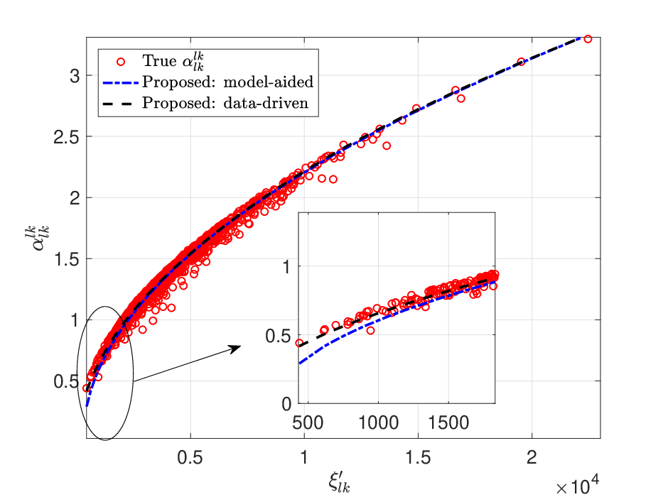
To provide more insights into the properties of the proposed estimators, Fig. 11 shows one feature of the input data, namely , versus the true value of . We consider one user (i.e., one large-scale realization) and small-scale realization for MR precoding and . While these data points are represented by 1000 circles, the lines represent the estimate of that the two proposed estimators are providing for each value of . Note that the two estimators provide deterministic mappings while the true relationship is random since the data are random (as is always the case in estimation theory). We can see that the proposed estimators provide almost the same estimate when is large, while there is a gap between the estimators when is small. The reason that the data-driven estimator obtains a better mapping than the model-based estimator is that it is trained for a system with finite and , while the model-aided estimator is obtained from asymptotic arguments. Hence, the data-driven estimator provides lower NMSE and SE in the considered setup where is small.
Fig. 12 shows the impact of the spatial correlation level, which is expressed by the ASD. A small ASD represents high spatial correlation, and vice versa. The NMSE produced by the hardening bound is heavily depending on the strength of the spatial correlation. Specifically, the NMSE is quite high with a low ASD value (i.e., strong spatial correlation) since the channel vectors are less hardened. The approximation by the hardening bound becomes more accurate as the ASD increases (i.e., the channels approach spatially uncorrelated fading). In contrast, it is worth to notice that the proposed model-based approach is almost insensitive to the spatial correlation and close to the optimistic solution in the limiting regime when .


VII Conclusion
This paper presented a model- and data-driven-based approach for downlink channel estimation in a multi-cell Massive MIMO system. The effective channel gains facilitate decoding of the desired signal from the received data signal at the users. The typical approach in Massive MIMO literature is to use the mean of effective channel gains as a piece of legitimate information for decoding. Using the mean of effective channel gains is a perfect assumption for hardening channels. If the channel hardening level is low, the performance fluctuation is high when using mean values. We investigate the performance for both having channel hardening and low level of channel hardening conditions. We derived closed-form expressions for the downlink channel gain using MR and ZF precoding at BSs for uncorrelated Rayleigh fading channels for the model-based approach. Furthermore, we provided a closed-form expression MR precoding for the correlated Rayleigh channel model. In addition, we proposed a second method that is data-driven and trains a neural network to identify a mapping between the available information and the effective channel gain. Moreover, we present a performance comparison of the proposed model- and data-driven-based methods in terms of NMSE and per-user SE. The results highlight the superior performance of our proposed approaches in SE, specifically correlated fading, i.e., when the hardening level is low.
Several of the proofs in this appendix make uses of the weak law-of-large-numbers, which can be stated as follows.
Lemma 8.
Let be a sequence of independent and identically distributed random variables with mean value and bounded variance [39, Ch. 2]. It then follows that
| (44) |
-A Proof of Lemma 2
Let denote the portion of each coherence interval dedicated to data transmission and notice that we consider the limit where . We can then rewrite (15) as
| (45) | ||||
As , it follows from Lemma 8 that the second and third terms in (45) converges to zero. Moreover, the fourth term converges to its mean value . Therefore, (45) simplifies asymptotically to
| (46) |
It remains to determine an asymptotic equivalent expression for . To this end, let us introduce a new variable and expand as
| (47) |
Let denote the expectation with respect to the random data signals and noise (i.e., the conditional expectation given the channel realizations). Since all the cross-terms between different have zero mean, it follows that
-B Proof of Lemma 3
We first reformulate (16) by dividing both sides by to obtain an asymptotic equivalence
| (50) |
as . At the right-hand side of (50), is a scaled-down version of the intra-cell interference and is further reformulated by adding and subtracting the mean value of as
| (51) |
where has zero mean and comes from a common distribution with bounded variance. Hence, in the asymptotic regime where (in the way stated in the lemma), . Note that the expectations are with respect to the channel realizations, while the convergence in probability considers both user locations and channel realizations. It then follows from Lemma 8 that
| (52) |
In addition, is a scaled-down version of inter-cell interference. By following a similar approach (with a fixed number of cells), is reformulated as
| (53) |
where have zero mean and come from a common distribution with bounded variance. As (in the way stated in the lemma), it follows that which implies
| (54) |
By using the asymptotic equivalences provided in (52) and (54) in (50), we provide the expression given in (17).
References
- [1] A. Ghazanfari, T. Van Chien, E. Bjornson, and E. G. Larsson, “Learning to perform downlink channel estimation in massive mimo systems,” in 2021 17th International Symposium on Wireless Communication Systems (ISWCS). IEEE, 2021, pp. 1–6.
- [2] E. G. Larsson, O. Edfors, F. Tufvesson, and T. L. Marzetta, “Massive MIMO for next generation wireless systems,” IEEE Commun. Mag., vol. 52, no. 2, pp. 186–195, 2014.
- [3] S. Parkvall, E. Dahlman, A. Furuskär, and M. Frenne, “NR: The new 5G radio access technology,” IEEE Communications Standards Magazine, vol. 1, no. 4, pp. 24–30, 2017.
- [4] T. L. Marzetta, “Noncooperative cellular wireless with unlimited numbers of base station antennas,” IEEE Trans. Wireless Commun., vol. 9, no. 11, pp. 3590–3600, 2010.
- [5] E. Björnson, J. Hoydis, and L. Sanguinetti, Massive MIMO Networks: Spectral, Energy, and Hardware Efficiency. Now Publishers, Inc., 2017, vol. 11, no. 3-4.
- [6] J. Jose, A. Ashikhmin, T. L. Marzetta, and S. Vishwanath, “Pilot contamination and precoding in multi-cell TDD systems,” IEEE Trans. Wireless Commun., vol. 10, no. 8, pp. 2640–2651, 2011.
- [7] H. Yang and T. L. Marzetta, “Performance of conjugate and zero-forcing beamforming in large-scale antenna systems,” IEEE J. Sel. Areas Commun., vol. 31, no. 2, pp. 172–179, 2013.
- [8] T. L. Marzetta, E. G. Larsson, H. Yang, and H. Q. Ngo, Fundamentals of Massive MIMO. Cambridge University Press, 2016.
- [9] S. Gunnarsson, J. Flordelis, L. V. der, and F. Tufvesson, “Channel hardening in massive MIMO: Model parameters and experimental assessment,” IEEE Open Journal of the Communications Society, vol. 1, pp. 501–512, 2020.
- [10] H. Q. Ngo and E. G. Larsson, “No downlink pilots are needed in TDD massive MIMO,” IEEE Trans. Wireless Commun., vol. 16, no. 5, pp. 2921–2935, 2017.
- [11] H. Q. Ngo, E. G. Larsson, and T. L. Marzetta, “Massive MU-MIMO downlink TDD systems with linear precoding and downlink pilots,” in Proc. Annual Allerton Conf. on Commun., Cont., and Comp. IEEE, 2013, pp. 293–298.
- [12] H. Q. Ngo and E. G. Larsson., “Blind estimation of effective downlink channel gains in massive MIMO,” in Proc. IEEE Int. Conf. on Acoustics, Speech, and Signal Process. (ICASSP). IEEE, 2015, pp. 2919–2923.
- [13] P. Pasangi, M. Atashbar, and M. M. Feghhi, “Blind downlink channel estimation of multi-user multi-cell massive MIMO system in presence of the pilot contamination,” AEU-International Journal of Electronics and Communications, vol. 117, p. 153099, 2020.
- [14] R. R. Müller, L. Cottatellucci, and M. Vehkaperä, “Blind pilot decontamination,” IEEE J. Sel. Topics Signal Process., vol. 8, no. 5, pp. 773–786, 2014.
- [15] E. Amiri, R. R. Müller, and W. Gerstacker, “Blind pilot decontamination in massive MIMO by independent component analysis,” in Proc. IEEE Globecom Workshops (GC Wkshps). IEEE, 2017, pp. 1–5.
- [16] K. Ghavami and M. Naraghi-Pour, “Blind channel estimation and symbol detection for multi-cell massive MIMO systems by expectation propagation,” IEEE Trans. Wireless Commun., vol. 17, no. 2, pp. 943–954, 2017.
- [17] C. Shin, R. W. Heath, and E. J. Powers, “Blind channel estimation for MIMO-OFDM systems,” IEEE Trans. Veh. Technol., vol. 56, no. 2, pp. 670–685, 2007.
- [18] E. de Carvalho and D. T. Slock, “Asymptotic performance of ML methods for semi-blind channel estimation,” in Proc. IEEE Asilomar Conf. Signals, Systems, and Computers, vol. 2. IEEE, 1997, pp. 1624–1628.
- [19] E. D. Carvalho and D. T. Slock, “Cramer-Rao bounds for semi-blind, blind and training sequence based channel estimation,” in Proc. IEEE Workshop on Signal Processing Adv. in Wireless Commun. (SPAWC). IEEE, 1997, pp. 129–132.
- [20] T. O’Shea and J. Hoydis, “An introduction to deep learning for the physical layer,” IEEE Transactions on Cognitive Communications and Networking, vol. 3, no. 4, pp. 563–575, 2017.
- [21] T. V. Chien, T. N. Canh, E. Björnson, and E. G. Larsson, “Power control in cellular massive MIMO with varying user activity: A deep learning solution,” IEEE Trans. Wireless Commun., vol. 19, no. 9, pp. 5732–5748, 2020.
- [22] L. Sanguinetti, A. Zappone, and M. Debbah, “Deep learning power allocation in massive MIMO,” in Proc. IEEE Asilomar Conf. Signals, Systems, and Computers. IEEE, 2018, pp. 1257–1261.
- [23] M. Sadeghi and E. G. Larsson, “Adversarial attacks on deep-learning based radio signal classification,” IEEE Wireless Commun. Lett., vol. 8, no. 1, pp. 213–216, 2018.
- [24] H. Sun, X. Chen, Q. Shi, M. Hong, X. Fu, and N. D. Sidiropoulos, “Learning to optimize: Training deep neural networks for interference management,” IEEE Trans. Signal Process., vol. 66, no. 20, pp. 5438–5453, 2018.
- [25] Ö. T. Demir and E. Björnson, “Channel estimation under hardware impairments: Bayesian methods versus deep learning,” in Proc. Int. Symp. of Wireless Communication Systems (ISWCS). IEEE, 2019, pp. 193–197.
- [26] E. Björnson and P. Giselsson, “Two applications of deep learning in the physical layer of communication systems [lecture notes],” IEEE Signal Process. Mag., vol. 37, no. 5, pp. 134–140, 2020.
- [27] A. Balatsoukas-Stimming and C. Studer, “Deep unfolding for communications systems: A survey and some new directions,” in IEEE International Workshop on Signal Processing Systems (SiPS), 2019, pp. 266–271.
- [28] F. Sohrabi, K. M. Attiah, and W. Yu, “Deep learning for distributed channel feedback and multiuser precoding in FDD massive MIMO,” IEEE Trans. Wireless Commun., vol. 20, no. 7, pp. 4044–4057, 2021.
- [29] L. Sanguinetti, E. Björnson, and J. Hoydis, “Towards massive MIMO 2.0: Understanding spatial correlation, interference suppression, and pilot contamination,” IEEE Trans. Commun., vol. 68, no. 1, pp. 232–257, 2020.
- [30] E. Björnson, J. Hoydis, and L. Sanguinetti, “Massive MIMO has unlimited capacity,” IEEE Trans. Wireless Commun., vol. 17, no. 1, pp. 574–590, Jan. 2018.
- [31] S. M. Kay, Fundamentals of statistical signal processing. Prentice-Hall, 1993.
- [32] T. L. Marzetta, “How much training is required for multiuser MIMO?” in Proc. IEEE Asilomar Conf. Signals, Systems, and Computers, 2006, pp. 359–363.
- [33] J. Hoydis, S. ten Brink, and M. Debbah, “Massive MIMO in the UL/DL of cellular networks: How many antennas do we need?” IEEE J. Sel. Areas Commun., vol. 31, no. 2, pp. 160–171, 2013.
- [34] I. Goodfellow, Y. Bengio, A. Courville, and Y. Bengio, Deep learning. MIT press Cambridge, 2016, vol. 1, no. 2.
- [35] K. Hornik, M. Stinchcombe, H. White et al., “Multilayer feedforward networks are universal approximators.” Neural networks, vol. 2, no. 5, pp. 359–366, 1989.
- [36] D. P. Kingma and J. Ba, “Adam: A method for stochastic optimization,” 2017.
- [37] L. Sanguinetti, E. Björnson, and J. Hoydis, “Toward massive MIMO 2.0: Understanding spatial correlation, interference suppression, and pilot contamination,” IEEE Trans. Commun., vol. 68, no. 1, pp. 232–257, 2019.
- [38] H. Yang and T. L. Marzetta, “Massive MIMO with max-min power control in line-of-sight propagation environment,” IEEE Trans. Commun., vol. 65, no. 11, pp. 4685–4693, 2017.
- [39] S. M. Ross, Introduction to probability models. Academic press, 2014.