“Worst-Case” Micro-Lensing in the Identification and Modeling of Lensed QuasarsJournal: ApJ
Abstract
Although micro-lensing of macro-lensed quasars and supernovae provides unique opportunities for several kinds of investigations, it can add unwanted and sometimes substantial noise. While micro-lensing flux anomalies may be safely ignored for some observations, they severely limit others. “Worst-case” estimates can inform the decision whether or not to undertake an extensive examination of micro-lensing scenarios. Here, we report “worst-case” micro-lensing uncertainties for point sources lensed by singular isothermal potentials, parameterized by a convergence equal to the shear and by the stellar fraction. The results can be straightforwardly applied to non-isothermal potentials utilizing the mass sheet degeneracy. We use micro-lensing maps to compute fluctuations in image micro-magnifications and estimate the stellar fraction at which the fluctuations are greatest for a given convergence. We find that the worst-case fluctuations happen at a stellar fraction . For macro-minima, fluctuations in both magnification and demagnification appear to be bounded (, where is magnitude relative to the average macro-magnification). Magnifications for macro-saddles are bounded as well (). In contrast, demagnifications for macro-saddles appear to have unbounded fluctuations as and .
Keywords:
Gravitational microlensing, Quasar micro-lensing, Strong gravitational lensingI Introduction
Gravitational lensing has emerged as a powerful tool to probe the potentials of distant galaxies and galaxy clusters, and has further been used to help constrain models of dark matter and dark energy. Lensed quasars have been particularly prominent, and the number of known quadruply lensed quasars has increased by roughly 50% since the first data release from the Gaia satellite (Gaia Collaboration et al. 2016). Approximately 20 quadruply lensed quasars have been discovered using Gaia DR1 and DR2, often in concert with other catalogs.
The Gaia GraL group (Krone-Martins et al. 2018) identified 80,000 quartets of candidate point sources for consideration as possible quadruply lensed quasars. The positions and fluxes were analyzed, with great success, using “Extremely Randomized Trees” (Delchambre et al. 2019), with twelve out of thirteen known quadruply lensed quasars with four catalogued images ranked in the top 0.6%. The authors attribute the ranking of the thirteenth, 3 times further down the list, to micro-lensing of the quasar images by stars in the lensing galaxy, a phenomenon that had not been taken into account in their training set of roughly systems.
Micro-lensing helps place constraints on the smooth (dark) matter content of the lensing galaxy. Previous work has shown that, for highly magnified macro-images, the fluctuations in flux ratio due to micro-lensing often increases with the introduction of dark matter to the lens model (Schechter & Wambsganss 2002). Furthermore, it is expected that these micro-lensing fluctuations are larger for saddle-points as compared to minima (Witt et al. 1995), which large-scale parameter studies of micro-lensing magnification probability distributions have confirmed (Wambsganss 1992; Lewis & Irwin 1995; Vernardos & Fluke 2013). Contingent upon available resources, it would be possible to include the effects of micro-lensing in the training set of the Extremely Randomized Trees, particularly with the public availability of the GERLUMPH suite of simulations (Vernardos et al. 2014). Here we describe an approximate alternative that could be readily adapted to lens searches, which inevitably involve expectations for lensed flux ratios.
Briefly, we assume a convergence and shear appropriate to a singular isothermal elliptical potential – a model that works reasonably well for most know quadruply lensed quasar systems – and search for the stellar contribution to the convergence that produces the largest micro-lensing fluctuations for a point source. We call this “worst-case” micro-lensing, and give the 95% confidence range for the fluctuations. One can then use these ranges (accounting in some way for the likelihood of the worst case stellar fraction) to assign a likelihood to a discrepant source flux. The modeling of Gaia quartets is just one of many lens modeling problems where worst case estimates could prove useful. One needn’t completely discount the observed fluxes from quasar images if expected fluctuations are small, as for low magnification images (particularly macro-minima, which as stated previously suffer less from such fluctuations than macro-saddles).
The fluctuations discussed within this work are for that fraction of the source that can be treated as pointlike. Our discussions are not relevant to the flux from more extended regions of emissions corresponding to longer wavelength observations, which have narrower magnification distributions (Bate et al. 2007).
The organization of this paper is as follows: In §II, we give a brief introduction to gravitational lensing, macro-lensing models, and the phenomenon of micro-lensing. In §III, we describe the important components of our methodology, including the micro-lensing maps upon which our analyses depended. §IV shows our results, including plots of worst-case fluctuations. A set of systems which showcase “worst-case” conditions are discussed in §V. Conclusions are presented in §VI.
II Background
II.1 Gravitational Lensing Phenomenon
Gravitational lensing is a direct consequence of general relativity. Light passing near a massive object is deflected, much as a light ray obeying Fermat’s principle of least time refracts on passing through an optical lens. Gravitational lensing can be succinctly described using the time delay surface
| (1) |
where is the redshift of the lens, , , and are the angular diameter distances from the observer to lens, observer to source, and lens to source respectively, is the position in the source plane, is the position in the image plane, and
| (2) |
is the Newtonian gravitational potential of the lens scaled and integrated along the line of sight (Schneider et al. 1992). The lens equation, which can be simply written as
| (3) |
or more fully as
| (4) |
provides the locations where images of the source are seen – at stationary points of the time delay surface, which can be either minima, maxima, or saddle-points. The magnifications of the images are inversely proportional to the curvature of the time delay surface.
The lens equation can be non-dimensionalized into
| (5) |
where is the position in the source plane, is the position in the image plane, and is the gravitational potential. The magnifications of the images are then
| (6) |
with the sign of the magnification determining the parity of the image. Saddle-points have , while minima and maxima have . Furthermore, minima are always magnified, whereas saddles and maxima can be demagnified.



II.2 Quadruple Lenses and Macro-lensing Models
Our analysis is appropriate to lensed sources with any number of images, but as quadruply lensed sources have greater redundancy, we concentrate on these. Quadruply lensed quasars play an important role in extragalactic astrophysics, helping elucidate the potentials, stellar content, and dark matter content of the lensing galaxy as well as structural properties of the background source (Schechter & Wambsganss 2004; Bate et al. 2008). Furthermore, quadruple lenses are of great importance in cosmology because they help constrain the values of parameters such as the Hubble constant (Suyu et al. 2013). Lensing galaxies are often modeled as singular isothermal elliptical potentials (SIEP) (Kovner 1987), for which observable images are seen at saddle-points and minima of the light travel time surface. An image also forms at the maximum near the center of the lens’ matter distribution, but the singular nature of the SIEP model at this location means that this image is infinitely demagnified. This model has been reasonably successful at predicting the image positions (Schechter & Wynne 2019). The magnifications of the macro-images can be computed as as
| (7) |
where denotes the effective convergence of the lens at the position of a macro-image and denotes its shear. is related to the gravitational potential through the two-dimensional Poisson equation
| (8) |
while with
| (9) |
Minima of the time delay surface occur when , saddle-points occur when , and maxima occur when .
For isothermal gravitational potentials, we further have , for which equation (7) reduces to
| (10) |
II.3 Micro-lensing
“Micro-lensing” is distinguished from “macro-lensing” in that the multiple images produced by the former cannot be resolved with today’s telescopes. Both can occur simultaneously, as when a galaxy produces multiple observable images of a quasar and the stars within the galaxy produce unresolved multiples of those images. It is useful to distinguish between micro-lensing at low optical depth, in which a single star does the lensing, and lensing at high optical depth, when a great many stars contribute to the lensing, producing a great many micro-images (Paczynski 1986). The observed flux from the macro-image is then the combined flux from the micro-images.
As the source and the micro-lensing stars move, the micro-images change in brightness, introducing fluctuations in the observed fluxes of macro-images. As one might expect, this effect depends on the stellar content of the lens. For this reason we define the stellar fraction as
| (11) |
where is the convergence due to stars, is the convergence due to smooth matter, and is the total convergence.
III Method
III.1 Micro-lensing Maps
Our work is based on micro-lensing magnification maps created using the inverse ray-shooting technique (Schneider & Weiss 1986; Kayser et al. 1986). A multitude of light rays are traced backwards with the lens equation from image plane to source plane and collected in a pixelated map. The number of rays per pixel is then proportional to the total magnification. The dimensionless lens equation is given by
| (12) |
where is the mass of a micro-lens in units of some mass that determines the Einstein radius , and is the position of a micro-lens. For all of our simulations, we took our stars to be of unit mass and used the corresponding as our unit distance.


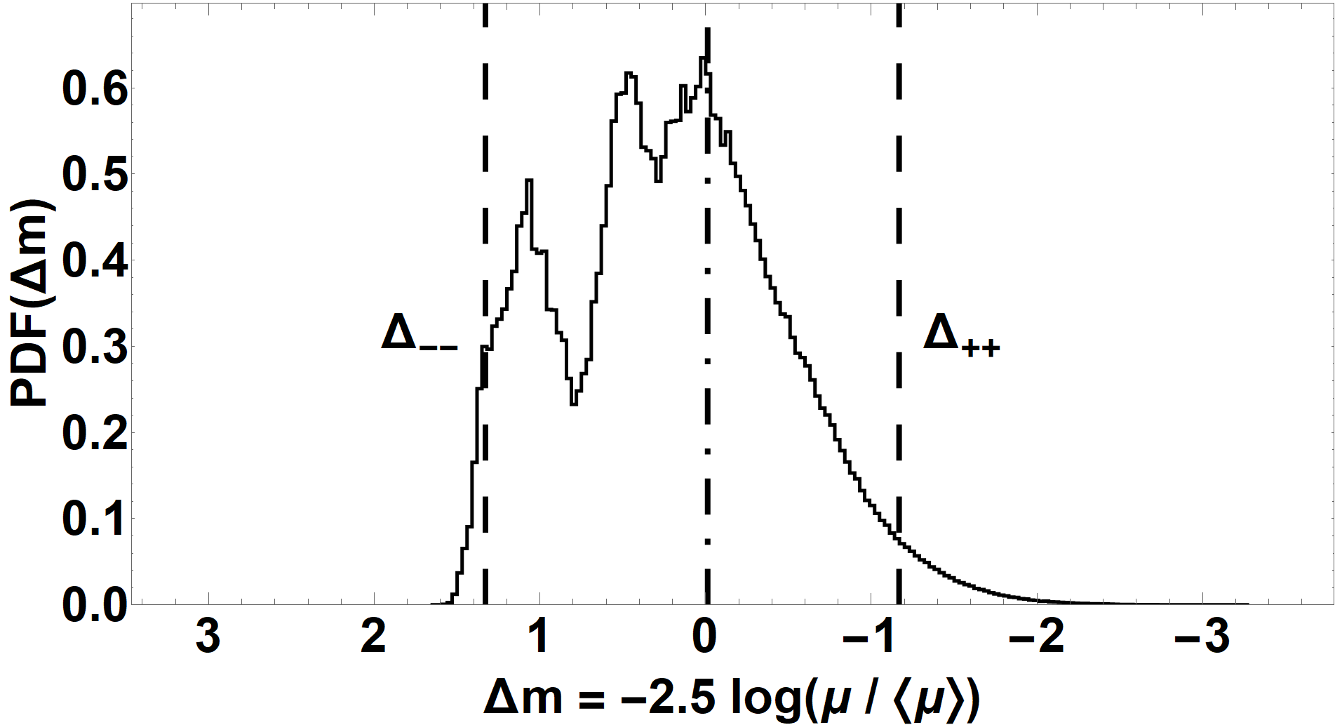
Our investigation initially used the publicly available magnification maps of the GERLUMPH Data Release 1 (Vernardos et al. 2014), although we ultimately ended up using our own ray-shooting code that runs on a Graphics Processing Unit (GPU) to more easily examine areas of interest in the high magnification, low stellar density regime while maintaining a set of consistent simulation parameters such as map size and average ray density where possible. Our GPU implementation is neither a fully direct ray-tracing like that of Thompson et al. 2010, nor a fully GPU parallelized tree-code like that of Alpay 2019. Instead, our naive implementation uses all the stars in the field to directly shoot 4 rays (one near each of the corners) in each square of a grid that constitutes the shooting region in the image plane. We calculate Taylor coefficients of the deflection angle (up to third order) within the square and use those coefficients to then shoot more rays within the square. The size of the squares depends on the number density of rays in the image plane, which itself depends on the macro-magnification , the desired average number of rays per pixel , the pixel size, and the number of rays that are shot using the Taylor coefficients. We note that the sizes of the squares in the image plane were never greater than for our simulations, with the majority being less than over the parameter space sampled. The top portion of Figure 1 shows sample magnification maps created with our code. We shot rays into a square in the source plane with a side length of and pixels, so that each pixel is a x square. We additionally chose for all of our simulations.
III.2 Worst-Case Analysis
The magnification maps show the total source magnification as a function of position. The magnification at a specific source position is the sum of the magnifications of the many micro-images, and in general will fluctuate around the average macro-magnification as the source moves. We create histograms of the magnifications, expressed as magnitude differences from the theoretical average , using
| (13) |
We choose to examine worst-case micro-lensing by calculating the and percentiles11 1 Chosen to reflect a quasi- 2 standard deviation spread of the magnitude distributions; i.e., we find the ray counts for which of all the pixels contain more rays and for which of all the pixels contain fewer rays, and transform them into magnitudes. We designate these limits by and respectively.22 2 We use and to refer to the cutoffs as well as to the number of rays, the magnification, and the magnitude at those cutoffs, for ease of reference. Which quantity is meant at a particular time should be evident by context. The bottom portion of Figure 1 shows the histograms for the magnification maps of the top portion, with the values of and marked. For every point sampled in space, we run 10 micro-lensing simulations and calculate the average and from these 10 simulations.
III.3 The Mass-Sheet Degeneracy
The mass sheet degeneracy (Falco et al. 1985) allows for an arbitrary scaling of lens mass distributions without affecting any of the observable quantities like position and magnification. In the context of micro-lensing, this degeneracy allows for any triplet of to be converted into an effective doublet33 3 The choice of doublet is arbitrary. A common alternative is to choose . through a judicious choice of effective , reducing the parameter space by one dimension while scaling the magnifications and source plane coordinates (Paczynski 1986; Kochanek 2004; Vernardos et al. 2014; Schechter et al. 2014). Our simulations, which sample the parameter space of within the square where and , are immediately applicable to the SIEP model. However, they are still relevant for a wider range of parameter values when appropriately scaled. More specifically, given values for , the transformations
| (14) |
| (15) |
and
| (16) |
allow comparison with our results.
IV Results
We created contour plots of our averaged and as functions of .44 4 Contour plots were created using Mathematica’s ListContourPlot function. They are simple linear interpolations of the data points provided. The left half of Figure 2 shows , while the right half shows . The “+” symbols on the plots denote the points in the parameter space for which we ran micro-lensing simulations. Data points are symmetrical around for the majority of the plots, with the symmetry broken closer to to explore regions of interest. The top portions of the plots show the entirety of the parameter space sampled, while the bottom portions of the plots shows a zoom around for low values of .
IV.1
The plot of displays several interesting properties. First, for both macro-minima (the left half, ) and macro-saddles (the right half, ), there appears to be a ridge along which the value of is extremized. For each respective macro-image type, the brightest value of appears to be constant along this ridge. For macro-minima we found this value to be mag, while for macro-saddles we found mag. The dashed black line on the plot denotes the locus where , which traces the ridge of brightest . Figure 3 displays the values of along this ridge.
IV.2
The left half of Figure 2 shows the contour plot for . Note the difference in the range of magnitudes shown compared to that of . The contours of this plot are markedly different than that of , and display different features for macro-minima as opposed to macro-saddles. For the macro-minima, there again appears to be a ridge along which the value of is extremized. We find this extremal value to be mag. The dashed black line no longer describes where this ridge is located though – the ridge appears to have some other locus describing it.
The macro-saddles have no such ridge where is extremized; instead, values form a ‘basin’ with slowly sinking contours that grow fainter and fainter. However, for a given vertical cut at a specific value, the value of grows fainter as increases before reaching an extremum and growing brighter again. This faintest value for a specific is described once more by the locus where . As and , the contours of slowly sink down further and further, the dimmest possible fluctuations becoming fainter and fainter as the macro-image becomes brighter and the stars farther apart. We were limited by computer power and time, but we found values of the demagnification up to mag in this regime.

IV.3 Simulation Errors and Uncertainties
Appendix A contains a discussion of some of the errors associated with micro-lensing simulations, our mitigations of such errors, and the uncertainties in our measured values for and .
V Observed “Worst” Cases
“Worst-case” scenarios require the confluence of three factors: the random configuration of micro-lensing stars, the ratio of stellar to total mass surface density, and the ratio of the half-light radius of the source to the Einstein ring radius of the micro-lenses. Likelihoods for the last two of these will vary from one circumstance to another. There are many quadruply lensed sources for which the observed flux ratio anomalies at one or another wavelength are much smaller than the worst case, either by virtue of the source size or the micro-lens surface density. In this section we examine three examples of lensed systems that are consistent with a worst case scenario.
V.1 Quad Lens RX J1131-1231
The quad RX J1131-1231 was the thirteenth and last ranked GraL system described in §1. We have used Keeton’s lensmodel program (Keeton 2001) to model HST positions for the four images as a singular isothermal sphere with external shear.
Minimizing the RMS residuals of Gaia magnitudes from the model predictions, we find that image C, the faintest of the cusp images, is 0.34 magnitudes fainter than predicted. This is only 1/4 of the excursion shown in Figure 2. Image D, isolated on the far side of the lens, is 1.20 magnitudes brighter than predicted. This is roughly 3/4 of the excursion shown in 2.
These fluctuations are not extreme. It raises the question of why the other twelve known lenses exhibited fluctuations that were so much smaller. The widely appreciated answer is that the optical continuum emitting regions of quasars are at least as extended as the Einstein rings of micro-lensing stars. Pooley et al. 2007 show that the rms deviations of optical fluxes from those predicted by lens models only are half as large as those observed in X-ray fluxes, which have been found to arise from smaller regions than the optical (Morgan et al. 2008).
V.2 Quad Lens SDSS J0924+0219
Keeton et al. 2006 call SDSS J0924+0219 “the most anomalous lensed quasar”. Using the Keeton et al. model, with the HST V band source flux determined from the B and C images, we find the D image is 2.79 magnitudes fainter than predicted, compared with a excursion of 3.1 mag found from Figure 3. Using the X-ray fluxes from Pooley et al. 2007 again calibrated by B and C, we find image D is 2.58 magnitudes fainter than predicted.
One might wonder whether the faintness of image D is due to substructure milli-lensing, but Badole et al. 2020 have found radio flux ratios that are consistent with the model predictions, ruling out the milli-lensing hypothesis. SDSS J0924+0219 would appear to be a quad in which our worst case estimate is borne out.
V.3 SN Ia iPTF16geu
Mörtsell et al. 2020 present a model for the observations of the quadruply lensed supernovae iPTF16geu. Though slightly shallower than isothermal, we use their magnifications to compute the isothermal effective . Their image 1 is 1.00 mag brighter than the model prediction and their image 4 is 0.70 mag fainter than predicted. Their estimated stellar fraction is . Figure 2 give mag and mag. Taken together the fluctuations are roughly what one would expect if the supernova were pointlike at the time of observation.
VI Conclusions
We have conducted an analysis of the effects of micro-lensing on the brightness of gravitationally lensed images. We used micro-lensing maps to obtain “worst-case” uncertainties (which we defined as the boundaries of the 95% confidence range) in the micro-magnification for different combinations of the convergence and stellar fraction of lenses characterized by isothermal potentials where . On the faint end (), demagnification can be attributed to the absence of extra image pairs – a macro-minimum has only one micro-minimum and a saddle-point for every star, while a macro-saddle has one micro-saddle corresponding to the global saddle-point and fainter micro-saddles for every star. The fact that minima must be of at least unit magnification while saddle-points can be arbitrarily demagnified leads to some of the differences between the left and right half of the plot in Figure 2. At the bright end (), high magnifications are largely due to caustic crossing events or passage near cusps. The bottom half of Figure 1 shows the magnification maps of the top half converted into a 3 color scheme: black for , white for , and gray for our 95% interval in between. The caustics largely occur within the region of , and would be completely recovered in white in the figure if pixel resolution was increased.
While our purpose was determining the “worst-case” micro-lensing fluctuations, we can comment on the cause of deviations within the 95% confidence range as well. Deviations within can, for the most part, be attributed to variations in the number of micro-minima. Granot et al. 2003 assert that these variations are greatest when the average number of extra image pairs . If the average area of the caustic due to a star scales with then the covering factor of the caustics, which gives the expected number of extra image pairs, that maximizes the variations can be roughly found as , which recovers the locus . Alternatively, one can consider the contributions of smooth and grainy matter to the magnification tensor. The stars introduce fluctuations into the magnification tensor on top of the smooth matter component. One might expect these fluctuations to be most impactful when , which (for macro-saddles at least) recovers as well.
The appendix of Liao et al. 2015 examines the role of in the RMS fluctuations of magnification maps for a macro-minimum and a macro-saddle. For their macro-minimum, which has and , we would expect the the fluctuations to peak at . Accounting for the somewhat sparse sampling in their Figure 14, we find this value of to be consistent with their results. Similarly for their macro-saddle, which has and resulting in the same macro-magnification, a peak in the RMS near is clearly seen. Indeed Figure 14 of Liao et al. 2015, after appropriate conversion using the mass-sheet degeneracy, bears a striking resemblance to a vertical cut of or in our Figure 2 at or (for the minimum or saddle respectively).
Under the worst set of conditions corresponding to micro-lensing of a highly magnified saddle with low stellar surface mass density, our analysis showed that micro-lensing introduces uncertainties of at least three magnitudes, with the uncertainty appearing to increase unbounded as and . Elsewhere, (de)magnifications appear to be bounded. Fluctuations in the magnification for macro-minima and macro-saddles peak when the stellar fraction .
Simple comparisons of observed magnitude differences in lensed systems to the “worst-case” fluctuations in Figure 2 can serve as a guide in determining whether more detailed micro-lensing analyses are worthwhile.
Appendix A Simulation Errors and Uncertainties
Any micro-lensing ray tracing simulations are subject to the effects of using a finite number of stars. Rays passing close to a star are deflected out of the receiving square, but there are no stars far away which deflect rays in. Katz et al. 1986 and Schneider & Weiss 1987 provide expressions for the number of stars seen in a solid angle containing a desired percentage of the total flux; our code uses enough stars and appropriately sized shooting regions to account for 99% of the flux.
Any given realizations of a star field will still exhibit slight differences from one another as well. Our decision to average over 10 simulations for each point in attempts to mitigate such differences. Figure 2 shows the average and from each set of 10 simulations. Here, we discuss the spread of each set.
What we actually measure are the number of rays corresponding to our and limits in each simulation, so the standard deviation of each set of 10 simulations is found in units of the number of rays as well. We must then account for the fact that is demagnified and will have fewer rays than the magnified – a standard deviation of 10 rays for is not necessarily better than a standard deviation of 100 rays for . The obvious comparators for and are the number of rays giving the or limits themselves. Figure 4 shows density plots of the uncertainties in the number of rays for and measured relative to themselves. We find that for the majority of the parameter space covered. This increases slightly to closer to , particularly for higher values of . There are some additional instances where for much lower values of , but these can be attributed to the low surface mass density and the fact that our source plane region of is likely somewhat smaller than necessary to adequately sample the caustics. We find that for the entirety of the parameter space, with the majority having .


We note here that our choice of plays a role in the errors. For low macro-magnifications, this choice of is more than adequate, but for high macro-magnifications a larger number of rays may have been more appropriate (at the expense of more computing time). Some of our magnification maps contained pixels with zero rays, although unsurprisingly this only occurred in the high macro-magnification, low stellar density regime of the macro-saddles where there is the possibility of strong demagnification. Increasing the average number of rays would have removed any 0 count pixels and decreased our uncertainties relative to .
References
- Alpay (2019) Alpay, A. 2019, Teralens. https://github.com/illuhad/teralens
- Badole et al. (2020) Badole, S., Jackson, N., Hartley, P., et al. 2020, MNRAS, 496, 138, doi: 10.1093/mnras/staa1488
- Bate et al. (2008) Bate, N. F., Floyd, D. J. E., Webster, R. L., & Wyithe, J. S. B. 2008, MNRAS, 391, 1955, doi: 10.1111/j.1365-2966.2008.14020.x
- Bate et al. (2007) Bate, N. F., Webster, R. L., & Wyithe, J. S. B. 2007, MNRAS, 381, 1591, doi: 10.1111/j.1365-2966.2007.12330.x
- Delchambre et al. (2019) Delchambre, L., Krone-Martins, A., Wertz, O., et al. 2019, A&A, 622, A165, doi: 10.1051/0004-6361/201833802
- Falco et al. (1985) Falco, E. E., Gorenstein, M. V., & Shapiro, I. I. 1985, ApJ, 289, L1, doi: 10.1086/184422
- Gaia Collaboration et al. (2016) Gaia Collaboration, Brown, A. G. A., Vallenari, A., et al. 2016, A&A, 595, A2, doi: 10.1051/0004-6361/201629512
- Granot et al. (2003) Granot, J., Schechter, P. L., & Wambsganss, J. 2003, ApJ, 583, 575, doi: 10.1086/345447
- Katz et al. (1986) Katz, N., Balbus, S., & Paczynski, B. 1986, ApJ, 306, 2, doi: 10.1086/164313
- Kayser et al. (1986) Kayser, R., Refsdal, S., & Stabell, R. 1986, A&A, 166, 36
- Keeton (2001) Keeton, C. R. 2001, arXiv e-prints, astro. https://arxiv.org/abs/astro-ph/0102340
- Keeton et al. (2006) Keeton, C. R., Burles, S., Schechter, P. L., & Wambsganss, J. 2006, ApJ, 639, 1, doi: 10.1086/499264
- Kochanek (2004) Kochanek, C. S. 2004, ApJ, 605, 58, doi: 10.1086/382180
- Kovner (1987) Kovner, I. 1987, ApJ, 312, 22, doi: 10.1086/164846
- Krone-Martins et al. (2018) Krone-Martins, A., Delchambre, L., Wertz, O., et al. 2018, A&A, 616, L11, doi: 10.1051/0004-6361/201833337
- Lewis & Irwin (1995) Lewis, G. F., & Irwin, M. J. 1995, MNRAS, 276, 103, doi: 10.1093/mnras/276.1.103
- Liao et al. (2015) Liao, K., Treu, T., Marshall, P., et al. 2015, ApJ, 800, 11, doi: 10.1088/0004-637X/800/1/11
- Morgan et al. (2008) Morgan, C. W., Kochanek, C. S., Dai, X., Morgan, N. D., & Falco, E. E. 2008, ApJ, 689, 755, doi: 10.1086/592767
- Mörtsell et al. (2020) Mörtsell, E., Johansson, J., Dhawan, S., et al. 2020, MNRAS, 496, 3270, doi: 10.1093/mnras/staa1600
- Paczynski (1986) Paczynski, B. 1986, ApJ, 301, 503, doi: 10.1086/163919
- Pooley et al. (2007) Pooley, D., Blackburne, J. A., Rappaport, S., & Schechter, P. L. 2007, ApJ, 661, 19, doi: 10.1086/512115
- Schechter et al. (2014) Schechter, P. L., Pooley, D., Blackburne, J. A., & Wambsganss, J. 2014, ApJ, 793, 96, doi: 10.1088/0004-637X/793/2/96
- Schechter & Wambsganss (2002) Schechter, P. L., & Wambsganss, J. 2002, ApJ, 580, 685, doi: 10.1086/343856
- Schechter & Wambsganss (2004) Schechter, P. L., & Wambsganss, J. 2004, in Dark Matter in Galaxies, ed. S. Ryder, D. Pisano, M. Walker, & K. Freeman, Vol. 220, 103. https://arxiv.org/abs/astro-ph/0309163
- Schechter & Wynne (2019) Schechter, P. L., & Wynne, R. A. 2019, ApJ, 876, 9, doi: 10.3847/1538-4357/ab1258
- Schneider et al. (1992) Schneider, P., Ehlers, J., & Falco, E. E. 1992, Gravitational Lenses, doi: 10.1007/978-3-662-03758-4
- Schneider & Weiss (1986) Schneider, P., & Weiss, A. 1986, A&A, 164, 237
- Schneider & Weiss (1987) —. 1987, A&A, 171, 49
- Suyu et al. (2013) Suyu, S. H., Auger, M. W., Hilbert, S., et al. 2013, ApJ, 766, 70, doi: 10.1088/0004-637X/766/2/70
- Thompson et al. (2010) Thompson, A. C., Fluke, C. J., Barnes, D. G., & Barsdell, B. R. 2010, New A, 15, 16, doi: 10.1016/j.newast.2009.05.010
- Vernardos & Fluke (2013) Vernardos, G., & Fluke, C. J. 2013, MNRAS, 434, 832, doi: 10.1093/mnras/stt1076
- Vernardos et al. (2014) Vernardos, G., Fluke, C. J., Bate, N. F., & Croton, D. 2014, ApJS, 211, 16, doi: 10.1088/0067-0049/211/1/16
- Wambsganss (1992) Wambsganss, J. 1992, ApJ, 386, 19, doi: 10.1086/170987
- Witt et al. (1995) Witt, H. J., Mao, S., & Schechter, P. L. 1995, ApJ, 443, 18, doi: 10.1086/175499