跳到论文正文
W Papers独立论文阅读器 arXiv:2105.08633 论文正文 计算阅读时间 · 0%
引用这篇论文根据当前论文元数据生成,正式投稿前建议核对。


License: arXiv.org perpetual non-exclusive license
arXiv:2105.08633v6 [cs.LG] 16 Oct 2023

PDE-constrained Models with Neural Network Terms: Optimization and Global Convergence

Justin Sirignano Note: Mathematical Institute at the University of Oxford, E-mail: Justin.Sirignano@maths.ox.ac.uk    Jonathan MacArt Note: Department of Aerospace & Mechanical Engineering at the University of Notre Dame, E-mail: jmacart@nd.edu       Konstantinos Spiliopoulos Note: Department of Mathematics & Statistics at Boston University, Corresponding Author, E-mail: kspiliop@math.bu.edu Note: K.S. was partially supported by the National Science Foundation (DMS 1550918, DMS 2107856) and Simons Foundation Award 672441.
August 11, 2026
Abstract

Recent research has used deep learning to develop partial differential equation (PDE) models in science and engineering. The functional form of the PDE is determined by a neural network, and the neural network parameters are calibrated to available data. Calibration of the embedded neural network can be performed by optimizing over the PDE. Motivated by these applications, we rigorously study the optimization of a class of linear elliptic PDEs with neural network terms. The neural network parameters in the PDE are optimized using gradient descent, where the gradient is evaluated using an adjoint PDE. As the number of parameters become large, the PDE and adjoint PDE converge to a non-local PDE system. Using this limit PDE system, we are able to prove convergence of the neural network-PDE to a global minimum during the optimization. Finally, we use this adjoint method to train a neural network model for an application in fluid mechanics, in which the neural network functions as a closure model for the Reynolds-averaged Navier–Stokes (RANS) equations. The RANS neural network model is trained on several datasets for turbulent channel flow and is evaluated out-of-sample at different Reynolds numbers.

1 Introduction

Consider the optimization problem where we seek to minimize the objective function

J⁡(θ)=12​∑ℓ=1L(⟨u,mℓ⟩−⟨h,mℓ⟩)2,\displaystyle J(\theta)=\frac{1}{2}\sum_{\ell=1}^{L}\bigg(\left\langle u,m_{\ell}\right\rangle-\left\langle h,m_{\ell}\right\rangle\bigg)^{2}, (1.1)

where hh is a target profile, {mℓ}ℓ=1L\{m_{\ell}\}_{\ell=1}^{L} are given functions that could be interpreted as moments or eigenfunctions for example. Here, we use the inner product notation ⟨u,mℓ⟩=∫Uu⁡(x)​mℓ​(x)​𝑑x\left\langle u,m_{\ell}\right\rangle=\int_{U}u(x)m_{\ell}(x)dx to denote the inner product between two functions in L2​(U)L^{2}(U). The variable uu satisfies the elliptic partial differential equation (PDE)

A​u​(x)\displaystyle Au(x) =f⁡(x,θ),x∈U\displaystyle=f(x,\theta),\qquad x\in U
u⁡(x)\displaystyle u(x) =0,x∈∂U,\displaystyle=0,\qquad x\in\partial U, (1.2)

where AA is a standard second-order elliptic operator and U⊂ℝdU\subset\mathbb{R}^{d}. Assumption 2.2 specifies the assumptions on the target profile hh and on mℓ,ℓ=1,⋯,Lm_{\ell},\ell=1,\cdots,L that are taken to be orthonormal functions in L2​(U)L^{2}(U). Thus, we wish to select the parameters θ\theta such that the solution uu of the PDE (1.2) is as close as possible to the target profile hh.

If A†A^{\dagger} denotes the formal adjoint operator to AA, then the adjoint PDE is

A†​u^​(x)\displaystyle A^{\dagger}\hat{u}(x) =(⟨u,m⟩−⟨h,m⟩)⊤​m​(x),x∈U\displaystyle=(\left\langle u,m\right\rangle-\left\langle h,m\right\rangle)^{\top}m(x),\qquad x\in U
u^​(x)\displaystyle\hat{u}(x) =0,x∈∂U,\displaystyle=0,\qquad x\in\partial U, (1.3)

where m⁡(x)=(m1​(x),m2​(x),…,mL​(x))m(x)=(m_{1}(x),m_{2}(x),\ldots,m_{L}(x)) 11 1 With some slight abuse of notation if L>1L>1, then m⁡(x)m(x) will always denote the vector (m1​(x),m2​(x),…,mL​(x))(m_{1}(x),m_{2}(x),\ldots,m_{L}(x)) whereas mi​(x)m_{i}(x) will denote the it​hi^{th} element of the vector. and (⟨u,m⟩−⟨h,m⟩)⊤​m​(x)=∑ℓ=1L(⟨u,mℓ⟩−⟨h,mℓ⟩)​mℓ​(x)(\left\langle u,m\right\rangle-\left\langle h,m\right\rangle)^{\top}m(x)=\sum_{\ell=1}^{L}(\left\langle u,m_{\ell}\right\rangle-\left\langle h,m_{\ell}\right\rangle)m_{\ell}(x).

The optimization of (1.1) with the PDE constraint (1.2) using the adjoint equation (1.3) is a classic PDE-constrained optimization problem. Adjoint methods have been widely used for the optimization of PDE models for engineering systems: see, for example, [3, 4, 8, 15, 19, 20, 21, 30, 31, 32, 33, 50, 51, 52, 54, 59, 41, 2, 17, 22, 28, 29, 37, 67, 68]. [5] recently numerically optimized a linear PDE with a neural network source term using adjoint methods. [62, 49], [26], [66], and [42] use adjoint methods to calibrate nonlinear PDE models with neural network terms. [5, 62, 49, 26, 66, 42] do not include a mathematical analysis of the adjoint method for PDE models with neural network terms.

We set the source term ff in equation (1.2) to be a neural network fNf^{N} with NN hidden units:

fN​(x,θ)=1Nβ​∑i=1Nci​σ​(wi​x+ηi),\displaystyle f^{N}(x,\theta)=\frac{1}{N^{\beta}}\sum_{i=1}^{N}c^{i}\sigma(w^{i}x+\eta^{i}), (1.4)

where (ci,wi,ηi)∈ℝ×ℝd×ℝ(c^{i},w^{i},\eta^{i})\in\mathbb{R}\times\mathbb{R}^{d}\times\mathbb{R}, wiw^{i} is a column vector, xx is a row vector, θ={(ci,wi,ηi),i=1,⋯,N}\theta=\{(c^{i},w^{i},\eta^{i}),i=1,\cdots,N\}, and β∈(12,1)\beta\in(\frac{1}{2},1). The factor 1Nβ\frac{1}{N^{\beta}} is a normalization.

As the number of hidden units increase in the neural network (1.4), the number of parameters also increases. The neural network can represent more complex functions with larger numbers of hidden units and parameters.

The parameters θ\theta are learned via continuous-time gradient descent:

θ˙ti\displaystyle\dot{\theta}_{t}^{i} =\displaystyle= −αN​∇θiJ​(θt),\displaystyle-\alpha^{N}\nabla_{\theta^{i}}J(\theta_{t}), (1.5)

where αN\alpha^{N} is the learning rate and θti=(cti,wti,ηti)\theta_{t}^{i}=(c^{i}_{t},w^{i}_{t},\eta^{i}_{t}) for i=1,⋯,Ni=1,\cdots,N. The gradient ∇θiJ​(θt)\nabla_{\theta^{i}}J(\theta_{t}) is evaluated by solving the adjoint PDE (1.3) and using the formula

∇θJ​(θ)=∫Uu^​(x)​∇θf​(x,θ)​𝑑x.\displaystyle\nabla_{\theta}J(\theta)=\int_{U}\hat{u}(x)\nabla_{\theta}f(x,\theta)dx. (1.6)

We will analyze the solution to equations (1.2), (1.3), and (1.5) when the source term is a neural network fNf^{N} and as the number of hidden units N→∞N\rightarrow\infty.

Define

gtN​(x)\displaystyle g^{N}_{t}(x) =fN​(x,θt)=1Nβ​∑i=1Ncti​σ​(wti​x+ηti).\displaystyle=f^{N}(x,\theta_{t})=\frac{1}{N^{\beta}}\sum_{i=1}^{N}c^{i}_{t}\sigma(w^{i}_{t}x+\eta^{i}_{t}). (1.7)

Let u⁡(x,f)u(x;f) and u^​(x,f)\hat{u}(x;f) respectively be the solutions u⁡(x)u(x) and u^​(x)\hat{u}(x) with a forcing function ff. Define (uN​(t,x),u^N​(t,x))=(u⁡(x,gtN),u^​(x,gtN))(u^{N}(t,x),\hat{u}^{N}(t,x))=(u(x;g^{N}_{t}),\hat{u}(x;g^{N}_{t})). Let us also define the notation uN​(t)=uN​(t,⋅)u^{N}(t)=u^{N}(t,\cdot) and u^N​(t)=u^N​(t,⋅)\hat{u}^{N}(t)=\hat{u}^{N}(t,\cdot). We explicitly denote the dependence of the objective function (1.1) on the number of hidden units NN in the neural network by introducing the notation

JtN≡J⁡(θt)=12​‖⟨uN−h,m⟩‖22,\displaystyle J^{N}_{t}\equiv J(\theta_{t})=\frac{1}{2}\left\lVert\left\langle u^{N}-h,m\right\rangle\right\rVert_{2}^{2}, (1.8)

where ‖⋅‖2\left\lVert\cdot\right\rVert_{2} is the Euclidean norm.

We prove that for any ϵ>0\epsilon>0, there exists a time τ>0\tau>0 and an N0∈ℕN_{0}\in\mathbb{N} such that

supt≥τ,N≥N0𝔼​JtN\displaystyle\sup_{t\geq\tau,N\geq N_{0}}\mathbb{E}J_{t}^{N} ≤ϵ.\displaystyle\leq\epsilon.

The proof consists of three steps. First, we prove that, as N→∞N\rightarrow\infty, uN→u∗u^{N}\rightarrow u^{\ast} and u^N→u^∗\hat{u}^{N}\rightarrow\hat{u}^{\ast}, where u∗u^{\ast} and u^∗\hat{u}^{\ast} satisfy a non-local PDE system. We then prove that the limit PDE system reaches a the global minimum; i.e., for any ϵ>0\epsilon>0, there exists a time τ\tau such that ‖(u∗,m)​(τ)−(m,h)‖2<ϵ\left\lVert(u^{\ast},m)(\tau)-(m,h)\right\rVert_{2}<\epsilon. This analysis is challenging due to the lack of a spectral gap for the eigenvalues of the non-local linear operator in the limit PDE system. The third and final step is to use the analysis of the limit PDE system to prove global convergence for the pre-limit PDE system (1.2), which requires proving that the pre-limit solution remains in a neighborhood of the limit solution on some time interval [T0,∞)[T_{0},\infty).

1.1 Applications in Science and Engineering

The governing equations for a number of scientific and engineering applications are well-understood. However, numerically solving these equations can be computationally intractable for many real-world applications. The exact physics can involve complex phenomena occurring over disparate ranges of spatial and temporal scales, which can require infeasibly large computational grids to accurately resolve. Examples abound in air and space flight, power generation, and biomedicine [12, 63, 69, 36, 65]. For instance, fully resolving turbulent flows in fluid mechanics can quickly become infeasible at flight-relevant Reynolds numbers.

The exact physics equations must therefore be approximated in practice, resulting in reduced-order PDE models which can be numerically solved at tractable cost. This frequently introduces substantial approximation error, and model predictions can be unreliable and fail to match observed real-world outcomes. These reduced-order PDE models are derived from the “exact” physics but introduce unclosed terms which must be approximated with a model.

Examples of reduced-order PDE models in fluid mechanics include the Reynolds-averaged Navier–Stokes (RANS) equations and Large-eddy simulation (LES) equations. Recent research has explored using deep learning models for the closure of these equations [42, 60, 61, 57, 47, 48, 70, 26, 66, 62, 49]. In parallel, other classes of machine learning methods have also been developed for PDEs such as physics-informed neural networks (PINNs) [55, 56, 10, 11, 34, 38, 71]. An overview of the current progress in developing machine learning models in fluid mechanics can be found in [6, 14, 7].

This recent research on combining PDE models with neural networks motivates the analysis in our paper. In Section 3, we first demonstrate numerically the convergence theory of this paper. We then implement the adjoint method to train a neural network RANS closure model for turbulent channel flow. This numerical section demonstrates (A) that the present theoretical results are applicable beyond the linear case and (B) how the approach can be applied in practice to nonlinear differential equations, as well as within the framework of a strong formulation of the objective function (1.1). The extension of our theoretical results to the nonlinear PDE case is left for future work.

1.2 Organization of the Article

Section 2 presents the main theorems regarding the global convergence of the PDE solution uN​(t,x)u^{N}(t,x) to a global minimizer of the objective function (1.1). Section 3 includes numerical studies that demonstrate the convergence theory as well as a numerical example of neural network PDE models in fluid mechanics. The remaining sections contain the proof of the theorems. Section 4 contains several useful a priori bounds. The convergence uN→u∗u^{N}\rightarrow u^{\ast} and u^N→u^∗\hat{u}^{N}\rightarrow\hat{u}^{\ast} as N→∞N\rightarrow\infty is proven in Section 6. The uniqueness and existence of a solution to the non-local linear PDE system is proven in Section 5. Section 7 studies the spectral properties of the limit PDE system and proves that u∗​(t)u^{\ast}(t) reaches a the global minimum; i.e., for any ϵ>0\epsilon>0, there exists a time τ\tau such that ‖(u∗,m)​(τ)−(m,h)‖2<ϵ\left\lVert(u^{\ast},m)(\tau)-(m,h)\right\rVert_{2}<\epsilon. Section 8 proves the global convergence of the pre-limit PDE solution. In Section 9, we discuss possible extensions of this work.

2 Main Results

Let U be an open, bounded, and connected subset of ℝd\mathbb{R}^{d}. We will denote by (⋅,⋅)(\cdot,\cdot) the usual inner product in H=L2​(U)H=L^{2}(U). We shall assume that the operator AA is uniformly elliptic, diagonalizable and dissipative, per Assumption 2.1.

Assumption 2.1.

The operator AA is a second order uniformly elliptic operator with uniformly bounded coefficients and self-adjoint. The countable complete orthonormal basis {en}n∈ℕ⊂H\{e_{n}\}_{n\in\mathbb{N}}\subset H that consists of eigenvectors of AA corresponds to a non-negative sequence {λn}n∈ℕ\{\lambda_{n}\}_{n\in\mathbb{N}} of eigenvalues which satisfy

(−A)​en=−λn​en,n∈ℕ(-A)e_{n}=-\lambda_{n}e_{n},\quad n\in\mathbb{N}

and the dissipativity condition λ=infn∈ℕλn>0\lambda=\displaystyle\inf_{n\in\mathbb{N}}\lambda_{n}>0 holds.

An example of a second-order elliptic operator is

Au(x)=−∑i,j=1n(ai,j(x)uxj(x)+bi(x)u(x))xi+∑i=1nbi(x)uxi(x)−c(x)u(x).\displaystyle Au(x)=-\sum_{i,j=1}^{n}\left(a^{i,j}(x)u_{x_{j}}(x)+b^{i}(x)u(x)\right)_{x_{i}}+\sum_{i=1}^{n}b^{i}(x)u_{x_{i}}(x)-c(x)u(x).

The assumption above that AA is uniformly elliptic and self-adjoint guarantees that AA is diagonalizable [18, Theorem 8.8.37].

Assumption 2.2.

We assume that the target profile h⁡(x)h(x) and the functions m⁡(x)m(x) satisfy the following conditions:

  • •

    The target profile hh satisfies h∈L2​(U)h\in L^{2}(U) and, in addition, A​h∈L2​(U)Ah\in L^{2}(U).

  • •

    {mℓ}ℓ=1L\{m_{\ell}\}_{\ell=1}^{L} are orthonormal functions, A​mℓ∈L2​(U)Am_{\ell}\in L^{2}(U), and mℓ∈H01​(U)m_{\ell}\in H^{1}_{0}(U) for ℓ∈{1,⋯,L}\ell\in\{1,\cdots,L\}.

Notice that if L=1L=1, then we can consider any function m⁡(x)m(x) as long as A​m∈L2​(U)Am\in L^{2}(U) and m∈H01​(U)m\in H^{1}_{0}(U) since one can always normalize by ‖m‖L2\left\lVert m\right\rVert_{L_{2}}.

Assumption 2.3.

The following assumptions for the neural network (1.4) and the learning rate are imposed:

  • •

    The activation function σ∈Cb2​(ℝ)\sigma\in C^{2}_{b}(\mathbb{R}), i.e. σ\sigma is twice continuously differentiable and bounded. We also assume that σ\sigma is non-constant.

  • •

    The randomly initialized parameters (C0i,W0i,η0i)(C_{0}^{i},W_{0}^{i},\eta_{0}^{i}) are i.i.d., mean-zero random variables with a distribution μ0​(d​c,d​w,d​η)\mu_{0}(dc,dw,d\eta).

  • •

    The random variable C0iC_{0}^{i} has compact support and ⟨‖w‖+|η|,μ0⟩=∫ℝd+2(‖w‖+|η|)​μ0​(𝑑c,𝑑w,𝑑η)<∞\left\langle\left\lVert w\right\rVert+|\eta|,\mu_{0}\right\rangle=\int_{\mathbb{R}^{d+2}}(\left\lVert w\right\rVert+|\eta|)\mu_{0}(dc,dw,d\eta)<\infty.

  • •

    The learning rate is chosen to be αN=αN1−2​β\alpha^{N}=\frac{\alpha}{N^{1-2\beta}} where 0<α<∞0<\alpha<\infty and β∈(1/2,1)\beta\in(1/2,1).

We first study the limiting behavior of the PDE system (1.2)-(1.3) when the source term ff in (1.2) is gtN​(x)g^{N}_{t}(x). The pre-limit system of PDEs can be written as follows

A​uN​(t,x)\displaystyle Au^{N}(t,x) =gtN​(x),x∈U\displaystyle=g^{N}_{t}(x),\quad x\in U
uN​(t,x)\displaystyle u^{N}(t,x) =0,x∈∂U,\displaystyle=0,\quad x\in\partial U, (2.1)

and

A†​u^N​(t,x)\displaystyle A^{\dagger}\hat{u}^{N}(t,x) =(⟨uN,m⟩−⟨h,m⟩)⊤​m​(x),x∈U\displaystyle=(\left\langle u^{N},m\right\rangle-\left\langle h,m\right\rangle)^{\top}m(x),\quad x\in U
u^N​(t,x)\displaystyle\hat{u}^{N}(t,x) =0,x∈∂U.\displaystyle=0,\quad x\in\partial U. (2.2)

θt\theta_{t} satisfies the differential equation

θ˙ti=−αN​∇θtiJ​(θt),\displaystyle\dot{\theta}^{i}_{t}=-\alpha^{N}\nabla_{\theta^{i}_{t}}J(\theta_{t}), (2.3)

where θ0i∼μ0\theta^{i}_{0}\sim\mu_{0} are sampled independently for each i=1,⋯,Ni=1,\cdots,N and αN\alpha^{N} is the learning rate. We will denote by Θ\Theta the space in which the initialization θ0i=(c0i,w0i,η0i)\theta^{i}_{0}=(c^{i}_{0},w^{i}_{0},\eta^{i}_{0}) take values in. The gradient is evaluated via the formula (see Lemma 4.1)

∇θiJ​(θt)=∫Uu^N​(t,x)​∇θifN​(x,θt)​𝑑x.\displaystyle\nabla_{\theta_{i}}J(\theta_{t})=\int_{U}\hat{u}^{N}(t,x)\nabla_{\theta_{i}}f^{N}(x,\theta_{t})dx. (2.4)

Before proceeding to describe the limiting PDE system, a few remarks on the pre-limit system (2.1)-(2.2) are in order.

Remark 2.4.

Based on our assumptions, the Lax–Milgram theorem (see for example Chapter 5.8 of [18]) says that the elliptic boundary-value problem (2.1)-(2.2) has a unique weak solution (uN,u^N)∈H01​(U)×H01​(U)(u^{N},\hat{u}^{N})\in H^{1}_{0}(U)\times H^{1}_{0}(U). Let us also recall here that classical elliptic regularity theory guarantees that if for given m∈ℕm\in\mathbb{N}, the coefficients of the linear elliptic operator AA are in 𝒞m+1​(U¯)\mathcal{C}^{m+1}(\bar{U}) and ∂U∈𝒞m+2\partial U\in\mathcal{C}^{m+2}, then the unique solution (uN,u^N)(u^{N},\hat{u}^{N}) to (2.1)-(2.2) actually satisfies (uN,u^N)∈Hm+2​(U)×Hm+2​(U)(u^{N},\hat{u}^{N})\in H^{m+2}(U)\times H^{m+2}(U). In fact, if the coefficients of AA are in 𝒞∞​(U¯)\mathcal{C}^{\infty}(\bar{U}) and ∂U∈𝒞∞\partial U\in\mathcal{C}^{\infty}, then (uN,u^N)∈𝒞∞​(U¯)×𝒞∞​(U¯)(u^{N},\hat{u}^{N})\in\mathcal{C}^{\infty}(\bar{U})\times\mathcal{C}^{\infty}(\bar{U}). The interested reader is referred to classical manuscripts for more details, see for example [18, Chapter 8]. Here U¯\bar{U} is the closure of the set UU and 𝒞k\mathcal{C}^{k} denotes the set of kk-times continuously differentiable functions.

Remark 2.5.

The assumption of zero boundary conditions for the PDE (2.1)-(2.2) is for notational convenience and is done without loss of generality. For example, we can consider the PDE (2.1) with non-zero boundary data, say uN=q, on ​∂Uu^{N}=q,\text{ on }\partial U, under the assumption q∈H1​(U)q\in H^{1}(U) for unique solvability of (2.1); see [18, Chapter 8] for more details.

Let us now describe the limiting system. For a given measure μ\mu, let us set

B⁡(x,x′,μ)\displaystyle B(x,x^{\prime};\mu) =α⁡⟨σ⁡(w​x′+η)​σ​(w​x+η)+σ′​(w​x′+η)​σ′​(w​x+η)​c2​(x′​x+1),μ⟩.\displaystyle=\alpha\left\langle\sigma(wx^{\prime}+\eta)\sigma(wx+\eta)+\sigma^{\prime}(wx^{\prime}+\eta)\sigma^{\prime}(wx+\eta)c^{2}(x^{\prime}x+1),\mu\right\rangle. (2.5)

Define the empirical measure

μtN=1N​∑i=1Nδcti,wti,ηti.\displaystyle\mu_{t}^{N}=\frac{1}{N}\sum_{i=1}^{N}\delta_{c^{i}_{t},w^{i}_{t},\eta^{i}_{t}}.

As it will be shown in the proof of Lemma 4.3, see equation (4.6), we can write the following representation for the neural network output

gtN​(x)\displaystyle g_{t}^{N}(x) =g0N​(x)−∫0t∫Uu^N​(s,x′)​B​(x,x′,μsN)​d​x′​𝑑s.\displaystyle=g_{0}^{N}(x)-\int_{0}^{t}\int_{U}\hat{u}^{N}(s,x^{\prime})B(x,x^{\prime};\mu^{N}_{s})dx^{\prime}ds. (2.6)

Consider now the non-local PDE system

A​u∗​(t,x)\displaystyle Au^{\ast}(t,x) =gt​(x),x∈U\displaystyle=g_{t}(x),\quad x\in U
u∗​(t,x)\displaystyle u^{\ast}(t,x) =0,x∈∂U,\displaystyle=0,\quad x\in\partial U, (2.7)

and

A†​u^∗​(t,x)\displaystyle A^{\dagger}\hat{u}^{\ast}(t,x) =(⟨u∗​(t,x),m⟩−⟨h,m⟩)⊤​m​(x),x∈U\displaystyle=(\left\langle u^{\ast}(t,x),m\right\rangle-\left\langle h,m\right\rangle)^{\top}m(x),\quad x\in U
u^∗​(t,x)\displaystyle\hat{u}^{\ast}(t,x) =0,x∈∂U.\displaystyle=0,\quad x\in\partial U. (2.8)

with

gt​(x)\displaystyle g_{t}(x) =−∫0t(∫Uu^∗(s,x′)B(x,x′;μ0)dx′)ds.\displaystyle=-\int_{0}^{t}\left(\int_{U}\hat{u}^{\ast}(s,x^{\prime})B(x,x^{\prime};\mu_{0})dx^{\prime}\right)ds. (2.9)

The system of equations given by (2.7)-(2.8) is well-posed as our next Theorem 2.6 shows. Its proof is in Section 5.

Theorem 2.6.

Let 0<T<∞0<T<\infty be given and assume that Assumptions 2.1 and 2.2 hold. Then, there is a unique solution to the system (2.7)-(2.8) in C⁡([0,T],H01​(U))×C⁡([0,T],H01​(U))C([0,T];H^{1}_{0}(U))\times C([0,T];H^{1}_{0}(U)).

We will show that (uN,u^N,gN)→(u∗,u^∗,g)(u^{N},\hat{u}^{N},g^{N})\rightarrow(u^{\ast},\hat{u}^{\ast},g) as N→∞N\rightarrow\infty. In particular, denoting by 𝔼\mathbb{E} the expectation operator associated with the randomness of the system (generated by the initial conditions), we have the following result whose proof is in Section 6.

Theorem 2.7.

Let 0<T<∞0<T<\infty be given and assume the Assumptions 2.1, 2.2 and 2.3 hold. Then, as N→∞N\rightarrow\infty,

max0≤t≤T⁡𝔼​‖uN​(t)−u∗​(t)‖H01​(U)\displaystyle\max_{0\leq t\leq T}\mathbb{E}\left\lVert u^{N}(t)-u^{\ast}(t)\right\rVert_{H^{1}_{0}(U)} →\displaystyle\rightarrow 0,\displaystyle 0,
max0≤t≤T⁡𝔼​‖u^N​(t)−u^∗​(t)‖H01​(U)\displaystyle\max_{0\leq t\leq T}\mathbb{E}\left\lVert\hat{u}^{N}(t)-\hat{u}^{\ast}(t)\right\rVert_{H^{1}_{0}(U)} →\displaystyle\rightarrow 0,\displaystyle 0,
max0≤t≤T⁡𝔼​‖gtN−gt‖L2​(U)\displaystyle\max_{0\leq t\leq T}\mathbb{E}\left\lVert g^{N}_{t}-g_{t}\right\rVert_{L^{2}(U)} →\displaystyle\rightarrow 0.\displaystyle 0. (2.10)

In addition, ⟨f,μtN⟩​→𝑝​⟨f,μ0⟩\left\langle f,\mu^{N}_{t}\right\rangle\overset{p}{\rightarrow}\left\langle f,\mu_{0}\right\rangle (convergence in probability) for each t≥0t\geq 0 for all f∈Cb2​(ℝ2+d)f\in C^{2}_{b}(\mathbb{R}^{2+d}).

Let us return now to the objective function (1.8). JtN→J¯tJ^{N}_{t}\rightarrow\bar{J}_{t} as N→∞N\rightarrow\infty where

J¯t\displaystyle\bar{J}_{t} =12​‖⟨u∗​(t)−h,m⟩‖22,\displaystyle=\frac{1}{2}\left\lVert\left\langle u^{\ast}(t)-h,m\right\rangle\right\rVert_{2}^{2},

Differentiating this quantity yields

∂J¯t∂t\displaystyle\frac{\partial\bar{J}_{t}}{\partial t} =∫U(u∗​(t,x)−h⁡(x),m⊤)​m​(x)​∂u∗​(t,x)∂t​d​x′.\displaystyle=\int_{U}\left(u^{\ast}(t,x)-h(x),m^{\top}\right)m(x)\frac{\partial u^{\ast}(t,x)}{\partial t}dx^{\prime}. (2.11)

Next notice that ∂u∗​(t,x)∂t\frac{\partial u^{\ast}(t,x)}{\partial t} is the solution to (2.7) with f⁡(x,θ)f(x,\theta) replaced by g˙t​(x)\dot{g}_{t}(x). Due to equation (2.9), we also know that

g˙t​(x)\displaystyle\dot{g}_{t}(x) =−∫Uu^∗(t,x′)B(x,x′;μ0)dx′.\displaystyle=-\int_{U}\hat{u}^{\ast}(t,x^{\prime})B(x,x^{\prime};\mu_{0})dx^{\prime}.

Therefore,

∂J¯t∂t\displaystyle\frac{\partial\bar{J}_{t}}{\partial t} =∫U(u∗​(t,x)−h⁡(x),m⊤)​m​(x)​∂u∗​(t,x)∂t​d​x′\displaystyle=\int_{U}\left(u^{\ast}(t,x)-h(x),m^{\top}\right)m(x)\frac{\partial u^{\ast}(t,x)}{\partial t}dx^{\prime}
=∫UA†​u^∗​(t,x)​∂u∗​(t,x)∂t​𝑑x\displaystyle=\int_{U}A^{\dagger}\hat{u}^{\ast}(t,x)\frac{\partial u^{\ast}(t,x)}{\partial t}dx
=∫Uu^∗​(t,x)​A​∂u∗​(t,x)∂t​𝑑x\displaystyle=\int_{U}\hat{u}^{\ast}(t,x)A\frac{\partial u^{\ast}(t,x)}{\partial t}dx
=∫Uu^∗​(t,x)​g˙t​(x)​𝑑x\displaystyle=\int_{U}\hat{u}^{\ast}(t,x)\dot{g}_{t}(x)dx
=−∫Uu^∗(t,x)∫Uu^∗(t,x′)B(x,x′;μ0)dx′dx\displaystyle=-\int_{U}\hat{u}^{\ast}(t,x)\int_{U}\hat{u}^{\ast}(t,x^{\prime})B(x,x^{\prime};\mu_{0})dx^{\prime}dx
=−∫U∫Uu^∗(t,x)u^∗(t,x′)B(x,x′;μ0)dx′dx\displaystyle=-\int_{U}\int_{U}\hat{u}^{\ast}(t,x)\hat{u}^{\ast}(t,x^{\prime})B(x,x^{\prime};\mu_{0})dx^{\prime}dx
=−∫Θ|∫Uu^∗(t,x)σ(wx+η)dx|2dμ0(dcdwdη)−∫Θ|∫Uu^∗(t,x)cσ′(wx+η)xdx|2dμ0(dcdwdη)\displaystyle=-\int_{\Theta}\left|\int_{U}\hat{u}^{\ast}(t,x)\sigma(wx+\eta)dx\right|^{2}d\mu_{0}(dcdwd\eta)-\int_{\Theta}\left|\int_{U}\hat{u}^{\ast}(t,x)c\sigma^{\prime}(wx+\eta)xdx\right|^{2}d\mu_{0}(dcdwd\eta)
−∫Θ|∫Uu^∗(t,x)cσ′(wx+η)dx|2dμ0(dcdwdη).\displaystyle\quad-\int_{\Theta}\left|\int_{U}\hat{u}^{\ast}(t,x)c\sigma^{\prime}(wx+\eta)dx\right|^{2}d\mu_{0}(dcdwd\eta). ≤0\displaystyle\leq 0 (2.12)

The calculation (2.12) shows that the objective function J¯t\bar{J}_{t} is monotonically decreasing. However, it is not immediately clear whether u∗​(t,⋅)u^{\ast}(t,\cdot) converges to a local minimum, saddle point, or global minimum. Using a spectral analysis, we are able to prove that u∗​(t,⋅)u^{\ast}(t,\cdot) will approach arbitrarily close to a global minimizer.

Theorem 2.8.

Let Assumptions 2.1, 2.2 and 2.3 hold. Then, for any ϵ>0\epsilon>0 and t>0t>0, there exists a time τ>t\tau>t such that

J¯τ<ϵ.\displaystyle\bar{J}_{\tau}<\epsilon.

Furthermore, we prove in Theorem 2.9 that the original pre-limit objective function JtNJ^{N}_{t} converges to a global minimum. Similar to the analysis in equation (2.12), one can also show that, for every N∈ℕN\in\mathbb{N}, JtNJ^{N}_{t} is non-increasing in tt. Using (2.6) and a similar calculation as in (2.12),

∂JtN∂t\displaystyle\frac{\partial J^{N}_{t}}{\partial t} =−∫|∫Uu^N(t,x)σ(wx+η)dx|2dμtN(dcdwdη)−∫|∫Uu^N(t,x)cσ′(wx+η)xdx|2dμtN(dcdwdη)\displaystyle=-\int\left|\int_{U}\hat{u}^{N}(t,x)\sigma(wx+\eta)dx\right|^{2}d\mu^{N}_{t}(dcdwd\eta)-\int\left|\int_{U}\hat{u}^{N}(t,x)c\sigma^{\prime}(wx+\eta)xdx\right|^{2}d\mu^{N}_{t}(dcdwd\eta)
−∫|∫Uu^N(t,x)cσ′(wx+η)dx|2dμtN(dcdwdη)\displaystyle\quad-\int\left|\int_{U}\hat{u}^{N}(t,x)c\sigma^{\prime}(wx+\eta)dx\right|^{2}d\mu^{N}_{t}(dcdwd\eta)
≤0\displaystyle\leq 0 (2.13)

Calculation (2.13) implies that JtNJ^{N}_{t} acts as a Lyapunov function for the pre-limit system and we have the following convergence result.

Theorem 2.9.

Let Assumptions 2.1, 2.2 and 2.3 hold. For any ϵ>0\epsilon>0, there exists a time τ>0\tau>0 and an N0∈ℕN_{0}\in\mathbb{N} such that

supt≥τ,N≥N0𝔼​JtN\displaystyle\sup_{t\geq\tau,N\geq N_{0}}\mathbb{E}J_{t}^{N} ≤ϵ.\displaystyle\leq\epsilon.

The proofs of Theorems 2.8 and 2.9 are in Sections 7 and 8.

Remark 2.10.

In our theoretical analysis we have chosen the normalization of the neural network to be 1/Nβ1/N^{\beta} with β∈(1/2,1)\beta\in(1/2,1). We believe that similar results will also hold for the boundary cases β=1/2\beta=1/2 and β=1\beta=1, even though, the proofs presented below for the case β∈(1/2,1)\beta\in(1/2,1) suggest that if β=1/2\beta=1/2 or β=1\beta=1 additional terms survive in the limit that require extra analysis. In this first work on this topic we decided to present the proofs for β∈(1/2,1)\beta\in(1/2,1) and to leave the consideration of the boundary cases for future work.

3 Numerical studies

3.1 Numerical verification of convergence theory

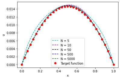
In this section, we verify numerically the convergence of the neural network PDE model for the exact neural network architecture and training method that is studied in our mathematical theory. As a simple example of the class of PDEs (1.2) that we studied in the mathematically theory, we consider the heat equation μ​ux​x−u=0\mu u_{xx}-u=0 in d=1d=1 and U=[0,1]U=[0,1]. The objective function (1.1) is constructed for a target function h⁡(x)=(1−x)​x5+x​(1−x)5h(x)=(1-x)x^{5}+x(1-x)^{5} and the orthonormal basis cos⁡(ℓ​π​x)\cos(\ell\pi x) with ℓ=0,…,9\ell=0,\ldots,9. The diffusion constant μ=110\mu=\frac{1}{10}. We use exactly the neural network architecture (1.4) for which our mathematical theory is proven with a choice of β=23\beta=\frac{2}{3} for the normalization factor. The parameters are trained with standard gradient descent (again as in our theoretical setting). The gradients are evaluated by solving the adjoint equation (1.3). An implicit solver is used for fast solutions of the forward neural network-equation (1.2) and its corresponding adjoint equation (1.3).

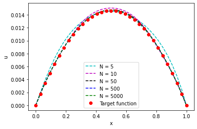
Results are presented below for different numbers of hidden units NN. For each value of NN, the neural network is randomly initialized with (A) i.i.d. Gaussian random variables for the (wi,bi)(w^{i},b^{i}) parameters and (B) i.i.d. uniform random variables for the cic^{i} parameters. This random initialization satisfies our Assumption 2.3. For each value of NN, the solution u⁡(x)u(x) to the heat equation (1.4) with the trained neural network f⁡(x,θ)f(x;\theta) is plotted in Figure 1. As the number of hidden units NN increases, the neural network PDE solution converges to the target function h⁡(x)h(x). We also evaluate the objective function (1.1) for the trained neural network PDE as the number of hidden units is increased. Table (1) reports the value of the objective function as the number of hidden units NN is increased; it quickly becomes very small for larger numbers of hidden units.
Refer to caption
Figure 1: Solutions to (1.2) in one spatial dimension as the number of hidden units NN increases. The target function h⁡(x)h(x) is also displayed for comparison.
N Objective Function
5 1.31×10−41.31\times 10^{-4}
10 9.49×10−59.49\times 10^{-5}
50 6.23×10−76.23\times 10^{-7}
250 2.49×10−102.49\times 10^{-10}
500 3.94×10−133.94\times 10^{-13}
Table 1: Value of the objective function (1.1) for the trained neural network PDE solution, in one spatial dimension, as the number of hidden units NN is increased.

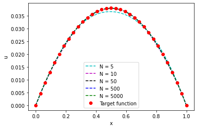
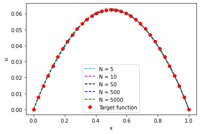
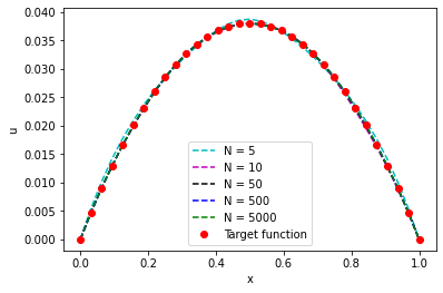
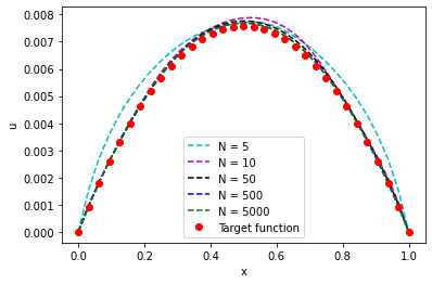
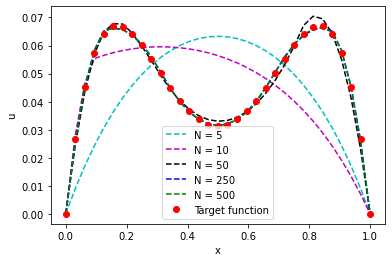
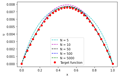
In addition, we also study the numerical convergence of the neural network PDE model for an example of (1.2) in two dimensions. Specifically, we consider the heat equation μ⁡(ux​x+uy​y)−u=0\mu(u_{xx}+u_{yy})-u=0 and U=[0,1]×[0,1]U=[0,1]\times[0,1] with μ=110\mu=\frac{1}{10}. The objective function (1.1) is constructed for a target function h⁡(x,y)=(x−x2)​(y−y2)h(x,y)=(x-x^{2})(y-y^{2}) and the orthonormal basis cos⁡(ℓx​π​x)×cos⁡(ℓy​π​y)\cos(\ell_{x}\pi x)\times\cos(\ell_{y}\pi y) with ℓx,ℓy=0,…,9\ell_{x},\ell_{y}=0,\ldots,9. The same neural network architecture, normalization factor, gradient descent algorithm, and parameter initialization are used as in the previous one-dimensional example. A 2D implicit solver is used for fast solutions of the forward neural network-equation (1.2) and its corresponding adjoint equation (1.3). The neural network and training algorithm match the framework studied in our mathematical theory. Results are presented below for different numbers of hidden units NN. For each value of NN, the neural network is randomly initialized, trained with gradient descent, and then the solution u⁡(x)u(x) to the heat equation (1.4) with the trained neural network f⁡(x,θ)f(x;\theta) is plotted in Figure 2. As the number of hidden units NN increases, the neural network PDE solution converges towards the target function h⁡(x)h(x). We also evaluate the objective function (1.1) for the trained neural network PDE as the number of hidden units is increased. Table (2) reports the value of the objective function as the number of hidden units NN is increased; it quickly becomes very small for larger numbers of hidden units.
Refer to caption
Refer to caption
Refer to caption
Refer to caption
Refer to caption
Refer to caption
Refer to caption
Refer to caption
Refer to caption
Figure 2: Solutions to (1.2) in two spatial dimensions as the number of hidden units NN increases. The target function h⁡(x)h(x) is also displayed for comparison. Solutions uN​(x,y)u^{N}(x,y) are plotted for different values of yy. In the top row: y=0.03125,0.0625,y=0.03125,0.0625, and 0.18750.1875. In the middle row: y=0.34375,0.5,y=0.34375,0.5, and 0.656250.65625. In the bottom row: y=0.8125,0.9375,y=0.8125,0.9375, and 0.968750.96875.
N Objective Function
5 7.03×10−87.03\times 10^{-8}
10 6.25×10−96.25\times 10^{-9}
50 1.25×10−91.25\times 10^{-9}
500 4.75×10−104.75\times 10^{-10}
5000 2.60×10−102.60\times 10^{-10}
Table 2: Value of the objective function (1.1) for the trained neural network PDE solution, in two spatial dimensions, as the number of hidden units NN is increased.

3.2 Example Application: RANS Turbulence Closures

In this section, we demonstrate that the approach can also be applied in practice to nonlinear equations. We use a neural network for closure of the RANS equations, which leads to a nonlinear differential equation model with neural network terms. The neural network RANS model is then trained, using the adjoint equations, to match target data generated from the fully resolved physics.

The incompressible Navier–Stokes equations

∂ui∂t+uj​∂ui∂xj\displaystyle\frac{\partial u_{i}}{\partial t}+u_{j}\frac{\partial u_{i}}{\partial x_{j}} =−1ρ​∂p∂xi+∂∂xj​[ν⁡(∂ui∂xj+∂uj∂xi)]\displaystyle=-\frac{1}{\rho}\frac{\partial p}{\partial x_{i}}+\frac{\partial}{\partial x_{j}}\left[\nu\left(\frac{\partial u_{i}}{\partial x_{j}}+\frac{\partial u_{j}}{\partial x_{i}}\right)\right] (3.1)
∂uj∂xj\displaystyle\frac{\partial u_{j}}{\partial x_{j}} =0\displaystyle=0 (3.2)

govern the evolution of a three-dimensional, unsteady velocity field ui​(xj,t)=(u,v,w)u_{i}(x_{j},t)=(u,v,w), where xj=(x,y,z)x_{j}=(x,y,z) are the Cartesian coordinates. Repeated indices imply summation. The mass density ρ\rho and kinematic viscosity ν\nu are constant, and the hydrodynamic pressure p⁡(xj,t)p(x_{j},t) is obtained from a Poisson equation [9] that discretely enforces the divergence-free constraint (3.2).

Direct Numerical Simulation (DNS) solves the Navier–Stokes equations with sufficient resolution such that the turbulence may be considered fully resolved. Doing so is prohibitively expensive for high Reynolds numbers or complicated geometries. The RANS approach averages along statistically homogeneous directions (potentially including time) and so reduces the dimensionality of (3.1) and (3.2) with concomitant cost reduction. However, the RANS equations contain unclosed terms that require modeling.

3.2.1 Turbulent Channel Flow

An application to turbulent channel flow is considered here. The flow is statistically homogeneous in the streamwise direction (xx), the spanwise direction (zz), and time (tt); hence the mean flow varies only in yy. The RANS-averaged velocity components are

u¯i​(y)=1Lx​Lz​(tf−t0)​∫t0tf∫0Lz∫0Lxui​(x,y,z,t)​𝑑x​𝑑z​𝑑t,\overline{u}_{i}(y)=\frac{1}{L_{x}L_{z}(t_{f}-t_{0})}\int_{t_{0}}^{t_{f}}\int_{0}^{L_{z}}\int_{0}^{L_{x}}u_{i}(x,y,z;t)\,\mathrm{d}x\,\mathrm{d}z\,\mathrm{d}t, (3.3)

where LxL_{x} and LzL_{z} are the extents of the computational domain in the xx- and zz-directions, respectively, and tf−t0t_{f}-t_{0} is the time interval over which averaging is performed. The cross-stream and spanwise mean velocity components are identically zero: v¯=w¯=0\overline{v}=\overline{w}=0. A schematic of the flow is shown in Figure 3.

Refer to caption
Figure 3: Schematic of the turbulent channel-flow configuration showing the domain extents and flow direction. Data is from instantaneous DNS of fully developed flow at Re=18×103\mathrm{Re}=18\times 10^{3} (Case D).

The three-dimensional, unsteady Navier–Stokes equations (3.1) and (3.2) are solved using DNS to provide high-resolution training and testing data. For turbulent channel flow, the characteristic length scale is the channel half-height δ=Ly/2\delta=L_{y}/2, and three characteristic velocity scales may be defined:

U¯\displaystyle\overline{U} ≡1δ∫0δu¯(y)dy(bulk velocity),\displaystyle\equiv\frac{1}{\delta}\int_{0}^{\delta}\overline{u}(y)\,\mathrm{d}y\qquad\text{(bulk velocity)},
U0\displaystyle U_{0} ≡u¯(y=0)(centerline velocity),\displaystyle\equiv\overline{u}(y=0)\qquad\quad\text{(centerline velocity)},
uτ\displaystyle u_{\tau} ≡τw/ρ(friction velocity),\displaystyle\equiv\sqrt{\tau_{w}/\rho}\qquad\quad\quad\text{(friction velocity)},

where τ⁡(y)=ρ​ν​(d​u¯/d​y)\tau(y)=\rho\nu(\mathrm{d}\overline{u}/\mathrm{d}y) is the mean shear stress and τw≡τ⁡(y=−δ)=−τ⁡(y=δ)\tau_{w}\equiv\tau(y=-\delta)=-\tau(y=\delta) is the wall shear stress. These define bulk, centerline, and friction Reynolds numbers

Re\displaystyle\mathrm{Re} ≡2​δ​U¯ν,\displaystyle\equiv\frac{2\delta\overline{U}}{\nu}, Re0\displaystyle\mathrm{Re}_{0} ≡δ​U0ν,\displaystyle\equiv\frac{\delta U_{0}}{\nu}, and Reτ\displaystyle\mathrm{Re}_{\tau} ≡uτ​δν=δδv,\displaystyle\equiv\frac{u_{\tau}\delta}{\nu}=\frac{\delta}{\delta_{v}},

respectively, where δv=ν/uτ\delta_{v}=\nu/u_{\tau} is a viscous length scale. Flow in the near-wall boundary layer is typically presented in terms of “wall units” y+=y/δvy^{+}=y/\delta_{v} and the corresponding normalized velocity u+=u¯/uτu^{+}=\overline{u}/u_{\tau}.

3.2.2 DNS Datasets

DNS datasets at Re={6,9,12,18,24}×103\mathrm{Re}=\{6,9,12,18,24\}\times 10^{3} were generated for training and testing. Table 3 lists the bulk, centerline, and friction Reynolds numbers for each, as well as the computed friction coefficient

Cf≡τw12​ρ​U¯2.C_{f}\equiv\frac{\tau_{w}}{\frac{1}{2}\rho\overline{U}^{2}}.

The friction coefficient for the Reτ=190\mathrm{Re}_{\tau}=190 case is in good agreement with that of the Reτ=180\mathrm{Re}_{\tau}=180 DNS of Kim, Moin, and Moser [40]. Table 3 also lists the status of each dataset as it was used for training or testing. The near-wall streamwise mean velocity, in wall units, is shown for each case in Figure 4, showing good agreement with the theoretical log-law, particularly for the higher-Reynolds-number cases.

Case Re\mathrm{Re} Re0\mathrm{Re}_{0} Reτ\mathrm{Re}_{\tau} CfC_{f} Train Test
A 6,001 3,380 190.0 8.02×10−38.02\times 10^{-3} ∙\bullet
B 9,000 5,232 270.3 7.22×10−37.22\times 10^{-3} ∙\bullet
C 12,000 6,800 345.3 6.62×10−36.62\times 10^{-3} ∙\bullet
D 18,000 10,191 495.0 6.05×10−36.05\times 10^{-3} ∙\bullet
E 24,000 13,440 638.2 5.66×10−35.66\times 10^{-3} ∙\bullet
Table 3: Reynolds numbers, friction coefficients, and train/test status for channel-flow DNS cases.
Figure 4: Mean velocity profiles in viscous units for DNS datasets listed in Table 3. The inner and log layers are indicated by dashed lines for reference.

The DNS solves the Navier–Stokes equations using second-order centered differences on a staggered mesh [23]. Time integration is by a fractional-step method [39] with a linearized trapezoid method in an alternating-direction implicit (ADI) framework for the viscous terms [25]. A fixed time-step size is used, with resulting CFL numbers about 0.35.

Uniform mesh spacings Δ​x=Lx/nx\Delta x=L_{x}/n_{x} and Δ​z=Lz/nz\Delta z=L_{z}/n_{z} are used in the xx- and zz-directions, respectively, where nxn_{x}, nyn_{y}, and nzn_{z} are the number of mesh cells in each direction. The mesh is stretched in the yy-direction, with discrete cell-face points given by a hyperbolic tangent function

yj=δtanh⁡[sy​(2​jny−1)]tanh⁡sy,j=0,1,…,ny,y_{j}=\delta\frac{\tanh\left[s_{y}\left(\frac{2j}{n_{y}}-1\right)\right]}{\tanh s_{y}},\qquad j=0,1,\dotsc,n_{y},

where sy=1.05s_{y}=1.05 is a stretching parameter. Grid resolutions, listed in Table 4, are sufficient to place the first cell midpoint 0.71≤Δ​yw+≤1.300.71\leq\Delta y_{w}^{+}\leq 1.30 from the wall with maximum centerline grid spacing 3.61≤Δ​y0+≤6.673.61\leq\Delta y_{0}^{+}\leq 6.67. Depending on the case, the xx- and zz-directions are discretized with resolutions between Δ​x+=Δ​x/δv=2.64\Delta x^{+}=\Delta x/\delta_{v}=2.64 and Δ​z+=Δ​z/δv=5.39\Delta z^{+}=\Delta z/\delta_{v}=5.39.

Case (Lx,Ly,Lz)/δ(L_{x},L_{y},L_{z})/\delta nx×ny×nzn_{x}\times n_{y}\times n_{z} Δ​yw+\Delta y^{+}_{w} Δ​y0+\Delta y^{+}_{0} Δ​x+\Delta x^{+} Δ​z+\Delta z^{+}
A 29×2×2429\times 2\times 24 1024×128×7681024\times 128\times 768 0.78 3.99 5.38 5.94
B 10×2×1010\times 2\times 10 1024×192×7681024\times 192\times 768 0.74 3.78 2.64 3.52
C 20×2×2020\times 2\times 20 1280×256×12801280\times 256\times 1280 0.71 3.61 5.39 5.39
D 10×2×1010\times 2\times 10 1280×256×12801280\times 256\times 1280 1.02 5.19 3.87 3.87
E 10×2×1010\times 2\times 10 1280×256×12801280\times 256\times 1280 1.30 6.67 4.99 4.99
Table 4: Domain sizes, grid sizes, and resolutions in wall units for turbulent channel-flow DNS cases.

3.2.3 Turbulent Channel-flow RANS

The momentum equation solved by RANS is obtained by applying (3.3) to (3.1) and letting tf→∞t_{f}\rightarrow\infty. For turbulent channel flow, it reduces to a steady, one-dimensional equation for the streamwise mean velocity component u¯​(y)\overline{u}(y),

0=−1ρ​d​p¯d​x+dd​y​(ν​d​u¯d​y−u′​v′¯),0=-\frac{1}{\rho}\frac{\mathrm{d}\overline{p}}{\mathrm{d}x}+\frac{\mathrm{d}}{\mathrm{d}y}\left(\nu\frac{\mathrm{d}\overline{u}}{\mathrm{d}y}-\overline{u^{\prime}v^{\prime}}\right), (3.4)

which is essentially the heat equation with a streamwise pressure-gradient forcing term dp¯/dx=−τw/δ\mathrm{d}\overline{p}/\mathrm{d}x=-\tau_{w}/\delta, which is adjusted to maintain constant U¯=1\overline{U}=1. Note that d​p¯/d​x\mathrm{d}\overline{p}/\mathrm{d}x is uniform in yy. The term u′​v′¯\overline{u^{\prime}v^{\prime}} (the Reynolds stress) represents the action of the velocity fluctuations ui′=ui−u¯iu_{i}^{\prime}=u_{i}-\overline{u}_{i} on the mean flow and is unclosed. A standard closure model used for comparison is summarized in Sec. 3.2.4, and the neural network model to be tested is described in Sec. 3.2.5.

3.2.4 The kk-ϵ\epsilon Model

The eddy-viscosity (Boussinesq) hypothesis enables one to relate the Reynolds stress to the mean velocity gradients and so close (3.4). For turbulent channel flow, the eddy-viscosity hypothesis is stated

u′​v′¯=−νt​d​u¯d​y,\overline{u^{\prime}v^{\prime}}=-\nu_{t}\frac{\mathrm{d}\overline{u}}{\mathrm{d}y}, (3.5)

where νt\nu_{t} is the eddy viscosity to be computed. Applying (3.5) to (3.4), the RANS equation is

0=−1ρ​∂p¯∂x+dd​y​[(ν+νt)​d​u¯d​y],0=-\frac{1}{\rho}\frac{\partial\overline{p}}{\partial x}+\frac{\mathrm{d}}{\mathrm{d}y}\left[(\nu+\nu_{t})\frac{\mathrm{d}\overline{u}}{\mathrm{d}y}\right], (3.6)

which is closed.

The eddy viscosity may be obtained in many ways. It is likely that the most common approach for engineering applications is the standard kk-ϵ\epsilon model [35, 45], which is a “two-equation” model in that it requires the solution of two additional PDEs. It computes νt\nu_{t} from

νt=Cμ​k2ϵ,\nu_{t}=C_{\mu}\frac{k^{2}}{\epsilon}, (3.7)

where k≡12​ui′​ui′¯k\equiv\frac{1}{2}\overline{u_{i}^{\prime}u_{i}^{\prime}} is the turbulent kinetic energy (TKE), ϵ\epsilon is the TKE dissipation rate, and CμC_{\mu} is a model parameter. The TKE and its dissipation rate may be computed from DNS and experimental data but are unclosed in RANS. Instead, the kk-ϵ\epsilon model obtains them from PDEs with modeled terms, which for channel flow reduce to

0\displaystyle 0 =dd​y​(ν+νtσk​d​kd​y)+νt​(d​u¯d​y)2−ϵ,\displaystyle=\frac{\mathrm{d}}{\mathrm{d}y}\left(\frac{\nu+\nu_{t}}{\sigma_{k}}\frac{\mathrm{d}k}{\mathrm{d}y}\right)+\nu_{t}\left(\frac{\mathrm{d}\overline{u}}{\mathrm{d}y}\right)^{2}-\epsilon,
0\displaystyle 0 =dd​y​(ν+νtσϵ​d​ϵd​y)+C1​ϵ​Cμ​k​(d​u¯d​y)2−C2​ϵ​ϵ2k.\displaystyle=\frac{\mathrm{d}}{\mathrm{d}y}\left(\frac{\nu+\nu_{t}}{\sigma_{\epsilon}}\frac{\mathrm{d}\epsilon}{\mathrm{d}y}\right)+C_{1\epsilon}C_{\mu}k\left(\frac{\mathrm{d}\overline{u}}{\mathrm{d}y}\right)^{2}-C_{2\epsilon}\frac{\epsilon^{2}}{k}. (3.8)

Typical values for the constants are [45]:

Cμ\displaystyle C_{\mu} =0.09,\displaystyle=0.09, σk\displaystyle\sigma_{k} =1.00,\displaystyle=1.00, σϵ\displaystyle\sigma_{\epsilon} =1.30,\displaystyle=1.30, C1​ϵ\displaystyle C_{1\epsilon} =1.44,…. and\displaystyle=1.44,\textrm{\phantom{....} and} C2​ϵ\displaystyle C_{2\epsilon} =1.92.\displaystyle=1.92.

3.2.5 Neural Network Closure

Our neural network RANS model augments the eddy-viscosity model (3.5) by

u′​v′¯=−νt​d​u¯d​y+f1​(y,k,ϵ,d​u¯d​y,θ)+CRRe​f2​(y,k,ϵ,d​u¯d​y,θ),\overline{u^{\prime}v^{\prime}}=-\nu_{t}\frac{\mathrm{d}\overline{u}}{\mathrm{d}y}+f_{1}\left(y,k,\epsilon,\frac{\mathrm{d}\overline{u}}{\mathrm{d}y},\theta\right)+\frac{C_{R}}{\mathrm{Re}}f_{2}\left(y,k,\epsilon,\frac{\mathrm{d}\overline{u}}{\mathrm{d}y},\theta\right), (3.9)

where f⁡(⋅,θ)f(\cdot,\theta) is a neural network with a vector output, fi​(⋅,θ)f_{i}(\cdot,\theta) is the ii-th output of the neural network, and θ\theta are its parameters. The constant CR=6,001C_{R}=6,001 is the lowest Reynolds number in the training dataset. The input variables for the neural network are (y,k,ϵ,d​u¯/d​y)(y,k,\epsilon,\mathrm{d}\overline{u}/\mathrm{d}y).

The RANS equation with the eddy-viscosity model and the neural network is

0=−1ρ​d​p¯d​x+dd​y​[(ν+νt)​d​u¯d​y−f1​(y,k,ϵ,d​u¯d​y,θ)−CRRe​f2​(y,k,ϵ,d​u¯d​y,θ)],0=-\frac{1}{\rho}\frac{\mathrm{d}\overline{p}}{\mathrm{d}x}+\frac{\mathrm{d}}{\mathrm{d}y}\left[(\nu+\nu_{t})\frac{\mathrm{d}\overline{u}}{\mathrm{d}y}-f_{1}\left(y,k,\epsilon,\frac{\mathrm{d}\overline{u}}{\mathrm{d}y},\theta\right)-\frac{C_{R}}{\mathrm{Re}}f_{2}\left(y,k,\epsilon,\frac{\mathrm{d}\overline{u}}{\mathrm{d}y},\theta\right)\right], (3.10)

with νt\nu_{t}, kk, and ϵ\epsilon obtained as above.

The optimization of the PDE model (3.10) is a nonlinear version of our mathematical framework (1.2). The objective function for the model is the mean-squared error for the velocity profile (which can be thought of as a strong formulation of the objective function (1.1)):

J⁡(θ)=12​∫−δδ(h⁡(y)−u¯​(y))2​𝑑y,J(\theta)=\frac{1}{2}\int_{-\delta}^{\delta}\bigg(h(y)-\overline{u}(y)\bigg)^{2}dy, (3.11)

where the target profile h⁡(y)h(y) is the averaged DNS data, and u¯\overline{u} is the solution to (3.10). The operator AA from (1.2) has, in this case, become a nonlinear operator AA acting on (u¯,k,ϵ)(\overline{u},k,\epsilon) and corresponding to the right-hand side of the equations (3.10) and (3.8). Specifically,

A​(u¯kϵ)\displaystyle A\begin{pmatrix}\overline{u}\\ k\\ \epsilon\end{pmatrix} =\displaystyle= (−1ρ​d​p¯d​x+dd​y​[(ν+νt)​d​u¯d​y]dd​y​(ν+νtσk​d​kd​y)+νt​(d​u¯d​y)2−ϵdd​y​(ν+νtσϵ​d​ϵd​y)+C1​ϵ​Cμ​k​(d​u¯d​y)2−C2​ϵ​ϵ2k),\displaystyle\begin{pmatrix}-\frac{1}{\rho}\frac{\mathrm{d}\overline{p}}{\mathrm{d}x}+\frac{\mathrm{d}}{\mathrm{d}y}[(\nu+\nu_{t})\frac{\mathrm{d}\overline{u}}{\mathrm{d}y}]\\ \frac{\mathrm{d}}{\mathrm{d}y}\left(\frac{\nu+\nu_{t}}{\sigma_{k}}\frac{\mathrm{d}k}{\mathrm{d}y}\right)+\nu_{t}(\frac{\mathrm{d}\overline{u}}{\mathrm{d}y})^{2}-\epsilon\\ \frac{\mathrm{d}}{\mathrm{d}y}\left(\frac{\nu+\nu_{t}}{\sigma_{\epsilon}}\frac{\mathrm{d}\epsilon}{\mathrm{d}y}\right)+C_{1\epsilon}C_{\mu}k(\frac{\mathrm{d}\overline{u}}{\mathrm{d}y})^{2}-C_{2\epsilon}\frac{\epsilon^{2}}{k}\end{pmatrix},

where we recall that the forcing term dp¯/dx=−τw/δ\mathrm{d}\overline{p}/\mathrm{d}x=-\tau_{w}/\delta plus an adaptive term to enforce U¯≈1\overline{U}\approx 1, where τw=ρ​ν​(d​u¯/d​y)y=−δ\tau_{w}=\rho\nu(\mathrm{d}\overline{u}/\mathrm{d}y)_{y=-\delta} is the wall shear stress defined in Subsection 3.2.1.

3.2.6 Numerical Results

The RANS equations are discretized using second-order centered differences on a staggered mesh. The solution u¯\overline{u} and its adjoint are computed at the yy-faces, and the model variables kk and ϵ\epsilon are computed at cell centers. A coarse grid of ny=32n_{y}=32 mesh points is used for all Reynolds numbers. The grid is nonuniform and is generated by the transformation

y~=sin⁡(η​π​y^/2)sin⁡(η​π/2),\tilde{y}=\frac{\sin(\eta\pi\hat{y}/2)}{\sin(\eta\pi/2)}, (3.12)

where y^∈[−δ,δ]\hat{y}\in[-\delta,\delta] is a uniform grid and η=0.995\eta=0.995. The system is solved using a pseudo-time-stepping scheme, in which the velocity solution is relaxed from an initially parabolic (laminar) profile using the fourth-order Runge–Kutta method until the solution has converged. Thus, although the RANS equations for channel flow satisfy a system of nonlinear differential equations, their solution is obtained by solving a time-dependent PDE.

We train the neural network-augmented closure model (3.9) on the DNS-evaluated mean velocity for Re={6,12,18}×103\mathrm{Re}=\{6,12,18\}\times 10^{3}. The adjoint of (3.10) is constructed using automatic differentiation as implemented by the Pytorch library [64]. 100 relaxation steps are taken per optimization iteration. Efficient, scalable training is performed using MPI parallelization and GPU offloading. The learning rate is decayed during training according to a piecewise constant learning rate schedule. Quadrature on the finite difference mesh is used to approximate the objective function.

The neural network architecture is similar to that used for [49] and [62]. Exponential linear units (ELUs) and sigmoids are used for the activation functions. Note that ELUs violate the assumption on boundedness of the activation function under which our theoretical results hold. Nevertheless, this example demonstrates that the mathematical results of this paper may indeed be true under less stringent assumptions. The neural network architecture is:

H(1)​(z,θ)\displaystyle H^{(1)}(z;\theta) =\displaystyle= ELU​(W(1)​z+b(1)),\displaystyle\textrm{ELU}(W^{(1)}z+b^{(1)}),
H(2)​(z,θ)\displaystyle H^{(2)}(z;\theta) =\displaystyle= ELU​(W(2)​H(1)​(z,θ)+b(2)),\displaystyle\textrm{ELU}(W^{(2)}H^{(1)}(z;\theta)+b^{(2)}),
G⁡(z,θ)\displaystyle G(z;\theta) =\displaystyle= σ⁡(W(3)​z+b(3)),\displaystyle\sigma(W^{(3)}z+b^{(3)}),
U⁡(z,θ)\displaystyle U(z;\theta) =\displaystyle= G⁡(z,θ)⊙H(2)​(z,θ),\displaystyle G(z;\theta)\odot H^{(2)}(z;\theta),
f⁡(z,θ)\displaystyle f(z;\theta) =\displaystyle= W(4)​U​(z,θ)+b(4),\displaystyle W^{(4)}U(z;\theta)+b^{(4)}, (3.13)

where the parameters θ={W(1),b(1),W(2),b(2),W(3),b(4)}\theta=\{W^{(1)},b^{(1)},W^{(2)},b^{(2)},W^{(3)},b^{(4)}\}, ⊙\odot denotes the element-wise product, ELU​(⋅)\textrm{ELU}(\cdot) is an element-wise ELU activation function, and σ⁡(⋅)\sigma(\cdot) is an element-wise sigmoid activation function.

Once trained, the neural network-augmented model (3.9) is tested out-of-sample at Re={9,24}×103\mathrm{Re}=\{9,24\}\times 10^{3}. We observed that if the model was optimized for a very large number of iterations, instability could occur (presumably due to the equations becoming very stiff near the walls) or it could overfit on the test cases. The results presented are for a model trained with a moderately large number of optimization iterations which produces both good performances on the training cases as well as the test cases. The results provide a useful numerical example of this paper’s optimization method applied to nonlinear equations, but the challenges with overfitting on out-of-sample Reynolds numbers suggest that perhaps a PDE model with more physics (such as large-eddy simulation) should be combined with a neural network closure model instead of using RANS. The training mean-squared error is ∼1.8×10⁻³\sim 1.8\times 10^{-3}. Figures 5 and 6 compare the mean velocity in mean-flow and wall units, respectively, for the DNS, RANS with the standard kk-ϵ\epsilon model, and RANS with the neural network-augmented model. The neural network model improves the accuracy of the kk-ϵ\epsilon model. In particular, the near-wall prediction (Figure 6) is improved by the neural network but still does not exactly match the DNS, as might be anticipated for the coarse grid.

Figure 5: Mean velocity profiles obtained from spatio-temporally averaged DNS, RANS using the standard kk-ϵ\epsilon model, and RANS using the neural network-augmented model. DNS were computed using the meshes in Table 4; points indicate the cell-face locations used for the RANS calculations. Left: Re=9×10³\mathrm{Re}=9\times 10^{3}; right: Re=24×103\mathrm{Re}=24\times 10^{3}. The neural network model was trained on Re={6,12,18}×103\mathrm{Re}=\{6,12,18\}\times 10^{3}.
Figure 6: Mean velocity profiles in viscous units for out-of-sample testing cases: Re={9,24}×103\mathrm{Re}=\{9,24\}\times 10^{3}. Solid lines: DNS; dotted lines: RANS with the kk-ϵ\epsilon model; dashed lines: RANS with the neural network-augmented model. The log-law is indicated by dashed lines for reference. The friction velocity used to normalize each Reτ\mathrm{Re}_{\tau} was computed from DNS. The solid lines for the two DNS datasets nearly overlap.

4 A-priori preliminary bounds

Let us start by obtaining certain crucial a-priori bounds. The gradient of the objective function (1.1) can be evaluated using the solution u^\hat{u} to the adjoint PDE (1.3). Indeed, this is the statement of Lemma 4.1 below.

Lemma 4.1.

Let Assumptions 2.1, 2.2 hold. Then,

∇θJ​(θ)=∫Uu^​(x,f)​∇θf​(x,θ)​𝑑x\displaystyle\nabla_{\theta}J(\theta)=\int_{U}\hat{u}(x;f)\nabla_{\theta}f(x,\theta)dx (4.1)
Proof of Lemma 4.1.

We start by defining u~=∇θu\tilde{u}=\nabla_{\theta}u. If we differentiate (1.2) we obtain

A​u~​(x)\displaystyle A\tilde{u}(x) =∇θf​(x,θ),x∈U\displaystyle=\nabla_{\theta}f(x,\theta),\quad x\in U
u~​(x)\displaystyle\tilde{u}(x) =0,x∈∂U\displaystyle=0,\quad x\in\partial U

Integration by parts gives

(u^,A​u~)\displaystyle(\hat{u},A\tilde{u}) =\displaystyle= (A†​u^,u~).\displaystyle(A^{\dagger}\hat{u},\tilde{u}).

Using now (1.2) and (1.3) for the left and right hand side we obtain

(⟨u,m⟩−⟨h,m⟩)⊤​(u~,m)\displaystyle(\left\langle u,m\right\rangle-\left\langle h,m\right\rangle)^{\top}(\tilde{u},m) =\displaystyle= (u^,∇θf​(θ)).\displaystyle(\hat{u},\nabla_{\theta}f(\theta)).

Due to (1.1), we finally obtain

∇θJ​(θ)\displaystyle\nabla_{\theta}J(\theta) =\displaystyle= ∇θ[12​(⟨u,m⟩−⟨h,m⟩)⊤​(⟨u,m⟩−⟨h,m⟩)]\displaystyle\nabla_{\theta}\bigg[\frac{1}{2}(\left\langle u,m\right\rangle-\left\langle h,m\right\rangle)^{\top}(\left\langle u,m\right\rangle-\left\langle h,m\right\rangle)\bigg] (4.2)
=\displaystyle= (⟨u,m⟩−⟨h,m⟩)⊤​⟨u~,m⟩\displaystyle(\left\langle u,m\right\rangle-\left\langle h,m\right\rangle)^{\top}\left\langle\tilde{u},m\right\rangle
=\displaystyle= (u^,∇θf​(θ)),\displaystyle(\hat{u},\nabla_{\theta}f(\theta)),\

which concludes the proof of the lemma. ∎

Lemma 4.1 shows that the gradient descent update can be written as follows:

θ˙ti\displaystyle\dot{\theta}_{t}^{i} =\displaystyle= −αN​∇θtiJ​(θt)\displaystyle-\alpha^{N}\nabla_{\theta^{i}_{t}}J(\theta_{t}) (4.3)
=\displaystyle= −αk,N​(u^N​(t,x),∇θtif​(x,θt))L2​(U),\displaystyle-\alpha^{k,N}\left(\hat{u}^{N}(t,x),\nabla_{\theta^{i}_{t}}f(x,\theta_{t})\right)_{L^{2}(U)},

It can be proven that the gradient descent updates are uniformly bounded with respect to t,Nt,N for t≤Tt\leq T for a given T<∞T<\infty.

Lemma 4.2.

Let T<∞T<\infty be given and Assumptions 2.1-2.3 hold. There exists a finite constant C<∞C<\infty, depending on TT and on the operator AA, such that for all i∈ℕi\in\mathbb{N} and all t∈[0,T]t\in[0,T],

supi∈{1,⋯,N},N∈ℕ,t∈[0,T]|cti|\displaystyle\sup_{i\in\{1,\cdots,N\},N\in\mathbb{N},t\in[0,T]}|c_{t}^{i}| ≤C<∞,\displaystyle\leq C<\infty,
supi∈{1,⋯,N},N∈ℕ,t∈[0,T]𝔼⁡(‖wti‖+|ηti|)\displaystyle\sup_{i\in\{1,\cdots,N\},N\in\mathbb{N},t\in[0,T]}\mathbb{E}\left(\left\lVert w_{t}^{i}\right\rVert+|\eta_{t}^{i}|\right) ≤C<∞.\displaystyle\leq C<\infty.
Proof of Lemma 4.2.

We start with a bound on ‖u^N​(t)‖H01​(U)\left\lVert\hat{u}^{N}(t)\right\rVert_{H^{1}_{0}(U)}. Using standard elliptic estimates based on the implied coercivity by Assumption 2.1 and the Cauchy–Schwarz inequality, we obtain that there is a constant C<∞C<\infty such that

‖u^N​(t)‖H01​(U)2\displaystyle\left\lVert\hat{u}^{N}(t)\right\rVert^{2}_{H^{1}_{0}(U)} ≤‖(⟨uN​(t),m⟩−⟨h,m⟩)⊤​m‖L2​(U)2\displaystyle\leq\left\lVert(\left\langle u^{N}(t),m\right\rangle-\left\langle h,m\right\rangle)^{\top}m\right\rVert_{L^{2}(U)}^{2}
≤C​‖⟨uN​(t),m⟩−⟨h,m⟩‖22​‖m‖L2​(U)2\displaystyle\leq C\left\lVert\left\langle u^{N}(t),m\right\rangle-\left\langle h,m\right\rangle\right\rVert_{2}^{2}\left\lVert m\right\rVert_{L^{2}(U)}^{2}
≤C⁡[‖uN​(t)‖L2​(U)2+‖h‖L2​(U)2]\displaystyle\leq C\left[\left\lVert u^{N}(t)\right\rVert^{2}_{L^{2}(U)}+\left\lVert h\right\rVert^{2}_{L^{2}(U)}\right]
≤C⁡[‖uN​(t)‖H01​(U)2+‖h‖L2​(U)2]\displaystyle\leq C\left[\left\lVert u^{N}(t)\right\rVert^{2}_{H^{1}_{0}(U)}+\left\lVert h\right\rVert^{2}_{L^{2}(U)}\right]
≤C⁡[‖gtN‖L2​(U)2+‖h‖L2​(U)2]\displaystyle\leq C\left[\left\lVert g^{N}_{t}\right\rVert^{2}_{L^{2}(U)}+\left\lVert h\right\rVert^{2}_{L^{2}(U)}\right]
≤C⁡[1N2​β​∫UN​∑i=1N|cti|2​|σ⁡(wti​x+ηti)|2​𝑑x+‖h‖L2​(U)2]\displaystyle\leq C\left[\frac{1}{N^{2\beta}}\int_{U}N\sum_{i=1}^{N}|c^{i}_{t}|^{2}|\sigma(w^{i}_{t}x+\eta_{t}^{i})|^{2}dx+\left\lVert h\right\rVert^{2}_{L^{2}(U)}\right]
≤C⁡[1N2​β−2​1N​∑i=1N|cti|2+‖h‖L2​(U)2],\displaystyle\leq C\left[\frac{1}{N^{2\beta-2}}\frac{1}{N}\sum_{i=1}^{N}|c^{i}_{t}|^{2}+\left\lVert h\right\rVert^{2}_{L^{2}(U)}\right],

where in the last line we used the uniform boundedness of σ\sigma. Let us set κtN=1N​∑i=1N|cti|2\kappa_{t}^{N}=\displaystyle\frac{1}{N}\sum_{i=1}^{N}|c^{i}_{t}|^{2}. The last display gives us

‖u^N​(t)‖H01​(U)2\displaystyle\left\lVert\hat{u}^{N}(t)\right\rVert^{2}_{H^{1}_{0}(U)} ≤C⁡[1N2​β−2​κtN+‖h‖L2​(U)2].\displaystyle\leq C\left[\frac{1}{N^{2\beta-2}}\kappa_{t}^{N}+\left\lVert h\right\rVert^{2}_{L^{2}(U)}\right].

Next, we calculate

cti\displaystyle c^{i}_{t} =c0i−αN1−β​∫0t∫Uu^N​(s,x)​σ​(wsi​x+ηsi)​𝑑x​𝑑s,\displaystyle=c^{i}_{0}-\frac{\alpha}{N^{1-\beta}}\int_{0}^{t}\int_{U}\hat{u}^{N}(s,x)\sigma(w^{i}_{s}x+\eta_{s}^{i})dxds,

which then implies due to the assumed uniform boundedness of σ\sigma that

|cti|\displaystyle|c^{i}_{t}| ≤|c0i|+α​‖σ‖N1−β​∫0t∫U|u^N​(s,x)|​𝑑x​𝑑s.\displaystyle\leq|c^{i}_{0}|+\frac{\alpha\left\lVert\sigma\right\rVert}{N^{1-\beta}}\int_{0}^{t}\int_{U}|\hat{u}^{N}(s,x)|dxds.

This then gives

|cti|2\displaystyle|c^{i}_{t}|^{2} ≤2​|c0i|2+CN2​(1−β)​t​∫0t‖u^N​(s)‖L2​(U)2​𝑑s\displaystyle\leq 2|c^{i}_{0}|^{2}+\frac{C}{N^{2(1-\beta)}}t\int_{0}^{t}\left\lVert\hat{u}^{N}(s)\right\rVert^{2}_{L^{2}(U)}ds
≤2​|c0i|2+CN2​(1−β)​t​∫0t[1N2​β−2​κsN+‖h‖L2​(U)2]​𝑑s\displaystyle\leq 2|c^{i}_{0}|^{2}+\frac{C}{N^{2(1-\beta)}}t\int_{0}^{t}\left[\frac{1}{N^{2\beta-2}}\kappa_{s}^{N}+\left\lVert h\right\rVert^{2}_{L^{2}(U)}\right]ds (4.4)

Normalizing by NN and summing up over all i=1,⋯,Ni=1,\cdots,N gives

κtN\displaystyle\kappa_{t}^{N} ≤2​κ0N+CN2​(1−β)​t​∫0t[1N2​β−2​κsN+‖h‖L2​(U)2]​𝑑s\displaystyle\leq 2\kappa_{0}^{N}+\frac{C}{N^{2(1-\beta)}}t\int_{0}^{t}\left[\frac{1}{N^{2\beta-2}}\kappa_{s}^{N}+\left\lVert h\right\rVert^{2}_{L^{2}(U)}\right]ds
≤2​κ0N+C​t​∫0tκsN​𝑑s+C​t2N2−2​β​‖h‖L2​(U)2\displaystyle\leq 2\kappa_{0}^{N}+Ct\int_{0}^{t}\kappa_{s}^{N}ds+\frac{Ct^{2}}{N^{2-2\beta}}\left\lVert h\right\rVert^{2}_{L^{2}(U)}

Since c0ic^{i}_{0} take values in a compact set, there exists a constant C<∞C<\infty such that κ0N≤C\kappa_{0}^{N}\leq C. Hence, using the discrete Gronwall lemma we get that there is a constant (still denoted by) CC that may depend on TT, but not on NN, such that

supt∈[0,T]κtN\displaystyle\sup_{t\in[0,T]}\kappa_{t}^{N} ≤C.\displaystyle\leq C.

Combining the latter with (4.4) gives for some unimportant constant C<∞C<\infty

|cti|2\displaystyle|c^{i}_{t}|^{2} ≤2​|c0i|2+C+CN2​(1−β)​‖h‖L2​(U)2,\displaystyle\leq 2|c^{i}_{0}|^{2}+C+\frac{C}{N^{2(1-\beta)}}\left\lVert h\right\rVert^{2}_{L^{2}(U)}, (4.5)

from which the result follows, concluding the bound for |cti||c^{i}_{t}|. Now, we turn to the bound for ‖wti‖\left\lVert w^{i}_{t}\right\rVert. Using the uniform bound for |Cki||C^{i}_{k}| and Assumptions 2.1-2.3 on the boundedness of the domain UU and on σ′\sigma^{\prime} we get

‖wti‖\displaystyle\left\lVert w^{i}_{t}\right\rVert ≤‖w0i‖+αN1−β​∫0t∫U|u^N​(s,x)||csi​|σ′​(wsi​x+ηsi)​x|​𝑑x​𝑑s\displaystyle\leq\left\lVert w^{i}_{0}\right\rVert+\frac{\alpha}{N^{1-\beta}}\int_{0}^{t}\int_{U}|\hat{u}^{N}(s,x)||c^{i}_{s}|\sigma^{\prime}(w^{i}_{s}x+\eta_{s}^{i})x|dxds
≤‖w0i‖+CN1−β​∫0t‖u^N​(s)‖L1​(U)​|csi|​𝑑s\displaystyle\leq\left\lVert w^{i}_{0}\right\rVert+\frac{C}{N^{1-\beta}}\int_{0}^{t}\left\lVert\hat{u}^{N}(s)\right\rVert_{L^{1}(U)}|c^{i}_{s}|ds
≤‖w0i‖+CN1−β​∫0t[1Nβ−1+‖h‖L2​(U)]​𝑑s\displaystyle\leq\left\lVert w^{i}_{0}\right\rVert+\frac{C}{N^{1-\beta}}\int_{0}^{t}\left[\frac{1}{N^{\beta-1}}+\left\lVert h\right\rVert_{L^{2}(U)}\right]ds
≤‖w0i‖+C⁡[1+1N1−β],\displaystyle\leq\left\lVert w^{i}_{0}\right\rVert+C\left[1+\frac{1}{N^{1-\beta}}\right],

for a constant C<∞C<\infty that may change from line to line. From this we directly obtain that

supi∈{1,⋯,N},N∈ℕ,t∈[0,T]𝔼⁡‖wti‖≤C<∞.\displaystyle\sup_{i\in\{1,\cdots,N\},N\in\mathbb{N},t\in[0,T]}\mathbb{E}\left\lVert w^{i}_{t}\right\rVert\leq C<\infty.

The proof for the bound of supi∈{1,⋯,N},N∈ℕ,t∈[0,T]𝔼​|ηti|\sup_{i\in\{1,\cdots,N\},N\in\mathbb{N},t\in[0,T]}\mathbb{E}|\eta^{i}_{t}| is exactly the same as the uniform bound for 𝔼​‖wti‖\mathbb{E}\left\lVert w^{i}_{t}\right\rVert, concluding the proof of the lemma. ∎

Next, in Lemma 4.3, we show an important a-priori bound relating the neural network output gNg^{N} with the solution to the adjoint equation u^N\hat{u}^{N}.

Lemma 4.3.

For every T<∞T<\infty, we have that there is some constant C<∞C<\infty (independent of N) such that for all t∈[0,T]t\in[0,T] such that

maxs∈[0,t]⁡𝔼⁡[‖gsN‖L2​(U)2]\displaystyle\max_{s\in[0,t]}\mathbb{E}\bigg[\left\lVert g_{s}^{N}\right\rVert^{2}_{L^{2}(U)}\bigg] ≤C⁡(1+∫0tmaxτ∈[0,s]⁡𝔼⁡[‖u^N​(τ)‖L2​(U)2]​𝑑s).\displaystyle\leq C\bigg(1+\int_{0}^{t}\max_{\tau\in[0,s]}\mathbb{E}\bigg[\left\lVert\hat{u}^{N}(\tau)\right\rVert^{2}_{L^{2}(U)}\bigg]ds\bigg).
Proof of Lemma 4.3.

Starting with gtN​(x)=1Nβ​∑i=1Ncti​σ​(wti​x+ηti)g_{t}^{N}(x)=\displaystyle\frac{1}{N^{\beta}}\sum_{i=1}^{N}c^{i}_{t}\sigma(w^{i}_{t}x+\eta^{i}_{t}) and differentiating using (2.3) we obtain

g˙tN​(x)\displaystyle\dot{g}_{t}^{N}(x) =1Nβ​∑i=1N[c˙ti​σ​(wti​x+ηti)+cti​σ′​(wti​x+ηti)​(w˙ti​x+η˙ti)]\displaystyle=\frac{1}{N^{\beta}}\sum_{i=1}^{N}\left[\dot{c}^{i}_{t}\sigma(w^{i}_{t}x+\eta^{i}_{t})+c^{i}_{t}\sigma^{\prime}(w^{i}_{t}x+\eta^{i}_{t})(\dot{w}^{i}_{t}x+\dot{\eta}^{i}_{t})\right]
=−αN∑i=1N[∫Uu^N(t,x′)(σ(wtix+ηti)σ(wtix′+ηti)+|cti|2σ′(wtix+ηti)σ′(wtix′+ηti)(xx′+1))dx′]\displaystyle=-\frac{\alpha}{N}\sum_{i=1}^{N}\left[\int_{U}\hat{u}^{N}(t,x^{\prime})\left(\sigma(w^{i}_{t}x+\eta^{i}_{t})\sigma(w^{i}_{t}x^{\prime}+\eta^{i}_{t})+|c^{i}_{t}|^{2}\sigma^{\prime}(w^{i}_{t}x+\eta^{i}_{t})\sigma^{\prime}(w^{i}_{t}x^{\prime}+\eta^{i}_{t})(xx^{\prime}+1)\right)dx^{\prime}\right]

Recalling now the empirical measure μtN=1N​∑i=1Nδcti,wti,ηti\mu^{N}_{t}=\displaystyle\frac{1}{N}\sum_{i=1}^{N}\delta_{c^{i}_{t},w^{i}_{t},\eta^{i}_{t}} and the definition of B⁡(x,x′,μ)B(x,x^{\prime};\mu) by (2.5) we obtain the representation

g˙tN​(x)\displaystyle\dot{g}_{t}^{N}(x) =−∫Uu^N(t,x′)B(x,x′;μsN)dx′\displaystyle=-\int_{U}\hat{u}^{N}(t,x^{\prime})B(x,x^{\prime};\mu^{N}_{s})dx^{\prime} (4.6)

The latter implies that

‖gtN‖L2​(U)2\displaystyle\left\lVert g^{N}_{t}\right\rVert^{2}_{L^{2}(U)} ≤‖g0N‖L2​(U)2+∫U(∫0t∫Uu^N​(s,x′)​B​(x,x′,μsN)​d​x′​𝑑s)2​𝑑x\displaystyle\leq\left\lVert g^{N}_{0}\right\rVert^{2}_{L^{2}(U)}+\int_{U}\left(\int_{0}^{t}\int_{U}\hat{u}^{N}(s,x^{\prime})B(x,x^{\prime};\mu^{N}_{s})dx^{\prime}ds\right)^{2}dx

Notice now that for an appropriate constant CC (independent of NN) that may change from line to line

|B⁡(x,x′,μsN)|\displaystyle|B(x,x^{\prime};\mu^{N}_{s})| ≤α​1N​∑i=1N|σ⁡(wsi​x+ηsi)​σ​(wsi​x′+ηsi)+|csi|2​σ′​(wsi​x+ηsi)​σ′​(wsi​x′+ηsi)​(x​x′+1)|\displaystyle\leq\alpha\frac{1}{N}\sum_{i=1}^{N}\left|\sigma(w^{i}_{s}x+\eta^{i}_{s})\sigma(w^{i}_{s}x^{\prime}+\eta^{i}_{s})+|c^{i}_{s}|^{2}\sigma^{\prime}(w^{i}_{s}x+\eta^{i}_{s})\sigma^{\prime}(w^{i}_{s}x^{\prime}+\eta^{i}_{s})(xx^{\prime}+1)\right|
≤C⁡[1+1N​∑i=1N|csi|2]\displaystyle\leq C\left[1+\frac{1}{N}\sum_{i=1}^{N}|c^{i}_{s}|^{2}\right]
≤C,\displaystyle\leq C,

due to the boudnedness of σ,σ′,U\sigma,\sigma^{\prime},U and by Lemma 4.2. Thus, we have for an appropriate constant CC that

‖gtN‖L2​(U)2\displaystyle\left\lVert g^{N}_{t}\right\rVert^{2}_{L^{2}(U)} ≤‖g0N‖L2​(U)2+C​∫U(∫0t∫U|u^N​(s,x′)|​d​x′​𝑑s)2​𝑑x\displaystyle\leq\left\lVert g^{N}_{0}\right\rVert^{2}_{L^{2}(U)}+C\int_{U}\left(\int_{0}^{t}\int_{U}|\hat{u}^{N}(s,x^{\prime})|dx^{\prime}ds\right)^{2}dx
≤‖g0N‖L2​(U)2+C​(∫0t‖u^N​(s)‖L2​(U)​𝑑s)2\displaystyle\leq\left\lVert g^{N}_{0}\right\rVert^{2}_{L^{2}(U)}+C\left(\int_{0}^{t}\left\lVert\hat{u}^{N}(s)\right\rVert_{L^{2}(U)}ds\right)^{2}

Because now c0i,w0i,η0ic_{0}^{i},w_{0}^{i},\eta^{i}_{0} are sampled independently, c0ic_{0}^{i} take values in a compact set and σ\sigma is uniformly bounded we have

𝔼​‖g0N‖L2​(U)2\displaystyle\mathbb{E}\left\lVert g^{N}_{0}\right\rVert^{2}_{L^{2}(U)} =1N2​β​∫U𝔼​(∑i=1Nc0i​σ​(w0i​x+η0i))2​𝑑x\displaystyle=\frac{1}{N^{2\beta}}\int_{U}\mathbb{E}\left(\sum_{i=1}^{N}c^{i}_{0}\sigma(w^{i}_{0}x+\eta^{i}_{0})\right)^{2}dx
=1N2​β​∫U𝔼​∑i=1N|c0i​σ​(w0i​x+η0i)|2​𝑑x\displaystyle=\frac{1}{N^{2\beta}}\int_{U}\mathbb{E}\sum_{i=1}^{N}|c^{i}_{0}\sigma(w^{i}_{0}x+\eta^{i}_{0})|^{2}dx
≤CN2​β−1\displaystyle\leq\frac{C}{N^{2\beta-1}}
≤C,\displaystyle\leq C, (4.7)

where the last line follows because β∈(1/2,1)\beta\in(1/2,1).

Therefore, there is a constant CC that is independent of NN such that

maxs∈[0,t]⁡𝔼​‖gsN‖L2​(U)2\displaystyle\max_{s\in[0,t]}\mathbb{E}\left\lVert g^{N}_{s}\right\rVert^{2}_{L^{2}(U)} ≤C⁡(1+∫0tmaxτ∈[0,s]⁡𝔼⁡[‖u^N​(τ)‖L2​(U)2]​𝑑s),\displaystyle\leq C\bigg(1+\int_{0}^{t}\max_{\tau\in[0,s]}\mathbb{E}\bigg[\left\lVert\hat{u}^{N}(\tau)\right\rVert_{L^{2}(U)}^{2}\bigg]ds\bigg),

concluding the proof of the lemma.

∎

5 Well-posedness of limit PDE system, proof of Theorem 2.6

Let us define the linear operator TB:L2​(U)→L2​(U)T_{B}:L^{2}(U)\rightarrow L^{2}(U) where

[TB​u]​(x)=∫UB⁡(x,x′,μ0)​u​(x′)​d​x′.\displaystyle[T_{B}u](x)=\int_{U}B(x,x^{\prime};\mu_{0})u(x^{\prime})dx^{\prime}.

The goal of this section is to prove well-posedness for the pair (u∗,u^∗)(u^{\ast},\hat{u}^{\ast}) solving the system of equations

A​u∗​(t,x)\displaystyle Au^{\ast}(t,x) =gt​(x),x∈U\displaystyle=g_{t}(x),\quad x\in U
u∗​(t,x)\displaystyle u^{\ast}(t,x) =0,x∈∂U,\displaystyle=0,\quad x\in\partial U, (5.1)

and

A†​u^∗​(t,x)\displaystyle A^{\dagger}\hat{u}^{\ast}(t,x) =(⟨u∗​(t),m⟩−⟨h,m⟩)⊤​m​(x),x∈U\displaystyle=(\left\langle u^{\ast}(t),m\right\rangle-\left\langle h,m\right\rangle)^{\top}m(x),\quad x\in U
u^∗​(t,x)\displaystyle\hat{u}^{\ast}(t,x) =0,x∈∂U,\displaystyle=0,\quad x\in\partial U, (5.2)

where

gt​(x)\displaystyle g_{t}(x) =\displaystyle= −∫0t[TBu^∗](s,x)ds\displaystyle-\int_{0}^{t}[T_{B}\hat{u}^{\ast}](s,x)ds (5.3)
Proof of Theorem 2.6.

We first prove that any solution to (5.1)-(5.2) is unique. Let’s suppose there are two solutions (u1,∗,u^1,∗)(u^{1,\ast},\hat{u}^{1,\ast}) and (u2,∗,u^2,∗)(u^{2,\ast},\hat{u}^{2,\ast}). Let gig^{i} be the solution to (5.3) corresponding to u^i,∗\hat{u}^{i,\ast}. Define

ϕ⁡(t,x)\displaystyle\phi(t,x) =\displaystyle= u1,∗​(t,x)−u2,∗​(t,x),\displaystyle u^{1,\ast}(t,x)-u^{2,\ast}(t,x),
ψ⁡(t,x)\displaystyle\psi(t,x) =\displaystyle= u^1,∗​(t,x)−u^2,∗​(t,x),\displaystyle\hat{u}^{1,\ast}(t,x)-\hat{u}^{2,\ast}(t,x),
ζ⁡(t,x)\displaystyle\zeta(t,x) =\displaystyle= gt1​(x)−gt2​(x).\displaystyle g^{1}_{t}(x)-g^{2}_{t}(x).

Then, (ϕ,ψ,ζ)(\phi,\psi,\zeta) satisfy

A​ϕ​(t,x)\displaystyle A\phi(t,x) =\displaystyle= ζ⁡(t,x),\displaystyle\zeta(t,x),
A†​ψ​(t,x)\displaystyle A^{\dagger}\psi(t,x) =\displaystyle= (⟨ϕ⁡(t),m⟩)⊤​m​(x),\displaystyle(\left\langle\phi(t),m\right\rangle)^{\top}m(x),
d​ζd​t​(t,x)\displaystyle\frac{d\zeta}{dt}(t,x) =\displaystyle= −[TB​ψ]​(t,x),\displaystyle-[T_{B}\psi](t,x), (5.4)

with initial condition ζ⁡(0,x)=0\zeta(0,x)=0.

By standard elliptic systems made possible due to Assumption 2.1, we have the bounds

‖ϕ⁡(t)‖H01​(U)\displaystyle\left\lVert\phi(t)\right\rVert_{H^{1}_{0}(U)} ≤\displaystyle\leq C​‖ζ⁡(t)‖L2​(U),\displaystyle C\left\lVert\zeta(t)\right\rVert_{L^{2}(U)},
‖ψ⁡(t)‖H01​(U)\displaystyle\left\lVert\psi(t)\right\rVert_{H^{1}_{0}(U)} ≤\displaystyle\leq C​‖ϕ⁡(t)‖H01​(U).\displaystyle C\left\lVert\phi(t)\right\rVert_{H^{1}_{0}(U)}. (5.5)

Let’s now study the evolution of 12​(ζ​(t),ζ​(t))\frac{1}{2}(\zeta(t),\zeta(t)). Due to the boundedness of the domain UU and consequently the boundedness of B⁡(x,x′,μ0)B(x,x^{\prime};\mu_{0}) we obtain

dd​t​12​(ζ⁡(t),ζ⁡(t))\displaystyle\frac{d}{dt}\frac{1}{2}(\zeta(t),\zeta(t)) =\displaystyle= (ζ​(t),d​ζd​t​(t))\displaystyle(\zeta(t),\frac{d\zeta}{dt}(t))
=\displaystyle= −∫U×Uζ(t,x)B(x,x′;μ0)ψ(t,x′)dx′dx\displaystyle-\int_{U\times U}\zeta(t,x)B(x,x^{\prime};\mu_{0})\psi(t,x^{\prime})dx^{\prime}dx
≤\displaystyle\leq C​‖ζ⁡(t)‖L2​(U)​‖ψ⁡(t)‖L2​(U),\displaystyle C\left\lVert\zeta(t)\right\rVert_{L^{2}(U)}\left\lVert\psi(t)\right\rVert_{L^{2}(U)},

where we have used the Cauchy–Schwarz inequality in the last line.

Using the inequality (5.5),

dd​t​12​(ζ⁡(t),ζ⁡(t))\displaystyle\frac{d}{dt}\frac{1}{2}(\zeta(t),\zeta(t)) ≤\displaystyle\leq C​‖ζ⁡(t)‖L2​(U)​‖ψ⁡(t)‖L2​(U)\displaystyle C\left\lVert\zeta(t)\right\rVert_{L^{2}(U)}\left\lVert\psi(t)\right\rVert_{L^{2}(U)}
≤\displaystyle\leq C​‖ζ⁡(t)‖L2​(U)​‖ζ⁡(t)‖L2​(U)\displaystyle C\left\lVert\zeta(t)\right\rVert_{L^{2}(U)}\left\lVert\zeta(t)\right\rVert_{L^{2}(U)}
=\displaystyle= C⁡(ζ⁡(t),ζ⁡(t)).\displaystyle C(\zeta(t),\zeta(t)).

By Gronwall’s inequality, for t≥0t\geq 0,

‖ζ⁡(t)‖L2​(U)=0.\displaystyle\left\lVert\zeta(t)\right\rVert_{L^{2}(U)}=0.

Due to the inequalities (5.5), for t≥0t\geq 0,

‖ϕ⁡(t)‖H01​(U)\displaystyle\left\lVert\phi(t)\right\rVert_{H^{1}_{0}(U)} =\displaystyle= 0,\displaystyle 0,
‖ψ⁡(t)‖H01​(U)\displaystyle\left\lVert\psi(t)\right\rVert_{H^{1}_{0}(U)} =\displaystyle= 0.\displaystyle 0.

Therefore, we have proven that any solution (u∗,u^∗)(u^{\ast},\hat{u}^{\ast}) to the PDE system (5.1)-(5.2) must be unique.

Let us now show existence. We will use a standard fixed point theorem argument. For given T>0T>0, let UT=U×[0,T]U_{T}=U\times[0,T] and VT=C⁡([0,T],H01​(U))V_{T}=C([0,T];H^{1}_{0}(U)) be the Banach space consisting of elements of H01​(UT)H^{1}_{0}(U_{T}) having a finite norm

‖v‖VT=maxt∈[0,T]⁡‖v⁡(t)‖H01​(U).\left\lVert v\right\rVert_{V_{T}}=\max_{t\in[0,T]}\left\lVert v(t)\right\rVert_{H^{1}_{0}(U)}.

Let T>0T>0 be given and ℓ∈L2​([0,T]×U)\ell\in L^{2}([0,T]\times U) be a given function. Consider the system of PDEs

A​w​(t,x)\displaystyle Aw(t,x) =−∫0tℓ(s,x)ds,x∈U\displaystyle=-\int_{0}^{t}\ell(s,x)ds,\quad x\in U
w⁡(t,x)\displaystyle w(t,x) =0,x∈∂U,\displaystyle=0,\quad x\in\partial U, (5.6)

and

A†​w^​(t,x)\displaystyle A^{\dagger}\hat{w}(t,x) =(⟨w⁡(t)−h,m⟩)⊤​m​(x),x∈U\displaystyle=(\left\langle w(t)-h,m\right\rangle)^{\top}m(x),\quad x\in U
w^​(t,x)\displaystyle\hat{w}(t,x) =0,x∈∂U.\displaystyle=0,\quad x\in\partial U. (5.7)

Due to Assumption 2.1, the classical Lax–Milgram theorem guarantees that there is a solution system (w⁡(t),w^​(t))∈H01​(U)×H01​(U)(w(t),\hat{w}(t))\in H^{1}_{0}(U)\times H^{1}_{0}(U) of (5.6)-(5.7) for all t∈[0,T]t\in[0,T]. As a matter of fact this means that (w,w^)∈VT×VT(w,\hat{w})\in V_{T}\times V_{T}.

Now for an arbitrarily given u^∗​(t)∈H01​(U)\hat{u}^{\ast}(t)\in H^{1}_{0}(U), let us set ℓ⁡(t,x)=[TB​u^∗]​(t,x)\ell(t,x)=[T_{B}\hat{u}^{\ast}](t,x). Notice that Cauchy–Schwarz inequality gives the estimate

‖ℓ⁡(t)‖L2​(U)\displaystyle\left\lVert\ell(t)\right\rVert_{L^{2}(U)} ≤∫U([TB​u^∗]​(t,x))2​𝑑x\displaystyle\leq\int_{U}([T_{B}\hat{u}^{\ast}](t,x))^{2}dx
≤∫U(∫UB⁡(x,x′,μ0)​u^∗​(t,x′)​d​x′)2​𝑑x\displaystyle\leq\int_{U}\left(\int_{U}B(x,x^{\prime};\mu_{0})\hat{u}^{\ast}(t,x^{\prime})dx^{\prime}\right)^{2}dx
≤‖B⁡(⋅,⋅,μ0)‖L2​(U×U)​‖u^∗​(t)‖L2​(U)\displaystyle\leq\left\lVert B(\cdot,\cdot;\mu_{0})\right\rVert_{L^{2}(U\times U)}\left\lVert\hat{u}^{\ast}(t)\right\rVert_{L^{2}(U)}
≤C​‖u^∗​(t)‖L2​(U)\displaystyle\leq C\left\lVert\hat{u}^{\ast}(t)\right\rVert_{L^{2}(U)}

Consider now the map L:VT×VT↦VT×VTL:V_{T}\times V_{T}\mapsto V_{T}\times V_{T} by setting L⁡(u∗,u^∗)=(w,w^)L(u^{\ast},\hat{u}^{\ast})=(w,\hat{w}). For given M<∞M<\infty and T<∞T<\infty, let us further define the space

VT(M)={u∈VT and ‖u‖VT≤M}.V_{T}(M)=\{u\in V_{T}\text{ and }\left\lVert u\right\rVert_{V_{T}}\leq M\}.

We first show that LL maps VT​(M)×VT​(M)V_{T}(M)\times V_{T}(M) into itself for appropriate choices of TT and MM. By standard elliptic estimates implied by Assumptions 2.1 and 2.2 we get for some unimportant constant C1<∞C_{1}<\infty that

‖w‖VT+‖w^‖VT\displaystyle\left\lVert w\right\rVert_{V_{T}}+\left\lVert\hat{w}\right\rVert_{V_{T}} ≤C1​T​[‖u∗‖VT+‖u^∗‖VT]+C1​‖h‖L2​(U)\displaystyle\leq C_{1}T\left[\left\lVert u^{\ast}\right\rVert_{V_{T}}+\left\lVert\hat{u}^{\ast}\right\rVert_{V_{T}}\right]+C_{1}\left\lVert h\right\rVert_{L^{2}(U)} (5.8)

This means that if u∗,u^∗∈VT​(M)u^{\ast},\hat{u}^{\ast}\in V_{T}(M), then w,w^∈VT​(M)w,\hat{w}\in V_{T}(M) if

2​C1​T​M+C1​‖h‖L2​(U)≤M2C_{1}TM+C_{1}\left\lVert h\right\rVert_{L^{2}(U)}\leq M

Such a choice does exist and in particular we choose T,MT,M so that 0<T<M−C1​‖h‖L2​(U)2​C1​M0<T<\frac{M-C_{1}\left\lVert h\right\rVert_{L^{2}(U)}}{2C_{1}M}. Let’s denote such a time TT by T1,1T_{1,1} and such M=M1M=M_{1}.

Next, we claim that if T<∞T<\infty is small enough, then LL is a contraction mapping. For this purpose, consider two pairs (u1∗,u^1∗)(u_{1}^{\ast},\hat{u}_{1}^{\ast}), (u2∗,u^2∗)(u_{2}^{\ast},\hat{u}_{2}^{\ast}) and their corresponding (w1,w^1)(w_{1},\hat{w}_{1}) and (w2,w^2)(w_{2},\hat{w}_{2}) through the mapping LL. We have that

A⁡(w1−w2)​(t,x)\displaystyle A(w_{1}-w_{2})(t,x) =−∫0t[TB(u^1∗−u^2∗)](s,x)ds,x∈U\displaystyle=-\int_{0}^{t}[T_{B}(\hat{u}_{1}^{\ast}-\hat{u}_{2}^{\ast})](s,x)ds,\quad x\in U
w1​(t,x)\displaystyle w_{1}(t,x) =w2​(t,x)=0,x∈∂U,\displaystyle=w_{2}(t,x)=0,\quad x\in\partial U,

and

A†​(w^1−w^2)​(t,x)\displaystyle A^{\dagger}(\hat{w}_{1}-\hat{w}_{2})(t,x) =(⟨w1​(t)−w2​(t),m⟩)⊤​m​(x),x∈U\displaystyle=(\left\langle w_{1}(t)-w_{2}(t),m\right\rangle)^{\top}m(x),\quad x\in U
w^1​(t,x)\displaystyle\hat{w}_{1}(t,x) =w^2​(t,x)=0,x∈∂U.\displaystyle=\hat{w}_{2}(t,x)=0,\quad x\in\partial U.

By standard elliptic estimates implied by Assumptions 2.1 and 2.2 we get for some unimportant constant C2<∞C_{2}<\infty that may change from line to line

‖w^1−w^2‖VT\displaystyle\left\lVert\hat{w}_{1}-\hat{w}_{2}\right\rVert_{V_{T}} ≤C2​‖w1−w2‖V\displaystyle\leq C_{2}\left\lVert w_{1}-w_{2}\right\rVert_{V}
≤C2​∫0T‖[TB​(u^1∗−u^2∗)]​(s)‖L02​(U)​𝑑s\displaystyle\leq C_{2}\int_{0}^{T}\left\lVert[T_{B}(\hat{u}_{1}^{\ast}-\hat{u}_{2}^{\ast})](s)\right\rVert_{L^{2}_{0}(U)}ds
≤C2​∫0T‖(u^1∗−u^2∗)​(s)‖L02​(U)​𝑑s\displaystyle\leq C_{2}\int_{0}^{T}\left\lVert(\hat{u}_{1}^{\ast}-\hat{u}_{2}^{\ast})(s)\right\rVert_{L^{2}_{0}(U)}ds
≤C2​T​‖(u^1∗−u^2∗)‖VT\displaystyle\leq C_{2}T\left\lVert(\hat{u}_{1}^{\ast}-\hat{u}_{2}^{\ast})\right\rVert_{V_{T}}

The latter implies that there exists a constant C2<∞C_{2}<\infty such that

‖w1−w2‖VT+‖w^1−w^2‖VT\displaystyle\left\lVert w_{1}-w_{2}\right\rVert_{V_{T}}+\left\lVert\hat{w}_{1}-\hat{w}_{2}\right\rVert_{V_{T}} ≤C2​T​[‖u1∗−u2∗‖VT+‖u^1∗−u^2∗‖VT]\displaystyle\leq C_{2}T\left[\left\lVert u_{1}^{\ast}-u_{2}^{\ast}\right\rVert_{V_{T}}+\left\lVert\hat{u}_{1}^{\ast}-\hat{u}_{2}^{\ast}\right\rVert_{V_{T}}\right] (5.9)

This means that the mapping LL is indeed a contraction on the space VT×VTV_{T}\times V_{T} if TT is chosen such that C2​T<1C_{2}T<1. Let’s denote such a time TT by T1,2T_{1,2}.

Let’s set now T1=min⁡{T1,1,T1,2}T_{1}=\min\{T_{1,1},T_{1,2}\}. Hence, by Banach’s fixed point theorem there is a solution (u∗,u^∗)(u^{\ast},\hat{u}^{\ast}) on VT1​(M1)×VT1​(M1)V_{T_{1}}(M_{1})\times V_{T_{1}}(M_{1}).

Therefore, we have established the existence of a local in time solution to the system (5.1)-(5.2). Let us now extend this to a solution in [0,T][0,T] for an arbitrary T<∞T<\infty.

In order to proceed to the next time interval, fixing M1M_{1} and T1T_{1} be the upper bound and the length of the time interval from the first iteration, the second iteration (here we use that for [0,T1][0,T_{1}] we have a solution bounded in the respective norm by M1M_{1}) gives that we need to choose T∗T^{*} and M∗M^{*} such that

0<T1\displaystyle 0<T_{1} <T∗\displaystyle<T^{*}
2​C1​T1​M1+2​C1​(T∗−T1)​M∗+C1​‖h‖L2​(U)\displaystyle 2C_{1}T_{1}M_{1}+2C_{1}(T^{*}-T_{1})M^{*}+C_{1}\left\lVert h\right\rVert_{L^{2}(U)} ≤M∗\displaystyle\leq M^{*}
C2​(T∗−T1)\displaystyle C_{2}(T^{*}-T_{1}) <1\displaystyle<1

So can set T2,1T_{2,1}, T2,2T_{2,2} and M2M_{2} such that

0\displaystyle 0 <T2,1−T1<M2−C1​‖h‖L2​(U)−2​C1​T1​M12​C1​M2\displaystyle<T_{2,1}-T_{1}<\frac{M_{2}-C_{1}\left\lVert h\right\rVert_{L^{2}(U)}-2C_{1}T_{1}M_{1}}{2C_{1}M_{2}}
0\displaystyle 0 <T2,2−T1<1C2\displaystyle<T_{2,2}-T_{1}<\frac{1}{C_{2}}

and then let T2=min⁡{T2,1,T2,2}T_{2}=\min\{T_{2,1},T_{2,2}\}. Clearly, one can choose M2>M1M_{2}>M_{1} and by Banach’s fixed point theorem there will be a solution in VT2​(M2)×VT2​(M2)V_{T_{2}}(M_{2})\times V_{T_{2}}(M_{2}). Then, we proceed iteratively the same way.

In general to extend the solution to the time interval [Tk,Tk+1][T_{k},T_{k+1}], we shall set Tk+1,1T_{k+1,1}, Tk+1,2T_{k+1,2} and Mk+1M_{k+1} such that

0\displaystyle 0 <Tk+1,1−Tk<Mk+1−C1​‖h‖L2​(U)−2​C1​Tk​Mk2​C1​Mk+1\displaystyle<T_{k+1,1}-T_{k}<\frac{M_{k+1}-C_{1}\left\lVert h\right\rVert_{L^{2}(U)}-2C_{1}T_{k}M_{k}}{2C_{1}M_{k+1}}
0\displaystyle 0 <Tk+1,2−Tk<1C2\displaystyle<T_{k+1,2}-T_{k}<\frac{1}{C_{2}}

The latter display shows that given that one has constructed (Tj,Mj)j≤k(T_{j},M_{j})_{j\leq k}, a viable choice for Mk+1M_{k+1} is

Mk+1=2​(Mk+2​C1​Tk−1​(Mk−Mk−1))>0M_{k+1}=2\left(M_{k}+2C_{1}T_{k-1}(M_{k}-M_{k-1})\right)>0

which then shows that Tk+1,1T_{k+1,1} can be chosen so that 0<Tk+1,1−Tk<14​C10<T_{k+1,1}-T_{k}<\frac{1}{4C_{1}}. Then let Tk+1=min⁡{Tk+1,1,Tk+1,2}T_{k+1}=\min\{T_{k+1,1},T_{k+1,2}\}. Clearly, one can always choose Mk+1>MkM_{k+1}>M_{k} and by Banach’s fixed point theorem there will be a solution in VTk+1​(Mk+1)×VTk+1​(Mk+1)V_{T_{k+1}}(M_{k+1})\times V_{T_{k+1}}(M_{k+1}).Notice also that we can establish a global upper bound for the ‖⋅‖H01​(U)−\left\lVert\cdot\right\rVert_{H^{1}_{0}(U)}-norm of solutions. Indeed, we first have that

‖gt‖L2​(U)2\displaystyle\left\lVert g_{t}\right\rVert^{2}_{L^{2}(U)} ≤∫U(∫0t[TB​u^∗]​(s,x)​𝑑s)2​𝑑x\displaystyle\leq\int_{U}\left(\int_{0}^{t}[T_{B}\hat{u}^{\ast}](s,x)ds\right)^{2}dx
≤∫U(∫0t∫UB⁡(x,x′,μ0)​u^∗​(s,x′)​d​x′​𝑑s)2​𝑑x\displaystyle\leq\int_{U}\left(\int_{0}^{t}\int_{U}B(x,x^{\prime};\mu_{0})\hat{u}^{\ast}(s,x^{\prime})dx^{\prime}ds\right)^{2}dx
≤C​(∫0t∫U|u^∗​(s,x′)|​d​x′​𝑑s)2\displaystyle\leq C\left(\int_{0}^{t}\int_{U}|\hat{u}^{\ast}(s,x^{\prime})|dx^{\prime}ds\right)^{2}
≤C​(∫0t‖u^∗​(s)‖L1​(U)​𝑑s)2\displaystyle\leq C\left(\int_{0}^{t}\left\lVert\hat{u}^{\ast}(s)\right\rVert_{L^{1}(U)}ds\right)^{2}

where we used the boundedness of the kernel B⁡(x,x′,μ0)B(x,x^{\prime};\mu_{0}) and of UU. From this we obtain that for some constant C<∞C<\infty

‖gt‖L2​(U)\displaystyle\left\lVert g_{t}\right\rVert_{L^{2}(U)} ≤C​∫0t‖u^∗​(s)‖L1​(U)​𝑑s\displaystyle\leq C\int_{0}^{t}\left\lVert\hat{u}^{\ast}(s)\right\rVert_{L^{1}(U)}ds

Going back to the elliptic estimates guaranteed by Assumption 2.1 we subsequently obtain

‖u^∗​(t)‖H01​(U)\displaystyle\left\lVert\hat{u}^{\ast}(t)\right\rVert_{H^{1}_{0}(U)} ≤C⁡(‖u∗​(t)‖H01​(U)+‖h‖L2​(U))\displaystyle\leq C\left(\left\lVert u^{\ast}(t)\right\rVert_{H^{1}_{0}(U)}+\left\lVert h\right\rVert_{L^{2}(U)}\right)
≤C⁡(‖gt‖L2​(U)+‖h‖L2​(U))\displaystyle\leq C\left(\left\lVert g_{t}\right\rVert_{L^{2}(U)}+\left\lVert h\right\rVert_{L^{2}(U)}\right)
≤C⁡(∫0t‖u^∗​(s)‖L1​(U)​𝑑s+‖h‖L2​(U))\displaystyle\leq C\left(\int_{0}^{t}\left\lVert\hat{u}^{\ast}(s)\right\rVert_{L^{1}(U)}ds+\left\lVert h\right\rVert_{L^{2}(U)}\right)
≤C⁡(∫0t‖u^∗​(s)‖H01​(U)​𝑑s+‖h‖L2​(U))\displaystyle\leq C\left(\int_{0}^{t}\left\lVert\hat{u}^{\ast}(s)\right\rVert_{H^{1}_{0}(U)}ds+\left\lVert h\right\rVert_{L^{2}(U)}\right)

By Grownall lemma now we have

‖u^∗​(t)‖H01​(U)\displaystyle\left\lVert\hat{u}^{\ast}(t)\right\rVert_{H^{1}_{0}(U)} ≤‖h‖L2​(U)​eC​t,\displaystyle\leq\left\lVert h\right\rVert_{L^{2}(U)}e^{Ct},

and as a matter of fact we have the global upper bound for some constants C1,C2<∞C_{1},C_{2}<\infty

‖u∗​(t)‖H01​(U)+‖u^∗​(t)‖H01​(U)\displaystyle\left\lVert u^{\ast}(t)\right\rVert_{H^{1}_{0}(U)}+\left\lVert\hat{u}^{\ast}(t)\right\rVert_{H^{1}_{0}(U)} ≤C1​‖h‖L2​(U)​(eC2​t+1).\displaystyle\leq C_{1}\left\lVert h\right\rVert_{L^{2}(U)}\left(e^{C_{2}t}+1\right).

Thus for any given T<∞T<\infty one has

sup0≤t<T(‖u∗​(t)‖H01​(U)+‖u^∗​(t)‖H01​(U))\displaystyle\sup_{0\leq t<T}\left(\left\lVert u^{\ast}(t)\right\rVert_{H^{1}_{0}(U)}+\left\lVert\hat{u}^{\ast}(t)\right\rVert_{H^{1}_{0}(U)}\right) <∞\displaystyle<\infty

Notice that this a-priori global upper bound immediately implies that if the maximal interval of existence of the solution (u∗,u^∗)(u^{\ast},\hat{u}^{\ast}), say [0,T∗)[0,T^{*}) were to be bounded, i.e., if T∗<∞T^{*}<\infty, then (u∗,u^∗)(u^{\ast},\hat{u}^{\ast}) would be uniformly bounded in H01​(U)H^{1}_{0}(U) in [0,T∗][0,T^{*}] and would not explode in finite time, see [1, 46].

The previous construction of the sequence (Tk,Mk)k≥1(T_{k},M_{k})_{k\geq 1} and the aforementioned a-priori bound say that the solution can be extended in time for any time interval [0,T][0,T] with T<∞T<\infty (see also Section 9.2 of [16], Proposition 6.1 of [46] and Section 5 of [1] for related results). This concludes the proof of the theorem.

∎

6 Proof of Theorem 2.7

We will now show that the solution to (2.1)-(2.2) converges to the solution to (2.7)-(2.8) as N→∞N\rightarrow\infty. We start with the following uniform boundedness lemma with respect to N for the system (2.1)-(2.2).

Lemma 6.1.

Let T>0T>0 be given and assume the Assumption 2.1 holds. Then there exists a constant C<∞C<\infty independent of NN such that

maxt∈[0,T]⁡𝔼⁡[‖uN​(t)‖H01​(U)2]+maxt∈[0,T]⁡𝔼⁡[‖u^N​(t)‖H01​(U)2]\displaystyle\max_{t\in[0,T]}\mathbb{E}\bigg[\left\lVert u^{N}(t)\right\rVert_{H^{1}_{0}(U)}^{2}\bigg]+\max_{t\in[0,T]}\mathbb{E}\bigg[\left\lVert\hat{u}^{N}(t)\right\rVert_{H^{1}_{0}(U)}^{2}\bigg] ≤C.\displaystyle\leq C.
Proof of Lemma 6.1.

By standard energy estimates based on the coercivity property implied by Assumption 2.1 we have that there is a constant C0C_{0} that may change from line to line such that

maxs∈[0,t]⁡𝔼​‖u^N​(t)‖H01​(U)2\displaystyle\max_{s\in[0,t]}\mathbb{E}\left\lVert\hat{u}^{N}(t)\right\rVert_{H^{1}_{0}(U)}^{2} ≤\displaystyle\leq C0​[maxs∈[0,t]⁡𝔼​‖uN​(s)‖H01​(U)2+‖h‖L2​(U)2]\displaystyle C_{0}\left[\max_{s\in[0,t]}\mathbb{E}\left\lVert u^{N}(s)\right\rVert_{H^{1}_{0}(U)}^{2}+\left\lVert h\right\rVert_{L^{2}(U)}^{2}\right] (6.1)
≤\displaystyle\leq C0​[maxs∈[0,t]⁡𝔼​‖gsN‖L2​(U)2+‖h‖L2​(U)2]\displaystyle C_{0}\left[\max_{s\in[0,t]}\mathbb{E}\left\lVert g^{N}_{s}\right\rVert_{L^{2}(U)}^{2}+\left\lVert h\right\rVert_{L^{2}(U)}^{2}\right]
≤\displaystyle\leq C0​[1+∫0tmaxτ∈[0,s]⁡𝔼​‖u^N​(τ)‖H01​(U)2​𝑑s+‖h‖L2​(U)2],\displaystyle C_{0}\left[1+\int_{0}^{t}\max_{\tau\in[0,s]}\mathbb{E}\left\lVert\hat{u}^{N}(\tau)\right\rVert_{H^{1}_{0}(U)}^{2}ds+\left\lVert h\right\rVert_{L^{2}(U)}^{2}\right],

where the third line uses Lemma 4.3. The bound for maxt∈[0,T]⁡𝔼​‖u^N​(t)‖H01​(U)2\displaystyle\max_{t\in[0,T]}\mathbb{E}\left\lVert\hat{u}^{N}(t)\right\rVert_{H^{1}_{0}(U)}^{2} then follows by Gronwall’s lemma using the fact that, by assumption, h∈L2h\in L^{2}. The bound for maxt∈[0,T]⁡𝔼​‖uN​(t)‖H01​(U)2\displaystyle\max_{t\in[0,T]}\mathbb{E}\left\lVert u^{N}(t)\right\rVert_{H^{1}_{0}(U)}^{2} follows directly from equation (6.1) and the bound for maxt∈[0,T]⁡𝔼​‖u^N​(t)‖H01​(U)2\displaystyle\max_{t\in[0,T]}\mathbb{E}\left\lVert\hat{u}^{N}(t)\right\rVert_{H^{1}_{0}(U)}^{2}. This concludes the proof of the lemma. ∎

Now we can proceed with the proof of Theorem 2.7.

Proof of Theorem 2.7.

Recall that the parameters ctic^{i}_{t} satisfy the equation:

cti\displaystyle c^{i}_{t} =c0i−αN1−β​∫0t∫Uu^N​(s,x)​σ​(wsi​x+ηsi)​𝑑x​𝑑s.\displaystyle=c^{i}_{0}-\frac{\alpha}{N^{1-\beta}}\int_{0}^{t}\int_{U}\hat{u}^{N}(s,x)\sigma(w^{i}_{s}x+\eta_{s}^{i})dxds.

Re-arranging and using the Cauchy–Schwarz inequality yields:

|cti−c0i|\displaystyle|c^{i}_{t}-c^{i}_{0}| ≤\displaystyle\leq αN1−β​∫0t∫U|u^N​(s,x)|​|σ⁡(wsi​x+ηsi)|​𝑑x​𝑑s\displaystyle\frac{\alpha}{N^{1-\beta}}\int_{0}^{t}\int_{U}|\hat{u}^{N}(s,x)||\sigma(w^{i}_{s}x+\eta_{s}^{i})|dxds (6.2)
≤\displaystyle\leq CN1−β​∫0t∫U|u^N​(s,x)|​𝑑x​𝑑s\displaystyle\frac{C}{N^{1-\beta}}\int_{0}^{t}\int_{U}|\hat{u}^{N}(s,x)|dxds
≤\displaystyle\leq CN1−β​∫0t(∫U|u^N​(s,x)|2​𝑑x)12​𝑑s\displaystyle\frac{C}{N^{1-\beta}}\int_{0}^{t}\bigg(\int_{U}|\hat{u}^{N}(s,x)|^{2}dx\bigg)^{\frac{1}{2}}ds
=\displaystyle= CN1−β​∫0t‖u^N​(s)‖L2​(U)​𝑑s.\displaystyle\frac{C}{N^{1-\beta}}\int_{0}^{t}\left\lVert\hat{u}^{N}(s)\right\rVert_{L^{2}(U)}ds.

Taking expectations of both sides of the above equation leads to the following uniform bound:

supi∈{1,…,N},t∈[0,T]𝔼​|cti−c0i|\displaystyle\sup_{i\in\{1,\ldots,N\},t\in[0,T]}\mathbb{E}|c^{i}_{t}-c^{i}_{0}| ≤\displaystyle\leq CN1−β​∫0T𝔼​‖u^N​(s)‖L2​(U)​𝑑s\displaystyle\frac{C}{N^{1-\beta}}\int_{0}^{T}\mathbb{E}\left\lVert\hat{u}^{N}(s)\right\rVert_{L^{2}(U)}ds (6.3)
≤\displaystyle\leq CN1−β.\displaystyle\frac{C}{N^{1-\beta}}.

Let us now consider the parameters wtiw^{i}_{t}. Using the uniform bound supN∈ℕ,i∈{1,…,N},t∈[0,T]|cti|≤C\displaystyle\sup_{N\in\mathbb{N},i\in\{1,\ldots,N\},t\in[0,T]}|c_{t}^{i}|\leq C from Lemma 4.2 and the Cauchy–Schwarz inequality,

|wti−w0i|\displaystyle|w^{i}_{t}-w^{i}_{0}| ≤\displaystyle\leq CN1−β​∫0t∫U|u^N​(s,x)||csi​|σ′​(wsi​x+ηsi)​x|​𝑑x​𝑑s,\displaystyle\frac{C}{N^{1-\beta}}\int_{0}^{t}\int_{U}|\hat{u}^{N}(s,x)||c^{i}_{s}|\sigma^{\prime}(w^{i}_{s}x+\eta_{s}^{i})x|dxds, (6.4)
≤\displaystyle\leq CN1−β​∫0t∫U|u^N​(s,x)|​𝑑x​𝑑s\displaystyle\frac{C}{N^{1-\beta}}\int_{0}^{t}\int_{U}|\hat{u}^{N}(s,x)|dxds
≤\displaystyle\leq CN1−β​∫0t‖u^N​(s)‖L2​(U)​𝑑s.\displaystyle\frac{C}{N^{1-\beta}}\int_{0}^{t}\left\lVert\hat{u}^{N}(s)\right\rVert_{L^{2}(U)}ds.

Taking expectations, we have the uniform bound

supi∈{1,…,N},t∈[0,T]𝔼​|wti−w0i|\displaystyle\sup_{i\in\{1,\ldots,N\},t\in[0,T]}\mathbb{E}|w^{i}_{t}-w^{i}_{0}| ≤\displaystyle\leq CN1−β.\displaystyle\frac{C}{N^{1-\beta}}. (6.5)

A similar uniform bound holds for the parameters ηti\eta_{t}^{i}.

Let f∈Cb2​(ℝ2+d)f\in C_{b}^{2}(\mathbb{R}^{2+d}). Then, using the global Lipschitz property of ff,

|⟨f,μtN−μ0⟩|\displaystyle|\left\langle f,\mu^{N}_{t}-\mu_{0}\right\rangle| ≤\displaystyle\leq |⟨f,μtN−μ0N⟩|+|⟨f,μ0N−μ0⟩|\displaystyle|\left\langle f,\mu^{N}_{t}-\mu_{0}^{N}\right\rangle|+|\left\langle f,\mu^{N}_{0}-\mu_{0}\right\rangle|
≤\displaystyle\leq CN​∑i=1N(|wti−w0i|+|cti−c0i|+|ηti−η0i|)+|⟨f,μ0N−μ0⟩|.\displaystyle\frac{C}{N}\sum_{i=1}^{N}\bigg(|w^{i}_{t}-w^{i}_{0}|+|c^{i}_{t}-c^{i}_{0}|+|\eta^{i}_{t}-\eta^{i}_{0}|\bigg)+|\left\langle f,\mu^{N}_{0}-\mu_{0}\right\rangle|.

Combining the uniform bounds with the equation above, taking expectations, using Markov’s inequality and the fact that μ0N→μ0\mu^{N}_{0}\rightarrow\mu_{0} as N→∞N\rightarrow\infty, proves that ⟨f,μtN⟩​→𝑝​⟨f,μ0⟩\left\langle f,\mu^{N}_{t}\right\rangle\overset{p}{\rightarrow}\left\langle f,\mu_{0}\right\rangle as N→∞N\rightarrow\infty for each t≥0t\geq 0.

Let us next turn our attention to (2.10). Due to the boundedness of UU and of σ,σ′\sigma,\sigma^{\prime}, we obtain

‖B⁡(⋅,⋅,μsN)‖L2​(U×U)\displaystyle\left\lVert B(\cdot,\cdot;\mu^{N}_{s})\right\rVert_{L^{2}(U\times U)} ≤C⁡[1+1N​∑i=1N|csi|2]\displaystyle\leq C\left[1+\frac{1}{N}\sum_{i=1}^{N}\left|c^{i}_{s}\right|^{2}\right]

By Lemma 4.2 we then have that there is a universal constant C<∞C<\infty such that

sups∈[0,T]‖B⁡(⋅,⋅,μsN)‖L2​(U×U)\displaystyle\sup_{s\in[0,T]}\left\lVert B(\cdot,\cdot;\mu^{N}_{s})\right\rVert_{L^{2}(U\times U)} ≤C\displaystyle\leq C (6.6)

Let (u∗,u^∗)(u^{\ast},\hat{u}^{\ast}) be the unique solution to the system given in Theorem 2.6. Let us define

ϕN​(t,x)\displaystyle\phi^{N}(t,x) =uN​(t,x)−u∗​(t,x),\displaystyle=u^{N}(t,x)-u^{\ast}(t,x),
ψN​(t,x)\displaystyle\psi^{N}(t,x) =u^N​(t,x)−u^∗​(t,x),\displaystyle=\hat{u}^{N}(t,x)-\hat{u}^{\ast}(t,x),
ζN​(t,x)\displaystyle\zeta^{N}(t,x) =gtN​(x)−gt​(x).\displaystyle=g^{N}_{t}(x)-g_{t}(x).

We recall from (4.6) the representation

gtN​(x)\displaystyle g_{t}^{N}(x) =g0N​(x)−∫0t(∫Uu^N​(s,x′)​B​(x,x′,μsN)​d​x′)​𝑑s\displaystyle=g_{0}^{N}(x)-\int_{0}^{t}\left(\int_{U}\hat{u}^{N}(s,x^{\prime})B(x,x^{\prime};\mu^{N}_{s})dx^{\prime}\right)ds (6.7)

Then, we write

ζN​(t,x)\displaystyle\zeta^{N}(t,x) =gtN​(x)−gt​(x)\displaystyle=g^{N}_{t}(x)-g_{t}(x)
=ζN​(0,x)−∫0t∫Uu^N​(s,x′)​(B⁡(x,x′,μsN)−B⁡(x,x′,μ0))​d​x′​𝑑s\displaystyle=\zeta^{N}(0,x)-\int_{0}^{t}\int_{U}\hat{u}^{N}(s,x^{\prime})\left(B(x,x^{\prime};\mu^{N}_{s})-B(x,x^{\prime};\mu_{0})\right)dx^{\prime}ds
−∫0t∫UψN(s,x′)B(x,x′;μ0)dx′ds\displaystyle\quad-\int_{0}^{t}\int_{U}\psi^{N}(s,x^{\prime})B(x,x^{\prime};\mu_{0})dx^{\prime}ds

By taking L2L^{2} bounds we obtain

‖ζN​(t)‖L2​(U)\displaystyle\left\lVert\zeta^{N}(t)\right\rVert_{L^{2}(U)} ≤‖ζN​(0)‖L2​(U)+∫0t‖u^N​(s)‖L2​(U)​‖B⁡(⋅,⋅,μsN−μ0)‖L2​(U×U)​𝑑s\displaystyle\leq\left\lVert\zeta^{N}(0)\right\rVert_{L^{2}(U)}+\int_{0}^{t}\left\lVert\hat{u}^{N}(s)\right\rVert_{L^{2}(U)}\left\lVert B(\cdot,\cdot;\mu^{N}_{s}-\mu_{0})\right\rVert_{L^{2}(U\times U)}ds
+∫0t‖ψN(s)‖L2​(U)‖B(⋅,⋅;μ0)‖L2​(U×U)ds\displaystyle+\int_{0}^{t}\left\lVert\psi^{N}(s)\right\rVert_{L^{2}(U)}\left\lVert B(\cdot,\cdot;\mu_{0})\right\rVert_{L^{2}(U\times U)}ds (6.8)

Standard elliptic PDE estimates based on coercivity, the Cauchy–Schwarz inequality, and taking expectations yields the following bound:

𝔼​‖ψN​(t)‖H01​(U)\displaystyle\mathbb{E}\left\lVert\psi^{N}(t)\right\rVert_{H^{1}_{0}(U)} ≤\displaystyle\leq 𝔼​‖ψN​(t)‖L2​(U)\displaystyle\mathbb{E}\left\lVert\psi^{N}(t)\right\rVert_{L^{2}(U)} (6.9)
=\displaystyle= 𝔼​‖⟨ϕN​(t),m⟩⊤​m‖L2​(U)\displaystyle\mathbb{E}\left\lVert\left\langle\phi^{N}(t),m\right\rangle^{\top}m\right\rVert_{L^{2}(U)}
≤\displaystyle\leq C​𝔼​‖ϕN​(t)‖L2​(U)\displaystyle C\mathbb{E}\left\lVert\phi^{N}(t)\right\rVert_{L^{2}(U)}
≤\displaystyle\leq C​𝔼​‖ϕN​(t)‖H01​(U)\displaystyle C\mathbb{E}\left\lVert\phi^{N}(t)\right\rVert_{H^{1}_{0}(U)}
≤\displaystyle\leq C0​𝔼​‖ζN​(t)‖L2​(U)\displaystyle C_{0}\mathbb{E}\left\lVert\zeta^{N}(t)\right\rVert_{L^{2}(U)}
≤\displaystyle\leq C⁡(𝔼​‖ζN​(0)‖L2​(U)+∫0t𝔼⁡[‖u^N​(s)‖L2​(U)​‖B⁡(⋅,⋅,μsN−μ0)‖L2​(U×U)]​𝑑sCLOSE\displaystyle C\bigg(\mathbb{E}\left\lVert\zeta^{N}(0)\right\rVert_{L^{2}(U)}+\int_{0}^{t}\mathbb{E}\bigg[\left\lVert\hat{u}^{N}(s)\right\rVert_{L^{2}(U)}\left\lVert B(\cdot,\cdot;\mu^{N}_{s}-\mu_{0})\right\rVert_{L^{2}(U\times U)}\bigg]ds
+\displaystyle+ OPEN∫0t𝔼​‖ψN​(s)‖H01​(U)​‖B⁡(⋅,⋅,μ0)‖L2​(U×U)​𝑑s).\displaystyle\int_{0}^{t}\mathbb{E}\left\lVert\psi^{N}(s)\right\rVert_{H^{1}_{0}(U)}\left\lVert B(\cdot,\cdot;\mu_{0})\right\rVert_{L^{2}(U\times U)}ds\bigg).

Let us now examine the second term on the second line of the above equation. By the Cauchy–Schwarz inequality and Lemma 6.1,

𝔼⁡[‖u^N​(s)‖L2​(U)​‖B⁡(⋅,⋅,μsN−μ0)‖L2​(U×U)]\displaystyle\mathbb{E}\bigg[\left\lVert\hat{u}^{N}(s)\right\rVert_{L^{2}(U)}\left\lVert B(\cdot,\cdot;\mu^{N}_{s}-\mu_{0})\right\rVert_{L^{2}(U\times U)}\bigg] ≤\displaystyle\leq 𝔼​[‖u^N​(s)‖L2​(U)2]12​𝔼​[‖B⁡(⋅,⋅,μsN−μ0)‖L2​(U×U)2]12\displaystyle\mathbb{E}\bigg[\left\lVert\hat{u}^{N}(s)\right\rVert_{L^{2}(U)}^{2}\bigg]^{\frac{1}{2}}\mathbb{E}\bigg[\left\lVert B(\cdot,\cdot;\mu^{N}_{s}-\mu_{0})\right\rVert_{L^{2}(U\times U)}^{2}\bigg]^{\frac{1}{2}}
≤\displaystyle\leq C​𝔼​[‖B⁡(⋅,⋅,μsN−μ0)‖L2​(U×U)2]12.\displaystyle C\mathbb{E}\bigg[\left\lVert B(\cdot,\cdot;\mu^{N}_{s}-\mu_{0})\right\rVert_{L^{2}(U\times U)}^{2}\bigg]^{\frac{1}{2}}.

Let f⁡(x,x′,c,w,η)=α​σ​(w​x′+η)​σ​(w​x+η)+σ′​(w​x′+η)​σ′​(w​x+η)​c2​(x′​x+1)f(x,x^{\prime},c,w,\eta)=\alpha\sigma(wx^{\prime}+\eta)\sigma(wx+\eta)+\sigma^{\prime}(wx^{\prime}+\eta)\sigma^{\prime}(wx+\eta)c^{2}(x^{\prime}x+1). Using a Taylor expansion, the fact that UU is a bounded set, and the uniform bound on ctic_{t}^{i} produces

‖B⁡(⋅,⋅,μsN−μ0)‖L2​(U×U)2\displaystyle\left\lVert B(\cdot,\cdot;\mu^{N}_{s}-\mu_{0})\right\rVert_{L^{2}(U\times U)}^{2} =\displaystyle= ∫U∫U⟨f(x,x′,⋅),μsN−μ0⟩2dxdx′\displaystyle\int_{U}\int_{U}\left\langle f(x,x^{\prime},\cdot),\mu^{N}_{s}-\mu_{0}\right\rangle^{2}dxdx^{\prime}
=\displaystyle= ∫U∫U⟨f(x,x′,⋅),μsN−μ0N⟩2dxdx′+∫U∫U⟨f(x,x′,⋅),μ0N−μ0⟩2dxdx′.\displaystyle\int_{U}\int_{U}\left\langle f(x,x^{\prime},\cdot),\mu^{N}_{s}-\mu_{0}^{N}\right\rangle^{2}dxdx^{\prime}+\int_{U}\int_{U}\left\langle f(x,x^{\prime},\cdot),\mu^{N}_{0}-\mu_{0}\right\rangle^{2}dxdx^{\prime}.
=\displaystyle= ∫U∫UCN2​(∑i=1N[|wsi−w0i|+|csi−c0i|+|ηsi−η0i|])2​𝑑x​d​x′\displaystyle\int_{U}\int_{U}\frac{C}{N^{2}}\bigg(\sum_{i=1}^{N}[|w_{s}^{i}-w_{0}^{i}|+|c_{s}^{i}-c_{0}^{i}|+|\eta_{s}^{i}-\eta_{0}^{i}|]\bigg)^{2}dxdx^{\prime}
+\displaystyle+ ∫U∫U(1N∑i=1N(f(x,x′,c0i,w0i,η0i)−⟨f(x,x′,⋅),μ0⟩)2.\displaystyle\int_{U}\int_{U}\bigg(\frac{1}{N}\sum_{i=1}^{N}(f(x,x^{\prime},c_{0}^{i},w_{0}^{i},\eta_{0}^{i})-\left\langle f(x,x^{\prime},\cdot),\mu_{0}\right\rangle\bigg)^{2}.

The expectation of the last term is bounded since (c0i,w0i,η0i)(c_{0}^{i},w_{0}^{i},\eta_{0}^{i}) are i.i.d. samples from μ0\mu_{0}. The Cauchy–Schwarz inequality and the inequalities (6.2) and (6.4) yield:

∫U∫UCN2​(∑i=1N[|wsi−w0i|+|csi−c0i|+|ηsi−η0i|])2​𝑑x​d​x′\displaystyle\int_{U}\int_{U}\frac{C}{N^{2}}\bigg(\sum_{i=1}^{N}[|w_{s}^{i}-w_{0}^{i}|+|c_{s}^{i}-c_{0}^{i}|+|\eta_{s}^{i}-\eta_{0}^{i}|]\bigg)^{2}dxdx^{\prime} ≤∫U∫UCN2​(∑i=1NCN1−β​∫0T‖u^N​(t)‖L2​(U)​𝑑t)2​𝑑x​d​x′\displaystyle\leq\int_{U}\int_{U}\frac{C}{N^{2}}\bigg(\sum_{i=1}^{N}\frac{C}{N^{1-\beta}}\int_{0}^{T}\left\lVert\hat{u}^{N}(t)\right\rVert_{L^{2}(U)}dt\bigg)^{2}dxdx^{\prime}
≤CN2−2​β×(∫0T‖u^N​(s)‖L2​(U)​𝑑s)2\displaystyle\leq\frac{C}{N^{2-2\beta}}\times\bigg(\int_{0}^{T}\left\lVert\hat{u}^{N}(s)\right\rVert_{L^{2}(U)}ds\bigg)^{2}
≤CN2−2​β​∫0T‖u^N​(s)‖L2​(U)2​𝑑s.\displaystyle\leq\frac{C}{N^{2-2\beta}}\int_{0}^{T}\left\lVert\hat{u}^{N}(s)\right\rVert_{L^{2}(U)}^{2}ds.

Therefore, we get

𝔼⁡[‖B⁡(⋅,⋅,μsN−μ0)‖L2​(U×U)2]\displaystyle\mathbb{E}\bigg[\left\lVert B(\cdot,\cdot;\mu^{N}_{s}-\mu_{0})\right\rVert_{L^{2}(U\times U)}^{2}\bigg] ≤\displaystyle\leq CN2−2​β​∫0T𝔼⁡[‖u^N​(s)‖L2​(U)2]​𝑑s+CN.\displaystyle\frac{C}{N^{2-2\beta}}\int_{0}^{T}\mathbb{E}\bigg[\left\lVert\hat{u}^{N}(s)\right\rVert_{L^{2}(U)}^{2}\bigg]ds+\frac{C}{N}.

Combining these estimates, we now have the bound

𝔼​‖ψN​(t)‖H01​(U)\displaystyle\mathbb{E}\left\lVert\psi^{N}(t)\right\rVert_{H^{1}_{0}(U)} ≤\displaystyle\leq C⁡(𝔼​‖ζN​(0)‖L2​(U)+CN+∫0t𝔼​‖ψN​(s)‖H01​(U)​𝑑s).\displaystyle C\bigg(\mathbb{E}\left\lVert\zeta^{N}(0)\right\rVert_{L^{2}(U)}+\frac{C}{N}+\int_{0}^{t}\mathbb{E}\left\lVert\psi^{N}(s)\right\rVert_{H^{1}_{0}(U)}ds\bigg).

This bound along with ‖ζN​(0)‖L2​(U)​→𝑝​0\left\lVert\zeta^{N}(0)\right\rVert_{L^{2}(U)}\overset{p}{\rightarrow}0 (recall by (4.7) that 𝔼​‖g0N‖L2​(U)2≤CN2​β−1→0\mathbb{E}\left\lVert g^{N}_{0}\right\rVert^{2}_{L^{2}(U)}\leq\frac{C}{N^{2\beta-1}}\rightarrow 0) allow us to conclude via Gronwall’s lemma that

maxt∈[0,T]⁡𝔼​‖ψN​(t)‖H01​(U)→0, as ​N→∞.\max_{t\in[0,T]}\mathbb{E}\left\lVert\psi^{N}(t)\right\rVert_{H^{1}_{0}(U)}\rightarrow 0,\text{ as }N\rightarrow\infty.

The latter then implies that

maxt∈[0,T]⁡𝔼​‖ζN​(t)‖L2​(U)→0, as ​N→∞.\max_{t\in[0,T]}\mathbb{E}\left\lVert\zeta^{N}(t)\right\rVert_{L^{2}(U)}\rightarrow 0,\text{ as }N\rightarrow\infty.

Consequently, elliptic estimates based on the coercivity of the operator AA give

maxt∈[0,T]⁡𝔼​‖ϕN​(t)‖H01​(U)≤C​maxt∈[0,T]​𝔼​‖ζN​(t)‖L2​(U)→0, as ​N→∞,\max_{t\in[0,T]}\mathbb{E}\left\lVert\phi^{N}(t)\right\rVert_{H^{1}_{0}(U)}\leq C\max_{t\in[0,T]}\mathbb{E}\left\lVert\zeta^{N}(t)\right\rVert_{L^{2}(U)}\rightarrow 0,\text{ as }N\rightarrow\infty,

concluding the proof of the theorem. ∎

7 Properties of the limiting system and related preliminary calculations

Let us define the linear operator TB:L2​(U)→L2​(U)T_{B}:L^{2}(U)\rightarrow L^{2}(U) where

[TB​u]​(x)=∫UB⁡(x,x′,μ0)​u​(x′)​d​x′.\displaystyle[T_{B}u](x)=\int_{U}B(x,x^{\prime};\mu_{0})u(x^{\prime})dx^{\prime}.

Due to the fact that the kernel BB is symmetric and of Hilbert-Schmidt type, we immediately get that the integral operator TBT_{B} is a self-adjoint, compact linear operator whose eigenfunctions {ek}k=1∞\{e_{k}\}_{k=1}^{\infty} form an orthonormal basis for L2​(U)L^{2}(U), see for example Chapter 8.5 in [58].

Recall our objective function J¯​(t)=12​⟨u∗​(t)−h,m⟩⊤​⟨u∗​(t)−h,m⟩\bar{J}(t)=\frac{1}{2}\left\langle u^{\ast}(t)-h,m\right\rangle^{\top}\left\langle u^{\ast}(t)-h,m\right\rangle. Differentiating with respect to time yields

d​J¯d​t\displaystyle\frac{d\bar{J}}{dt} =\displaystyle= ⟨u∗​(t)−h,m⟩⊤​⟨d​u∗d​t,m⟩\displaystyle\left\langle u^{\ast}(t)-h,m\right\rangle^{\top}\left\langle\frac{du^{\ast}}{dt},m\right\rangle (7.1)
=\displaystyle= ∫Ud​u∗d​t​⟨u∗​(t)−h,m⟩⊤​m​(x)​𝑑x\displaystyle\int_{U}\frac{du^{\ast}}{dt}\left\langle u^{\ast}(t)-h,m\right\rangle^{\top}m(x)dx
=\displaystyle= ∫Ud​u∗d​t​A†​u^∗​𝑑x\displaystyle\int_{U}\frac{du^{\ast}}{dt}A^{\dagger}\hat{u}^{\ast}dx
=\displaystyle= ∫Ud​A​u∗d​t​u^∗​𝑑x\displaystyle\int_{U}\frac{dAu^{\ast}}{dt}\hat{u}^{\ast}dx
=\displaystyle= ∫Ud​gd​t​u^∗​𝑑x\displaystyle\int_{U}\frac{dg}{dt}\hat{u}^{\ast}dx
=\displaystyle= −∫Uu^∗(x)∫UB(x,x′)u^∗(x′)dx′dx\displaystyle-\int_{U}\hat{u}^{\ast}(x)\int_{U}B(x,x^{\prime})\hat{u}^{\ast}(x^{\prime})dx^{\prime}dx
=\displaystyle= −(u^∗,TB​u^∗).\displaystyle-(\hat{u}^{\ast},T_{B}\hat{u}^{\ast}).

Notice that

12​(A†​u^∗​(t),A†​u^∗​(t))\displaystyle\frac{1}{2}(A^{\dagger}\hat{u}^{\ast}(t),A^{\dagger}\hat{u}^{\ast}(t)) =\displaystyle= 12​(⟨u∗​(t)−h,m⟩⊤​m,⟨u∗​(t)−h,m⟩⊤​m)\displaystyle\frac{1}{2}(\left\langle u^{\ast}(t)-h,m\right\rangle^{\top}m,\left\langle u^{\ast}(t)-h,m\right\rangle^{\top}m) (7.2)
=\displaystyle= 12​⟨u∗​(t)−h,m⟩⊤​(m,m⊤)​⟨u∗​(t)−h,m⟩.\displaystyle\frac{1}{2}\left\langle u^{\ast}(t)-h,m\right\rangle^{\top}(m,m^{\top})\left\langle u^{\ast}(t)-h,m\right\rangle.

Differentiating with respect to time yields

dd​t​(A†​u^∗​(t),A†​u^∗​(t))\displaystyle\frac{d}{dt}(A^{\dagger}\hat{u}^{\ast}(t),A^{\dagger}\hat{u}^{\ast}(t)) =\displaystyle= dd​t​⟨u∗​(t)−h,m⟩⊤​(m,m⊤)​⟨u∗​(t)−h,m⟩.\displaystyle\frac{d}{dt}\left\langle u^{\ast}(t)-h,m\right\rangle^{\top}(m,m^{\top})\left\langle u^{\ast}(t)-h,m\right\rangle. (7.3)

By Assumption 2.2, we get due to the orthonormal assumption on the elements mℓm_{\ell} of the vector {mℓ}ℓ=1L\{m_{\ell}\}_{\ell=1}^{L}

dd​t​(A†​u^∗​(t),A†​u^∗​(t))\displaystyle\frac{d}{dt}(A^{\dagger}\hat{u}^{\ast}(t),A^{\dagger}\hat{u}^{\ast}(t)) =\displaystyle= dd​t​⟨u∗​(t)−h,m⟩⊤​I​⟨u∗​(t)−h,m⟩\displaystyle\frac{d}{dt}\left\langle u^{\ast}(t)-h,m\right\rangle^{\top}I\left\langle u^{\ast}(t)-h,m\right\rangle (7.4)
=\displaystyle= d​J¯d​t\displaystyle\frac{d\bar{J}}{dt}
=\displaystyle= −(u^∗,TB​u^∗)\displaystyle-(\hat{u}^{\ast},T_{B}\hat{u}^{\ast})
≤\displaystyle\leq 0\displaystyle 0

Therefore, for all t≥0t\geq 0 we will have

12​(A†​u^∗​(t),A†​u^∗​(t))\displaystyle\frac{1}{2}(A^{\dagger}\hat{u}^{\ast}(t),A^{\dagger}\hat{u}^{\ast}(t)) =\displaystyle= 12​(A†​u^∗​(0),A†​u^∗​(0))−∫0t(u^∗​(s),[TB​u^∗]​(s))​𝑑s.\displaystyle\frac{1}{2}(A^{\dagger}\hat{u}^{\ast}(0),A^{\dagger}\hat{u}^{\ast}(0))-\int_{0}^{t}(\hat{u}^{\ast}(s),[T_{B}\hat{u}^{\ast}](s))ds. (7.5)

Then, using Theorem 2.6 and Assumption 2.2 in order for the boundary terms to vanish, and then that assuming A​A†AA^{\dagger} is coercive, we obtain

(A†​u^∗​(t),A†​u^∗​(t))\displaystyle(A^{\dagger}\hat{u}^{\ast}(t),A^{\dagger}\hat{u}^{\ast}(t)) =\displaystyle= (u^∗​(t),A​A†​u^∗​(t))\displaystyle(\hat{u}^{\ast}(t),AA^{\dagger}\hat{u}^{\ast}(t))
≥\displaystyle\geq γ⁡(u^∗​(t),u^∗​(t)),\displaystyle\gamma(\hat{u}^{\ast}(t),\hat{u}^{\ast}(t)),

where γ>0\gamma>0.

Note that this establishes a uniform bound for ‖u^∗​(t)‖2\left\lVert\hat{u}^{\ast}(t)\right\rVert^{2}.

(u^∗​(t),u^∗​(t))\displaystyle(\hat{u}^{\ast}(t),\hat{u}^{\ast}(t)) ≤\displaystyle\leq 1γ​(A†​u^∗​(t),A†​u^∗​(t))\displaystyle\frac{1}{\gamma}(A^{\dagger}\hat{u}^{\ast}(t),A^{\dagger}\hat{u}^{\ast}(t))
≤\displaystyle\leq 1γ​(A†​u^∗​(0),A†​u^∗​(0))\displaystyle\frac{1}{\gamma}(A^{\dagger}\hat{u}^{\ast}(0),A^{\dagger}\hat{u}^{\ast}(0))
≤\displaystyle\leq C<∞.\displaystyle C<\infty.

Note that the constant CC does not depend upon time, and therefore

supt≥0‖u^∗​(t)‖<C.\displaystyle\sup_{t\geq 0}\left\lVert\hat{u}^{\ast}(t)\right\rVert<C. (7.6)

The coercivity condition for A​A†AA^{\dagger} holds if AA is self-adjoint. Indeed, let us use the representation

u^∗​(t,x)=∑k=1∞ck​(t)​vk​(x),\displaystyle\hat{u}^{\ast}(t,x)=\sum_{k=1}^{\infty}c_{k}(t)v_{k}(x),

where vk∈H01​(U)v_{k}\in H_{0}^{1}(U) are the eigenfunctions of AA and form an orthonormal basis of L2​(U)L^{2}(U) [16]. We know that the corresponding eigenvalues λk≥λ>0\lambda_{k}\geq\lambda>0. We will prove the coercivity condition when AA is self-adjoint, i.e. A†=AA^{\dagger}=A. Define

u^K∗​(t,x)=∑k=1Kck​(t)​vk​(x).\displaystyle\hat{u}_{K}^{\ast}(t,x)=\displaystyle\sum_{k=1}^{K}c_{k}(t)v_{k}(x).

Then,

limK→∞(u^∗,A​A†​u^K∗)\displaystyle\lim_{K\rightarrow\infty}(\hat{u}^{\ast},AA^{\dagger}\hat{u}_{K}^{\ast}) =\displaystyle= limK→∞(A​A†​u^∗,u^K∗).\displaystyle\lim_{K\rightarrow\infty}(AA^{\dagger}\hat{u}^{\ast},\hat{u}_{K}^{\ast}). (7.7)

Using the Cauchy–Schwarz inequality,

|(A​A†​u^∗,u^K∗)−(A​A†​u^∗,u^∗)|\displaystyle|(AA^{\dagger}\hat{u}^{\ast},\hat{u}_{K}^{\ast})-(AA^{\dagger}\hat{u}^{\ast},\hat{u}^{\ast})| ≤\displaystyle\leq |(|AA†u^∗|,|u^K∗−u^∗|)\displaystyle|(|AA^{\dagger}\hat{u}^{\ast}|,|\hat{u}_{K}^{\ast}-\hat{u}^{\ast}|)
≤\displaystyle\leq ‖A​A†​u^∗‖​‖u^K∗−u^∗‖.\displaystyle\left\lVert AA^{\dagger}\hat{u}^{\ast}\right\rVert\left\lVert\hat{u}_{K}^{\ast}-\hat{u}^{\ast}\right\rVert.

Note that

A​A†​u^∗\displaystyle AA^{\dagger}\hat{u}^{\ast} =\displaystyle= A​(⟨u−h,m⟩)⊤​m\displaystyle A(\left\langle u-h,m\right\rangle)^{\top}m

Consequently, A​A†​u^∗AA^{\dagger}\hat{u}^{\ast} is in L2L^{2} as long as A​mℓAm_{\ell} are in L2L^{2} (which is assumed in Assumption 2.2).

Since limK→∞‖u^K∗−u^∗‖L2​(U)=0\displaystyle\lim_{K\rightarrow\infty}\left\lVert\hat{u}_{K}^{\ast}-\hat{u}^{\ast}\right\rVert_{L^{2}(U)}=0,

limK→∞|(A​A†​u^∗,u^K∗)−(A​A†​u^∗,u^∗)|=0.\displaystyle\lim_{K\rightarrow\infty}|(AA^{\dagger}\hat{u}^{\ast},\hat{u}_{K}^{\ast})-(AA^{\dagger}\hat{u}^{\ast},\hat{u}^{\ast})|=0.

Therefore,

limK→∞(u^∗,A​A†​u^K∗)\displaystyle\lim_{K\rightarrow\infty}(\hat{u}^{\ast},AA^{\dagger}\hat{u}_{K}^{\ast}) =\displaystyle= limK→∞(A​A†​u^∗,u^K∗)\displaystyle\lim_{K\rightarrow\infty}(AA^{\dagger}\hat{u}^{\ast},\hat{u}_{K}^{\ast}) (7.8)
=\displaystyle= (A​A†​u^∗,u^∗).\displaystyle(AA^{\dagger}\hat{u}^{\ast},\hat{u}^{\ast}).

On the other hand,

(u^∗​(t),A​A†​u^K∗​(t))\displaystyle(\hat{u}^{\ast}(t),AA^{\dagger}\hat{u}_{K}^{\ast}(t)) =\displaystyle= (u^∗​(t),A​A†​∑k=1Kck​(t)​vk​(x))\displaystyle(\hat{u}^{\ast}(t),AA^{\dagger}\sum_{k=1}^{K}c_{k}(t)v_{k}(x))
=\displaystyle= (u^∗​(t),∑k=1Kck​(t)​λk2​vk​(x))\displaystyle(\hat{u}^{\ast}(t),\sum_{k=1}^{K}c_{k}(t)\lambda_{k}^{2}v_{k}(x))
=\displaystyle= (∑k=1∞ck​(t)​vk​(x),∑k=1Kck​(t)​λk2​vk​(x))\displaystyle(\sum_{k=1}^{\infty}c_{k}(t)v_{k}(x),\sum_{k=1}^{K}c_{k}(t)\lambda_{k}^{2}v_{k}(x))
=\displaystyle= ∑k=1Kck2​(t)​λk2.\displaystyle\sum_{k=1}^{K}c_{k}^{2}(t)\lambda_{k}^{2}.

From equation (7.8), we know that

limK→∞(u^∗​(t),A​A†​u^K∗​(t))=(u^∗​(t),A​A†​u^∗​(t)).\displaystyle\lim_{K\rightarrow\infty}(\hat{u}^{\ast}(t),AA^{\dagger}\hat{u}_{K}^{\ast}(t))=(\hat{u}^{\ast}(t),AA^{\dagger}\hat{u}^{\ast}(t)).

Since it is also true that (u^∗​(t),A​A†​u^K∗​(t))=∑k=1Kck2​(t)​λk2(\hat{u}^{\ast}(t),AA^{\dagger}\hat{u}_{K}^{\ast}(t))=\displaystyle\sum_{k=1}^{K}c_{k}^{2}(t)\lambda_{k}^{2},

limK→∞∑k=1Kck2​(t)​λk2=(u^∗​(t),A​A†​u^∗​(t)).\displaystyle\lim_{K\rightarrow\infty}\sum_{k=1}^{K}c_{k}^{2}(t)\lambda_{k}^{2}=(\hat{u}^{\ast}(t),AA^{\dagger}\hat{u}^{\ast}(t)).

Consequently, since λk≥λ\lambda_{k}\geq\lambda,

(u^∗​(t),A​A†​u^∗​(t))≥λ2​∑k=1∞ck2​(t).\displaystyle(\hat{u}^{\ast}(t),AA^{\dagger}\hat{u}^{\ast}(t))\geq\lambda^{2}\sum_{k=1}^{\infty}c_{k}^{2}(t).

Finally, we know that

(u^∗​(t),u^∗​(t))\displaystyle(\hat{u}^{\ast}(t),\hat{u}^{\ast}(t)) =\displaystyle= (∑k=1∞ck​(t)​vk​(x),∑k=1∞ck​(t)​vk​(x))\displaystyle(\sum_{k=1}^{\infty}c_{k}(t)v_{k}(x),\sum_{k=1}^{\infty}c_{k}(t)v_{k}(x))
=\displaystyle= ∑k=1∞ck2​(t).\displaystyle\sum_{k=1}^{\infty}c_{k}^{2}(t).

Therefore,

(u^∗​(t),A​A†​u^∗​(t))≥λ2​(u^∗​(t),u^∗​(t)),\displaystyle(\hat{u}^{\ast}(t),AA^{\dagger}\hat{u}^{\ast}(t))\geq\lambda^{2}(\hat{u}^{\ast}(t),\hat{u}^{\ast}(t)),

which proves the coercivity condition with γ=λ2\gamma=\lambda^{2} when AA is self-adjoint.

Therefore, using the coercivity property of A​A†AA^{\dagger},

(u^∗​(t),u^∗​(t))\displaystyle(\hat{u}^{\ast}(t),\hat{u}^{\ast}(t)) ≤\displaystyle\leq 2γ​12​(A†​u^∗​(t),A†​u^∗​(t))\displaystyle\frac{2}{\gamma}\frac{1}{2}(A^{\dagger}\hat{u}^{\ast}(t),A^{\dagger}\hat{u}^{\ast}(t)) (7.9)
≤\displaystyle\leq 1γ​(A†​u^∗​(0),A†​u^∗​(0))−1γ​∫0t(u^∗​(s),B​u^∗​(s))​𝑑s.\displaystyle\frac{1}{\gamma}(A^{\dagger}\hat{u}^{\ast}(0),A^{\dagger}\hat{u}^{\ast}(0))-\frac{1}{\gamma}\int_{0}^{t}(\hat{u}^{\ast}(s),B\hat{u}^{\ast}(s))ds.

Recall now the linear operator TB:L2​(U)→L2​(U)T_{B}:L^{2}(U)\rightarrow L^{2}(U) and let eke_{k} and λk\lambda_{k} be the eigenfunctions and eigenvalues, respectively, of the operator TBT_{B}.

We will next prove that λk>0\lambda_{k}>0. Consider a function uu which is non-zero everywhere (i.e., there is a set with positive Lebesgue measure where the function is non-zero). Then,

(u,[TB​u])\displaystyle(u,[T_{B}u]) =\displaystyle= ∫U∫Uu⁡(x)​B​(x,y,μ0)​u​(y)​𝑑x​𝑑y\displaystyle\int_{U}\int_{U}u(x)B(x,y;\mu_{0})u(y)dxdy
=\displaystyle= ∫Θ(∫Uu⁡(x)​σ​(w​x+η)​𝑑x)2​μ0​(d​c​𝑑w​𝑑η)+∫Θ(∫Uu⁡(x)​c​σ′​(w​x+η)​x​𝑑x)2​μ0​(d​c​𝑑w​𝑑η)\displaystyle\int_{\Theta}\bigg(\int_{U}u(x)\sigma(wx+\eta)dx\bigg)^{2}\mu_{0}(dcdwd\eta)+\int_{\Theta}\left(\int_{U}u(x)c\sigma^{\prime}(wx+\eta)xdx\right)^{2}\mu_{0}(dcdwd\eta)
+∫Θ(∫Uu(x)cσ′(wx+η)dx)2μ0(dcdwdη)\displaystyle+\int_{\Theta}\left(\int_{U}u(x)c\sigma^{\prime}(wx+\eta)dx\right)^{2}\mu_{0}(dcdwd\eta)

where μ0​(d​c​d​w​d​η)\mu_{0}(dcdwd\eta) assigns positive probability to every set with positive Lebesgue measure.

It is clear now that (u,[TB​u])≥0(u,[T_{B}u])\geq 0. Suppose (u,[TB​u])=0(u,[T_{B}u])=0. Notice that by [27], the fact that σ\sigma is bounded and non-constant by Assumption 2.3 implies that σ\sigma is also discriminatory in the sense of [13, 27]. Namely, if we have that

∫Uu⁡(x)​σ​(w​x+η)​π​(𝑑x)=0​ for all ​(w,η)∈ℝd+1,\int_{U}u(x)\sigma(wx+\eta)\pi(dx)=0\text{ for all }(w,\eta)\in\mathbb{R}^{d+1},

then u⁡(x)=0u(x)=0 in UU. Then, g⁡(w,η)=∫Uu⁡(x)​σ​(w​x+η)​𝑑x=0g(w,\eta)=\int_{U}u(x)\sigma(wx+\eta)dx=0 almost everywhere in ℝd+1\mathbb{R}^{d+1} and by continuity and the fact that σ\sigma is also discriminatory we get that g⁡(w,η)=0g(w,\eta)=0 for all (w,η)∈ℝd+1(w,\eta)\in\mathbb{R}^{d+1}. Then, u⁡(x)=0u(x)=0 everywhere in UU by [13] . However, this is a contradiction, since uu is non-zero everywhere. Therefore, if uu is non-zero everywhere,

(u,[TB​u])>0.\displaystyle(u,[T_{B}u])>0. (7.10)

Let us now consider the eigenfunction ek​(x)e_{k}(x) with eigenvalue λk\lambda_{k}.

(ek,[TB​ek])\displaystyle(e_{k},[T_{B}e_{k}]) =\displaystyle= (ek,λk​ek)\displaystyle(e_{k},\lambda_{k}e_{k})
=\displaystyle= λk​(ek,ek)\displaystyle\lambda_{k}(e_{k},e_{k})
=\displaystyle= λk.\displaystyle\lambda_{k}.

Equation (7.10) implies that

(ek,[TB​ek])>0.\displaystyle(e_{k},[T_{B}e_{k}])>0.

Therefore, we have indeed obtained that λk>0\lambda_{k}>0. In addition, we can prove that λk<Cσ<∞\lambda_{k}<C_{\sigma}<\infty, i.e. the eigenvalues are upper bounded.

(u,[TB​u])\displaystyle(u,[T_{B}u]) =\displaystyle= ∫Θ(∫Uu⁡(x)​σ​(w​x+η)​𝑑x)2​μ0​(d​c​𝑑w​𝑑η)+∫Θ(∫Uu⁡(x)​c​σ′​(w​x+η)​x​𝑑x)2​μ0​(d​c​𝑑w​𝑑η)\displaystyle\int_{\Theta}\bigg(\int_{U}u(x)\sigma(wx+\eta)dx\bigg)^{2}\mu_{0}(dcdwd\eta)+\int_{\Theta}\left(\int_{U}u(x)c\sigma^{\prime}(wx+\eta)xdx\right)^{2}\mu_{0}(dcdwd\eta)
+∫Θ(∫Uu(x)cσ′(wx+η)dx)2μ0(dcdwdη)\displaystyle+\int_{\Theta}\left(\int_{U}u(x)c\sigma^{\prime}(wx+\eta)dx\right)^{2}\mu_{0}(dcdwd\eta)
≤\displaystyle\leq ∫Θ‖u‖L2​(U)2​(∫U|σ⁡(w​x+η)|2​𝑑x)​μ0​(d​c​𝑑w​𝑑η)+∫Θ‖u‖L2​(U)2​(∫U|c​σ′​(w​x+η)​x|2​𝑑x)​μ0​(d​c​𝑑w​𝑑η)\displaystyle\int_{\Theta}\left\lVert u\right\rVert^{2}_{L^{2}(U)}\bigg(\int_{U}|\sigma(wx+\eta)|^{2}dx\bigg)\mu_{0}(dcdwd\eta)+\int_{\Theta}\left\lVert u\right\rVert^{2}_{L^{2}(U)}\bigg(\int_{U}\left|c\sigma^{\prime}(wx+\eta)x\right|^{2}dx\bigg)\mu_{0}(dcdwd\eta)
+∫Θ‖u‖L2​(U)2(∫U|cσ′(wx+η)|2dx)μ0(dcdwdη)\displaystyle+\int_{\Theta}\left\lVert u\right\rVert^{2}_{L^{2}(U)}\bigg(\int_{U}\left|c\sigma^{\prime}(wx+\eta)\right|^{2}dx\bigg)\mu_{0}(dcdwd\eta)
≤\displaystyle\leq ∫Θ(∫U|σ⁡(w​x+η)|2​𝑑x+∫U|c​σ′​(w​x+η)​x|2​𝑑x+∫U|c​σ′​(w​x+η)|2​𝑑x)​μ0​(d​c​𝑑w​𝑑η)×‖u‖L2​(U)2\displaystyle\int_{\Theta}\left(\int_{U}|\sigma(wx+\eta)|^{2}dx+\int_{U}\left|c\sigma^{\prime}(wx+\eta)x\right|^{2}dx+\int_{U}\left|c\sigma^{\prime}(wx+\eta)\right|^{2}dx\right)\mu_{0}(dcdwd\eta)\times\left\lVert u\right\rVert^{2}_{L^{2}(U)}
=\displaystyle= Cσ​‖u‖L2​(U)2,\displaystyle C_{\sigma}\left\lVert u\right\rVert^{2}_{L^{2}(U)},

Since σ⁡(⋅)\sigma(\cdot) and UU are bounded, we will have that Cσ<∞C_{\sigma}<\infty. Under this assumption,

Cσ\displaystyle C_{\sigma} ≥\displaystyle\geq (ek,[TB​ek])\displaystyle(e_{k},[T_{B}e_{k}])
=\displaystyle= λk.\displaystyle\lambda_{k}.

Let u^​(t,x)=∑k=1∞ck​(t)​ek​(x)\hat{u}(t,x)=\displaystyle\sum_{k=1}^{\infty}c_{k}(t)e_{k}(x) where eke_{k} are the eigenvectors of the operator TBT_{B} (which form an orthonormal basis in L2L^{2}). The inequality (7.9) produces

∑k=1∞ck​(t)2≤C0−1γ​∑i=1∞∫0tλi​ci​(s)2​𝑑s,\displaystyle\sum_{k=1}^{\infty}c_{k}(t)^{2}\leq C_{0}-\frac{1}{\gamma}\sum_{i=1}^{\infty}\int_{0}^{t}\lambda_{i}c_{i}(s)^{2}ds, (7.11)

where C0=1γ​(A†​u^∗​(0),A†​u^∗​(0))C_{0}=\frac{1}{\gamma}(A^{\dagger}\hat{u}^{\ast}(0),A^{\dagger}\hat{u}^{\ast}(0)). Therefore,

ck​(t)2\displaystyle c_{k}(t)^{2} ≤\displaystyle\leq C0−1γ​∑i=1∞∫0tλi​ci​(s)2​𝑑s\displaystyle C_{0}-\frac{1}{\gamma}\sum_{i=1}^{\infty}\int_{0}^{t}\lambda_{i}c_{i}(s)^{2}ds
≤\displaystyle\leq C0−λkγ​∫0tck​(s)2​𝑑s.\displaystyle C_{0}-\frac{\lambda_{k}}{\gamma}\int_{0}^{t}c_{k}(s)^{2}ds.

By Gronwall’s inequality,

∫0tck​(s)2​𝑑s\displaystyle\int_{0}^{t}c_{k}(s)^{2}ds ≤C0​γλk​(1−e−λkγ​t).\displaystyle\leq C_{0}\frac{\gamma}{\lambda_{k}}\left(1-e^{-\frac{\lambda_{k}}{\gamma}t}\right). (7.12)

Therefore, for any ϵ>0\epsilon>0 and any t>0t>0, there exists a τ>t\tau>t such that |ck​(τ)|<ϵ|c_{k}(\tau)|<\epsilon. We can use this fact to prove the following lemma.

Lemma 7.1.

For any function f∈L2f\in L^{2}, any ϵ>0\epsilon>0, and any t>0t>0, there exists a time τ>t\tau>t such that

|(f,u^∗​(τ))|<ϵ.\displaystyle|(f,\hat{u}^{\ast}(\tau))|<\epsilon. (7.13)
Proof.

Let eke_{k} be the orthonormal basis corresponding to the eigenfunctions of the operator TBT_{B}. Since f∈L2f\in L^{2}, it can be represented as

f⁡(x)=∑k=1∞bk​ek​(x).\displaystyle f(x)=\sum_{k=1}^{\infty}b_{k}e_{k}(x).

For any ϵ>0\epsilon>0, there exists an MM such that

∑k=M∞bk2<ϵ22​‖f‖2.\displaystyle\sum_{k=M}^{\infty}b_{k}^{2}<\frac{\epsilon^{2}}{2\left\lVert f\right\rVert^{2}}.

Then,

(f,u^∗​(t))\displaystyle(f,\hat{u}^{\ast}(t)) =\displaystyle= (∑k=1Mbk​ek,u^∗​(t))+(∑k=M+1∞bk​ek,u^∗​(t)).\displaystyle(\sum_{k=1}^{M}b_{k}e_{k},\hat{u}^{\ast}(t))+(\sum_{k=M+1}^{\infty}b_{k}e_{k},\hat{u}^{\ast}(t)).

Using the Cauchy–Schwarz inequality and the uniform bound (7.6),

supt≥0|(∑k=M+1∞bk​ek,u^∗​(t))|\displaystyle\sup_{t\geq 0}\bigg|(\sum_{k=M+1}^{\infty}b_{k}e_{k},\hat{u}^{\ast}(t))\bigg| ≤\displaystyle\leq supt≥0(∑k=M+1∞bk2)12​(u^∗​(t),u^∗​(t))12\displaystyle\sup_{t\geq 0}\bigg(\sum_{k=M+1}^{\infty}b_{k}^{2}\bigg)^{\frac{1}{2}}(\hat{u}^{\ast}(t),\hat{u}^{\ast}(t))^{\frac{1}{2}}
<\displaystyle< ϵ2.\displaystyle\frac{\epsilon}{2}.

For any tt, there exists a τ>t\tau>t such that |ck​(τ)|<ϵ2​M|c_{k}(\tau)|<\frac{\epsilon}{2M}. Consequently,

(∑k=1Mbkek,u^∗(τ))|\displaystyle(\sum_{k=1}^{M}b_{k}e_{k},\hat{u}^{\ast}(\tau))\bigg| ≤\displaystyle\leq ∑k=1M|bk​ck​(τ)|\displaystyle\sum_{k=1}^{M}|b_{k}c_{k}(\tau)| (7.14)
≤\displaystyle\leq ∑k=1M(1+bk2)​|ck​(τ)|\displaystyle\sum_{k=1}^{M}(1+b_{k}^{2})|c_{k}(\tau)|
≤\displaystyle\leq (1+‖f‖2)​∑k=1M|ck​(τ)|\displaystyle(1+\left\lVert f\right\rVert^{2})\sum_{k=1}^{M}|c_{k}(\tau)|
<\displaystyle< ϵ2.\displaystyle\frac{\epsilon}{2}.

Therefore, for any t>0t>0, there exists a τ>t\tau>t such that

|(f,u^∗​(τ))|<ϵ.\displaystyle\bigg|(f,\hat{u}^{\ast}(\tau))\bigg|<\epsilon. (7.15)

∎

Recall the adjoint equation is

A†​u^∗\displaystyle A^{\dagger}\hat{u}^{\ast} =\displaystyle= (⟨u∗−h,m⟩)⊤​m.\displaystyle(\left\langle u^{\ast}-h,m\right\rangle)^{\top}m. (7.16)

Multiplying by the test function ff from the set ℱ={f∈H01​(U):A​f∈L2}\mathcal{F}=\{f\in H_{0}^{1}(U):Af\in L^{2}\} and taking an inner product,

(f,A†​u^∗)\displaystyle(f,A^{\dagger}\hat{u}^{\ast}) =\displaystyle= (f,(⟨u∗−h,m⟩)⊤​m).\displaystyle(f,(\left\langle u^{\ast}-h,m\right\rangle)^{\top}m).

This leads to the equation

(A​f,u^∗)\displaystyle(Af,\hat{u}^{\ast}) =\displaystyle= (f,(⟨u∗−h,m⟩)⊤​m).\displaystyle(f,(\left\langle u^{\ast}-h,m\right\rangle)^{\top}m).

Therefore, due to Lemma 7.1, we have the following proposition.

Proposition 7.2.

For any ϵ>0\epsilon>0, any f∈ℱf\in\mathcal{F}, and any t>0t>0, there exists a time τ>t\tau>t such that

|(f,(⟨u∗​(τ)−h,m⟩)⊤​m)|<ϵ.\displaystyle|(f,(\left\langle u^{\ast}(\tau)-h,m\right\rangle)^{\top}m)|<\epsilon. (7.17)

Let f=mℓf=m_{\ell} in equation (7.17). Then, for any δ>0\delta>0 and any t>0t>0, there exists a time τ>t\tau>t such that

|⟨u∗​(τ)−h,mℓ⟩|<δ.\displaystyle|\left\langle u^{\ast}(\tau)-h,m_{\ell}\right\rangle|<\delta. (7.18)

Consequently, for any ϵ>0\epsilon>0 and any t>0t>0, there exists a time τ>t\tau>t such that

⟨u∗​(τ)−h,m⟩⊤​⟨u∗​(τ)−h,m⟩<ϵ.\displaystyle\left\langle u^{\ast}(\tau)-h,m\right\rangle^{\top}\left\langle u^{\ast}(\tau)-h,m\right\rangle<\epsilon. (7.19)

8 Global Convergence of Pre-limit Objective Function

Define the pre-limit objective error function and limit error functions:

QN​(t)\displaystyle Q^{N}(t) =\displaystyle= (⟨uN​(t)−h,m⟩⊤​⟨uN​(t)−h,m⟩)12,\displaystyle(\left\langle u^{N}(t)-h,m\right\rangle^{\top}\left\langle u^{N}(t)-h,m\right\rangle)^{\frac{1}{2}},
Q⁡(t)\displaystyle Q(t) =\displaystyle= (⟨u∗​(t)−h,m⟩⊤​⟨u∗​(t)−h,m⟩)12.\displaystyle(\left\langle u^{\ast}(t)-h,m\right\rangle^{\top}\left\langle u^{\ast}(t)-h,m\right\rangle)^{\frac{1}{2}}. (8.1)

We can now prove the global convergence of the objective function JN​(t)J^{N}(t).

Proof of Theorem 2.9.

Due to equation (7.19), for any ϵ>0\epsilon>0, there exists a time τ>0\tau>0 such that

Q⁡(τ)≤ϵ4.\displaystyle Q(\tau)\leq\frac{\epsilon}{4}. (8.2)

Due to Theorem 2.7, for any κ>0\kappa>0, there exists an N0N_{0} such that, for N≥N0N\geq N_{0},

ℙ[‖u∗(τ)−uN(τ)‖<ϵ4​(m⊤,m)12]>1−κ.\displaystyle\mathbb{P}\bigg[\left\lVert u^{\ast}(\tau)-u^{N}(\tau)\right\rVert<\frac{\epsilon}{4(m^{\top},m)^{\frac{1}{2}}}\bigg]>1-\kappa.

We will select the following choice for κ\kappa:

κ=ϵ24​CJ,\displaystyle\kappa=\frac{\epsilon^{2}}{4C_{J}},

where 𝔼​[(QN​(0))2]12<CJ\mathbb{E}\bigg[(Q^{N}(0))^{2}\bigg]^{\frac{1}{2}}<C_{J}. Let us take a moment to show this term is indeed uniformly bounded. Denoting with (⋅,⋅)(\cdot,\cdot) the usual inner product in L2L^{2} and using the Cauchy–Schwarz inequality, Young’s inequality, and a-priori elliptic PDE bounds based on the coercivity Assumption 2.1, we get that there is a constant C<∞C<\infty that does not depend on NN such that

𝔼⁡[(QN​(0))2]\displaystyle\mathbb{E}\bigg[(Q^{N}(0))^{2}\bigg] =\displaystyle= 𝔼⁡[⟨uN​(0)−h,m⟩⊤​⟨uN​(0)−h,m⟩]\displaystyle\mathbb{E}\bigg[\left\langle u^{N}(0)-h,m\right\rangle^{\top}\left\langle u^{N}(0)-h,m\right\rangle\bigg] (8.3)
≤\displaystyle\leq (m⊤,m)​𝔼​[⟨uN​(0)−h,uN​(0)−h⟩]\displaystyle(m^{\top},m)\mathbb{E}\bigg[\left\langle u^{N}(0)-h,u^{N}(0)-h\right\rangle\bigg]
=\displaystyle= (m⊤,m)​𝔼​[(uN​(0),uN​(0))−2​(h,uN​(0))+(h,h)]\displaystyle(m^{\top},m)\mathbb{E}\bigg[(u^{N}(0),u^{N}(0))-2(h,u^{N}(0))+(h,h)\bigg]
≤\displaystyle\leq (m⊤,m)​𝔼​[(uN​(0),uN​(0))−2​(h,h)12​(uN​(0),uN​(0))12+(h,h)]\displaystyle(m^{\top},m)\mathbb{E}\bigg[(u^{N}(0),u^{N}(0))-2(h,h)^{\frac{1}{2}}(u^{N}(0),u^{N}(0))^{\frac{1}{2}}+(h,h)\bigg]
≤\displaystyle\leq (m⊤,m)​𝔼​[2​(uN​(0),uN​(0))+2​(h,h)]\displaystyle(m^{\top},m)\mathbb{E}\bigg[2(u^{N}(0),u^{N}(0))+2(h,h)\bigg]
≤\displaystyle\leq (m⊤,m)​𝔼​[2​C​(g0N,g0N)+2​(h,h)].\displaystyle(m^{\top},m)\mathbb{E}\bigg[2C(g^{N}_{0},g^{N}_{0})+2(h,h)\bigg].

By (4.7) in the proof of Lemma 4.3 we have that 𝔼⁡[‖g0N‖2]\mathbb{E}\big[\left\lVert g^{N}_{0}\right\rVert^{2}\big] is bounded. Therefore, we indeed have that

𝔼⁡[(QN​(0))2]<CJ<∞.\displaystyle\mathbb{E}\bigg[(Q^{N}(0))^{2}\bigg]<C_{J}<\infty.

By the triangle inequality and the Cauchy–Schwarz inequality,

QN​(τ)\displaystyle Q^{N}(\tau) =\displaystyle= (⟨uN​(τ)−h,m⟩⊤​⟨uN​(τ)−h,m⟩)12\displaystyle(\left\langle u^{N}(\tau)-h,m\right\rangle^{\top}\left\langle u^{N}(\tau)-h,m\right\rangle)^{\frac{1}{2}} (8.4)
=\displaystyle= (⟨uN​(τ)−u∗​(τ)+u∗​(τ)−h,m⟩⊤​⟨uN​(τ)−u∗​(τ)+u∗​(τ)−h,m⟩)12\displaystyle(\left\langle u^{N}(\tau)-u^{\ast}(\tau)+u^{\ast}(\tau)-h,m\right\rangle^{\top}\left\langle u^{N}(\tau)-u^{\ast}(\tau)+u^{\ast}(\tau)-h,m\right\rangle)^{\frac{1}{2}}
=\displaystyle= ‖⟨uN​(τ)−u∗​(τ)+u∗​(τ)−h,m⟩‖2\displaystyle\left\lVert\left\langle u^{N}(\tau)-u^{\ast}(\tau)+u^{\ast}(\tau)-h,m\right\rangle\right\rVert_{2}
=\displaystyle= ‖⟨uN​(τ)−u∗​(τ),m⟩+⟨u∗​(τ)−h,m⟩‖2\displaystyle\left\lVert\left\langle u^{N}(\tau)-u^{\ast}(\tau),m\right\rangle+\left\langle u^{\ast}(\tau)-h,m\right\rangle\right\rVert_{2}
≤\displaystyle\leq ‖⟨uN​(τ)−u∗​(τ),m⟩‖2+‖⟨u∗​(τ)−h,m⟩‖2\displaystyle\left\lVert\left\langle u^{N}(\tau)-u^{\ast}(\tau),m\right\rangle\right\rVert_{2}+\left\lVert\left\langle u^{\ast}(\tau)-h,m\right\rangle\right\rVert_{2}
=\displaystyle= (m⊤,m)12​‖uN​(τ)−u∗​(τ)‖+‖⟨u∗​(τ)−h,m⟩‖\displaystyle(m^{\top},m)^{\frac{1}{2}}\left\lVert u^{N}(\tau)-u^{\ast}(\tau)\right\rVert+\left\lVert\left\langle u^{\ast}(\tau)-h,m\right\rangle\right\rVert
≤\displaystyle\leq (m⊤,m)12​‖uN​(τ)−u∗​(τ)‖+ϵ4.\displaystyle(m^{\top},m)^{\frac{1}{2}}\left\lVert u^{N}(\tau)-u^{\ast}(\tau)\right\rVert+\frac{\epsilon}{4}.

Consequently, for N≥N0N\geq N_{0},

ℙ[QN(τ)<ϵ2]>1−κ.\displaystyle\mathbb{P}\bigg[Q^{N}(\tau)<\frac{\epsilon}{2}\bigg]>1-\kappa.

Recall that JN​(t)=12​⟨uN​(t)−h,m⟩⊤​⟨uN​(t)−h,m⟩J^{N}(t)=\frac{1}{2}\left\langle u^{N}(t)-h,m\right\rangle^{\top}\left\langle u^{N}(t)-h,m\right\rangle is monotonically decreasing in tt. Consequently, QN​(t)=(⟨uN​(t)−h,m⟩⊤​⟨uN​(t)−h,m⟩)12Q^{N}(t)=(\left\langle u^{N}(t)-h,m\right\rangle^{\top}\left\langle u^{N}(t)-h,m\right\rangle)^{\frac{1}{2}} is also monotonically decreasing in tt. Therefore, for t≥τt\geq\tau and N≥N0N\geq N_{0},

ℙ[QN(t)<ϵ2]\displaystyle\mathbb{P}\bigg[Q^{N}(t)<\frac{\epsilon}{2}\bigg] =\displaystyle= 𝔼⁡[𝟏QN​(t)<ϵ2]\displaystyle\mathbb{E}\bigg[\mathbf{1}_{Q^{N}(t)<\frac{\epsilon}{2}}\bigg]
≥\displaystyle\geq 𝔼⁡[𝟏QN​(τ)<ϵ2]\displaystyle\mathbb{E}\bigg[\mathbf{1}_{Q^{N}(\tau)<\frac{\epsilon}{2}}\bigg]
=\displaystyle= ℙ[QN(τ)<ϵ2]\displaystyle\mathbb{P}\bigg[Q^{N}(\tau)<\frac{\epsilon}{2}\bigg]
>\displaystyle> 1−κ.\displaystyle 1-\kappa.

Then, for t≥τt\geq\tau and N≥N0N\geq N_{0},

𝔼​[QN​(t)]\displaystyle\mathbb{E}[Q^{N}(t)] ≤\displaystyle\leq 𝔼⁡[QN​(t)​𝟏QN​(t)<ϵ2+QN​(t)​𝟏QN​(t)≥ϵ2]\displaystyle\mathbb{E}\bigg[Q^{N}(t)\mathbf{1}_{Q^{N}(t)<\frac{\epsilon}{2}}+Q^{N}(t)\mathbf{1}_{Q^{N}(t)\geq\frac{\epsilon}{2}}\bigg]
≤\displaystyle\leq ϵ2​𝔼​[𝟏QN​(t)<ϵ2]+𝔼⁡[QN​(t)​𝟏QN​(t)≥ϵ2]\displaystyle\frac{\epsilon}{2}\mathbb{E}\bigg[\mathbf{1}_{Q^{N}(t)<\frac{\epsilon}{2}}\bigg]+\mathbb{E}\bigg[Q^{N}(t)\mathbf{1}_{Q^{N}(t)\geq\frac{\epsilon}{2}}\bigg]
≤\displaystyle\leq ϵ2+𝔼⁡[QN​(0)​𝟏QN​(t)≥ϵ2]\displaystyle\frac{\epsilon}{2}+\mathbb{E}\bigg[Q^{N}(0)\mathbf{1}_{Q^{N}(t)\geq\frac{\epsilon}{2}}\bigg]
≤\displaystyle\leq ϵ2+𝔼​[(QN​(0))2]12​𝔼​[𝟏QN​(t)≥ϵ2]12\displaystyle\frac{\epsilon}{2}+\mathbb{E}\bigg[(Q^{N}(0))^{2}\bigg]^{\frac{1}{2}}\mathbb{E}\bigg[\mathbf{1}_{Q^{N}(t)\geq\frac{\epsilon}{2}}\bigg]^{\frac{1}{2}}
≤\displaystyle\leq ϵ2+𝔼[(QN(0))2]12ℙ[QN(t)≥ϵ2]12\displaystyle\frac{\epsilon}{2}+\mathbb{E}\bigg[(Q^{N}(0))^{2}\bigg]^{\frac{1}{2}}\mathbb{P}\bigg[Q^{N}(t)\geq\frac{\epsilon}{2}\bigg]^{\frac{1}{2}}
≤\displaystyle\leq ϵ2+CJ​κ.\displaystyle\frac{\epsilon}{2}+\sqrt{C_{J}}\sqrt{\kappa}.

Since we have selected κ=ϵ24​CJ\kappa=\frac{\epsilon^{2}}{4C_{J}},

supt≥τ,N≥N0𝔼⁡[QN​(t)]\displaystyle\sup_{t\geq\tau,N\geq N_{0}}\mathbb{E}[Q^{N}(t)] ≤\displaystyle\leq ϵ2+ϵ2=ϵ,\displaystyle\frac{\epsilon}{2}+\frac{\epsilon}{2}=\epsilon,

concluding the proof of the theorem.

∎

9 Extensions

In this work we studied global convergence for the optimization problem associated to the cost function given by (1.1). An interesting direction is to consider the same problem but for the cost function

JN​(θ)=12​‖uN−h‖L2​(U)2,\displaystyle J^{N}(\theta)=\frac{1}{2}\left\lVert u^{N}-h\right\rVert^{2}_{L^{2}(U)}, (9.1)

where hh is a target profile. One can view the objective function (9.1) as a strong formulation of (1.1). In this case, the variable uu satisfies the elliptic partial differential equation (PDE)

A​uN​(x)\displaystyle Au^{N}(x) =fN​(x,θ),x∈U\displaystyle=f^{N}(x,\theta),\qquad x\in U
uN​(x)\displaystyle u^{N}(x) =0,x∈∂U,\displaystyle=0,\qquad x\in\partial U,

and the adjoint PDE takes the form

A†​u^N​(x)\displaystyle A^{\dagger}\hat{u}^{N}(x) =uN​(x)−h⁡(x),x∈U\displaystyle=u^{N}(x)-h(x),\qquad x\in U
u^N​(x)\displaystyle\hat{u}^{N}(x) =0,x∈∂U.\displaystyle=0,\qquad x\in\partial U.

The methods of this paper allow us to prove theorems analogous to Theorems 2.6 and 2.7. Consider the non-local PDE system

A​u∗​(t,x)\displaystyle Au^{\ast}(t,x) =gt​(x),x∈U\displaystyle=g_{t}(x),\quad x\in U
u∗​(t,x)\displaystyle u^{\ast}(t,x) =0,x∈∂U,\displaystyle=0,\quad x\in\partial U, (9.2)

and

A†​u^∗​(t,x)\displaystyle A^{\dagger}\hat{u}^{\ast}(t,x) =u∗​(t,x)−h⁡(x),x∈U\displaystyle=u^{\ast}(t,x)-h(x),\quad x\in U
u^∗​(t,x)\displaystyle\hat{u}^{\ast}(t,x) =0,x∈∂U.\displaystyle=0,\quad x\in\partial U. (9.3)

with

gt​(x)\displaystyle g_{t}(x) =−∫0t(∫Uu^∗(s,x′)B(x,x′;μ0)dx′)ds.\displaystyle=-\int_{0}^{t}\left(\int_{U}\hat{u}^{\ast}(s,x^{\prime})B(x,x^{\prime};\mu_{0})dx^{\prime}\right)ds. (9.4)

The system of equations given by (9.2)-(9.3)-(9.4) is well-posed as our next Theorem 9.1 shows.

Theorem 9.1.

Let 0<T<∞0<T<\infty be given and assume that Assumptions 2.1 and 2.2 hold. Then, there is a unique solution to the system (9.2)-(9.3) in C⁡([0,T],H01​(U))×C⁡([0,T],H01​(U))C([0,T];H^{1}_{0}(U))\times C([0,T];H^{1}_{0}(U)).

Theorem 9.2.

Let 0<T<∞0<T<\infty be given and assume the Assumptions 2.1, 2.2 and 2.3 hold. Then, as N→∞N\rightarrow\infty,

max0≤t≤T⁡𝔼​‖uN​(t)−u∗​(t)‖H01​(U)\displaystyle\max_{0\leq t\leq T}\mathbb{E}\left\lVert u^{N}(t)-u^{\ast}(t)\right\rVert_{H^{1}_{0}(U)} →\displaystyle\rightarrow 0,\displaystyle 0,
max0≤t≤T⁡𝔼​‖u^N​(t)−u^∗​(t)‖H01​(U)\displaystyle\max_{0\leq t\leq T}\mathbb{E}\left\lVert\hat{u}^{N}(t)-\hat{u}^{\ast}(t)\right\rVert_{H^{1}_{0}(U)} →\displaystyle\rightarrow 0,\displaystyle 0,
max0≤t≤T⁡𝔼​‖gtN−gt‖L2​(U)\displaystyle\max_{0\leq t\leq T}\mathbb{E}\left\lVert g^{N}_{t}-g_{t}\right\rVert_{L^{2}(U)} →\displaystyle\rightarrow 0.\displaystyle 0.

In addition, ⟨f,μtN⟩​→𝑝​⟨f,μ0⟩\left\langle f,\mu^{N}_{t}\right\rangle\overset{p}{\rightarrow}\left\langle f,\mu_{0}\right\rangle (convergence in probability) for each t≥0t\geq 0 for all f∈Cb2​(ℝ2+d)f\in C^{2}_{b}(\mathbb{R}^{2+d}).

The proofs of Theorems 9.1 and 9.2 follow very closely those of Theorems 2.6 and 2.7 and thus will not be repeated here.

We can also prove the time-averaged weak convergence of u^∗​(t,x)\hat{u}^{\ast}(t,x) and u∗​(t,x)u^{\ast}(t,x).

Theorem 9.3.

For any function f∈L2f\in L^{2} and any ϕ∈{ψ∈H01​(U):A​ψ∈L2}\phi\in\{\psi\in H_{0}^{1}(U):A\psi\in L^{2}\},

limt→∞1t​∫0t(f,u^∗​(s))2​𝑑s\displaystyle\lim_{t\rightarrow\infty}\frac{1}{t}\int_{0}^{t}(f,\hat{u}^{\ast}(s))^{2}ds =\displaystyle= 0,\displaystyle 0,
limt→∞1t​∫0t(ϕ,u∗​(s)−h)2​𝑑s\displaystyle\lim_{t\rightarrow\infty}\frac{1}{t}\int_{0}^{t}(\phi,u^{\ast}(s)-h)^{2}ds =\displaystyle= 0.\displaystyle 0.
Proof.

Similar to (7.12), it can be proven that

∫0tck​(s)2​𝑑s≤C0​γλk​(1−e−λkγ​t).\displaystyle\int_{0}^{t}c_{k}(s)^{2}ds\leq C_{0}\frac{\gamma}{\lambda_{k}}\left(1-e^{-\frac{\lambda_{k}}{\gamma}t}\right).

Therefore,

limt→∞1t​∫0tck​(s)2​𝑑s=0.\displaystyle\lim_{t\rightarrow\infty}\frac{1}{t}\int_{0}^{t}c_{k}(s)^{2}ds=0. (9.5)

Since f∈L2f\in L^{2}, it can be represented as

f⁡(x)=∑k=1∞bk​ek​(x).\displaystyle f(x)=\sum_{k=1}^{\infty}b_{k}e_{k}(x).

For any ϵ>0\epsilon>0, there exists an MM such that

∑k=M∞bk2<ϵ22​‖f‖.\displaystyle\sum_{k=M}^{\infty}b_{k}^{2}<\frac{\epsilon^{2}}{2\left\lVert f\right\rVert}.

Then,

(f,u^∗​(t))\displaystyle(f,\hat{u}^{\ast}(t)) =\displaystyle= (∑k=1Mbk​ek,u^∗​(t))+(∑k=M+1∞bk​ek,u^∗​(t)).\displaystyle(\sum_{k=1}^{M}b_{k}e_{k},\hat{u}^{\ast}(t))+(\sum_{k=M+1}^{\infty}b_{k}e_{k},\hat{u}^{\ast}(t)).

Using the Cauchy–Schwarz inequality and the uniform bound (7.6),

supt≥0|(∑k=M+1∞bk​ek,u^∗​(t))|\displaystyle\sup_{t\geq 0}\bigg|(\sum_{k=M+1}^{\infty}b_{k}e_{k},\hat{u}^{\ast}(t))\bigg| ≤\displaystyle\leq supt≥0(∑k=M+1∞bk2)12​(u^∗​(t),u^∗​(t))12\displaystyle\sup_{t\geq 0}\bigg(\sum_{k=M+1}^{\infty}b_{k}^{2}\bigg)^{\frac{1}{2}}(\hat{u}^{\ast}(t),\hat{u}^{\ast}(t))^{\frac{1}{2}}
<\displaystyle< ϵ2.\displaystyle\frac{\epsilon}{2}.

By the Cauchy–Schwarz inequality,

(∑k=1Mbk​ek,u^∗​(t))2\displaystyle\bigg(\sum_{k=1}^{M}b_{k}e_{k},\hat{u}^{\ast}(t)\bigg)^{2} ≤\displaystyle\leq (∑k=1M|bk​ck​(t)|)2\displaystyle\bigg(\sum_{k=1}^{M}|b_{k}c_{k}(t)|\bigg)^{2}
≤\displaystyle\leq ‖f‖2​∑k=1Mck​(t)2.\displaystyle\left\lVert f\right\rVert^{2}\sum_{k=1}^{M}c_{k}(t)^{2}.

Then,

1t​∫0t(f,u^∗​(s))2​𝑑s\displaystyle\frac{1}{t}\int_{0}^{t}(f,\hat{u}^{\ast}(s))^{2}ds ≤\displaystyle\leq Ct​∫0t(∑k=1Mck​(s)2+ϵ2)​𝑑s.\displaystyle\frac{C}{t}\int_{0}^{t}\bigg(\sum_{k=1}^{M}c_{k}(s)^{2}+\epsilon^{2}\bigg)ds.

Due to equation (9.5),

limsupt→∞1t​∫0t(f,u^∗​(s))2​𝑑s≤C​ϵ2.\displaystyle\lim\sup_{t\rightarrow\infty}\frac{1}{t}\int_{0}^{t}(f,\hat{u}^{\ast}(s))^{2}ds\leq C\epsilon^{2}.

Since ϵ\epsilon was arbitrary,

limt→∞1t​∫0t(f,u^∗​(s))2​𝑑s=0.\displaystyle\lim_{t\rightarrow\infty}\frac{1}{t}\int_{0}^{t}(f,\hat{u}^{\ast}(s))^{2}ds=0.

Consequently,

limt→∞1t​∫0t(ϕ,u∗​(s)−h)2​𝑑s\displaystyle\lim_{t\rightarrow\infty}\frac{1}{t}\int_{0}^{t}(\phi,u^{\ast}(s)-h)^{2}ds =\displaystyle= limt→∞1t​∫0t(A​ϕ,u^∗​(s))2​𝑑s\displaystyle\lim_{t\rightarrow\infty}\frac{1}{t}\int_{0}^{t}(A\phi,\hat{u}^{\ast}(s))^{2}ds
=\displaystyle= 0.\displaystyle 0.

∎

An open question for future research is to obtain a global convergence theorem for the pre-limit PDE uN​(t,x)u^{N}(t,x) analogous to the global convergence result Theorem 2.9. This theorem would require proving a decay rate for ck​(s)c_{k}(s), which remains a significant technical challenge. As we also mentioned in Section 1.1, another interesting future research topic is extending these theoretical results to nonlinear partial differential equations.

References

  • [1] H. Amann, Global existence for semilinear parabolic problems. J. Reine Angew. Math. 360 (1985), 47–83.
  • [2] T. Bosse, N.R. Gauger, A. Griewank, S. Günther, and V. Schulz, One-shot approaches to design optimization, Internat. Ser. Numer. Math. 165 (2014), pp. 43-66.
  • [3] C. Brandenburg, F. Lindemann, M. Ulbrich and S. Ulbrich, A continuous adjoint approach to shape optimization for Navier Stokes flow, in: Optimal Control of Coupled Systems of Partial Differential Equations, in: Internat. Ser. Numer. Math., vol. 158, Birkhäuser Verlag, Basel, (2009), pp. 35–56.
  • [4] A. Bueno-Orovio, C. Castro C, F. Palacios, and E. Zuazua. Continuous adjoint approach for the Spalart-Allmaras model in aerodynamic optimization. AIAA journal, 50(3), pgs. 631-646, 2012.
  • [5] J. Berg and K. Nystrom. Neural network augmented inverse problems for PDEs, arXiv preprint arXiv:1712.09685, 2017.
  • [6] M. Brenner, J. Eldredge, and J. Freund. A Perspective on Machine Learning for Advancing Fluid Mechanics. Physical Review Fluids, Vol. 4, 2019.
  • [7] S. Brunton, B. Noack, and P. Koumoutsakos. Machine Learning for Fluid Mechanics. Annual Review of Fluid Mechanics, Vol. 52, 2020.
  • [8] F. Cagnetti, D. Gomes, and H. Tran. Adjoint methods for obstacle problems and weakly coupled systems of PDE. ESAIM: Control, Optimisation and Calculus of Variations, 19(3), pgs. 754-779, 2013.
  • [9] A. J. Chorin, Numerical solution of the Navier–Stokes equations, Math. Comput. 22 (1968) 745–762.
  • [10] S. Cai, Z. Wang, F. Fuest, Y. Jeon, C. Gray, G. Karniadakis. Flow over an espresso cup: inferring 3-D velocity and pressure fields from tomographic background oriented Schlieren via physics-informed neural networks. Journal of Fluid Mechanics, 915, 2021.
  • [11] S Cai, Z Wang, S Wang, P Perdikaris, and G. Karniadakis. Physics-Informed Neural Networks for Heat Transfer Problems. Journal of Heat Transfer 43 (6), 2021.
  • [12] E. T. Curran, W. H. Heiser, and D. T. Pratt, Fluid phenomena in scramjet combustion systems, Annual Review of Fluid Mechanics 28, 323–360, 1996.
  • [13] G. Cybenko. Approximation by superposition of a sigmoidal function, Mathematics of Control, Signals and Systems, Vol. 2, pp. 303-314, 1989.
  • [14] K. Duraisamy. Perspectives on Machine Learning-augmented Reynolds-averaged and Large Eddy Simulation Models of Turbulence. arXiv:2009.10675, 2020.
  • [15] M. Duta, M. Giles, and M. Campobasso. The harmonic adjoint approach to unsteady turbomachinery design. International Journal for Numerical Methods in Fluids, 40(3‐4), pgs. 323-332, 2002.
  • [16] L. Evans, Partial differential equations, American Mathematical Society, Volume 19, 1998.
  • [17] N. Gauger, A. Griewank, A. Hamdi, C. Kratzenstein, E. Özkaya, T. Slawig, Automated extension of fixed point PDE solvers for optimal design with bounded retardation, in: G. Leugering, S. Engell, A. Griewank, M. Hinze, R. Rannacher, V. Schulz, M. Ulbrich, S. Ulbrich (Eds.), Constrained Optimization and Optimal Control for Partial Differential Equations, Springer, Basel, 2012, pp. 99–122.
  • [18] D. Gilbard and N.S. Trudinger, Elliptic partial differential equations of second order, 2nd edition, Springer, Berlin Heidelberg, 2001.
  • [19] M. Giles and N. Pierce. An Introduction to the Adjoint Approach to Design. Flow, Turbulence and Combustion, 65: 393–415, 2000.
  • [20] M. Giles and S. Ulbrich. Convergence of linearized and adjoint approximations for discontinuous solutions of conservation laws. Part 1: Linearized approximations and linearized output functionals. SIAM Journal on numerical analysis, 48(3), pgs. 882-904, 2010.
  • [21] M. Giles and S. Ulbrich. Convergence of linearized and adjoint approximations for discontinuous solutions of conservation laws. Part 2: Adjoint approximations and extensions. SIAM Journal on Numerical Analysis, 48(3), pgs. 905-921, 2010.
  • [22] S. Günther, N.R. Gauger and Q. Wang, Simultaneous single-step one-shot optimization with unsteady PDEs. Journal of Computational and Applied Mathematics, 294, (2016), pp. 12-22.
  • [23] F. H. Harlow and J. E. Welch, Numerical calculation of time-dependent viscous incompressible flow of fluid with free surface, Physics of Fluids 8 (1965) 2182–2189.
  • [24] M. Hinze, R. Pinnau, M. Ulbrich and S. Ulbrich, Optimization with PDE Constraints, in: Mathematical Modelling: Theory and Applications, vol. 23, Springer, New York, 2009.
  • [25] O. Desjardins, G. Blanquart, G. Balarac, and H. Pitsch, High order conservative finite difference scheme for variable density low Mach number turbulent flows, Journal of Computational Physics 227 (2008) 7125–7159.
  • [26] J. Holland, J. Baeder, and K. Duraisamy. Towards Integrated Field Inversion and Machine Learning With Embedded Neural Networks for RANS Modeling. AIAA SciTech Forum, 2019.
  • [27] K. Hornik. Approximation capabilities of multilayer feedforward networks. Neural Networks, 4(2), 251-257, 1991.
  • [28] S.B. Hazra, Direct Treatment of State Constraints in Aerodynamic Shape Optimization Using Simultaneous Pseudo-Time-Stepping, AIAA Journal, 45(8), (2007), pp. 1988-1997.
  • [29] S.B. Hazra, V. Schulz, Simultaneous pseudo-timestepping for PDE-model based optimization problems,Bit Numerical Mathematics, 44(3), (2004), 457-472.
  • [30] M. Hinze, R. Pinnau, M. Ulbrich and S. Ulbrich, Optimization with PDE Constraints, in: Mathematical Modelling: Theory and Applications, vol. 23, Springer, New York, 2009.
  • [31] A. Jameson. Aerodynamic shape optimization using the adjoint method. Lectures at the Von Karman Institute, Brussels, 2003.
  • [32] A. Jameson, L. Martinelli, N. Pierce. Optimum aerodynamic design using the Navier-Stokes equations. Theoretical and computational fluid dynamics, 10(1), pgs. 213-237, 1998.
  • [33] A. Jameson and S. Kim. Reduction of the adjoint gradient formula in the continuous limit. In 41st Aerospace Sciences Meeting and Exhibit, pg. 40, 2003.
  • [34] X. Jin, S. Cai, H. Li, and G. Karniadakis. NSFnets (Navier-Stokes flow nets): Physics-informed neural networks for the incompressible Navier-Stokes equations. Journal of Computational Physics, 426, 2021.
  • [35] W. P. Jones and B. E. Launder. The prediction of laminarization with a two-equation model of turbulence, International Journal of Heat and Mass Transfer 15 (1972) 301–314.
  • [36] Y. Ju and W. Sun, Plasma assisted combustion: Dynamics and chemistry, Progress in Energy and Combustion Science 48 (2015) 21–83.
  • [37] L. Kaland, J.C. De Los Reyes, and N.R. Gauger, One-shot methods in function space for PDE-constrained optimal control problems, Optimization Methods & Software, 29(2) (2014), 376–405.
  • [38] E. Kharazmi, Z. Zhang, and G. Karniadakis. hp-VPINNs: Variational physics-informed neural networks with domain decomposition. Computer Methods in Applied Mechanics and Engineering, 374, 2021.
  • [39] J. Kim and P. Moin. Application of a fractional-step method to incompressible Navier–Stokes equations, Journal of Computational Physics 52 (1985) 308–323.
  • [40] J. Kim, P. Moin, and R. Moser. Turbulence statistics in fully developed channel flow at low Reynolds number, Journal of Fluid Mechanics 177 (1987) 133–166.
  • [41] D.A. Knopoff, D.R. Fernández, G.A. Torres and C.V. Turner. Adjoint method for a tumor growth PDE-contrained optimization problem, Computers and Mathematics with Applications, Vol. 66, (2013), pp. 1104–1119.
  • [42] D. Kochkov, J. Smith, A. Alieva, Q. Wang, M. Brenner, and S. Hoyer. Machine learning-accelerated computational fluid dynamics. Proceedings of the National Academy of Sciences, 118 (21), 2021.
  • [43] H. Kushner and G. Yin, Stochastic Approximation and Recursive Algorithms and Applications, Second Edition. Springer, 2003.
  • [44] O.A. Ladyženskaja, V.A. Solonnikov amd N.N. Ural’ceva, Linear and quasilinear equations of parabolic type, American Mathematical Society, Providence R.I., 1968, (Translations of Mathematical Monographs, Vol. 23, by S. Smith).
  • [45] B. E. Launder and D. B. Spalding, The numerical computation of turbulent flows, Computer Methods in Applied Mechanics and Engineering 3 (1974) 269–289.
  • [46] T.S. Lim, Y. Lu, and J. Nolen, Quantitative propagation of chaos in the bimolecular chemical reaction-diffusion model, SIAM J. Math. Anal., 52(2), (2020), pp. 2098-2133.
  • [47] J. Ling, R. Jones, and J. Templeton. Machine learning strategies for systems with invariance properties. Journal of Computational Physics, Vol. 318, 22-35, 2016.
  • [48] J. Ling, A. Kurzawski, and J. Templeton. Reynolds averaged turbulence modelling using deep neural networks with embedded invariance. Journal of Fluid Mechanics, Vol. 807, 155-166, 2016.
  • [49] J. F. MacArt, J. Sirignano, and J. .B. Freund. Embedded training of neural-network sub-grid-scale turbulence models. Physical Review Fluids 6 (2021) 050502.
  • [50] S. Nadarajah and A. Jameson. A comparison of the continuous and discrete adjoint approach to automatic aerodynamic optimization. In 38th Aerospace Sciences Meeting and Exhibit, pg. 667, 2000.
  • [51] S. Nadarajah and A. Jameson. Studies of the continuous and discrete adjoint approaches to viscous automatic aerodynamic shape optimization. In 15th AIAA Computational Fluid Dynamics Conference, pg. 2530, 2001.
  • [52] N. Pierce and M. Giles. Adjoint Recovery of Superconvergent Functionals from PDE Approximations. SIAM Review, 42(2), pgs. 247-264, 2000.
  • [53] P. P. Popov, D. A. Buchta, M. J. Anderson, L. Massa, J. Capecelatro, D. J. Bodony, and J. B. Freund. Machine learning-assisted early ignition prediction in a complex flow. Combustion and Flame, Vol. 206, 451-466, 2019.
  • [54] B. Protas. Adjoint-based optimization of PDE systems with alternative gradients. Journal of Computational Physics, 227(13), pgs. 6490-6510, 2008.
  • [55] M. Raissi, Z. Wang, M. S. Triantafyllou, and E. G. Karniadakis. Deep learning of vortex-induced vibrations. Journal of Fluid Mechanics, Vol. 861, 119-137, 2019.
  • [56] M. Raissi, P. Perdikaris, and E. G. Karniadakis. Physics-informed neural networks: A deep learning framework for solving forward and inverse problems involving nonlinear partial differential equations. Journal of Fluid Mechanics, Vol. 378, 686-707, 2019.
  • [57] M. Raissi, H. Babaee, and P. Givi. Deep learning of PDF turbulence closure. Bulletin of the American Physical Society, 2018.
  • [58] M. Renardy and R.C. Rogers, An Introduction to Partial Differential Equaitons, Second edition, Texts in applied Mathematics, Springer-Verlag New York, Inc, 2004.
  • [59] J. Reuther, A. Jameson, J. Farmer, L. Martinelli, and D. Saunders. Aerodynamic shape optimization of complex aircraft configurations via an adjoint formulation. In 34th Aerospace Sciences Meeting and Exhibit, pg. 94, 1996.
  • [60] B. A. Sen and S. Menon. Linear eddy mixing based tabulation and artificial neural networks for large eddy simulations of turbulent flames. Combustion and Flame, Vol. 157, 62-74, 2010.
  • [61] B. A. Sen, E. R. Hawkes, and S. Menon. Large eddy simulation of extinction and reignition with artificial neural networks based chemical kinetics. Combustion and Flame, Vol. 157, 566-578, 2010.
  • [62] J. Sirignano, J. MacArt, and J. Freund. DPM: A deep learning PDE augmentation method with application to large-eddy simulation. Journal of Computational Physics, 2020.
  • [63] S. B. Pope, Turbulent Flows, Cambridge (2000).
  • [64] B. Steiner, Z. DeVito, S. Chintala, S. Gross, A. Paszke, F. Massa, A. Lerer, G. Chanan, Z. Lin, E. Yang, A. Desmaison, A. Tejani, A. Kopf, J. Bradbury, L. Antiga, M. Raison, N. Gimelshein, S. Chilamkurthy, T. Killeen, L. Fang, J. Bai, Pytorch: An imperative style, high-performance deep learning library, NeurIPS 2019.
  • [65] V. A. Sabelnikov and A. N. Lipatnikov, Recent Advances in Understanding of Thermal Expansion Effects in Premixed Turbulent Flames, Annual Review of Fluid Mechanics 49 (2017) 91–117.
  • [66] V. Srivastava and K. Duraisamy. Generalizable Physics-constrained Modeling using Learning and Inference assisted by Feature Space Engineering. arXiv:2103.16042, 2021.
  • [67] S. Ta’asan, One shot methods for optimal control of distributed parameter systems 1: Finite dimensional control. Technical report, DTIC Document, 1991.
  • [68] S. Ta’asan, Pseudo-time methods for constrained optimization problems governed by PDE, ICASE Report No. 95-32, 1995.
  • [69] M. Wang, A. Mani, and S. Gordeyev, Physics and Computation of Aero-Optics, Annual Review of Fluid Mechanics 44 (2012) 299–321.
  • [70] Z. Wang, K. Luo, D. Li, J. Tan, and J. Fan. Investigations of data-driven closure for subgrid-scale stress in large-eddy simulation. Physics of Fluids, Vol. 30, 2018.
  • [71] L Yang, X Meng, and G. Karniadakis. B-PINNs: Bayesian physics-informed neural networks for forward and inverse PDE problems with noisy data. Journal of Computational Physics, 425, 2021.