Nonlinear Boundary Output Feedback Stabilization of Reaction-Diffusion Equationsfootnoteinfo
Abstract
This paper studies the design of a finite-dimensional output feedback controller for the stabilization of a reaction-diffusion equation in the presence of a sector nonlinearity in the boundary input. Due to the input nonlinearity, classical approaches relying on the transfer of the control from the boundary into the domain with explicit occurrence of the time-derivative of the control cannot be applied. In this context, we first demonstrate using Lyapunov direct method how a finite-dimensional observer-based controller can be designed, without using the time derivative of the boundary input as an auxiliary command, in order to achieve the boundary stabilization of general 1-D reaction-diffusion equations with Robin boundary conditions and a measurement selected as a Dirichlet trace. We extend this approach to the case of a control applying at the boundary through a sector nonlinearity. We show from the derived stability conditions the existence of a size of the sector (in which the nonlinearity is confined) so that the stability of the closed-loop system is achieved when selecting the dimension of the observer to be large enough.
keywords
Reaction-diffusion PDE, Nonlinear boundary control, Nonlinear sector condition, Output feedback, Finite-dimensional controllerfootnoteinfo]Corresponding author H. Lhachemi. The work of C. Prieur has been partially supported by MIAI@Grenoble Alpes (ANR-19-P3IA-0003)
, ,
1 Introduction
The impact of various input nonlinearities in the control design and stability assessment of finite-dimensional systems has been intensively studied in the literature [35, 36, 38]. These include, to cite a few that are commonly encountered in practical applications [2], saturations, deadzones, general sector nonlinearities, etc. Despite their relative simplicity, these nonlinearities, even when applied in input of a linear time invariant system, induce many challenges such as multiple equilibrium points, existence of a region of attraction, etc [3]. The extension of these problematics to infinite dimensional systems, and particularly to the control of partial differential equations (PDEs), has attracted much attention in the recent years. Among the early contributions in this field, one can find the study of saturation mechanisms in [15, 34]. More recently, Lyapunov-based stabilization of different class of PDEs, including wave and Korteweg-de Vries equations, in the presence of cone-bounded nonlinearities in the control input have been reported in [24, 25, 30]. Model predictive control was proposed in [8] in order to achieve the feedback stabilization of reaction-diffusion equations in the presence of constraints. Singular perturbations techniques were reported in [9].
In this paper, we are concerned with the output feedback stabilization of a 1-D reaction-diffusion equation presenting a sector nonlineary in the boundary input. The developed approach relies on spectral reduction methods [32] that have been intensively used for the control of parabolic PDEs in a great variety of settings [4, 5, 16, 20, 21, 22, 28, 31]. They were in particular used in the context of the both local stabilization and estimation of region of attraction for reaction-diffusion equations in the presence of an in-domain input saturation; see [26] and [19] in the context of state and output feedback, respectively. It should be noted that spectral reduction methods have been very attractive for parabolic PDEs because they allow the design of finite-dimensional state-feedback, making them particularly relevant for practical applications. However, due to the distributed nature of the state, the design of an observer is generally necessary. Such observers can be designed using, e.g., either backstepping [14] of spectral methods [23, Sec. 4.3.2]. Because the resulting observers mimic the dynamics of the plant, they generally take the form of a PDE, resulting in an infinite-dimensional control strategy. In order to avoid late lumping approximations required for the implementation of observers with infinite dimensional dynamics, a number of works have been devoted to the design of finite-dimensional observer-based control strategies, in particular for parabolic PDEs [1, 6, 10, 11, 13, 18, 17, 33].
Following ideas initially introduced in [33], the control design strategy adopted in this paper takes the form of a finite-dimensional observer coupled with a finite-dimensional state feedback. More precisely, we leverage the controller architecture reported first in [33] augmented with the LMI-based procedure suggested in [13]. These control design procedures were enhanced and generalized to Dirichlet and/or Neumann boundary actuation and measurement in [17], achieving the exponential stabilization of the PDE trajectories in norm. In these two latter works, the boundary control input was handled using the classical procedure consisting of a change of variable that allows the transfer of the input from the boundary into the domain [7, Sec. 3.3]. However, this procedure requires the use of the time derivative of the input as an auxiliary input to design the control law. When considering a nonlinearity in the application of the control input , such an approach fails in general. This is because the actual input applied to the system is and its time derivative reads . Therefore, since remains the actual command to be applied in input of the system, it is generally not possible to use as an auxiliary input to perform the control design. This is because such an approach would require the integration of this latter -dynamics to obtain from the knowledge of . Such a dynamics may produce trajectories that are not well defined for all (e.g., if vanishes at certain isolated points or on a certain interval, as possible in the class of nonlinear functions considered in this paper) and rise stability assessment issues for the actual input signal .
Using Lyapunov direct method, the first objective of this paper is to demonstrate how a finite-dimensional observer-based controller can be designed, without using the time derivative of the boundary input as an auxiliary command, in order to achieve the output feedback boundary stabilization of a linear reaction-diffusion equation with Robin boundary conditions. More specifically, we consider the case of a control input applying through a Robin boundary condition while the measurement takes the form of a Dirichlet trace located at the other boundary. Note that a similar setting has been achieved in [10] by invoking small-gain arguments for PDE trajectories evaluated in norm (see also [12] for a Lyapunov-based approach but which is limited to the specific case of a bounded output operator and a Neumann control input while considering the norm). In contrast, the results presented in this paper rely on the use of Lyapunov functionals and provide stability estimates in both and norms. This is achieved by first designing the control strategy on the original PDE (which only involves the input ) while the stability analysis is performed 1) based on an homogeneous representation of the PDE that involves ; and 2) by extending the scaling strategy employed in [17]. The second objective consists in taking advantage of the aforementioned Lyapunov functional in order to tackle the case of a boundary control input subject to a sector nonlinearity. We show the existence of a size of the sector (in which the nonlinearity is confined) so that the proposed strategies always achieve the exponential stabilization of the plant when selecting the dimension of the observer to be large enough.
The remainder of this paper is organized as follows. Notations and properties of Sturm-Liouville operators are presented in Section 2. The preliminary study consisting of the design of a finite-dimensional observer-based controller for the linear reaction-diffusion without using the time derivative of the input as an auxiliary command input is reported in Section 3. The extension to the case of a reaction-diffusion equation with a sector nonlinearity in the boundary input is reported in Section 4. A numerical illustration is carried out in Section 5. Finally, concluding remarks are formulated in Section 6.
2 Notation and properties
Spaces are equipped with the usual Euclidean norm denoted by . The associated induced norms of matrices are also denoted by . For any two vectors and of arbitrary dimensions, denotes the vector . The space stands for the space of square integrable functions on and is endowed with the usual inner product . The associated norm is denoted by . For an integer , the -order Sobolev space is denoted by and is endowed with its usual norm . For a symmetric matrix , (resp. ) means that is positive semi-definite (resp. positive definite).
Let , , and with and . Let the Sturm-Liouville operator be defined by on the domain . The eigenvalues , , of are simple, non negative, and form an increasing sequence with as . Moreover, the associated unit eigenvectors form a Hilbert basis. The domain of the operator is equivalently characterized by . Introducing such that and for all , then it holds for all [27]. Moreover if , we have (see, e.g., [27, 37]) that and as for any given . Assuming further that , an integration by parts and the continuous embedding show the existence of constants such that
| (1) |
for any . The latter inequalities and the Riesz-spectral nature of imply that the series expansion holds in norm for any . Due to the continuous embedding , we obtain that . We finally define, for any integer , .
3 Design for linear reaction-diffusion equation
Consider the reaction-diffusion system described by
| (2a) | ||||
| (2b) | ||||
| (2c) | ||||
| (2d) | ||||
| (2e) | ||||
for and where , , with , and . Here represents the state at time , is the command, is the measurement, and is the initial condition. Without loss of generality, let and be such that
| (3) |
3.1 Spectral reduction
Introducing the change of variable
| (4) |
and defining we infer that
| (5a) | ||||
| (5b) | ||||
| (5c) | ||||
| (5d) | ||||
| (5e) | ||||
| (5f) | ||||
| (5g) | ||||
where , , and . We define , , , and . In particular, one has
| (6) |
The projection of (2) into the Hilbert basis gives
| (7) |
with
| (8) |
while the projection of (5) reads
| (9a) | ||||
| (9b) | ||||
| (9c) | ||||
Remark 1.
Representation (7) is more convenient for control design since only the input appears in the dynamics. However, Lyapunov stability analysis based on this representation is difficult because . Conversely, representation (9) is less natural for control design since both input and its time derivative appear in the dynamics. Nevertheless, this representation is easier to handle in the context of a Lyapunov stability analysis because ; see [13, 17] where was used as the input for control design. In this section, we demonstrate for the general setting of (2) how to perform the control design directly with as the input, based on representation (7), while carrying out the Lyapunov stability analysis using representation (9) in order to obtain stability estimates in both and norms.
3.2 Control strategy
Let and be such that for all . For an arbitrarily given , we design an observer to estimate the first modes of the plant in -coordinates while the state-feedback is computed based on the estimation of the first modes of the plant. More precisely and inspired by the early work [33], the control strategy investigated in this section takes the form:
| (10a) | ||||
| (10b) | ||||
| (10c) | ||||
| (10d) | ||||
Here and are the observer and feedback gains, respectively. Compared to [17] where the observer was designed to estimate the modes in homogeneous coordinates (5), the controller architecture (10) proposed in this paper differs as it manages to directly estimate the modes the of the plant in original non-homogeneous coordinates (2). This change of the structure of the observer is key to perform the control design directly with instead of . Note that the series expansion (9c) of the system output holds in coordinates but not in original coordinates. This is why the estimated system output used to compensate the error of observation in (10b) takes the form . Here the terms stand for the estimates of the modes in coordinates. They are obtained from the estimates of the modes in coordinates through (10a) which mimics (6).
Remark 2.
We denote by the state of the observer. The well-posedness of the closed-loop system composed of (5) and (10) in terms of classical solutions for initial conditions and and defined for all , namely with for all , is a direct consequence of [29, Thm. 6.3.1 and 6.3.3]. Moreover, from the proof of [29, Thm. 6.3.1], we have and .
3.3 Model for stability analysis
We define for all . From (10a-10b) and using (6) and (9c), we infer that
| (11) |
for where . We define first the scaled quantities and, as in [17], . We then introduce , , , and . We obtain from (10d) that
| (12) |
where . Next, we infer from (10) and (11) that
| (13a) | ||||
| (13b) | ||||
| (13c) | ||||
| (13d) | ||||
where the different matrices are defined by , , , , , , and . Therefore, defining the vector
| (14) |
we infer that
| (15) |
where
Remark 3.
The pairs and satisfy the Kalman condition. Indeed, since is diagonal with simple eigenvalues, the Kalman conditions hold if and only if, from the definition of the matrices and , and for all . From the definition of the eigenvectors and by Cauchy uniqueness, this is indeed case. Hence, we can always compute a feedback gain and an observer gain such that and are Hurwitz with eigenvalues that have a real part strictly less than . In that case, from the above definition of the matrix , one can observe that matrix is Hurwitz with eigenvalues that have a real part strictly less than .
3.4 Main stability results
Theorem 4.
Let , , with , and . Let and be such that (3) holds. Let and be such that for all . Let and be such that and are Hurwitz with eigenvalues that have a real part strictly less than . For a given , assume that there exist , , and such that
| (17) |
where
| (18a) | ||||
| (18b) | ||||
and with . Then there exists a constant such that for any initial conditions and such that and , the trajectories of the closed-loop system composed of the plant (2) and the controller (10) satisfy
for all . Moreover, the constraints (17) are always feasible for selected large enough.
PROOF.
Let the Lyapunov function candidate
| (19) |
for and . Note that the first term of accounts for the first modes of the PDE expressed in -coordinates (2) while the second term accounts for the modes labeled of the PDE expressed in -coordinates (5). Compared to [17] where the considered Lyapunov functional only captures the dynamics of the modes in homogeneous coordinates, the rationale for considering both non-homogeneous and homogeneous representations of the plant for control design and stability analysis has been described in Remark 1. The computation of the time derivative of along classical solutions of the system composed of (9) and (15), whose existence is provided by [29, Thm. 6.3.1], gives
where . Using Young inequality, we infer for any that
where, using (16), and . Moreover, since , Cauchy-Schwarz inequality gives . Combining the above estimates, we infer that ˙ V + 2 δV ≤ ~ X ^⊤Θ_1 ~ X + ∑_n≥N+1λ_n Γ_n w_n^2 where . Recalling that , we have for all . Since , we have that . Using (1), (4), (6), and (12), we obtain the claimed stability estimate.
It remains to show that the constraints and are always feasible for selected large enough. To do so, we apply Lemma 16 reported in appendix to the matrix . This is possible because (i) and are Hurwitz; (ii) for all with defined independently of ; and (iii) and where and are independent of the number of observed modes while and when . Hence the solution to the Lyapunov equation is such that as . With this choice of matrix , the constraint becomes equivalent to where
We note that and are independent of . Hence, fixing the value of and selecting and with large enough, we infer that (i) and (ii) by invoking Schur complement, . Noting from (16) that as , this implies that for large enough. We have shown that the constraints (17) are feasible when selecting to be large enough. This completes the proof.
Remark 5.
For a given number of modes of the observer , the constraints (17) are nonlinear w.r.t. the decision variables , , and . However, fixing the value of , the constraints (17) now take the form of LMIs of the decision variables and . This latter LMI formulation of the constraints remains feasible for selected large enough as shown in the proof of Theorem 4. Note however that this approach requires to fix a priori the value of . Hence, the obtained value for the dimension of the observer depends in general of the fixed value of , which may introduce some conservatism. A second approach, which has the benefit of not introducing any conservatism compared to the original constraints (17), goes as follows. Proceeding with the substitutions and into (18) and factoring out , we observe that (17) holds if and only if and where and are obtained by setting into (18). In this case, takes the form of a LMI of the decision variables , , and while the use of the Schur complement shows that can be equivalently recast into the LMI formulation:
This LMI formulation of the problem is equivalent to (17), hence is always feasible for selected to be large enough. A similar remark applies to the next theorems.
Remark 6.
We also state below a version of the stability result presented in Theorem 4.
Theorem 7.
Let , , with , and . Let and be such that (3) holds. Let and be such that for all . Let and be such that and are Hurwitz with eigenvalues that have a real part strictly less than . For a given , assume that there exist and such that
| (20) |
where is defined by (18a) and
with . Then there exists a constant such that for any initial conditions and such that and , the trajectories of the closed-loop system composed of the plant (2) and the controller (10) satisfy
for all . Moreover, the constraints (20) are always feasible for selected large enough.
PROOF.
Let the Lyapunov function candidate
| (21) |
for and . Proceeding as in the proof of Theorem 4 while replacing the estimate of by , we infer that ˙ V + 2 δV ≤ ~ X ^⊤Θ_1 ~ X + ∑_n≥N+1 Γ_n w_n^2 where and . For we have hence
where we have used that . Combining this result with , we obtain that and which implies the claimed stability estimate.
4 Design in the presence of a sector nonlinearity
Consider now the reaction-diffusion system presenting a sector nonlinearity in the control input, described by
| (22a) | ||||
| (22b) | ||||
| (22c) | ||||
| (22d) | ||||
| (22e) | ||||
for and where , , with and . As in the previous section, we consider without loss of generality and such that (3) holds. The mapping is assumed to be a function of class for which there exist and so that
| (23) |
for all . We also assume that is locally Lipschitz continuous11 1 This Lipchitz continuity assumption is only introduced for ensuring the well-posedness of the closed-loop system trajectories but is not explicitly used in the stability analysis. and . The objective is to design a finite-dimensional controller and to derive a set of sufficient conditions on the size of the sector condition (23) ensuring the exponential stabilization of (22).
Remark 8.
If one further assume that the mapping is one to one, then one could merely set to obtain . In this particular case, the control design can be easily performed by directly applying any available method for the boundary output feedback stabilization of linear reaction-diffusion equations (such as backstepping, spectral methods, or others). Such an approach fails in general as soon as the mapping is non-injective, forcing to directly deal with the nonlinear input . In this more general setting, the traditional approach consisting in introducing the time-derivative of the command as an auxiliary input for control design using spectral methods is neither a viable approach. Indeed, defining , one could design the auxiliary control input . However, the actual control input to be applied remains , which satisfies the dynamics for all . Hence, knowing , one needs to explicitly compute . This rises two main issues. First, this ODE may not admit solutions defined for all . This issue arises, in particular, when vanishes at certain isolated points or possibly on certain intervals. Second, provided the well-posedness of this ODE, the stability of this -dynamics is not guaranteed because not assessed when designing .
4.1 Spectral reduction
Introducing the change of variable
| (24) |
we infer that
| (25a) | ||||
| (25b) | ||||
| (25c) | ||||
| (25d) | ||||
| (25e) | ||||
| (25f) | ||||
| (25g) | ||||
where are defined as in the previous section and . With the coefficients of projection defined in the previous section, we have
| (26) |
The projection of (22) into gives
| (27) |
with defined by (8) while the projection of (25) reads
| (28a) | ||||
| (28b) | ||||
| (28c) | ||||
Remark 9.
Representation (25) cannot be used for control design with selected as an auxiliary input signal. This is because, as discussed in Remark 8, where remains the actual to-be-implemented input of the plant (22). Hence the approach proposed in [17] is inapplicable in the presence of the input nonlinearity . We solve this problem by adopting the approach reported in the previous section, namely by performing the control design on (22) while carrying out the Lyapunov-based stability analysis using (25).
4.2 Control strategy
Let and be such that for all . We consider the following observer-based control strategy:
| (29a) | ||||
| (29b) | ||||
| (29c) | ||||
| (29d) | ||||
Here and are the observer and feedback gains, respectively.
Remark 10.
We denote the state of the observer. Under the above mentioned assumption for the sector nonlinearity , the well-posedness of the closed-loop system composed on (25) and (29) in terms of classical solutions for initial conditions and , namely , defined on a maximal interval of existence with either or , is a direct consequence of [29, Thm. 6.3.1]. Moreover, for all and, from the proof of [29, Thm. 6.3.1], we have and . Finally, from a similar argument that the one stated as a preliminary remark of the proof of [29, Thm. 6.3.3], if then is unbounded on .
4.3 Model for stability analysis
4.4 Main stability results
Theorem 11.
Let , , with , and . Let , , and . Let and be such that (3) holds. Let and be such that for all . Let and be such that and are Hurwitz with eigenvalues that have a real part strictly less than . For a given , assume that there exist , , and such that
| (34) |
where
and with . Then there exists a constant such that for any such that (23) holds with locally Lipschitz continuous and , and for any initial conditions and such that and , the trajectories of the closed-loop system composed of the plant (22) and the controller (29) satisfy
for all . Moreover, for any given , there exists such that the constraints (34) are always feasible when selecting to be large enough.
PROOF.
Considering the Lyapunov function candidate defined by (19), the computation of its time derivative along the system trajectories (28) and (32) gives
where . Since , using Young inequality, we infer for any that
where, using (33), . Moreover, since , Cauchy-Schwarz inequality gives . Combining the above estimates, we have where is obtained from by setting and . We now need to take advantage of the sector condition (23) satisfied by . More precisely, (23) implies that for all . Using (30), this is equivalent to for all . The use of this sector condition applied at into the above estimate of implies that ˙ V + 2 δV ≤ ~ X ^⊤Θ_1 ~ X + ∑_n≥N+1λ_n Γ_n w_n^2 . Using , we have for all . Since , we infer that . From (19) we infer that and are bounded on the maximal interval of existence of the system trajectories. Hence the trajectories are well-defined for all (see end of Remark 10) and we obtain the claimed stability estimate.
It remains to show for any given the existence of some so that the constraints and are always feasible when taking large enough. Proceeding as in the proof of Theorem 4, the application of Lemma 16 reported in appendix to the matrix ensures that the solution to the Lyapunov equation is such that as . This ensures the existence of a constant such that for all . There also exists a constant such that for all . This allows us to define and which are constants independent of and . We also set , , and . Since and are constants independent of , the use of Schur complement implies that
for large enough. Since for , we infer from the Schur complement that
where , if and only if Ξ_1 + 1 2 I + 1 τ- αγ∥R N a ∥ L 2 2 - 1/2 ΨΨ^⊤⪯0 . A sufficient condition ensuring that this latter inequality is satisfied is provided by , which is true for based on the definitions of . Noting now from (33) that as , we obtain that for large enough. Putting together the above estimates, we infer that for large enough. Since , we have for large enough. Finally, recalling that , , and , we also note that for large enough. In conclusion, we have found a such that the constraints (34) are feasible when selecting to be large enough. This completes the proof
Remark 12.
Remark 13.
For any arbitrary choice of the feedback and observer gains and such that the matrices and are Hurwitz, Theorem 11 ensures the existence and allows the computation of a . Hence, the maximum value obtained for depends on the specific realizations of the gains and . Note however that the problem of maximizing the value of by tuning the gains and is difficult because highly nonlinear. For example, presents through the term a biquadratic dependency on the feedback gain .
As a corollary of Theorem 11, we have the following version for the stability of the closed-loop system.
Corollary 14.
In addition of all the assumptions of Theorem 11, assume further that is selected such that there exist , and so that
| (35) |
where
and with . Then there exists a constant such that, under the same assumptions for and the initial conditions that the ones of Theorem 11, the trajectories of the closed-loop system composed of the plant (22) and the controller (29) satisfy
for all . Moreover, for any given , there exists such that the both constraints (34) and (35) are always feasible when selecting to be large enough.
PROOF.
Remark 15.
The statement of Corollary 14 requires the constraints (35) of Theorem 11. This is because, even if (35) is sufficient by itself to ensure the exponential decay in norm, it fails to ensure that remains bounded on any time intervals of finite length. This latter point is required to apply the argument at the end of Remark 10 to ensure that the system trajectories are well defined for all .
5 Numerical illustration
Let the unstable reaction-diffusion equation described by (22) with , , and . We consider the sector nonlinearity that takes the form depicted in Fig 1 and which satisfies (23) for and while . This function is not injective and has a derivative that vanishes both at certain isolated points and on an interval. Hence, this nonlinear mapping checks all the pathological behaviors discussed in Remark 8 that prevent the design of the control strategy using the auxiliary control input .

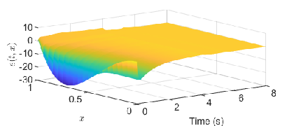
With , the feedback gain , and the observer gain , the sufficient conditions (34) of Theorem 11 are found feasible for when using an observer of dimension , ensuring the exponential stability of the closed-loop system in -norm. Simulation results are presented in Fig 2. It can be observed that the both state of the PDE and observation error converge exponentially to zero despite the strong impact of the sector nonlinearity applying on the control input as shown in Fig. 2(c). This is compliant with the theoretical predictions of Theorem 11. For the same system, the conditions of Corollary 14 that ensure the stability of the system in -norm appear to be more stringent from a numerical perspective. For instance, the sufficient conditions (34) and (35) of Corollary 14 are found feasible for when using an observer of dimension .
It can be observed in simulation that the reported control strategy cannot achieve the stabilization of the plant for arbitrarily large values of the size of the sector non linearity (23). Indeed, in the setting of the previous paragraph with a nonlinearity similar to the one of Fig 1 but rescaled with a size of the sector condition increased from to , we obtain in simulation divergent closed-loop system trajectories. Moreover, one can expect that the value of decreases with the level of instability of the open-loop plant (characterized by its growth bound), i.e, when decreasing the value of . This can be observed numerically by considering for example the constraints of Theorem 3 with and while placing the poles of both and at . In this case we obtain for a dimension of the observer: for , for , for , and for .


6 Conclusion
This paper has investigated the finite-dimensional observer-based stabilization of a reaction-diffusion equation in the presence of a sector nonlinearity in the control input. It is worth noting that even if the method has been presented in the case of a Robin boundary input with parameter and , the approach readily extends to the case and provided in (3) is selected sufficiently large positive so that (1) still holds and by replacing the change of variable (4) by for any fixed so that . Future research directions may be concern with extensions to other types of nonlinearities.
References
- [1] Mark J Balas. Finite-dimensional controllers for linear distributed parameter systems: exponential stability using residual mode filters. Journal of Mathematical Analysis and Applications, 133(2):283–296, 1988.
- [2] Dennis S Bernstein and Anthony N Michel. A chronological bibliography on saturating actuators. 5:375–380, 1995.
- [3] PJ Campo and M Morari. Robust control of processes subject to saturation nonlinearities. Computers & Chemical Engineering, 14(4-5):343–358, 1990.
- [4] Jean-Michel Coron and Emmanuel Trélat. Global steady-state controllability of one-dimensional semilinear heat equations. SIAM Journal on Control and Optimization, 43(2):549–569, 2004.
- [5] Jean-Michel Coron and Emmanuel Trélat. Global steady-state stabilization and controllability of 1D semilinear wave equations. Commun. Contemp. Math., 8(04):535–567, 2006.
- [6] Ruth Curtain. Finite-dimensional compensator design for parabolic distributed systems with point sensors and boundary input. IEEE Transactions on Automatic Control, 27(1):98–104, 1982.
- [7] Ruth F Curtain and Hans Zwart. An introduction to infinite-dimensional linear systems theory, volume 21. Springer Science & Business Media, 2012.
- [8] Stevan Dubljevic, Nael H El-Farra, Prashant Mhaskar, and Panagiotis D Christofides. Predictive control of parabolic PDEs with state and control constraints. International Journal of Robust and Nonlinear Control: IFAC-Affiliated Journal, 16(16):749–772, 2006.
- [9] Nael H El-Farra, Antonios Armaou, and Panagiotis D Christofides. Analysis and control of parabolic PDE systems with input constraints. Automatica, 39(4):715–725, 2003.
- [10] Lars Grüne and Thomas Meurer. Finite-dimensional output stabilization of linear diffusion-reaction systems–a small-gain approach. arXiv preprint arXiv:2104.06102, 2021.
- [11] Christian Harkort and Joachim Deutscher. Finite-dimensional observer-based control of linear distributed parameter systems using cascaded output observers. International Journal of Control, 84(1):107–122, 2011.
- [12] Rami Katz, Idan Basre, and Emilia Fridman. Delayed finite-dimensional observer-based control of 1D heat equation under neumann actuation. arXiv preprint arXiv:2011.10780, 2020.
- [13] Rami Katz and Emilia Fridman. Constructive method for finite-dimensional observer-based control of 1-D parabolic PDEs. Automatica, 122:109285, 2020.
- [14] Miroslav Krstic and Andrey Smyshlyaev. Boundary control of PDEs: A course on backstepping designs. SIAM, 2008.
- [15] Irena Lasiecka and Thomas I Seidman. Strong stability of elastic control systems with dissipative saturating feedback. Systems & Control Letters, 48(3-4):243–252, 2003.
- [16] Hugo Lhachemi and Christophe Prieur. Feedback stabilization of a class of diagonal infinite-dimensional systems with delay boundary control. IEEE Transactions on Automatic Control, 66(1):105–120, 2021.
- [17] Hugo Lhachemi and Christophe Prieur. Finite-dimensional observer-based boundary stabilization of reaction-diffusion equations with either a Dirichlet or Neumann boundary measurement. Automatica, 135:109955, 2022.
- [18] Hugo Lhachemi and Christophe Prieur. Finite-dimensional observer-based PI regulation control of a reaction-diffusion equation. IEEE Transactions on Automatic Control, page in press, 2022.
- [19] Hugo Lhachemi and Christophe Prieur. Local output feedback stabilization of a reaction-diffusion equation with saturated actuation. IEEE Transactions on Automatic Control, page in press, 2022.
- [20] Hugo Lhachemi, Christophe Prieur, and Robert Shorten. An LMI condition for the robustness of constant-delay linear predictor feedback with respect to uncertain time-varying input delays. Automatica, 109:108551, 2019.
- [21] Hugo Lhachemi, Christophe Prieur, and Emmanuel Trélat. PI regulation of a reaction-diffusion equation with delayed boundary control. IEEE Transactions on Automatic Control, 66(4):1573–1587, 2021.
- [22] Hugo Lhachemi and Robert Shorten. Boundary feedback stabilization of a reaction–diffusion equation with robin boundary conditions and state-delay. Automatica, 116:108931, 2020.
- [23] Weijiu Liu. Elementary feedback stabilization of the linear reaction-convection-diffusion equation and the wave equation, volume 66. Springer Science & Business Media, 2009.
- [24] Swann Marx, Vincent Andrieu, and Christophe Prieur. Cone-bounded feedback laws for -dissipative operators on Hilbert spaces. Mathematics of Control, Signals, and Systems, 29(4):1–32, 2017.
- [25] Swann Marx, Eduardo Cerpa, Christophe Prieur, and Vincent Andrieu. Global stabilization of a Korteweg–De Vries equation with saturating distributed control. SIAM Journal on Control and Optimization, 55(3):1452–1480, 2017.
- [26] Andrii Mironchenko, Christophe Prieur, and Fabian Wirth. Local stabilization of an unstable parabolic equation via saturated controls. IEEE Transactions on Automatic Control, 66(5):2162–2176, 2021.
- [27] Yury Orlov. On general properties of eigenvalues and eigenfunctions of a Sturm–Liouville operator: comments on ”ISS with respect to boundary disturbances for 1-D parabolic PDEs”. IEEE Transactions on Automatic Control, 62(11):5970–5973, 2017.
- [28] Yury Orlov, Yiming Lou, and Panagiotis D Christofides*. Robust stabilization of infinite-dimensional systems using sliding-mode output feedback control. International Journal of Control, 77(12):1115–1136, 2004.
- [29] Amnon Pazy. Semigroups of linear operators and applications to partial differential equations, volume 44. Springer Science & Business Media, 2012.
- [30] Christophe Prieur, Sophie Tarbouriech, and João Manoel Gomes da Silva Jr. Wave equation with cone-bounded control laws. IEEE Transactions on Automatic Control, 61(11):3452–3463, 2016.
- [31] Christophe Prieur and Emmanuel Trélat. Feedback stabilization of a 1D linear reaction-diffusion equation with delay boundary control. IEEE Transactions on Automatic Control, 64(4):1415–1425, 2019.
- [32] David L Russell. Controllability and stabilizability theory for linear partial differential equations: recent progress and open questions. SIAM Review, 20(4):639–739, 1978.
- [33] Yoshiyuki Sakawa. Feedback stabilization of linear diffusion systems. SIAM Journal on Control and Optimization, 21(5):667–676, 1983.
- [34] Marshall Slemrod. Feedback stabilization of a linear control system in Hilbert space with an a priori bounded control. Mathematics of Control, Signals and Systems, 2(3):265–285, 1989.
- [35] Sophie Tarbouriech, Germain Garcia, João Manoel Gomes da Silva Jr, and Isabelle Queinnec. Stability and stabilization of linear systems with saturating actuators. Springer Science & Business Media, 2011.
- [36] Sophie Tarbouriech, Isabelle Queinnec, Teodoro Alamo, Mirko Fiacchini, and Eduardo F Camacho. Ultimate bounded stability and stabilization of linear systems interconnected with generalized saturated functions. Automatica, 47(7):1473–1481, 2011.
- [37] Marius Tucsnak and George Weiss. Observation and control for operator semigroups. Springer Science & Business Media, 2009.
- [38] Luca Zaccarian and Andrew R Teel. Modern anti-windup synthesis: control augmentation for actuator saturation. Princeton University Press, 2011.
Appendix A Useful Lemma
Lemma 16.
Let , and Hurwitz, , , , , , and
We assume that there exist constants such that and for all and all . Moreover, we assume that there exists a constant such that , , and for all . Then there exists a constant such that, for any , there exists a symmetric matrix with such that and .